Olivecrona et al. J Cheminform (2017) 9:48 DOI 10.1186/s13321-017-0235-x

RESEARCH ARTICLE

Molecular de-novo design through deep reinforcement learningMarcus Olivecrona* , Thomas Blaschke, Ola Engkvist and Hongming Chen

Abstract

This work introduces a method to tune a sequence-based generative model for molecular de novo design that through augmented episodic likelihood can learn to generate structures with certain specified desirable properties. We demonstrate how this model can execute a range of tasks such as generating analogues to a query structure and generating compounds predicted to be active against a biological target. As a proof of principle, the model is first trained to generate molecules that do not contain sulphur. As a second example, the model is trained to generate analogues to the drug Celecoxib, a technique that could be used for scaffold hopping or library expansion start-ing from a single molecule. Finally, when tuning the model towards generating compounds predicted to be active against the dopamine receptor type 2, the model generates structures of which more than 95% are predicted to be active, including experimentally confirmed actives that have not been included in either the generative model nor the activity prediction model.

Keywords: De novo design, Recurrent neural networks, Reinforcement learning

© The Author(s) 2017. This article is distributed under the terms of the Creative Commons Attribution 4.0 International License (http://creativecommons.org/licenses/by/4.0/), which permits unrestricted use, distribution, and reproduction in any medium, provided you give appropriate credit to the original author(s) and the source, provide a link to the Creative Commons license, and indicate if changes were made. The Creative Commons Public Domain Dedication waiver (http://creativecommons.org/publicdomain/zero/1.0/) applies to the data made available in this article, unless otherwise stated.

BackgroundDrug discovery is often described using the metaphor of finding a needle in a haystack. In this case, the hay-stack comprises on the order of 1060−10100 syntheti-cally feasible molecules [1], out of which we need to find a compound which satisfies the plethora of criteria such as bioactivity, drug metabolism and pharmacokinetic (DMPK) profile, synthetic accessibility, etc. The fraction of this space that we can synthesize and test at all—let alone efficiently—is negligible. By using algorithms to vir-tually design and assess molecules, de novo design offers ways to reduce the chemical space into something more manageable for the search of the needle.

Early de novo design algorithms [1] used structure based approaches to grow ligands to sterically and elec-tronically fit the binding pocket of the target of interest [2, 3]. A limitation of these methods is that the molecules created often possess poor DMPK properties and can be synthetically intractable. In contrast, the ligand based

approach is to generate a large virtual library of chemi-cal structures, and search this chemical space using a scoring function that typically takes into account sev-eral properties such as DMPK profiles, synthetic acces-sibility, bioactivity, and query structure similarity [4, 5]. One way to create such a virtual library is to use known chemical reactions alongside a set of available chemical building blocks, resulting in a large number of syntheti-cally accessible structures [6]; another possibility is to use transformational rules based on the expertise of medici-nal chemists to design analogues to a query structure. For example, Besnard et al. [7] applied a transformation rule approach to the design of novel dopamine receptor type 2 (DRD2) receptor active compounds with specific poly-pharmacological profiles and appropriate DMPK profiles for a central nervous system indication. Although using either transformation or reaction rules can reliably and effectively generate novel structures, they are limited by the inherent rigidness and scope of the predefined rules and reactions.

A third approach, known as inverse Quantitative Struc-ture Activity Relationship (inverse QSAR), tackles the problem from a different angle: rather than first gener-ating a virtual library and then using a QSAR model to

Open Access

*Correspondence: m.olivecrona@gmail.com Hit Discovery, Discovery Sciences, Innovative Medicines and Early Development Biotech Unit, AstraZeneca R&D Gothenburg, 43183 Mölndal, Sweden

Page 2 of 14Olivecrona et al. J Cheminform (2017) 9:48

score and search this library, inverse QSAR aims to map a favourable region in terms of predicted activity to the corresponding molecular structures [8–10]. This is not a trivial problem: first the solutions of molecular descrip-tors corresponding to the region need to be resolved using the QSAR model, and these then need be mapped back to the corresponding molecular structures. The fact that the molecular descriptors chosen need to be suitable both for building a forward predictive QSAR model as well as for translation back to molecular structure is one of the major obstacles for this type of approach.

The Recurrent Neural Network (RNN) is commonly used as a generative model for data of sequential nature, and have been used successfully for tasks such as natu-ral language processing [11] and music generation [12]. Recently, there has been an increasing interest in using this type of generative model for the de novo design of molecules [13–15]. By using a data-driven method that attempts to learn the underlying probability distribution over a large set of chemical structures, the search over the chemical space can be reduced to only molecules seen as reasonable, without introducing the rigidity of rule based approaches. Segler et al. [13] demonstrated that an RNN trained on the canonicalized SMILES representation of molecules can learn both the syntax of the language as well as the distribution in chemical space. They also show how further training of the model using a focused set of actives towards a biological target can produce a fine-tuned model which generates a high fraction of predicted actives.

In two recent studies, reinforcement learning (RL) [16] was used to fine tune pre-trained RNNs. Yu et al. [15] use an adversarial network to estimate the expected return for state-action pairs sampled from the RNN, and by increasing the likelihood of highly rated pairs improves the generative network for tasks such as poem genera-tion. Jaques et al. [17] use Deep Q-learning to improve a pre-trained generative RNN by introducing two ways to score the sequences generated: one is a measure of how well the sequences adhere to music theory, and one is the likelihood of sequences according to the initial pre-trained RNN. Using this concept of prior likelihood they reduce the risk of forgetting what was initially learnt by the RNN, compared to a reward based only on the adher-ence to music theory. The authors demonstrate significant improvements over both the initial RNN as well as an RL only approach. They later extend this method to several other tasks including the generation of chemical struc-tures, and optimize toward molecular properties such as cLogP [18] and QED drug-likeness [19]. However, they report that the method is dependent on a reward function incorporating handwritten rules to penalize undesirable types of sequences, and even then can lead to exploitation of the reward resulting in unrealistically simple molecules

that are more likely to satisfy the optimization require-ments than more complex structures [17].

In this study we propose a policy based RL approach to tune RNNs for episodic tasks [16], in this case the task of generating molecules with given desirable prop-erties. Through learning an augmented episodic likeli-hood which is a composite of prior likelihood [17] and a user defined scoring function, the method aims to fine-tune an RNN pre-trained on the ChEMBL database [20] towards generating desirable compounds. Compared to maximum likelihood estimation finetuning [13], this method can make use of negative as well as continuous scores, and may reduce the risk of catastrophic forgetting [21]. The method is applied to several different tasks of molecular de novo design, and an investigation was car-ried out to illustrate how the method affects the behav-iour of the generative model on a mechanistic level.

MethodsRecurrent neural networksA recurrent neural network is an architecture of neural networks designed to make use of the symmetry across steps in sequential data while simultaneously at every step keeping track of the most salient information of pre-viously seen steps, which may affect the interpretation of the current one [22]. It does so by introducing the con-cept of a cell (Fig.  1). For any given step t, the cellt is a result of the previous cellt−1 and the current input xt−1 . The content of cellt will determine both the output at the current step as well as influence the next cell state. The cell thus enables the network to have a memory of past events, which can be used when deciding how to interpret new data. These properties make an RNN par-ticularly well suited for problems in the domain of natu-ral language processing. In this setting, a sequence of words can be encoded into one-hot vectors the length of our vocabulary X. Two additional tokens, GO and EOS, may be added to denote the beginning and end of the sequence respectively.

Learning the dataTraining an RNN for sequence modeling is typically done by maximum likelihood estimation of the next token xt

Cellt=1

P (x1)

GO

Cellt=2

P (x2)

x1

Cellt=3

P (x3)

x2

Cellt=4

P (EOS)

x3

Fig. 1 Learning the data. Depiction of maximum likelihood training of an RNN. xt are the target sequence tokens we are trying to learn by maximizing P(xt) for each step

Page 3 of 14Olivecrona et al. J Cheminform (2017) 9:48

in the target sequence given tokens for the previous steps (Fig. 1). At every step the model will produce a probabil-ity distribution over what the next character is likely to be, and the aim is to maximize the likelihood assigned to the correct token:

The cost function J (�), often applied to a subset of all training examples known as a batch, is minimized with respect to the network parameters �. Given a predicted log likelihood log P of the target at step t, the gradient of the prediction with respect to � is used to make an update of �. This method of fitting a neural network is called back-propagation. Due to the architecture of the RNN, changing the network parameters will not only affect the direct output at time t, but also affect the flow of information from the previous cell into the current one iteratively. This domino-like effect that the recur-rence has on back-propagation gives rise to some par-ticular problems, and back-propagation applied to RNNs is referred to as back-propagation through time (BPTT).

BPTT is dealing with gradients that through the chain-rule contains terms which are multiplied by themselves many times, and this can lead to a phenomenon known as exploding and vanishing gradients. If these terms are not unity, the gradients quickly become either very large or very small. In order to combat this issue, Hochreiter et al. introduced the Long-Short-Term Memory cell [23], which through a more controlled flow of information can decide what information to keep and what to discard. The Gated Recurrent Unit is a simplified implementation of the Long-Short-Term Memory architecture that achieves much of the same effect at a reduced computational cost [24].

Generating new samplesOnce an RNN has been trained on target sequences, it can then be used to generate new sequences that follow the conditional probability distributions learned from the training set. The first input—the GO token—is given and at every timestep after we sample an output token xt from the predicted probability distribution P(Xt) over our vocabulary X and use xt as our next input. Once the EOS token is sampled, the sequence is considered fin-ished (Fig. 2).

Tokenizing and one‑hot encoding SMILESA SMILES [25] represents a molecule as a sequence of characters corresponding to atoms as well as spe-cial characters denoting opening and closure of rings and branches. The SMILES is, in most cases, tokenized

J (�) = −

T∑

t=1

log P(xt | xt−1, . . . , x1)

based on a single character, except for atom types which comprise two characters such as “Cl” and “Br” and spe-cial environments denoted by square brackets (e.g [nH]), where they are considered as one token. This method of tokenization resulted in 86 tokens present in the train-ing data. Figure  3 exemplifies how a chemical structure is translated to both the SMILES and one-hot encoded representations.

There are many different ways to represent a single molecule using SMILES. Algorithms that always rep-resent a certain molecule with the same SMILES are referred to as canonicalization algorithms [26]. However, different implementations of the algorithms can still pro-duce different SMILES.

Reinforcement learningConsider an Agent, that given a certain state s ∈ S has to choose which action a ∈ A(s) to take, where S is the set of possible states and A(s) is the set of possible actions for that state. The policy π(a | s) of an Agent maps a state to the probability of each action taken therein.

Cellt=1

x1

GO

Cellt=2

x2

Cellt=3

x3

Cellt=4

EOS

Fig. 2 Generating sequences. Sequence generation by a trained RNN. Every timestep t we sample the next token of the sequence xt from the probability distribution given by the RNN, which is then fed in as the next input

Cl

N

NH

ClCc1c[nH]cn1

Cl C c 1 c nH c n 1

C 0 1 0 0 0 0 0 0 0

c 0 0 1 0 1 0 1 0 0

n 0 0 0 0 0 0 0 1 0

1 0 0 0 1 0 0 0 0 1

nH 0 0 0 0 0 1 0 0 0

Cl 1 0 0 0 0 0 0 0 0

Graph:

SMILES:

One-hotencoding:

Fig. 3 Three representations of 4-(chloromethyl)-1H-imidazole. Depiction of a one-hot representation derived from the SMILES of a molecule. Here a reduced vocabulary is shown, while in practice a much larger vocabulary that covers all tokens present in the training data is used

Page 4 of 14Olivecrona et al. J Cheminform (2017) 9:48

Many problems in reinforcement learning are framed as Markov decision processes, which means that the cur-rent state contains all information necessary to guide our choice of action, and that nothing more is gained by also knowing the history of past states. For most real prob-lems, this is an approximation rather than a truth; how-ever, we can generalize this concept to that of a partially observable Markov decision process, in which the Agent can interact with an incomplete representation of the environment. Let r(a | s) be the reward which acts as a measurement of how good it was to take an action at a certain state, and the long-term return G(at , St =

∑Tt rt)

as the cumulative rewards starting from t collected up to time T. Since molecular desirability in general is only sensible for a completed SMILES, we will refer only to the return of a complete sequence.

What reinforcement learning concerns, given a set of actions taken from some states and the rewards thus received, is how to improve the Agent policy in such a way as to increase the expected return E[G]. A task which has a clear endpoint at step T is referred to as an episodic task [16], where T corresponds to the length of the epi-sode. Generating a SMILES is an example of an episodic task, which ends once the EOS token is sampled.

The states and actions used to train the agent can be generated both by the agent itself or by some other means. If they are generated by the agent itself the learn-ing is referred to as on-policy, and if they are generated by some other means the learning is referred to as off-policy [16].

There are two different approaches often used in rein-forcement learning to obtain a policy: value based RL, and policy based RL [16]. In value based RL, the goal is to learn a value function that describes the expected return from a given state. Having learnt this function, a policy can be determined in such a way as to maximize the expected value of the state that a certain action will lead to. In policy based RL on the other hand, the goal is to directly learn a policy. For the problem addressed in this study, we believe that policy based methods is the natural choice for three reasons:

• Policy based methods can learn explicitly an optimal stochastic policy [16], which is our goal.

• The method used starts with a prior sequence model. The goal is to finetune this model according to some specified scoring function. Since the prior model already constitutes a policy, learning a finetuned policy might require only small changes to the prior model.

• The episodes in this case are short and fast to sample, reducing the impact of the variance in the estimate of the gradients.

In “Target activity guided structure generation“ section the change in policy between the prior and the finetuned model is investigated, providing justification for the sec-ond point.

The prior networkMaximum likelihood estimation was employed to train the initial RNN composed of 3 layers with 1024 Gated Recurrent Units (forget bias 5) in each layer. The RNN was trained on the RDKit [27] canoni-cal SMILES of 1.5 million structures from ChEMBL [20] where the molecules were restrained to contain-ing between 10 and 50 heavy atoms and elements ∈ {H ,B,C ,N ,O, F , Si,P, S,Cl,Br, I}. The model was trained with stochastic gradient descent for 50,000 steps using a batch size of 128, utilizing the Adam optimizer [28] (β1 = 0.9, β2 = 0.999, and ǫ = 10−8 ) with an initial learning rate of 0.001 and a 0.02 learning rate decay every 100 steps. Gradients were clipped to [−3, 3]. Tensorflow [29] was used to implement the Prior as well as the RL Agent.

The agent networkWe now frame the problem of generating a SMILES representation of a molecule with specified desirable properties via an RNN as a partially observable Markov decision process, where the agent must make a decision of what character to choose next given the current cell state. We use the probability distributions learnt by the previously described prior model as our initial prior pol-icy. We will refer to the network using the prior policy simply as the Prior, and the network whose policy has since been modified as the Agent. The Agent is thus also an RNN with the same architecture as the Prior. The task is episodic, starting with the first step of the RNN and ending when the EOS token is sampled. The sequence of actions A = a1, a2, . . . , aT during this epi-sode represents the SMILES generated and the product of the action probabilities P(A) =

∏Tt=1 π(at | st) repre-

sents the model likelihood of the sequence formed. Let S(A) ∈ [−1, 1] be a scoring function that rates the desir-ability of the sequences formed using some arbitrary method. The goal now is to update the agent policy π from the prior policy πPrior in such a way as to increase the expected score for the generated sequences. How-ever, we would like our new policy to be anchored to the prior policy, which has learnt both the syntax of SMILES and distribution of molecular structure in ChEMBL [13]. We therefore denote an augmented likelihood log P(A)U as a prior likelihood modulated by the desirability of a sequence:

log P(A)U = log P(A)Prior + σS(A)

Page 5 of 14Olivecrona et al. J Cheminform (2017) 9:48

where σ is a scalar coefficient. The return G(A) of a sequence A can in this case be seen as the agreement between the Agent likelihood log P(A)A and the aug-mented likelihood:

The goal of the Agent is to learn a policy which maxi-mizes the expected return, achieved by minimiz-ing the cost function J (�) = −G. The fact that we describe the target policy using the policy of the Prior and the scoring function enables us to formu-late this cost function. In the Additional file 1 we show how this approach can be described using a REIN-FORCE [30] algorithm with a final step reward of r(t) = [log P(A)U − log P(A)A]

2/ log P(A)A. We believe this is a more natural approach to the problem than REINFORCE algorithms directly using rewards of S(A) or log P(A)Prior + σS(A). In “Learning to avoid sulphur” section we compare our approach to these methods. The Agent is trained in an on-policy fashion on batches of 128 generated sequences, making an update to π after every batch has been generated and scored. A standard gradient descent optimizer with a learning rate of 0.0005 was used and gradients were clipped to [−3, 3].

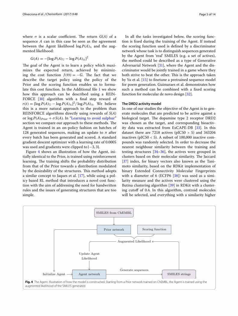
Figure  4 shows an illustration of how the Agent, ini-tially identical to the Prior, is trained using reinforcement learning. The training shifts the probability distribution from that of the Prior towards a distribution modulated by the desirability of the structures. This method adopts a similar concept to Jaques et al. [17], while using a pol-icy based RL method that introduces a novel cost func-tion with the aim of addressing the need for handwritten rules and the issues of generating structures that are too simple.

G(A) = −[log P(A)U − log P(A)A]2

In all the tasks investigated below, the scoring func-tion is fixed during the training of the Agent. If instead the scoring function used is defined by a discriminator network whose task is to distinguish sequences generated by the Agent from ‘real’ SMILES (e.g. a set of actives), the method could be described as a type of Generative Adversarial Network [31], where the Agent and the dis-criminator would be jointly trained in a game where they both strive to beat the other. This is the approach taken by Yu et al. [15] to finetune a pretrained sequence model for poem generation. Guimaraes et al. demonstrates how such a method can be combined with a fixed scoring function for molecular de novo design [32].

The DRD2 activity modelIn one of our studies the objective of the Agent is to gen-erate molecules that are predicted to be active against a biological target. The dopamine type 2 receptor DRD2 was chosen as the target, and corresponding bioactiv-ity data was extracted from ExCAPE-DB [33]. In this dataset there are 7218 actives (pIC50 > 5) and 343204 inactives (pIC50 < 5). A subset of 100,000 inactive com-pounds was randomly selected. In order to decrease the nearest neighbour similarity between the training and testing structures [34–36], the actives were grouped in clusters based on their molecular similarity. The Jaccard [37] index, for binary vectors also known as the Tani-moto similarity, based on the RDKit implementation of binary Extended Connectivity Molecular Fingerprints with a diameter of 6 (ECFP6 [38]) was used as a simi-larity measure and the actives were clustered using the Butina clustering algorithm [39] in RDKit with a cluster-ing cutoff of 0.4. In this algorithm, centroid molecules will be selected, and everything with a similarity higher

Agent network

Prior network

Initialize Agent

Scoring function

SMILES strings

SMILES from ChEMBL

Augmented Likelihood

Generate sequences

Update AgentLikelihood

Fig. 4 The Agent. Illustration of how the model is constructed. Starting from a Prior network trained on ChEMBL, the Agent is trained using the augmented likelihood of the SMILES generated

Page 6 of 14Olivecrona et al. J Cheminform (2017) 9:48

than 0.4 to these centroids will be assigned to the same cluster. The centroids are chosen such as to maximize the number of molecules that are assigned to any cluster. The clusters were sorted by size and iteratively assigned to the test, validation, and training sets (assigned 4 clusters each iteration) to give a distribution of 16,

16, and 46 of the clusters

respectively. The inactive compounds, of which less than 0.5% were found to belong to any of the clusters formed by the actives, were split randomly into the three sets using the same ratios.

A support vector machine (SVM) classifier with a Gaussian kernel was built in Scikit-learn [40] on the training set as a predictive model for DRD2 activity. The optimal C and Gamma values utilized in the final model were obtained from a grid search for the highest ROC-AUC performance on the validation set.

Results and discussionStructure generation by the PriorAfter the initial training, 94% of the sequences gener-ated by the Prior as described in “Generating new sam-ples” section corresponded to valid molecular structures according to RDKit [27] parsing, out of which 90% are novel structures outside of the training set. A set of ran-domly chosen structures generated by the Prior, as well as by Agents trained in the subsequent examples, are shown in the Additional file 2. The process of generating a SMILES by the Prior is illustrated in Fig.  5. For every token in the generated SMILES sequence, the conditional probability distribution over the vocabulary at this step according to the Prior is displayed. The sequence of dis-tributions are depicted in Fig. 5. For the first step, when no information other than the initial GO token is present, the distribution is an approximation of the distribution of first tokens for the SMILES in the ChEMBL training set. In this case “O” was sampled, but “C”, “N”, and the

halogens were all likely as well. Corresponding log likeli-hoods were −0.3 for “C”, −2.7 for “N”, −1.8 for “O”, and −5.0 for “F” and “Cl”.

A few (unsurprising) observations:

• Once the aromatic “n” has been sampled, the model has come to expect a ring opening (i.e. a number), since aromatic moieties by definition are cyclic.

• Once an aromatic ring has been opened, the aromatic atoms “c”, “n”, “o”, and “s” become probable, until 5 or 6 steps later when the model thinks it is time to close the ring.

• The model has learnt the RDKit canonicalized SMILES format of increasing ring numbers, and expects the first ring to be numbered “1”. Ring num-bers can be reused, as in the two first rings in this example. Only once “1” has been sampled does it expect a ring to be numbered “2” and so on.

Learning to avoid sulphurAs a proof of principle the Agent was first trained to gen-erate molecules which do not contain sulphur. The method described in “The Agent network” is compared with three other policy gradient based methods. The first alternative method is the same as the Agent method, with the only difference that the loss is defined on an action basis rather than on an episodic one, resulting in the cost function:

We refer to this method as ‘Action basis’. The second alter-native is a REINFORCE algorithm with a reward of S(A) given at the last step. This method is similar to the one used by Silver et al. to train the policy network in AlphaGo [41], as well as the method used by Yu et al. [15]. We refer

J(�) =

[

T∑

t=0

(log πPrior(at , st)− log π�(at , st))+ σS(A)

]2

O=C ( NC 1 CC 1 ) C 1 CCCN ( CC n 2 c c ( C ( F ) ( F ) F ) c c c 2 =O ) C 1 E

CcNnOoSsFCl()1234=E

Sampled SMILES

Cha

racters

−15

−10

−5

0

loge P StructureFig. 5 How the model thinks while generating the molecule on the right. Conditional probability over the next token as a function of previously chosen ones according to the model. On the y-axis is shown the probability distribution for the character to be choosen at the current step, and on the x-axis is shown the character that in this instance was sampled. E = EOS

Page 7 of 14Olivecrona et al. J Cheminform (2017) 9:48

to this method as ‘REINFORCE’. The corresponding cost function can be written as:

A variation of this method that considers prior likeli-hood is defined by changing the reward from S(A) to S(A)+ log P(A)Prior. This method is referred to as ‘REIN-FORCE + Prior’, with the cost function:

Note that the last method by nature strives to generate only the putative sequence with the highest reward. In contrast to the Agent, the optimal policy for this method is not stochastic. This tendency could be restrained by intro-ducing a regularizing policy entropy term. However, it was found that such regularization undermined the models ability to produce valid SMILES. This method is therefor dependent on only training sufficiently long for the model to reach a point where highly scored sequences are gener-ated, without being settled in a local minima. The experi-ment aims to answer the following questions:

• Can the models achieve the task of generating valid SMILES corresponding to structures that do not con-tain sulphur?

• Will the models exploit the reward function by converg-ing on naïve solutions such as ‘C’ if not imposed hand-written rules?

• Are the distributions of physical chemical properties for the generated structures similar to those of sulphur free structures generated by the Prior?

The task is defined by the following scoring function:

J (�) = S(A)

T∑

t=0

log π�(at , st)

J (�) = [log P(A)Prior + σS(A)]

T∑

t=0

log π�(at , st)

S(A) =

1 if valid and no S0 if not valid−1 if contains S

All the models were trained for 1000 steps starting from the Prior and 12,800 SMILES sequences were sampled from all the models as well as the Prior. A learning rate of 0.0005 was used for the Agent and Action basis methods, and 0.0001 for the two REINFORCE methods. The val-ues of σ used were 2 for the Agent and ‘REINFORCE + Prior’, and 8 for ‘Action basis’. To explore what effect the training has on the structures generated, relevant prop-erties for non sulphur containing structures generated by both the Prior and the other models were compared. The molecular weight, cLogP, the number of rotatable bonds, and the number of aromatic rings were all calcu-lated using RDKit. The experiment was repeated three times with different random seeds. The results are shown in Table 1 and randomly selected SMILES generated by the Prior and the different models can be seen in Table 2. For the ‘REINFORCE’ method, where the sole aim is to generate valid SMILES that do not contain sulphur, the model quickly learns to exploit the reward funtion by generating sequences containing predominately ‘C’. This is not surprising, since any sequence consisting only of this token always gets rewarded. For the ‘REINFORCE + Prior’ method, the inclusion of the prior likelihood in the reward function means that this is no longer a viable strategy (the sequences would be given a low prior prob-ability). The model instead tries to find the structure with the best combination of score and prior likelihood, but as is evident from the SMILES generated and the statistics shown in Table  1, this results in small, simplistic struc-tures being generated. Thus, both REINFORCE algo-rithms managed to achieve high scores according to the scoring function, but poorly represented the Prior. Both the Agent and the ‘Action basis’ methods have explicitly specified target policies. For the ‘Action basis’ method the policy is specified exactly on a stepwise level, while for the Agent the target policy is only specified to the like-lihoods of entire sequences. Although the ‘Action basis’ method generates structures that are more similar to the Prior than the two REINFORCE methods, it performed worse than the Agent despite the higher value of σ used while also being slower to learn. This may be due to the

Table 1 Comparison of model performance and properties for non-sulphur containing structures generated by the two models

Properties reported as Mean ± SD

Model Prior Agent Action basis REINFORCE REINFORCE + Prior

Fraction of valid SMILES 0.94 ± 0.01 0.95 ± 0.01 0.95 ± 0.01 0.98 ± 0.00 0.98 ± 0.00

Fraction without sulphur 0.66 ± 0.01 0.98 ± 0.00 0.92 ± 0.02 0.98 ± 0.00 0.92 ± 0.01

Average molecular weight 371 ± 1.70 367 ± 3.30 372 ± 0.94 585 ± 27.4 232 ± 5.25

Average cLogP 3.36 ± 0.04 3.37 ± 0.09 3.39 ± 0.02 11.3 ± 0.85 3.05 ± 0.02

Average NumRotBonds 5.39 ± 0.04 5.41 ± 0.07 6.08 ± 0.04 30.0 ± 2.17 2.8 ± 0.11

Average NumAromRings 2.26 ± 0.02 2.26 ± 0.02 2.09 ± 0.02 0.57 ± 0.04 2.11 ± 0.02

Page 8 of 14Olivecrona et al. J Cheminform (2017) 9:48

less restricted target policy of the Agent, which could facilitate optimization. The Agent achieved the same fraction of sulphur free structures as the REINFORCE algorithms, while seemingly doing a much better job of representing the Prior. This is indicated by the similar-ity of the properties of the generated structures shown in Table  1 as well as the SMILES themselves shown in Table 2.

Similarity guided structure generationThe second task investigated was that of generating structures similar to a query structure. The Jaccard index [37] Ji,j of the RDKit implementation of FCFP4 [38] fin-gerprints was used as a similarity measure between mol-ecules i and j. Compared to the DRD2 activity model (“The DRD2 activity model” section), the feature invari-ant version of the fingerprints and the smaller diameter 4 was used in order to get a more fuzzy similarity measure. The scoring function was defined as:

This definition means that an increase in similarity is only rewarded up to the point of k ∈ [0, 1], as well as scal-ing the reward from −1 (no overlap in the fingerprints between query and generated structure) to 1 (at least k degree of overlap). Celecoxib was chosen as our query structure, and we first investigated whether Celecoxib itself could be generated by using the high values of k = 1 and σ = 15. The Agent was trained for 1000 steps. After a 100 training steps the Agent starts to generate Celecoxib, and after 200 steps it predominately generates this struc-ture (Fig. 6).

S(A) = −1+ 2×min{Ji,j , k}

k

Celecoxib itself as well as many other similar struc-tures appear in the ChEMBL training set used to build the Prior. An interesting question is whether the Agent could succeed in generating Celecoxib when these struc-tures are not part of the chemical space covered by the Prior. To investigate this, all structures with a similar-ity to Celecoxib higher than 0.5 (corresponding to 1804 molecules) were removed from the training set and a new reduced Prior was trained. The prior likelihood of Celecoxib for the canonical and reduced Priors was

Table 2 Randomly selected SMILES generated by the different models

Model Sampled SMILES

Prior CCOC(=O)C1=C(C)OC(N)=C(C#N)C1c1ccccc1C(F)(F)F

COC(=O)CC(C)=NNc1ccc(N(C)C)cc1[N+](=O)[O-]

Cc1ccccc1CNS(=O)(=O)c1ccc2c(c1)C(=O)C(=O)N2

Agent CC(C)(C)NC(=O)c1ccc(OCc2ccccc2C(F)(F)F)nc1-c1ccccc1

CC(=O)NCC1OC(=O)N2c3ccc(-c4cccnc4)cc3OCC12

OCCCNCc1cccc(-c2cccc(-c3nc4ccccc4[nH]3)c2OCCOc2ncc(Cl)cc2Br)c1

Action level CCN1CC(C)(C)OC(=O)c2cc(-c3ccc(Cl)cc3)ccc21

CCC(CC)C(=O)Nc1ccc2cnn(-c3ccc(C(C)=O)cc3)c2c1

CCCCN1C(=O)c2ccccc2NC1c1ccc(OC)cc1

REINFORCE CC1CCCCC12NC(=O)N(CC(=O)Nc1ccccc1C(=O)O)C2=O

CCCCCCCCCCCCCCCCCCCCCCCCCCCCNC(=O)OCCCCCC

CCCCCCCCCCCCCCCCCCCCCC1CCC(O)C1(CCC)CCCCCCCCCCCCCCC

REINFORCE + Prior Nc1ccccc1C(=O)Oc1ccccc1

O=c1cccccc1Oc1ccccc1

Nc1ccc(-c2ccccc2O)cc1

0 200 400 600 800 1,0000.25

0.7

1

Training steps

Average

J

Canonical prior k = 1 σ = 15Canonical prior k = 0.7 σ = 12Reduced prior k = 1 σ = 15Reduced prior k = 0.7 σ = 12Reduced prior k = 0.7 σ = 15

Fig. 6 Average similarity J of generated structures as a function of training steps. Difference in learning dynamics for the Agents based on the canonical Prior, and those based on a reduced Prior where everything more similar than J = 0.5 to Celecoxib have been removed

Page 9 of 14Olivecrona et al. J Cheminform (2017) 9:48

compared, as well as the ability of the models to gener-ate structures similar to Celecoxib. As expected, the prior probability of Celecoxib decreased when similar compounds were removed from the training set from loge P = −12.7 to loge P = −19.2, representing a reduc-tion in likelihood of a factor of 700. An Agent was then trained using the same hyperparameters as before, but on the reduced Prior. After 400 steps, the Agent again man-aged to find Celecoxib, albeit requiring more time to do so. After 1000 steps, Celecoxib was the most commonly generated structure (about a third of the generated struc-tures), followed by demethylated Celecoxib (also a third) whose SMILES is more likely according to the Prior with loge P = −15.2 but has a lower similarity (J = 0.87 ), resulting in an augmented likelihood equal to that of Celecoxib.

These experiments demonstrate that the Agent can be optimized using fingerprint based Jaccard similarity as the objective, but making copies of the query structure is hardly useful. A more useful example is that of generating structures that are moderately to the query structure. The Agent was therefore trained for 3000 steps, starting from both the canonical as well as the reduced Prior, using k = 0.7 and σ = 12. The Agents based on the canonical Prior quickly converge to their targets, while the Agents based on the reduced Prior converged more slowly. For the Agent based on the reduced Prior where k = 1, the fact that Celecoxib and demethylated Celecoxib are given similar augmented likelihoods means that the average similarity converges to around 0.9 rather than 1.0. For the Agent based on the reduced Prior where k = 0.7, the lower prior likelihood of compounds similar to Celecoxib translates to a lower augmented likelihood, which lowers the average similarity of the structures generated by the Agent.

To explore whether this reduced prior likelihood could be offset with a higher value of σ, an Agent starting from the reduced Prior was trained using σ = 15. Though tak-ing slightly more time to converge than the Agent based on the canonical Prior, this Agent too could converge to the target similarity. The learning curves for the different model is shown in Fig. 6.

An illustration of how the type of structures generated by the Agent evolves during training is shown in Fig. 7. For the Agent based on the reduced Prior with k = 0.7 and σ = 15, three structures were randomly sampled every 100 training steps from step 0 up to step 400. At first, the structures are not similar to Celecoxib. After 200 steps, some features from Celecoxib have started to emerge, and after 300 steps the model generates mostly close analogues of Celecoxib.

We have investigated how various factors affect the learning behaviour of the Agent. In real drug discovery

applications, we might be more interested in finding structures with modest similarity to our query mol-ecules rather than very close analogues. For example, one of the structures sampled after 200 steps shown in Fig.  7 displays a type of scaffold hopping where the sulphur functional group on one of the outer aromatic rings has been fused to the central pyrazole. The simi-larity to Celecoxib of this structure is 0.4, which may be a more interesting solution for scaffold-hopping pur-poses. One can choose hyperparameters and similarity criterion tailored to the desired output. Other types of similarity measures such as pharmacophoric finger-prints [42], Tversky substructure similarity [43], or presence/absence of certain pharmacophores could also be explored.

Target activity guided structure generationThe third example, perhaps the one most interesting and relevant for drug discovery, is to optimize the Agent towards generating structures with predicted biologi-cal activity. This can be seen as a form of inverse QSAR, where the Agent is used to implicitly map high predicted probability of activity to molecular structure. DRD2 was chosen as the biological target. The clustering split of the DRD2 activity dataset as described in “The DRD2 activity model” section resulted in 1405, 1287, and 4526 actives in the test, validation, and training sets respectively. The average similarity to the nearest neighbour in the train-ing set for the test set compounds was 0.53. For a random split of actives in sets of the same sizes this similarity was 0.69, indicating that the clustering had significantly decreased training-test set similarity which mimics the hit finding practice in drug discovery to identify diverse hits to the training set. Most of the DRD2 actives are also included in the ChEMBL dataset used to train the Prior. To explore the effect of not having the known actives included in the Prior, a reduced Prior was trained on a reduced subset of the ChEMBL training set where all DRD2 actives had been removed.

The optimal hyperparameters found for the SVM activ-ity model were C = 27, γ = 2−6, resulting in a model whose performance is shown in Table  3. The good per-formance in general can be explained by the apparent dif-ference between actives and inactive compounds as seen during the clustering, and the better performance on the test set compared to the validation set could be due to slightly higher nearest neighbour similarity to the train-ing actives (0.53 for test actives and 0.48 for validation actives).

The output of the DRD2 model for a given structure is an uncalibrated predicted probability of being active Pactive. This value is used to formulate the following scor-ing function:

Page 10 of 14Olivecrona et al. J Cheminform (2017) 9:48

The model was trained for 3000 steps using σ = 7. After training, the fraction of predicted actives according to the DRD2 model increased from 0.02 for structures

S(A) = −1+ 2× Pactivegenerated by the reduced Prior to 0.96 for structures gen-erated by the corresponding Agent network (Table 4). To see how well the structure-activity-relationship learnt by the activity model is transferred to the type of structures generated by the Agent RNN, the fraction of compounds with an ECFP6 Jaccard similarity greater than 0.4 to any active in the training and test sets was calculated.

In some cases, the model recovered exact matches from the training and test sets (c.f. Segler et al. [13]). The fraction of recovered test actives recovered by the canon-ical and reduced Prior were 1.3 and 0.3% respectively. The Agent derived from the canonical Prior managed to recover 13% test actives; the Agent derived from the reduced Prior recovered 7%. For the Agent derived from the reduced Prior, where the DRD2 actives were excluded

0 100 200 300 400

Training steps

Celecoxib

Fig. 7 Evolution of generated structures during training Structures sampled every 100 training steps during the training of the Agent towards similarity to Celecoxib with k = 0.7 and σ = 15

Table 3 Performance of the DRD2 activity model

Set Training Validation Test

Accuracy 1.00 0.98 0.98

ROC-AUC 1.00 0.99 1.00

Precision 1.00 0.96 0.97

Recall 1.00 0.73 0.82

Page 11 of 14Olivecrona et al. J Cheminform (2017) 9:48

from the Prior training set, this means that the model has learnt to generate “novel” structures that have been seen neither by the DRD2 activity model nor the Prior, and are experimentally confirmed actives. We can formalize this observation by calculating the probability of a given gen-erated sequence belonging to the set of test actives. For the canonical and reduced Priors, this probability was 0.17× 10−3 and 0.05× 10−3 respectively. Removing the actives from the Prior thus resulted in a threefold reduc-tion in the probability of generating a structure from the set of test actives. For the Agents, the probabilities rose to 15.0× 10−3 and 40.2× 10−3 respectively, corresponding to an enrichment of a factor of 250 over the Prior mod-els. Again the consequence of removing the actives from the Prior was a threefold reduction in the probability of

generating a test set active: the difference between the two Priors is directly mirrored by their corresponding Agents. Apart from generating a higher fraction of struc-tures that are predicted to be active, both Agents also generate a significantly higher fraction of valid SMILES (Table 4). Sequences that are not valid SMILES receive a score of −1, which means that the scoring function natu-rally encourages valid SMILES.

A few of the test set actives generated by the Agent based on the reduced Prior along with a few randomly selected generated structures are shown together with their predicted probability of activity in Fig. 8. Encourag-ingly, the recovered test set actives vary considerably in their structure, which would not have been the case had the Agent converged to generating only a certain type of very similar predicted active compounds.

Removing the known actives from the training set of the Prior resulted in an Agent which shows a decrease in all metrics measuring the overlap between the known actives and the structures generated, compared to the Agent derived from the canonical Prior. Interestingly, the fraction of predicted actives did not change significantly. This indicates that the Agent derived from the reduced Prior has managed to find a similar chemical space to that of the canonical Agent, with structures that are equally likely to be predicted as active, but are less similar to the known actives. Whether or not these compounds are active will be dependent on the accuracy of the target activity model. Ideally, any predictive model to be used in conjunction with the generative model should cover a

Table 4 Comparison of  properties for  structures gener-ated by  the canonical Prior, the reduced Prior, and  corre-sponding Agents

a DRD2 actives witheld from the training of the Prior

Model Prior Agent Priora Agenta

Fraction valid SMILES 0.94 0.99 0.94 0.99

Fraction predicted actives 0.03 0.97 0.02 0.96

Fraction similar to train active 0.02 0.79 0.02 0.75

Fraction similar to test active 0.01 0.46 0.01 0.38

Fraction of test actives recovered (×10

−3)13.5 126 2.85 72.6

Probability of generating a test set active (×10

−3)0.17 40.2 0.05 15.0

Recovered test actives

Pactive 0.95 0.95 0.73 0.66

Randomly selected

Pactive 1.00 0.99 0.98 1.00

Fig. 8 Structures designed by the Agent to target DRD2. Molecules generated by the Agent based on the reduced Prior. On the top are four of the test set actives that were recovered, and below are four randomly selected structures. The structures are annotated with the predicted probability of being active

Page 12 of 14Olivecrona et al. J Cheminform (2017) 9:48

broad chemical space within its domain of applicability, since it initially has to assess representative structures of the dataset used to build the Prior [13].

Figure 9 shows a comparison of the conditional prob-ability distributions for the reduced Prior and its cor-responding Agent when a molecule from the set of test actives is generated. It can be seen that the changes are not drastic with most of the trends learnt by the Prior being carried over to the Agent. However, a big change in the probability distribution even only at one step can have a large impact on the likelihood of the sequence and could significantly alter the type of structures generated.

ConclusionTo summarize, we believe that an RNN operating on the SMILES representation of molecules is a promising method for molecular de novo design. It is a data-driven generative model that does not rely on pre-defined build-ing blocks and rules, which makes it clearly differentiated from traditional methods. In this study we extend upon previous work [13–15, 17] by introducing a reinforce-ment learning method which can be used to tune the RNN to generate structures with certain desirable prop-erties through augmented episodic likelihood.

The model was tested on the task of generating sulphur free molecules as a proof of principle, and the method using augmented episodic likelihood was compared with traditional policy gradient methods. The results indicate that the Agent can find solutions reflecting the underly-ing probability distribution of the Prior, representing a significant improvement over both traditional REIN-FORCE [30] algorithms as well as previously reported methods [17]. To evaluate if the model could be used to generate analogues to a query structure, the Agent was trained to generate structures similar to the drug Celecoxib. Even when all analogues of Celecoxib were removed from the Prior, the Agent could still locate the

intended region of chemical space which was not part of the Prior. Further more, when trained towards generat-ing predicted actives against the dopamine receptor type 2 (DRD2), the Agent generates structures of which more than 95% are predicted to be active, and could recover test set actives even in the case where they were not included in either the activity model nor the Prior. Our results indicate that the method could be a useful tool for drug discovery.

It is clear that the qualities of the Prior are reflected in the corresponding Agents it produces. An exhaustive study which explores how parameters such as training set size, model size, regularization [44, 45], and training time would influence the quality and variety of structures gen-erated by the Prior would be interesting. Another inter-esting avenue for future research might be that of token embeddings [46]. The method was found to be robust with respect to the hyperparameters σ and the learning rate.

All of the aforementioned examples used single param-eter based scoring functions. In a typical drug discov-ery project, multiple parameters such as target activity, DMPK profile, synthetic accessibility etc. all need to be taken into account simultaneously. Applying this type of multi-parametric scoring functions to the model is an area requiring further research.

AbbreviationsDMPK: drug metabolism and pharmacokinetics; DRD2: dopamine receptor D2; QSAR: quantitive structure activity relationship; RNN: recurrent neural network;

Additional files

Additional file 1. Equivalence to REINFORCE. Proof that the method used can be described as a REINFORCE type algorithm.

Additional file 2. Generated structures. Structures generated by the canonical Prior and different Agents.

COc 1 c c c c c 1N1CCN (CCCCNC (=O) c 2 c c c c c 2 I ) CC1E

CcNnOoSsFCl()1234=E

Sampled SMILES

Cha

racters

Prior

COc 1 c c c c c 1N1CCN (CCCCNC (=O) c 2 c c c c c 2 I ) CC1E

Sampled SMILES

Agent

−15

−10

−5

0

loge PFig. 9 A (small) change of mind. The conditional probability distributions when the DRD2 test set active ‘COc1ccccc1N1CCN(CCCCNC(=O)c2ccccc2I)CC1’ is generated by the Prior and an Agent trained using the DRD2 activity model, for the case where all actives used to build the activity model have been removed from the Prior. E = EOS

Page 13 of 14Olivecrona et al. J Cheminform (2017) 9:48

RL: reinforcement Learning; Log: natural logarithm; BPTT: back-propagation through time; A: sequence of tokens constituting a SMILES; Prior: an RNN trained on SMILES from ChEMBL used as a starting point for the Agent; Agent: an RNN derived from a Prior, trained using reinforcement learning; J: Jaccard index; ECFP6: Extended Molecular Fingerprints with diameter 6; SVM: support vector machine; FCFP4: Extended Molecular Fingerprints with diameter 4 and feature invariants.

Authors’ contributionsMO contributed concept and implementation. All authors co-designed experiments. All authors contributed to the interpretation of results. MO wrote the manuscript. HC, TB, and OE reviewed and edited the manuscript. All authors read and approved the final manuscript.

AcknowledgementsThe authors thank Thierry Kogej and Christian Tyrchan for general assistance and discussion, and Dominik Peters for his expertise in LATEX.

Competing interestsThe authors declare that they have no competing interests.

Availability of data and materialsThe source code and data supporting the conclusions of this article is available at https://github.com/MarcusOlivecrona/REINVENT, doi:10.5281/zenodo.572576.Project name: REINVENTProject home page: https://github.com/MarcusOlivecrona/REINVENTArchived version: http://doi.org/10.5281/zenodo.572576Operating system: Platform independentProgramming language: PythonOther requirements: Python2.7, Tensorflow, RDKit, Scikit-learnLicense: MIT.

Consent for publicationNot applicable.

Ethics approval and consent to participateNot applicable.

FundingMO, HC, and OE are employed by AstraZeneca. TB has received funding from the European Union’s Horizon 2020 research and innovation program under the Marie Sklodowska-Curie grant agreement No 676434, “Big Data in Chemistry” (“BIGCHEM”, http://bigchem.eu). The article reflects only the authors’ view and neither the European Commission nor the Research Executive Agency (REA) are responsible for any use that may be made of the information it contains.

Publisher’s NoteSpringer Nature remains neutral with regard to jurisdictional claims in pub-lished maps and institutional affiliations.

Received: 14 May 2017 Accepted: 23 August 2017

References 1. Schneider G, Fechner U (2005) Computer-based de novo design of drug-

like molecules. Nat Rev Drug Discov 4(8):649–663. doi:10.1038/nrd1799 2. Böhm HJ (1992) The computer program ludi: a new method for the de

novo design of enzyme inhibitors. J Comput Aided Mol Des 6(1):61–78. doi:10.1007/BF00124387

3. Gillet VJ, Newell W, Mata P, Myatt G, Sike S, Zsoldos Z, Johnson AP (1994) Sprout: recent developments in the de novo design of molecules. J Chem Inf Comput Sci 34(1):207–217. doi:10.1021/ci00017a027

4. Ruddigkeit L, Blum LC, Reymond JL (2013) Visualization and virtual screening of the chemical universe database gdb-17. J Chem Inf Model 53(1):56–65. doi:10.1021/ci300535x

5. Hartenfeller M, Zettl H, Walter M, Rupp M, Reisen F, Proschak E, Weggen S, Stark H, Schneider G (2012) Dogs: reaction-driven de novo design of bioactive compounds. PLOS Comput Biol 8:1–12. doi:10.1371/journal.pcbi.1002380

6. Schneider G, Geppert T, Hartenfeller M, Reisen F, Klenner A, Reutlinger M, Hähnke V, Hiss JA, Zettl H, Keppner S, Spänkuch B, Schneider P (2011) Reaction-driven de novo design, synthesis and testing of potential type II kinase inhibitors. Future Med Chem 3(4):415–424. doi:10.4155/fmc.11.8

7. Besnard J, Ruda GF, Setola V, Abecassis K, Rodriguiz RM, Huang X-P, Norval S, Sassano MF, Shin AI, Webster LA, Simeons FRC, Stojanovski L, Prat A, Seidah NG, Constam DB, Bickerton GR, Read KD, Wetsel WC, Gilbert IH, Roth BL, Hopkins AL (2012) Automated design of ligands to polypharma-cological profiles. Nature 492(7428):215–220. doi:10.1038/nature11691

8. Miyao T, Kaneko H, Funatsu K (2016) Inverse qspr/qsar analysis for chemi-cal structure generation (from y to x). J Chem Inf Model 56(2):286–299. doi:10.1021/acs.jcim.5b00628

9. Churchwell CJ, Rintoul MD, Martin S Jr, Visco DP, Kotu A, Larson RS, Sillerud LO, Brown DC, Faulon J-L (2004) The signature molecular descriptor: 3. Inverse-quantitative structure-activity relationship of icam-1 inhibitory pep-tides. J Mol Graph Model 22(4):263–273. doi:10.1016/j.jmgm.2003.10.002

10. Wong WW, Burkowski FJ (2009) A constructive approach for discovering new drug leads: using a kernel methodology for the inverse-qsar prob-lem. J Cheminform 1:44. doi:10.1186/1758-2946-1-4

11. Mikolov T, Karafiát M, Burget L, Cernock‘y J, Khudanpur S (2010) Recur-rent neural network based language model. In: Kobayashi T, Hirose K, Nakamura S (eds) 11th annual conference of the international speech communication association (INTERSPEECH 2010), Makuhari, Chiba, Japan. ISCA, 26–30 Sept 2010

12. Eck D, Schmidhuber J (2002) A first look at music composition using lstm recurrent neural networks. Technical report, Istituto Dalle Molle Di Studi Sull Intelligenza Artificiale

13. Segler MHS, Kogej T, Tyrchan C, Waller MP (2017) Generating focussed molecule libraries for drug discovery with recurrent neural networks. arXiv:1701.01329

14. Gómez-Bombarelli R, Duvenaud DK, Hernáandez-Lobato JM, Aguilera-Iparraguirre J, Hirzel TD, Adams RP, Aspuru-Guzik A (2016) Automatic chemical design using a data-driven continuous representation of molecules. CoRR. arXiv:1610.02415

15. Yu L, Zhang W, Wang J, Yu Y (2016) Seqgan: sequence generative adver-sarial nets with policy gradient. CoRR. arXiv:1609.05473

16. Sutton R, Barton A (1998) Reinforcement learning: an introduction, 1st edn. MIT Press, Cambridge

17. Jaques N, Gu S, Turner RE, Eck D (2016) Tuning recurrent neural networks with reinforcement learning. CoRR. arXiv:1611.02796

18. Leo A, Hansch C, Elkins D (1971) Partition coefficients and their uses. Chem Rev 71(6):525–616. doi:10.1021/cr60274a001

19. Bickerton GR, Paolini GV, Besnard J, Muresan S, Hopkins AL (2012) Quantifying the chemical beauty of drugs. Nat Chem 4:90–98. doi:10.1038/nchem.1243

20. Gaulton A, Bellis LJ, Bento AP, Chambers J, Davies M, Hersey A, Light Y, McGlinchey S, Michalovich D, Al-Lazikani B, Overington JP (2012) Chembl: a large-scale bioactivity database for drug discovery. Nucleic Acids Res 40:1100–1107. doi:10.1093/nar/gkr777 Version 22

21. Goodfellow IJ, Mirza M, Xiao D, Courville A, Bengio Y (2013) An empirical investigation of catastrophic forgetting in gradient-based neural net-works. arXiv:1312.6211

22. Goodfellow I, Bengio Y, Courville A (2016) Deep learning, 1st edn. MIT Press, Cambridge

23. Hochreiter S, Schmidhuber J (1997) Long short-term memory. Neural Comput 9(8):1735–1780. doi:10.1162/neco.1997.9.8.1735

24. Chung J, Gulcehre C, Cho K, Bengio Y (2014) Empirical evaluation of gated recurrent neural networks on sequence modeling. arXiv:1412.3555

25. SMILES. http://www.daylight.com/dayhtml/doc/theory/theory.smiles.html. Accessed 7 Apr 2017

26. Weininger D, Weininger A, Weininger JL (1989) Smiles. 2. Algorithm for generation of unique smiles notation. J Chem Inf Comput Sci 29(2):97–101. doi:10.1021/ci00062a008

27. RDKit: open source cheminformatics. Version: 2016-09-3. http://www.rdkit.org/

28. Kingma DP, Ba J: Adam (2014) A method for stochastic optimization. CoRR. arXiv:1412.6980

29. Tensorflow. Version: 1.0.1. http://www.tensorflow.org

Page 14 of 14Olivecrona et al. J Cheminform (2017) 9:48

30. Williams RJ (1992) Simple statistical gradient-following algorithms for connectionist reinforcement learning. Mach Learn 8(3):229–256

31. Goodfellow I, Pouget-Abadie J, Mirza M, Xu B, Warde-Farley D, Ozair S, Courville A, Bengio Y (2014) Generative adversarial nets. In: Ghahramani Z, Welling M, Cortes C, Lawrence ND, Weinberger KQ (eds) Advances in neural information processing systems 27 (NIPS 2014), Montreal, Quebec, Canada. NIPS foundation, 8–13 Dec 2014

32. Lima Guimaraes G, Sanchez-Lengeling B, Cunha Farias PL, Aspuru-Guzik A (2017) Objective-reinforced generative adversarial networks (ORGAN) for sequence generation models. arXiv:1705.10843

33. Sun J, Jeliazkova N, Chupakin V, Golib-Dzib J-F, Engkvist O, Carlsson L, Wegner J, Ceulemans H, Georgiev I, Jeliazkov V, Kochev N, Ashby TJ, Chen H (2017) Excape-db: an integrated large scale dataset facilitating big data analysis in chemogenomics. J Cheminform 9(1):17. doi:10.1186/s13321-017-0203-5

34. Sheridan RP (2013) Time-split cross-validation as a method for estimating the goodness of prospective prediction. J Chem Inf Model 53(4):783–790

35. Unterthiner T, Mayr A, Steijaert M, Wegner JK, Ceulemans H, Hochreiter S (2014) Deep learning as an opportunity in virtual screening. In: Deep learning and representation learning workshop. NIPS, pp 1058–1066

36. Mayr A, Klambauer G, Unterthiner T, Hochreiter S (2016) Deeptox: toxicity prediction using deep learning. Front Environ Sci 3:80

37. Jaccard P (1901) Étude comparative de la distribution florale dans une portion des Alpes et des Jura. Bull Soc Vaud Sci Nat 37:547–579

38. Rogers D, Hahn M (2010) Extended-connectivity fingerprints. J Chem Inf Model 50(5):742–754. doi:10.1021/ci100050t

39. Butina D (1999) Unsupervised data base clustering based on daylight’s fingerprint and tanimoto similarity: a fast and automated way to

cluster small and large data sets. J Chem Inf Comput Sci 39(4):747–750. doi:10.1021/ci9803381

40. Pedregosa F, Varoquaux G, Gramfort A, Michel V, Thirion B, Grisel O, Blondel M, Prettenhofer P, Weiss R, Dubourg V, Vanderplas J, Passos A, Cournapeau D, Brucher M, Perrot M, Duchesnay E (2011) Scikit-learn: machine learning in Python. J Mach Learn Res 12:2825–2830 Version 0.17

41. Silver D, Huang A, Maddison CJ, Guez A, Sifre L, Van Den Driessche G, Schrittwieser J, Antonoglou I, Panneershelvam V, Lanctot M et al (2016) Mastering the game of go with deep neural networks and tree search. Nature 529(7587):484–489

42. Reutlinger M, Koch CP, Reker D, Todoroff N, Schneider P, Rodrigues T, Sch-neider G (2013) Chemically advanced template search (CATS) for scaffold-hopping and prospective target prediction for ’orphan’ molecules. Mol Inform 32(2):133–138

43. Senger S (2009) Using Tversky similarity searches for core hopping: find-ing the needles in the haystack. J Chem Inf Model 49(6):1514–1524

44. Zaremba W, Sutskever I, Vinyals O (2014) Recurrent neural network regu-larization. CoRR. arXiv:1409.2329

45. Wan L, Zeiler M, Zhang S, LeCun Y, Fergus R (2013) Regularization of neu-ral networks using dropconnect. In: Proceedings of the 30th international conference on international conference on machine learning, Vol 28. ICML’13, pp 1058–1066

46. Bengio Y, Ducharme R, Vincent P, Janvin C (2003) A neural probabilistic language model. J Mach Learn Res 3:1137–1155