Research on Channel Estimation Algorithm in 60GHz

System Based on 802.15.3c Standard

Wei Shi1, Hao Zhang

1, Xinjie Wang

1,2, Jingjing Wang

3,4, and Hongjiao Zhang

1

1 Department of Electrical Engineering, Ocean University of China, Qingdao, China

2 College of Communication and Electronic Engineering, Qingdao Technological University, Qingdao, China

3 College of Information Science & Technology, Qingdao University of Science & Technology, Qingdao, China

4 State Key Laboratory of Millimeter Waves, Southeast University, Nanjing, China

Email: shiwei6670595@126.com, zhanghao@ouc.edu.cn, wangxinjie@qtech.edu.cn,

kathy1003@163.com, zhj1114@163.com

Abstract—60GHz communication occupies huge transmission

bandwidth and presents a diffuse multipath transmission

characteristic, so there is a certain complexity in channel

estimation. This paper using actual 60GHz-HSI-OFDM system

model and realistic 60GHz channel model, presents the

estimation scheme based on training sequence and pilot signal

respectively. 60GHz channel usually belongs to time-invariant

channel, while in reality, each frame may last several hundred

milliseconds. So channel status may change during this time.

The OFDM data symbols in each frame using the channel

estimated value by the training sequence may appear deviation,

which led to a decline in system performance. This moment the

pilot subcarriers are designed to estimate channel. But because

the number of pilot subcarriers is only 16, the estimation

precision may be inadequate. To solve this problem, this paper

proposes pilot subcarriers jointing null subcarriers, guard

subcarriers to estimate the channel information and improves

the estimated precision. Meanwhile, in order to improve the

poor estimation performance when using pilot subcarriers,

compressed sensing (CS) technology is introduced to 60GHz

channel estimation. The simulation results show that CS

algorithm could get better performance than LS and DFT

algorithm when using OFDM subcarriers to estimate channel

information. Finally the best subcarriers estimated solution is

proposed for 60GHz LOS and NLOS channels respectively by

analysis. Index Terms—60GHz, channel estimate, compressed sensing,

pilot subcarriers, training sequence

I. INTRODUCTION

Due to the ever increasing market demands for Gbps

data rate indoor wireless applications, such as wireless

personal area networks (WPAN), wireless local area

networks (WLAN), and uncompressed high definition

media interface (HDMI) transmission system, 60GHz

Manuscript received August 8, 2013; revised October 13, 2013. This work is supported by the International S&T cooperation

program of Qingdao, China under Grant No. 12-1-4-137-hz, National

Natural Science Foundation of China (No.61304222), Natural Science Foundation of Shandong Province (No.ZR2012FQ021), Shandong

Province Higher Educational Science and Technology Program (No.

J12LN88), Open project of State Key Laboratory of Millimeter Waves (No.K201321).

Corresponding author email: shiwei6670595@126.com.

centered millimeter-wave (MMW) communication has

become the preferred technology for Gbps near field

communication because of several GHz wide spectrums,

low-cost CMOS devices implements, 10W maximum

transmit power and other advantages[1]-[3].

802.15.3c standard is specifically developed by IEEE

for 60 GHz wireless communication transmission, which

earned a lot of support by WirelessHD alliance and

vendors. The high transmission rate is supported by its

physical layer standard. Two key technologies are

adopted in the physical layer [4], [5]. One is Orthogonal

Frequency Division Multiplexing (OFDM), the other is

signal carrier frequency domain equalization (SC-FDE).

802.15.3c working group proposed three different

physical schemes: signal-carrier physical layer (SC PHY),

high-speed interface physical layer (HSI PHY), Audio

and video physical layer (AV PHY). Except SC PHY,

HSI PHY and AV PHY are both based on OFDM

technology. OFDM technology is adopted in a large

number of wireless standards as a mature technology.

The 60 GHz channel propagation environment model

is also built by TG3c, which is called 802.15.3c channel

model. 60GHz wireless channel model is divided into

two cases: line-of-sight (LOS) channel model and Non

line-of-sight (NLOS) channel model. TG3c considering

the multi-path phenomenon caused by reflection,

scattering and diffraction of radio waves during the

transmission, introduces the idea of cluster and gives the

measurement parameters of 9 kinds of channel based on

TSV model and SV model respectively. In this paper, the

application and simulation to 60 GHz channel model are

all based on this channel model. 60GHz communication

system occupies huge transmission bandwidth and

presents a diffuse multipath transmission characteristic,

so there is a certain complexity in channel estimation.

Beam forming technology [6] and related receiving

technology are usually adopted in 60GHz system, and the

applications of the two technologies for 60GHz are under

the premise of acquiring the channel state information. So

channel estimation technology should be often applied by

60 GHz communication systems. In the 60 GHz system,

the accuracy of channel estimation will affect the

system’s performance to a large extent. So the research to

Journal of Communications Vol. 9, No. 1, January 2014

1©2014 Engineering and Technology Publishing

doi:10.12720/jcm.9.1.1-12

channel estimation technology which suited for the

60GHz standard will become important. So far, the

channel estimation for 60GHz system is mainly depend

on classical channel estimation methods, rarely used the

channel characteristics of 60GHz. Reference [7] gives the

improved pilot design for 60GHz OFDM system under

802.11ad. In this paper the channel estimation methods

consistent with 60GHz channel characteristics are design

under the 802.15.3c standard.

The rest of this paper is organized as follows. Section

II describes the 60GHz OFDM system, and presents the

60GHz HSI OFDM PHY and 60GHz OFDM

transmission expressions. 802.15.3c channel model for

60GHz is presented in Section III and the 60GHz channel

characteristic is analyzed in this Section. The 60GHz

channel estimate based on training sequence and the

subcarriers in OFDM data symbol are discussed

respectively in Section IV, some methods are proposed in

this section in order to solve the bad channel estimate

performance when using the pilot subcarriers to estimate

the channel state. Finally, Section V concludes this paper.

II. 60GHZ OFDM SYSTEM MODEL

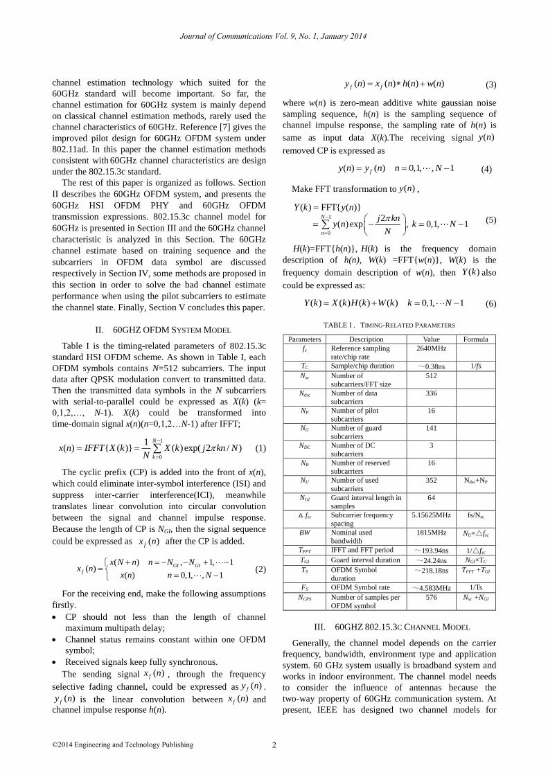
Table I is the timing-related parameters of 802.15.3c

standard HSI OFDM scheme. As shown in Table I, each

OFDM symbols contains N=512 subcarriers. The input

data after QPSK modulation convert to transmitted data.

Then the transmitted data symbols in the N subcarriers

with serial-to-parallel could be expressed as X(k) (k=

0,1,2,…, N-1). X(k) could be transformed into

time-domain signal x(n)(n=0,1,2…N-1) after IFFT;

1

0

1( ) { ( )} ( )exp( 2 / )

N

k

x n IFFT X k X k j kn NN

(1)

The cyclic prefix (CP) is added into the front of x(n),

which could eliminate inter-symbol interference (ISI) and

suppress inter-carrier interference(ICI), meanwhile

translates linear convolution into circular convolution

between the signal and channel impulse response.

Because the length of CP is NGI, then the signal sequence

could be expressed as ( )fx n after the CP is added.

( ) , 1, 1( )

( ) 0,1, , 1

GI GI

f

x N n n N Nx n

x n n N

(2)

For the receiving end, make the following assumptions

firstly.

CP should not less than the length of channel

maximum multipath delay;

Channel status remains constant within one OFDM

symbol;

Received signals keep fully synchronous.

The sending signal ( )fx n , through the frequency

selective fading channel, could be expressed as ( )fy n .

( )fy n is the linear convolution between ( )fx n and channel impulse response h(n).

( ) ( ) ( ) ( )f fy n x n h n w n (3)

where w(n) is zero-mean additive white gaussian noise

sampling sequence, h(n) is the sampling sequence of

channel impulse response, the sampling rate of h(n) is

same as input data X(k).The receiving signal ( )y n

removed CP is expressed as

( ) ( ) 0,1, , 1fy n y n n N (4)

Make FFT transformation to ( )y n ,

1

0

( ) FFT{ ( )}

2 ( )exp , 0,1, 1

N

n

Y k y n

j kny n k N

N

(5)

H(k)=FFT{h(n)}, H(k) is the frequency domain

description of h(n), W(k) =FFT{w(n)}, W(k) is the

frequency domain description of w(n), then ( )Y k also

could be expressed as:

( ) ( ) ( ) ( ) 0,1, 1Y k X k H k W k k N (6)

TABLE I . TIMING-RELATED PARAMETERS

Parameters Description Value Formula

fs Reference sampling

rate/chip rate

2640MHz

TC Sample/chip duration ～0.38ns 1/fs

Nsc Number of

subcarriers/FFT size

512

Ndsc Number of data subcarriers

336

NP Number of pilot

subcarriers

16

NG Number of guard

subcarriers

141

NDC Number of DC

subcarriers

3

NR Number of reserved subcarriers

16

NU Number of used

subcarriers

352 Ndsc+NP

NGI Guard interval length in samples

64

△ fsc Subcarrier frequency

spacing

5.15625MHz fs/Nsc

BW Nominal used bandwidth

1815MHz NU×△fsc

TFFT IFFT and FFT period ～193.94ns 1/△fsc

TGI Guard interval duration ～24.24ns NGI×TC

TS OFDM Symbol

duration ～218.18ns TFFT +TGI

FS OFDM Symbol rate ～4.583MHz 1/Ts

NCPS Number of samples per

OFDM symbol

576 Nsc +NGI

III. 60GHZ 802.15.3C CHANNEL MODEL

Generally, the channel model depends on the carrier

frequency, bandwidth, environment type and application

system. 60 GHz system usually is broadband system and

works in indoor environment. The channel model needs

to consider the influence of antennas because the

two-way property of 60GHz communication system. At

present, IEEE has designed two channel models for

Journal of Communications Vol. 9, No. 1, January 2014

2©2014 Engineering and Technology Publishing

60GHz, that is 802.15.3c and 802.11ad, and the two

models descript the signal propagation characteristics for

60GHz communication system. In 2009, the IEEE TG3c

working group released MAC layer and physical layer

standard for high speed wireless networks (WPANs) and

gave the channel model of 60 GHz wireless

communication system. This model is based on a lot of

measured data and statistical analysis [8]-[13], which

suitably described the large-scale fading and small-scale

fading characteristics for 60GHz wireless channel. In this

paper, the channel estimation design scheme is based on

802.15.3c standard. And the application environment is

based on 802.15.3c 60GHz channel model.

TABLE II . CM1 AND CM2 CHANNEL PARAMETER

Residential

LOS(CM1) NLOS(CM2)

TX360。

RX 15。

(CM1.1)

TX30。 RX

15。

(CM1.3)

TX360。

RX 15。

(CM2.1)

TX30。 RX

15。

(CM2.3)

/(1/ ns) 0.191 0.144 0.191 0.144

/(1/ ns) 1.22 1.17 1.22 1.17

/ ns 4.26 21.50 4.26 21.50

/ ns 6.25 4.35 6.25 4.35

/ dBc 6.28 3.71 6.28 3.71

/ dB 13.00 7.31 13.00 7.31

/() 49.8 46.2 49.8 46.2

L 9 8 9 8

k/dB 18.8 11.9 18.8 11.9

(d)/dB -88.7 -111.0 -88.7 -111.0

nd 2 2 2 2

ANLOS 0 0 0 0

In order to present the 60 GHz channel characteristics

accurately, this paper further employs two kinds of indoor

living environment channels model recommended by

TG3c and carries out the channel characteristics

simulation. That are indoor LOS channel (CM1) and

indoor NLOS channel (CM2) respectively. Table II is the

CM1 and CM2 channel parameter list.

Excess delay spread indicates the effective duration of

channel impulse response. It is the essential parameter

which judges the existence of ISI in OFDM system. If it

is shorter than the duration of protection interval, it will

not generate ISI in the demodulation process, otherwise,

it will generate ISI. The cyclic prefix length(which equal

to the length of protection interval) is set as 24.24ns for

60GHz OFDM system by 802.15.3c standard. If excess

delay is larger than this length, it is easier to generate ISI.

Fig. 1 is the 60GHz LOS and NLOS channel excess delay

spread simulation represented by CM1.1, CM1.3, CM2.1

and CM2.3 respectively, where the red dotted line shows

the 100 times average excess delay. The excess delay of

LOS channel is smaller than NLOS channel from the

simulation results. The 100 times average excess delay

simulation is about 0.01ns in CM1.1 channel, 0.08ns in

CM1.3 channel, 21.55ns in CM2.1 channel, 28.4ns in

CM2.3 channel. The differences of excess delay between

CM1.1 and CM1.3, CM2.1 and CM2.3 are caused by the

different half power beam width (HPBW) of transmission

signal.

0 10 20 30 40 50 60 70 80 90 1000

0.2

0.4

0.6

0.8

1

1.2

1.4

1.6

1.8x 10

-10 Excess delay (ns)

Channel number CM1.1

0 10 20 30 40 50 60 70 80 90 1000

0.2

0.4

0.6

0.8

1

1.2

1.4

1.6x 10

-9 Excess delay (ns)

Channel number CM1.3

0 10 20 30 40 50 60 70 80 90 1000

1

2

3

4

5

6

7x 10

-8 Excess delay (ns)

Channel number CM2.1

0 20 40 60 80 1000

1

2

3

4

5

6

7

8x 10

-8 Excess delay (ns)

Channel number CM2.3

Fig. 1. 100 times excess delay spread simulation of 802.15.3c

residential LOS and NLOS channel(CM1.1,CM1.3,CM2.1,CM2.3

respectively)

Journal of Communications Vol. 9, No. 1, January 2014

3©2014 Engineering and Technology Publishing

The discrete channel impulse response could reflect

the channel characteristics more clearly. Fig. 2 shows that

the power of LOS channel (represented by CM1.3) is

concentrated in the first arriving path. The multipath

phenomenon of NLOS channel (represented by CM2.3)

is more obvious, and energy is relatively dispersed. The

strongest energy path is not the first arriving path.

0 0.5 1 1.5 2 2.5 3 3.5 4 4.5

x 10-8

-40

-35

-30

-25

-20

-15

-10

-5

0Normalized Impulse Response Magnitude

nS

dB

0 1 2 3 4 5

x 10-8

-40

-35

-30

-25

-20

-15

-10

-5

0Normalized Impulse Response Magnitude

nS

dB

Fig. 2. The discrete channel impulse response of 802.15.3c channel(CM1.3 and CM2.3 respectively)

The discrete channel impulse response could reflect

the channel characteristics more clearly. Fig. 2 shows that

the power of LOS channel (represented by CM1.3) is

concentrated in the first arriving path. The multipath

phenomenon of NLOS channel (represented by CM2.3)

is more obvious, and energy is relatively dispersed. The

strongest energy path is not the first arriving path.

802.15.3c channel could use the cluster arriving model

recommended by TG3c and could be expressed as:

1 1

,kLK

kl k kl k klk l

h t t T

(7)

where δ(·) expresses impulse function, K expresses the

number of cluster arriving the receiver, kL expresses the

number of multipath in the kth cluster. kl , kl and

kl express the plural amplitude value, delay and arrival

angle in the kth cluster, lth path respectively. kT and

k express the delay and arrival angle in the kth cluster.

This model is the traditional S-V model which extends

to angle domain. Expression is complex, so it is

inconvenient to analyze and simulate. In this paper, the

model is simplified, unify the meaning of clusters and

multipath. All the signals at the receiver are identified as

multipath component which through the different time

delay and attenuation. In addition, the multipath gain

caused by azimuth angle is incorporated into the

variable kl . The model is simplified and expressed as

1

( )L

l ll

h t t t t

(8)

where l t is a plural which reflect the gain causing

by multipath, arrival angle, and antenna configuration, it's

modulo indicates the amplitude attenuation of lth path,

and it’s phase indicates the phase information of lth path.

( )l t indicates the additional delay of the lth path. L

indicates the total number of multipath reaching the

receiver. Each path has own delay, phase shift and gain.

The linear superposition of all paths constitutes the

channel impulse response. 60GHz wireless

communication system receiver has excellent multipath

resolution, if the system bandwidth is 5GHz, the

multipath resolution of the receiver will be 0.2ns.

According to the parameters given by TG3c, the

multipath average interval of 60GHz channel is greater

than 0.2ns. Take CM2 NLOS indoor channel for example,

the average interval of clusters is 5.24 ns, the average

interval of multipath in clusters is 0.82 ns [14]. Obviously,

each multipath can be distinguished on the receiver

basically.

The formula (8) could be expressed as after sampling:

1

( )N

n

h l n l n

(9)

where N is the total sampling points, which is the total

number of sampling tap delay line in discrete-time

channel.

IV. 60GHZ CHANNEL ESTIMATION TECHNIQUE

There are two basic channel estimation[15] methods in

OFDM systems which are illustrated in Fig. 3. The first

one, block-type pilot channel estimation, is developed

under the assumption of slow fading channel. The

multiple continuous OFDM symbols are divided into

groups (frames). One or several OFDM symbols in the

front of each group transmits pilot signal and all the

subcarriers of these OFDM symbols are used for channel

estimation. The remaining OFDM symbols in one

frame transmit data information. The second one,

comb-type pilot channel estimation, is introduced to

satisfy the need for equalizing when the channel status

changed. A few of pilot signals are inserted into each

OFDM symbol and partial subcarriers are used

for channel estimation. The channel estimation

characteristics of non pilot subcarriers depend on the

Journal of Communications Vol. 9, No. 1, January 2014

4©2014 Engineering and Technology Publishing

channel characteristics of pilot subcarriers through

interpolation in comb-type pilot channel estimation.

These two basic types are adopted in the 802.15.3c

OFDM scheme. Training sequence is inserted into the

beginning of each frame for channel estimation

(block-type pilot channel estimation), and the channel

estimation result is used in the following data symbols for

the whole frame. At the same time 16 pilot signals is

inserted in each OFDM data symbol of this frame

(comb-type pilot channel estimation) [4]. If the channel

status changes in the duration of one frame, comb-type

pilot channel estimation will be employed. In the

following research and simulation, we will use these two

estimation methods for 60 GHz channel estimation.

Fig. 3. Two basic types OFDM channel estimations

A. Channel Estimation based on Training Sequence

In the 802.15.3c standard, the training sequence

belongs to the PHY preamble. PHY Preamble locates in

the front of frame header, whose tasks are the frame

detection, frequency recurrence, frame synchronization

and channel estimation and so on [4], the structure of HSI

physical frame is demonstrated in Table III. The length of

preamble symbol equals to the length of FFT (512) in

OFDM system.

TABLE III . THE FRAME STRUCTURE OF HSI PHYSICAL

PHY

Preamble

Frame header Payload

PHY header MAC header HCS

The channel estimation method based on training

sequence employs all the 512 subcarriers of PHY

Preamble for channel estimation and the acquired channel

estimation result is used in the following data symbols

for the whole frame. Two kinds of channel estimation

algorithms based on training sequence are introduced in

the next section. The two algorithms are suitable for

60GHz channel characteristics.

1) 60GHz OFDM channel estimation algorithm based

on least square method (LS)

60GHz OFDM system uses N = 512 points FFT, X(k)

indicates the data within the OFDM symbol, which

contains the data signals and pilot signals. The received

signal Y at the receiver is a 1N vector:

0Y = XH N (10)

where N N matrix ( (1), (2), , ( )),diag X X X NX

1N vector H is the sampling values of frequency

domain channel response impulse. 1N vector 0N is

noise vector. LS algorithm [16] is the most common algorithm of

channel estimation. When using the training sequences of

each frame to estimate channel, the LS estimation is

expressed as:

( ) ( ) / ( ) ( ) ( )LSH k Y k X k H k W k (11)

where ( ) ( ) / ( )W k W k X k . Make IDFT to ( )LSH k

and get the time domain channel response impulse

representation ( ) { ( )}LS LSh n IFFT H k . The length of

( )LSh n is equal to the length of ( )LSH k , so it is 512.

Without using any priori information of the channels, the

LS estimators are calculated with very low complexity.

But it ignores the additive noise in the estimation process,

so LS algorithm is sensitive for the influence of noise

disturbance.

There is another basic channel estimation method,

minimum mean square error (MMSE) algorithm[17]. The

estimation precision is higher than LS algorithm. But this

algorithm needs to obtain the autocorrelation function of

current frequency domain channel impulse response and

needs to take matrix inversion. 60GHz OFDM system

needs 512512 matrix inversions. The complexity is too

high, and obtaining the autocorrelation function of

frequency domain channel impulse response is not very

easy, so this kind of estimation algorithm is not very

suitable for 60GHz channel estimation.

2) 60GHz OFDM channel estimation algorithm based

on DFT

As shown in Table I, the sampling interval of HSI

OFDM system is about 0.38ns, so the total sampling

duration of 512 points is about 218.18 ns. As shown in

figure 2, channel impulse response is basically

concentrated in the first 20ns in 60GHz LOS channel,

multipath energy has become very weak after 20ns

(CM1.1 channel impulse response is more concentrated,

focuses on the first few sampling points). Meanwhile

NLOS channel is basically concentrated in the first

60ns(about first 160 sampling points). The LS channel

estimation is continuous throughout the 512 sampling

points, so the length of estimated time has greatly

surpassed the duration of 60GHz channel impulse

response. The estimated value which exceed the duration

of 60GHz channel impulse response could be considered

pilot

data

Time

Block-type pilot estimation

Comb-type pilot estimation

Frequ

ency

Time

Frequ

ency

Journal of Communications Vol. 9, No. 1, January 2014

5©2014 Engineering and Technology Publishing

as noise, could be expressed as

( ) 0,1, , 1 ( )

( ) , 1, , 1

LS

LS

h n n Lh n

w n n L L N

(12)

where L is effective sampling value of time-domain

channel. Thus only the first L points contained useful

estimated channel information, the rest of the N-L points

only contain noise information. The DFT channel

estimation algorithm uses this characteristic. First using

LS estimation algorithm and get the channel transfer

function ( )LSH k , then ( )LSH k is processed by IDFT

and get ( )LSh n . The value of sampling point which

greater than L in the channel impulse response is set to 0.

And it is equivalent to using a simple L length window.

We could select Hamming window, Kaiser window and

Rectangular window, etc. This algorithm compensates

the effects of channel noise to some extent, especially in

the condition of low SNR, DFT channel estimation

algorithm have more obvious effect. In this paper we

select the rectangular window in the simulation and could

be expressed:

( ) 0,1, , 1 ( )

0 , 1, , 1

LS

LS

h n n Lh n

n L L N

(13)

Finally, transform ( )LSh n to frequency domain with

N points DFT, expressed as

( ) ( )DFT LSH k DFT h n . (14)

Assume W as N dimension DFT transformation matrix

00 ( 1)0

0( 1) ( 1)( 1)

1

N

N N N

WN

(15)

where ( )( ) 2 /n k j nk Ne .set L LI as L L unit matrix,

0

0 0

L LIQ = , Q is 512 512 matrix, so the DFT

channel estimation algorithm in frequency domain also could be written as

H

DFT LSH WQW H (16)

Transforming DFTH to time domain and getting the

time domain channel estimation DFTh .

Because there are 9 kinds of different channel models

in 802.15.3c channel model, the size L of rectangular

window should be selected according to the different

channel environments. Generally, the performance of

channel estimation algorithm is measured through

symbol error rate (SER) and mean square error (MSE).

where ˆ ˆ{ [( ) ( ) ]}HMSE trace E H H H H , H is the

estimated frequency domain channel impulse response,

and H is the actual frequency domain channel impulse

response, ( )trace indicates matrix trace. The duration of

channel impulse response is generally less than the

duration of cyclic prefix (CP) in LOS channel(the

duration of CP is 24.24ns). The orthogonality has been

kept between subcarriers when the duration of channel

impulse response is smaller than the duration of CP, and

the MSE of channel estimation will not increase

obviously. So the value of L could be considered as the

length of CP (64) for LOS channel. While the duration of

channel impulse response is far less than the duration of

CP(24.24ns) in CM1.1 channel. In order to get a better

channel estimation, L could be defined smaller than 64.

In this paper we set L = 64 and L = 10 respectively in the

LOS channel simulation. The duration of channel

impulse response is larger than 24.24ns in NLOS channel

in most cases. If set L=64 or L<64, it is likely to cause the

energy loss of partial multipath in the estimation process

and led to the poor performance in channel estimation.

performance of DFT algorithm (L=64) are both better

than LS algorithm, DFT (L=10) is better than DFT(L=64)

in CM1.1 channel. This is because the multipath

phenomenon is not obvious in CM1.1 channel. Most of

the energy is concentrated in the first few sampling points.

So the value of L is smaller, the possibility of filtering out

the noise is bigger.

0 2 4 6 8 10 12 1410

-5

10-4

10-3

10-2

10-1

100

SNR(dB)

SE

R

LS Channel Estimation SER

DFT Channel Estimation SER L=10

DFT Channel Estimation SER L=64

0 2 4 6 8 10 12 14 16 1810

-4

10-3

10-2

10-1

100

101

SNR(dB)

MS

E

LS Estimation MSE

DFT Estimation MSE L=10

DFT Estimation MSE L=64

Fig. 4. SER and MSE performance comparison between LS channel

estimation and DFT channel estimation in CM1.1 channel

Journal of Communications Vol. 9, No. 1, January 2014

6©2014 Engineering and Technology Publishing

As shown in Fig. 4 whether the SER or MSE

Fig. 5 presents the simulation result in NLOS channel

represented by CM2.3. The energy of multipath is

average in this channel, energy is not mainly

concentrated in the first arriving path. The duration of

channel impulse response is generally close to or greater

than the duration of CP, and it is prone to generate

inter-symbol interference (ISI) at this time. The

simulation result shows that the accuracy of channel

estimation is very poor when L less than or equal to the

length of CP in NLOS channel. That is because the

channel energy is not concentrate in the duration of CP,

at this moment still using L=64 DFT algorithm for

channel estimation will cause high BER. The duration of

channel impulse response is generally within 2 times

duration of CP in NLOS channel. So the value of L could

be set as 128 for NLOS channel. The simulation

comparison between DFT (L=128) algorithm and DFT

(L=256) algorithm tests the rationality of L. The DFT

(L=256) algorithm have contained all the energy of

channel impulse response, while at the same time it

brings excess noise and reduces the accuracy of

estimation. Under the NLOS channel, the DFT algorithm

L=128 and L=256 are both superior to the LS algorithm

channel estimation.

0 2 4 6 8 10 12 14 16 1810

-4

10-3

10-2

10-1

100

SNR(dB)

SE

R

LS Channel Estimation SER

DFT Channel Estimation SER L=128

DFT Channel Estimation SER L=256

DFT Channel Estimation SER L=64

0 2 4 6 8 10 12 14 16 1810

-3

10-2

10-1

100

101

SNR(dB)

MS

E

LS Estimation MSE

DFT Estimation MSE L=128

DFT Estimation MSE L=256

DFT Estimation MSE L=64

Fig. 5. SER and MSE performance comparison between LS channel estimation and DFT channel estimation in CM2.3 channel

B. Channel Estimation based on Pilot Subcarriers

If the channel is time-invariant channel during the

whole period of one frame, training sequence estimation

methods could be used. That is to say OFDM data

symbols in each frame could use the channel estimated

value by the training sequence if the channel condition

have not changed. 60GHz channel usually belongs to

time-invariant channel, however, each frame signal may

last several hundred milliseconds in reality, so the

channel status may change during this time. In 802.15.3c

standard, the largest number of transmitted OFDM

symbol per frame is 1024 and the duration of each

OFDM symbol is 218.18ns [4]. The longest duration of

data OFDM symbols after the training sequence is

218.18ns*1024=223ms in one frame. While 60GHz

signal is sensitive to block and relative movement

between transmitter and receiver, so it is probable that the

channel condition changes in one frame. It may appear

huge deviation and cause the performance decreasing if

only using the training sequence channel estimation

method.

The simulation results in Fig. 6 verify the validity of

above consideration. When the channel status changes

from LOS channel (CM1.3) to NLOS channel (CM2.3),

the system SER performance comparison between using

the preceding CM1.3 channel status and the correct

CM2.3 channel status by training sequence is presented

in this figure. The estimation result of training sequence

located in the front of each frame and corresponding to

LOS channel status while the OFDM data signals after

the training sequence corresponding to NLOS channel. If

still using the estimated channel status in LOS channel,

the SER performance will be very large.

0 2 4 6 8 10 12 14 16 1810

-4

10-3

10-2

10-1

100

SNR(dB)

SE

R

LS Channel Estimation SER

LS Channel Estimation SER change

DFT Channel Estimation SER

Fig. 6. SER performance simulation when the channel condition changing while the estimate method does not change timely

When the channel status suddenly changes, channel

estimation can't adjust in time when using training

sequence and lead to the bad performance. Regard to this

problem, we could using the pilot signals to estimate the

channel status in each OFDM symbol and get the channel

status of current OFDM symbol. The estimation method

based on pilot subcarriers has two steps: first using an

algorithm, estimates the frequency channel impulse

response in the position of pilot subcarriers; then using

the Interpolation method to estimate the entire frequency

Journal of Communications Vol. 9, No. 1, January 2014

7©2014 Engineering and Technology Publishing

channel function H (k).

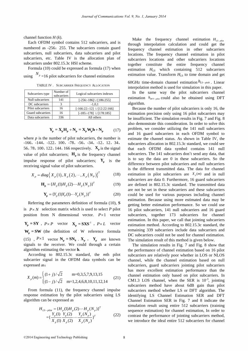
Each OFDM symbol contains 512 subcarriers, and is

numbered as -256：255. The subcarriers contain guard

subcarriers, null subcarriers, data subcarriers and pilot

subcarriers, etc. Table IV is the allocation plan of

subcarriers under 802.15.3c HSI scheme.

Formula (10) could be expressed as formula (17) when

using pN=16 pilot subcarriers for channel estimation

TABLE IV . S

Subcarriers type Number of

subcarriers Logical subcarriers indexes

Null subcarriers 141 [-256:-186]∪[186:255]

DC subcarriers 3 -1,0,1

Pilot subcarriers 16 [-166:22:-12] ∪[12:22:166]

Guard subcarriers 16 [-185:-178] ∪[178:185]

Data subcarriers 336 All others

p p p p p p pY = X H N = X W h N (17)

where p is the number of pilot subcarriers, the number is -166，-144，-122，100，-78，-56，-34，-12，12，34，

56，78，100，122，144，166 respectively. pX is the signal

value of pilot subcarriers; pH is the frequency channel

impulse response of pilot subcarriers; pY is the

receiving signal value of pilot subcarriers.

{ (1) (2) ( )}T

p p p pH H H NpH (19)

{ (1) (1) ( )}T

p P p pY Y Y NpY (20)

Referring the parameters definition of formula (10), S

is P N selection matrix which is used to select P pilot

position from N dimensional vector. 1P vector

pY = SY , P P vector -1

pX = SXS , P L vector

pW = SW (the definition of W reference formula

(15) , 1P vector p 0N = SN . pX ， pY are known

signals to the receiver. We could through a certain

algorithm estimating the vector h.

According to 802.15.3c standard, the mth pilot

subcarrier signal in the OFDM data symbols can be

expressed as：

(1 ) / 2 m=0,3,5,7,9,13,15( )

(1 ) / 2 m=1,2,4,6,8,10,11,12,14p

jX m

j

(21)

From formula (11), the frequency channel impulse

response estimation by the pilot subcarriers using LS

algorithm can be expressed as

{ (1) (2) ( )}

(1) (2) ( ) ={ }

(1) (2) ( )

T

LS pilot p p p p

p p p p T

p p p p

H H H H N

Y Y Y N

X X X N

(22)

Make the frequency channel estimation LS pilotH

through interpolation calculation and could get the

frequency channel estimation in other subcarriers

locations. The frequency channel estimation in pilot

subcarriers locations and other subcarriers locations

together constitute the entire frequency channel

estimation HLS which containing 512 subcarriers

estimation value. Transform HLS to time domain and get

60GHz time-domain channel estimation LS piolth . Linear

interpolation method is used for simulation in this paper.

In the same way the pilot subcarriers channel

estimation DFT piloth could also be obtained using DFT

algorithm.

Because the number of pilot subcarriers is only 16, the

estimation precision only using 16 pilot subcarriers may

be insufficient. The simulation results in Fig. 7 and Fig. 8

also demonstrate this consideration. In order to solve this

problem, we consider utilizing the 141 null subcarriers

and 16 guard subcarriers in each OFDM symbol to

estimate the channel status. As shown in Table IV, the

subcarriers allocation in 802.15.3c standard, we could see

that each OFDM data symbol contains 141 null

subcarriers. The 141 subcarriers don’t send any data, that

is to say the data are 0 in these subcarriers. So the

difference between pilot subcarriers and null subcarriers

is the different transmitted data. The data for channel

estimation in pilot subcarriers are ( )pX m and in null

subcarriers are data 0. Furthermore, 16 guard subcarriers

are defined in 802.15.3c standard. The transmitted data

are not be set in these subcarriers and these subcarriers

could be used for various purposes including channel

estimation. Because using more estimated data may be

getting better estimation performance. So we could use

16 pilot subcarriers, 141 null subcarriers and 16 guard

subcarriers, together 173 subcarriers for channel

estimation. In this paper, we call that jointing subcarriers

estimation method. According to 802.15.3c standard, the

remaining 339 subcarriers include data subcarriers and

DC subcarriers could not be used for channel estimation.

The simulation result of this method is given below.

The simulation results in Fig. 7 and Fig. 8 show that

the performance of channel estimation based on 16 pilot

subcarriers are relatively poor whether in LOS or NLOS

channel, while the channel estimation based on null

subcarriers, guard subcarriers jointing pilot subcarriers

has more excellent estimation performance than the

channel estimation only based on pilot subcarriers. In

CM1.3 LOS channel, when the SER is 10-3, jointing

subcarriers method have about 6dB gain than pilot

subcarriers method whether LS or DFT algorithm. The

identifying LS Channel Estimation SER and DFT

Channel Estimation SER in Fig. 7 and 8 indicate the

simulation result using entire 512 subcarriers (training

sequence estimation) for channel estimation, In order to

contrast the performance of jointing subcarriers method,

we introduce the ideal entire 512 subcarriers for channel

Journal of Communications Vol. 9, No. 1, January 2014

8©2014 Engineering and Technology Publishing

UBCARRIER REQUENCY LLOCATIONF A

(18) 1 , 2 , ,T

p p p p PX diag X X X N

estimation method. The channel estimation performance

based on jointing subcarriers is closed to the performance

based on entire 512 subcarriers estimation. The reason for

this result is that the multipath phenomenon is not

obvious in CM1.3 channel and most of the energy is

concentrated in the first few sampling points. Using only

16 pilot subcarriers data could not estimate the complete

channel status at this time, while the estimation method

based on jointing subcarriers estimation could satisfy the

demand of channel estimation. So this method could get

more excellent performance. In CM2.3 channel, the

jointing subcarriers method has significant advantage

than pilot subcarriers method whether using LS or DFT

algorithm. But there is a large performance gap between

the jointing subcarriers method and entire 512 subcarriers

estimation method in NLOS channel. This is because the

number of multipath is big and the channel status is more

complicated in NLOS channel. More data information are

needed for channel estimation. Null subcarriers, guard

subcarriers jointing pilot subcarriers still could not give a

complete estimation to the complex channel condition.

0 2 4 6 8 10 12 14 16 1810

-5

10-4

10-3

10-2

10-1

100

SNR(dB)

SE

R

LS Channel Estimation SER (512subcarriers )

DFT Channel Estimation SER (512subcarriers )

LS Channel Estimation SER (16 pilot subcarriers)

DFT Channel Estimation SER(16 pilot subcarriers)

LS Channel Estimation SER pilot+Null+Guard subcarriers

DFT Channel Estimation SER pilot+Null+Guard subcarriers

Fig. 7. The SER performance comparison between jointing estimation and 16 pilot subcarriers estimation in CM1.3 channel (DFT length

L=10)

0 2 4 6 8 10 12 14 16 1810

-4

10-3

10-2

10-1

100

SNR(dB)

SE

R

LS Channel Estimation SER (512 subcarriers)

DFT Channel Estimation SER(512 subcarriers)

LS Channel Estimation SER (16 pilot subcarriers)

DFT Channel Estimation SER (16 pilot subcarriers)

LS Channel Estimation SER pilot+Null+Guard subcarriers

DFT Channel Estimation SER pilot+Null+Guard subcarriers

Fig. 8. The SER performance comparison between jointing estimation

16 pilot subcarriers estimation in CM2.3 channel(DFT length L=128)

C. Channel Estimation based on Compressed Sensing

Orthogonal Matching Pursuit Method

As shown in Fig. 8, whether jointing pilot subcarriers

estimation or only pilot subcarriers estimation both could

not get good estimation performance in NLOS channel.

So a better NLOS channel estimation method which

could uses limited OFDM subcarriers data and gets better

estimation performance should be search. As shown in

Fig. 2 whether in LOS or NLOS channel, 60GHz channel

impulse response show sparse characteristic in time

domain. The sparse characteristic in 60GHz channel is

reflected that the number of nonzero elements or greater

value elements is relatively small and the number of zero

elements or closing to zero elements is relatively big in

( )n of formula (10). In traditional signal processing

methods, Nyquist sampling is an important premise for

correct recovery of signal at the receiver. In order to get

better channel estimation performance, only take

advantage of enough subcarriers could obtain more

complete estimation result for 60GHz OFDM system.

While the compressed sensing (CS) theory proposed by

Candes, Tao [18] and Donoho [19] demonstrate that

using fewer measurements could recover the information

of signals when the signals are sparse or compressible. So

when the pilot signals for channel estimation are not

enough, CS theory provides a new solution and makes it

possible to have better channel estimation performance

while using fewer estimation subcarriers.

Now, the basic principle of CS theory is illustrated firstly. Assume a discrete time signal x（the length is

1N ）and whose transform coefficient α is sparse in ψ domain,

x ψα (23)

where ψ is a base vector which located in same space

with x, α is the projection coefficient of signal x in ψ

domain, that is the ψ domain expression of x. If could find an observation matrixΦwhich not related with base

vector ψ (Φ is M N matrix, M＜＜N). Making the

linear transformation to signal x, we could obtain the observation vector y(y is 1M matrix).

y Φx Φψα (24)

The original signal could be high probability of

reconstruction using optimization algorithm from

observation vector. Defined M/N as compression rate,

which is the ratio of CS sampling rate to Nyquist

sampling rate. If the signal x could be sparse

representation or be compressed, the problem of solving

formula (24) could be converted into minimum 0 norm

problem. But this is a NP hard problem. Paper [20]

indicated that solving a simpler minimum l1 norm

optimization problem will produce the same solution, so

the problem is transformed into

1min s.t. α y =Φψα , (25)

the reconstruction problem of signals containing noise

also can be converted to the minimum l1 norm problem,

1min s.t. α Φψα - y . (26)

The basis pursuit (BP) algorithm[21], Matching

Pursuit(MP) algorithm[20], Orthogonal Matching Pursuit

Journal of Communications Vol. 9, No. 1, January 2014

9©2014 Engineering and Technology Publishing

(OMP) algorithm[22] could be used to solve the problem

of formula (26). This paper will use the basic principle of

CS theory and the representative OMP restoration

algorithm to complete 60GHz channel estimation

simulation. The basic idea of OMP algorithm is that

select the best match atom to approximate the

observation vector from over-complete dictionary

(over-complete dictionary is restore matrix T ΦΨ ).

Working out the residual signal, then select the most

matching atoms with residual signal. After a certain

number of iterations, signals could be linear expression

by some atoms. The selected atoms are made

orthogonalization when using OMP algorithm. OMP

algorithm ensures the optimality of the iteration and

reduces the number of iterations.

The methods and steps of sparse channel estimation

using the OMP algorithm are described below.

Supposing the observation vector MCy , the

estimated sparse channel impulse response NCh ,

restore matrix , M NC p pT = X W T , sampling noise

vector MCz . y and T are known vector at the receiver. According to CS theory, formula (27) could be obtained

y = Th z (27)

Contrast formula (17) and (27), the corresponding

relation is that ,py = Y ,p pT = X W pz = N .

The purpose of OMP channel estimation algorithm is

recovering the sparse vector h, which is to find the

location and value of nonzero element in h. Since the

orthogonality between subcarriers in OFDM system, the

atoms in over-complete dictionary (restore matrix

p pT = X W ) are orthogonal. So to OFDM system,

Gram-Schmidt orthogonalization is not needed, which

reduces the computational complexity of OMP channel

estimation algorithm.

The steps of OMP channel estimation algorithm are

described as below:

Initializing the program, iterations j =0, residual r0=y,

index collection 0S .

when 1,2,...j ,confirm the position of

index js , js should satisfy the formula

1

1 1{1, , }\

, max ,j

jj s j s

s N sr r

, where s indicates the

sth column vector of matrix T.

Fill js to index collection 1 { }j j jS S s .

Obtain the channel estimation value |ˆ

jj sh in the

position of js using LS algorithm,

21

|ˆ arg min{ }

j

j

j sh s

h

j js sy T h T y

, the values outside

the index collection are set as 0. Where

jsTis M j dimension matrix and contains all the

columns which the index are jS in restore matrix T.

From formula ˆ ˆ

j jj j s j|sy = Th = T h , j jr = y y ,

update the observation vector and residuals. If the

predetermined iterations J is smaller than j or meets

the requirements of approximation error, the iteration

stops. Else jump to step (2).

After J times iterations, obtain the J sparse vector h .

0 2 4 6 8 10 12 14 16 1810

-5

10-4

10-3

10-2

10-1

100

SNR(dB)S

ER

CS Estimation SER(512 subcarriers)

LS Estimation SER(512 subcarriers)

DFT Estimation SER(512 subcarriers)

CS Estimation SER pilot+Null+Guard suarriers

LS Estimation SER pilot+Null+Guard subcarriers

DFT Estimation SER pilot+Null+Guard subcarriers

CS Estimation SER(16 pilot sucarriers)

LS Estimation SER (16 pilot sucarriers)

DFT Estimation SER (16 pilot sucarriers)

Fig. 9. The SER performance comparison among CS OMP channel

estimation algorithm, LS channel estimation algorithm, DFT channel estimation algorithm in CM1.3 channel(DFT estimation length L=10)

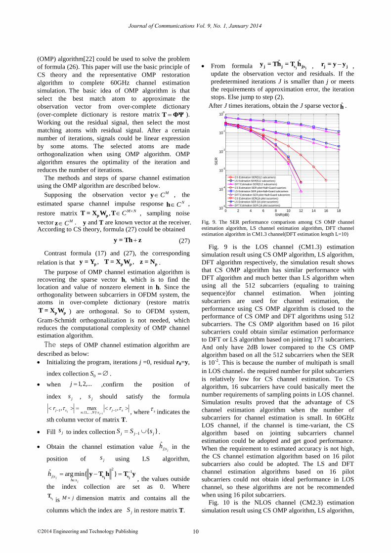
Fig. 9 is the LOS channel (CM1.3) estimation

simulation result using CS OMP algorithm, LS algorithm,

DFT algorithm respectively, the simulation result shows

that CS OMP algorithm has similar performance with

DFT algorithm and much better than LS algorithm when

using all the 512 subcarriers (equaling to training

sequence)for channel estimation. When jointing

subcarriers are used for channel estimation, the

performance using CS OMP algorithm is closed to the

performance of CS OMP and DFT algorithms using 512

subcarriers. The CS OMP algorithm based on 16 pilot

subcarriers could obtain similar estimation performance

to DFT or LS algorithm based on jointing 171 subcarriers.

And only have 2dB lower compared to the CS OMP

algorithm based on all the 512 subcarriers when the SER

is 10-2

. This is because the number of multipath is small

in LOS channel，the required number for pilot subcarriers

is relatively low for CS channel estimation. To CS

algorithm, 16 subcarriers have could basically meet the

number requirements of sampling points in LOS channel.

Simulation results proved that the advantage of CS

channel estimation algorithm when the number of

subcarriers for channel estimation is small. In 60GHz

LOS channel, if the channel is time-variant, the CS

algorithm based on jointing subcarriers channel

estimation could be adopted and get good performance.

When the requirement to estimated accuracy is not high,

the CS channel estimation algorithm based on 16 pilot

subcarriers also could be adopted. The LS and DFT

channel estimation algorithms based on 16 pilot

subcarriers could not obtain ideal performance in LOS

channel, so these algorithms are not be recommended

when using 16 pilot subcarriers.

Fig. 10 is the NLOS channel (CM2.3) estimation

simulation result using CS OMP algorithm, LS algorithm,

Journal of Communications Vol. 9, No. 1, January 2014

10©2014 Engineering and Technology Publishing

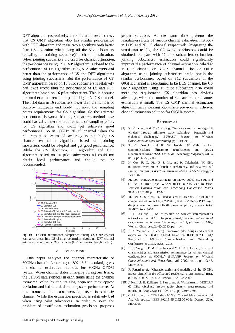
DFT algorithm respectively, the simulation result shows

that CS OMP algorithm also has similar performance

with DFT algorithm and these two algorithms both better

than LS algorithm when using all the 512 subcarriers

(equaling to training sequence)for channel estimation.

When jointing subcarriers are used for channel estimation,

the performance using CS OMP algorithm is closed to the

performance of LS algorithm using 512 subcarriers and

better than the performance of LS and DFT algorithms

using jointing subcarriers. But the performance of CS

OMP algorithm based on 16 pilot subcarriers is relatively

bad, even worse than the performance of LS and DFT

algorithms based on 16 pilot subcarriers. This is because

the number of nonzero multipath is big in NLOS channel.

The pilot data in 16 subcarriers lower than the number of

nonzero multipath and could not meet the sampling

points requirements for CS algorithm. So the estimate

performance is worst. Jointing subcarriers method have

could basically meet the requirements of sampling points

for CS algorithm and could get relatively good

performance. So in 60GHz NLOS channel when the

requirement to estimated accuracy is not high, CS

channel estimation algorithm based on jointing

subcarriers could be adopted and get good performance.

While the CS algorithm, LS algorithm and DFT

algorithm based on 16 pilot subcarriers all could not

obtain ideal performance and should not be

recommended.

0 2 4 6 8 10 12 14 16 1810

-4

10-3

10-2

10-1

100

SNR(dB)

SE

R

CS Estimation SER

LS Estimation SER

DFT Estimation SER

CS Estimation SER pilot+Null+Guard subcarriers

LS Estimation SER pilot+Null+Guard subcarriers

DFT Estimation SER pilot+Null+Guard subcarriers

CS Estimation SER pilot

LS Estimation SER pilot

DFT Estimation SER pilot

Fig. 10. The SER performance comparison among CS OMP channel

estimation algorithm, LS channel estimation algorithm, DFT channel estimation algorithm in CM2.3 channel(DFT estimation length L=128)

V. CONCLUSION

This paper analyzes the channel characteristic of

60GHz channel. According to 802.15.3c standard, gives

the channel estimation methods for 60GHz OFDM

system. When channel status changing during one frame,

the OFDM data symbols in each frame using the channel

estimated value by the training sequence may appear

deviation and led to a decline in system performance. At

this moment, pilot subcarriers are used to estimate

channel. While the estimation precision is relatively bad

when using pilot subcarriers. In order to solve the

problem of insufficient estimation precision, proposes

proper solutions. At the same time presents the

simulation results of various channel estimation methods

in LOS and NLOS channel respectively. Integrating the

simulation results, the following conclusions could be

obtained: compare with 16 pilot subcarriers estimation,

jointing subcarriers estimation could significantly

improve the performance of channel estimation. whether

in LOS channel or NLOS channel, The CS OMP

algorithm using jointing subcarriers could obtain the

similar performance based on 512 subcarriers. If the

60GHz channel is ascertained to be LOS channel, the CS

OMP algorithm using 16 pilot subcarriers also could

meet the requirement. CS algorithm has obvious

advantage when the number of subcarriers for channel

estimation is small. The CS OMP channel estimation

algorithm using jointing subcarriers provides an efficient

channel estimation solution for 60GHz system.

REFERENCES

[1] S. K. Yong and C.-C. Chong, “An overview of multigigabit

wireless through millimeter wave technology: Potentials and

technical challenges,” EURASIP Journal on Wireless

Communications and Networking, pp. 1-10, 2007.

[2] R. C. Daniels and R. W. Heath, “60 GHz wireless

communications: Emerging requirements and design

recommendations,” IEEE Vehicular Technology Magazine, vol. 2,

no. 3, pp. 41-50, 2007.

[3] N. Guo, R. C. Qiu, S. S. Mo, and K. Takahashi, “60 GHz

millimeter-wave radio: Principle, technology, and new results,”

Eurasip Journal on Wireless Communications and Networking, pp.

1-8, 2007.

[4] M. Lei, “Hardware impairments on LDPC coded SC-FDE and

OFDM in Multi-Gbps WPAN (IEEE 802.15.3c),” in Proc.

Wireless Communication and Networking Conference, March

31-April 3 2008, pp. 442.446

[5] M. Lei, C.-S. Choi, R. Funada, and H. Harada, “Through-put

comparison of multi-Gbps WPAN (IEEE 802.15.3c) PHY layer

designs under non-linear 60-GHz power amplifier,” in Proc. IEEE

PIMRC, Sept. 2007

[6] H. H. Xu and L. Ke, “Research on wireless communication

networks in the 60 GHz frequency band,” in Proc. International

Conference on Internet Technology and Applications (iTAP),

Wuhan, China, Aug 21-23, 2010, pp. 1-4.

[7] B. X. Ye and Z. C. Zhang. "Improved pilot design and channel

estimation for 60GHz OFDM based on IEEE 802.11. ad,"

Presented at Wireless Communications and Networking

Conference (WCNC), IEEE., 2013.

[8] H. B. Yang, P. F. M. Smulders, and M. H. A. J. Herben, “Channel

characteristics and transmission performance for various channel

configurations at 60GHz,” EURASIP Journal on Wireless

Communications and Networking, vol. 2007, no. 1, pp. 43-43,

March 2007.

[9] P. Pagani et al., “Characterization and modeling of the 60 GHz

indoor channel in the office and residential environments,” IEEE

802.15-06-0027-02-003c, Hawaii, USA, Jan 2006.

[10] J. Kunisch, E. Zollinger, J. Pamp, and A. Winkelmann, “MEDIAN

60 GHz wideband indoor radio channel measurements and

model,” in Proc. IEEE VTC’99, 1997, pp. 2393~2397.

[11] C. Liu, et al., “NICTA Indoor 60 GHz Channel Measurements and

Analysis update,” IEEE 802.15-06-0112-00-003c, Denver, USA,

Mar 2006.

Journal of Communications Vol. 9, No. 1, January 2014

11©2014 Engineering and Technology Publishing

Journal of Communications Vol. 9, No. 1, January 2014

12©2014 Engineering and Technology Publishing

[12] H. Sawada, Y. Shoji, and H. Ogawa, “NICT propagation data,”

IEEE 802.15.06-0012-01-003c, Hawaii, USA, Jan 2006.

[13] T. Zwick, T. J. Beukema, and H. Nam, “Wideband channel

sounder with measurements and model for the 60 GHz indoor

radio channel,” IEEE Trans. Vech. Technol. vol. 54, pp.

1266-1277, July 2005.

[14] IEEE 802.15 Working Group for WPAN [Online]. Available:

http://www.ieee802.org/15/

[15] J.-J. Van de Beek, et al., “On channel estimation in OFDM

systems,” in Proc. IEEE 45th Vehicular Technology Conference,

25-28 Jul 1995, vol. 2, pp. 815-819.

[16] S Haykin, “Cognitive radio: Brain empowered wireless

communi-cations,” IEEE Journal on Selected Areas In Commun,

vol. 23, no. 2, pp. 201-220, 2005.

[17] B. G. Yang, Z. G. Cao, and K. B. Lataief, “Analysis of

low-complexity windowed dte based mmse channel estimator for

OFDM system,” IEEE Transactions on Communications, vol. 49,

no. 11, pp. 1977-1987, 2001.

[18] E. Candes, J. Romberg, and T. Tao, “Robust uncertainty principles:

Exact signal reconstruction from highly incomplete frequency

information,” IEEE Trans. Inform. Theory, vol. 52, no. 2, pp.

489-509, Feb 2006.

[19] D. Donoho, “Compressed sensing,” IEEE Trans. Inform. Theory,

vol. 52, no. 4, pp. 1289-1306, April 2006.

[20] S. Chen, D. L. Donoho, and M. Saunders, “Atomic

Decomposition by Basis Pursuit,” SIAM Journal on Scientific

Computing, vol. 20, no. 1, pp. 33-61, 1999.

[21] R. G. Baraniuk, “Compressive sensing,” IEEE Signal Processing

Magazine, vol. 24, no. 4, pp. 118 - 120, 2007.

[22] S. G. Mallat and Z. Zhang, “Matching pursuit with time-frequency

dictionaries,” IEEE Trans on Signal Processing, vol. 41, no. 12,

pp. 3393- 3415, 1993.

Wei Shi was pursuing his Ph.D degree in

Ocean University of China now. He was born

in Shandong, China, in 1986. He received his

B.S. degree in Ludong University, Yantai,

China, in 2009, and the Master Degree in

Signal and Information processing from Ocean

University of China, China in 2011. From

2011 to now, he is a doctoral candidate of

department of electrical engineering, Ocean

University of China. His research interests include OFDM, MIMO, LTE,

UWB and 60 GHz wireless communication.

Hao Zhang

was born in Jiangsu, China, in

1975.

He received his Bachelor Degree in

Telecom Engineering

and Industrial

Management from Shanghai

Jiaotong

University, China in 1994, his MBA from

New

York Institute of Technology, USA in 2001,

and

his Ph.D. in Electrical and Computer

Engineering

from the University of Victoria,

Canada in 2004.

In 2000, he joined

Microsoft

Canada as a Software Engineer, and was Chief Engineer at Dream

Access Information Technology, Canada from 2001 to 2002. He is

currently

a

professor in the Department of Electrical Engineering

at the

Ocean University of China, and an

Adjunct Assistant Professor in the

Department of Electrical and Computer

Engineering at the University of

Victoria.

His research interests include UWB

wireless systems, MIMO

wireless systems, and spectrum

communications.

Xinjie Wang was pursuing his Ph.D degree in

Ocean University of China now. He was born

in 1980. He received his B.S. Degree in

Electrical and Information from Qufu Normal

University, China in 2003, and the Master

Degree in Signal and Information processing

from Sun Yat-sen University, China in 2005.

From 2005 to now, he is a

lecturer in College

of Communication and Electronics, Qingdao

Technological University. His research interests include cooperative

communication networks, cognitive radio networks, cross-layer design,

UWB

and digital communication over fading channels, etc.

Jingjing Wang was born in Anhui, China, in

1975. She received her B.S. degree in

Industrial Automation from Shandong

University, Jinan, China, in 1997, the M.Sc.

degree in Control Theory and Control

Engineering, Qingdao University of Science

& Technology, Qingdao, China, in 2002, and

the Ph.D. degree in Computer Application

Technology, Ocean University of China,

Qingdao, China, in 2012.

From 1997 to 1999, she was the assistant

engineer of Shengli Oilfield, Dongying, China. From 2002 to now, she

is an associate professor at the College of Information Science &

Technology, Qingdao University of Science & Technology. Her

research interests include 60

GHz wireless communication, 60

GHz

wireless position technology, ultra wideband radio systems, and

cooperative communication networks.

Hongjiao

Zhang

is pursuing the Ph.D. degree

at Ocean University of China. He received the

B.S. degree in Changchun University of

Science and Technology in 2006 and the

Master degree in Communication and

information System from Ocean University of

China in 2010. His research interests include

60GHz wireless communication and UWB

wireless communication.