Improved algorithm for the transmittanceestimation of spectra obtained withSOIR/Venus ExpressLOIC TROMPET,1,* ARNAUD MAHIEUX,1,2 BOJAN RISTIC,1 SÉVERINE ROBERT,1 VALÉRIE WILQUET,1

IAN R. THOMAS,1 ANN CARINE VANDAELE,1 AND JEAN-LOUP BERTAUX3

1Planetary Aeronomy, Royal Belgian Institute for Space Aeronomy, 3 Avenue Circulaire, 1180 Brussels, Belgium2Fonds National de la Recherche Scientifique, Brussels, Belgium3LATMOS/IPSL, Université Versailles St-Quentin, CNRS/INSU, 11 Boulevard d’Alembert, 78280 Guyancourt, France*Corresponding author: loic.trompet@aeronomie.be

Received 2 September 2016; revised 17 October 2016; accepted 17 October 2016; posted 18 October 2016 (Doc. ID 275012);published 9 November 2016

The Solar Occultation in the InfraRed (SOIR) instrument onboard the ESA Venus Express spacecraft, an infraredspectrometer sensitive from 2.2 to 4.3 μm, probed the atmosphere of Venus from June 2006 until December 2014.During this time, it performed more than 750 solar occultations of the Venus mesosphere and lower thermosphere.A new procedure has been developed for the estimation of the transmittance in order to decrease the number ofrejected spectra, to check that the treated spectra are well calibrated, and to improve the quality of the calibratedspectra by reducing the noise and accurately normalizing it to the solar spectrum. © 2016 Optical Society of America

OCIS codes: (120.6085) Space instrumentation; (120.6200) Spectrometers and spectroscopic instrumentation; (300.6340)

Spectroscopy, infrared; (010.0280) Remote sensing and sensors.

http://dx.doi.org/10.1364/AO.55.009275

1. INTRODUCTION

The SOIR (Solar Occultation in the InfraRed) spectrometer waspart of the scientific payload onboard the Venus Express (VEx)orbiter of the European Space Agency (ESA) [1,2]. The SOIRinstrument and its calibration have already been extensivelydescribed elsewhere [1,3–5], and only a summary will be givenhere. SOIR operated in the near infrared, being sensitive in the2.2–4.3 μm (2200 to 4370 cm−1) spectral range. It combinedan echelle grating in front of which an acousto-optical tunablefilter (AOTF) was placed for the selection of the spectral intervalrecorded. The spectral domain is divided in 94 regionscorresponding to the diffraction orders of the echelle grating(101–194). During a solar occultation observation, SOIR was ableto scan up to four orders, on a one second cycle basis. The SOIRdetector has 320 pixel columns along the wavenumber axis and256 pixels in the spatial direction, of which only 32 rows are il-luminated. Telemetry limitations implied that only 8 rows of320 pixels could be downlinked per second to Earth. For this rea-son, the pixel lines had to be binned onboard before being sent toEarth. Several binning schemes were used during the mission,varying the number of orders scanned and the number of binnedpixel rows. They are summarized in Table 1. For most of the mea-surements, four orders were scanned. In the beginning of themission, the rows were binned in 2 groups of 16 rows. After orbit

262, the rows were separated in 2 bins of 12 rows to avoid takinginto account the side rows, which were less illuminated.

Most of the solar occultation observations were made using2 bins of 12 rows, see Table 1. Measurements made using 4bins of 3 rows and 8 bins of 3 rows have not been used forsolar occultation observations but for other measurementsdedicated to calibration [3].

A solar occultation observation consists of measuring thesolar radiation passing through the atmosphere: during anorbit, an occultation occurs when the spacecraft passes behindthe planet with respect to the Sun, entering the planet’s shadow.Another occultation occurs when the spacecraft exits theshadow of the planet. These geometries are called ingress andegress, respectively. An egress is effectively identical to an in-gress if reversed in time. During an ingress, the recording ofspectra begins well before the line of sight of SOIR intersectsthe top layers of the atmosphere, which has arbitrarily beenfixed at a 220 km altitude. The spectra taken above this altitudeprovide a reference for the calculation of the transmittances.

Individual spectra are grouped by bin and diffraction orderfor each observation: throughout SOIR’s lifetime, 6232 of thesesets of spectra were measured during 3219 orbits of Venus dur-ing over eight years of operation. SOIR made 1468 valid mea-surements from 12 May 2006 to 27 November 2014. Among

Research Article Vol. 55, No. 32 / November 10 2016 / Applied Optics 9275

1559-128X/16/329275-07 Journal © 2016 Optical Society of America

them, SOIR performed 779 solar occultation measurements ofthe Venusian atmosphere during its lifetime.

The spectral calibration [5,6], i.e., the relationship betweenpixel number and wavenumber for a given diffraction order, isobtained by comparing known solar lines to SOIR’s spectra ofthe Sun outside of the atmosphere and made over the wholewavenumber range of the instrument. The complete procedureand determination of the spectral resolution are given inVandaele et al. (2013) [6]. This paper provides all complemen-tary information about the production of the calibrated datafrom the PSA level 2 data to the PSA level 3 data, i.e., the cor-rections related to the detector, the determination of the mea-surement altitudes, and a description of the archive’s content.

The present work, which describes the procedure used todetermine the transmittance spectra and their associatedsignal-to-noise ratio (SNR), is the follow-up of Vandaele et al.(2013).

Sounding atmospheres by occultation is widely used inspace and Earth missions. Many of these instruments performsolar occultation, such as SAGE II [7], SAGE III [8], ACE-MAESTRO [9], and SCHIAMACHY [10]. Others use thestellar occultation technique, similar to solar occultation butmade by pointing to a star other than the Sun (GOMOS[11], SPICAM [12], and SPICAV-UV [13]). The estimationof the transmittance from the data of these instruments is usu-ally based on the determination of a reference Sun spectrumcalculated as the average of several solar spectra recorded out-side the atmosphere. This simple average seems to be sufficientto define the reference with enough accuracy for most of theinstruments cited above. However, SOIR requires a morecomplex method for reasons described in Section 2.D.

2. CALCULATION OF THE TRANSMITTANCES

Prior to calculating transmittances, several corrections have tobe applied to the raw spectra to obtain the PSA level 2 data (formore details, see Refs. [3,6]). First, the thermal and dark cur-rent are measured and subtracted onboard. Second, for low sig-nal levels, we have to take into account the nonlinearity of theresponse of the detector. Other corrections, such as the pixel-to-pixel variability correction and the sensitivity correction, havebeen studied in detail in previous papers [3,4,6]. Since thetransmittance calculation consists in calculating the ratio of twospectra obtained during the same observation, some of thesecorrections will cancel out.

In the next sections, we describe the new process used tocompute the transmittances of the observation measurements.Then, the results of the new code (called v2.0) and comparisonswith the old spectra are made and discussed.

A. Determination of the Measurement AltitudeThe observation geometry of each measurement is calculatedusing SPICE kernels calculated by ESAC [14] and the SPICEtoolkit provided by NAIF (Navigation and AncillaryInformation Facility of NASA). Of importance to the calcula-tion of the transmittance is the instantaneous tangent altitude,i.e., the lowest altitude reached by the line of sight during therecord of one spectrum. A 10 arc min offset with respect to thecenter of the Sun was introduced to the inertial pointing tocompensate for the atmospheric refraction. This has to be con-sidered when determining the tangent altitude.

B. Description of the Algorithm Producing theTransmittancesFigure 1 shows an example of the signal in analog digital units(ADU) measured on one detector pixel during an ingress. Here,elapsed time after the record of the first spectrum is shown onthe x-axis; however this could equally be tangent altitude ormeasurement index (i.e., spectrum number).

The signal in Fig. 1 can be separated into three parts:

• A, the “Sun region”: the SOIR line of sight does not crossthe atmosphere. This region extends above a tangent altitudeof 220 km.

• B, the “penumbra region”: the SOIR line of sight crossesVenus’ atmosphere and the Sun’s light is not totally absorbed bythe atmosphere. This region extends from 60 to 220 km oftangent altitude and it is in this region where transmittancesare calculated.

• U, the “umbra region”: the SOIR line of sight still crossesthe atmosphere of the planet but the Sun’s light is totally ab-sorbed. This region covers the tangent altitudes lowerthan 60 km.

The transmittances are obtained by applying the followingprocedure: the signal in the Sun region is fitted to a first-orderpolynomial with respect to the time of the measurement; wedetermine the extrapolation of that fit in the penumbra region;the transmittance is then obtained by dividing the value of the

Table 1. List of Binning Options Used for SOIR duringSolar Occultation Observations

Number ofScannedOrder

Number ofBinningGroup

Number ofDetector Linesin Each Bin

Number ofTimes Optionwas Used

4 2 16 4612 710

2 4 4 23 0

1 8 4 213 0

Fig. 1. Example of the signal obtained on one pixel during a solaroccultation (ingress).

9276 Vol. 55, No. 32 / November 10 2016 / Applied Optics Research Article

signal in the penumbra region by that extrapolation. This op-eration is done for each pixel independently.

At high altitude, for tangent altitudes larger than180 km, the transmittance T should be around 1: T − δT <1 < T � δT , where δT is the associated measurement errordefined in [6]. If the Sun region signal does not show a linearbehavior with the tangent altitude, the transmittances mightnot fulfill this condition. In such a case, a subregion is chosenand the regression calculation is made on this region instead.

Five criteria have been introduced, requiring the definitionof several subregions within the Sun and penumbra regions, asshown in Fig. 2(A). For clarity, we have plotted the data foronly one pixel in this figure. The black lines are the measuredsignal for the pixel considered. All subregions will be defined asfollows:

• S is the region in the Sun region that is used to calculatethe linear regression. The linear regression is plotted in green inFig. 2(A).

• T is the whole subregion on which the transmittances arecomputed, i.e., the region between the last index of the S sub-region and the tangent altitude of 60 km.

• H unity is a single index corresponding to the closest tan-gent altitude to the unity altitude, i.e., the altitude below whichatmospheric absorption is occurring; this altitude is wavenum-ber dependent.

• R is the subregion of T containing all spectra with tangentaltitudes above �H unity�. The extrapolation of the S subregionin R is shown in red in Fig. 2(A). This subregion is called thereference subregion.

• E is the subregion of T containing the spectra where thetangent altitudes are under the unity altitude. The extrapolatedS subregion in E is shown in purple in Fig. 2(A). This subre-gion is called the effective subregion as absorption occurs atthese corresponding tangent altitudes.

• U is the umbra region defined above. It extends betweenthe tangent altitude of 60 km and the lowest tangent altitudewhere a measurement was done.

Figure 2(B), the fit of the signal in the S region and itsextrapolation in the T region are shown. The residuals of thefit to subregion S are shown in the lower left of Fig. 2(B). Noneof the absolute values reach 0.1 ADU, and the coefficient ofcorrelation is 0.837.

C. Working Principle of the Algorithm Producing theTransmittancesWe begin with the spectra already corrected for detector non-linearity (see Ref. [3]), i.e., those corresponding to the PSA level2 data. As a first step, the corresponding tangent altitudes foreach measurement index are calculated using NAIF SPICE rou-tines and kernels.

The maximum tangent altitude used for the regression isinitially set to the highest tangent altitude, and the minimumtangent altitude is set to 220 km. Tangent altitudes below60 km belong to the umbra part of the spectra.

We perform a loop until an acceptable regression zone isfound, i.e., until the condition: Tr − δTr < 1 < Tr� δTr issatisfied. Figure 3 gives the flow chart of the different testsand computations done inside this loop.

In this flow chart, the variables Smax and Smin define thelimits of the S region. The S region is expected to contain atleast 20 indices. Thus, the parameter pmin is set to 20. Theother parameters stepmax and stepmin are set to 10 (i.e., stepsof 10 indices are performed) or one if the complete Sun regionA contains only a few tens of indices. In the algorithm, thelength of the R region is also checked: it has to contain morethan four indices to have a good estimate of the fulfillment ofthe third criteria.

For each order, a minimum tangent altitude H unity isdefined for the linear regression calculation. This limit tothe minimum altitude of the S region (Smin) has to be set sinceabsorption lines might be present at lower altitudes. These havebeen defined knowing the highest altitude at which molecularspecies may be found in each order and are shown in Table 2.

The T region can thus be different from the B region de-fined in Fig. 1 since a part of T (the R region) can be used forthe S region if necessary.

The transmittance Tr�t� is calculated for each pixel and in-dex of the defined penumbra region by dividing the values in

Fig. 2. (A) Separation of the Sun region in different zones forone detector pixel as a function of the index, i.e., the time after thebeginning of the measurement. Lines corresponding to specifictangent altitudes are plotted. (B) Plot of the fit over the S regionand extrapolation in the T region. The graph inside is the residualsof the fit.

Research Article Vol. 55, No. 32 / November 10 2016 / Applied Optics 9277

the penumbra region P�t� by the extrapolation of the linearregression performed over the values of the indices of theSun region S�t� (i.e., Tr�t� � P�t�∕S�t�). The noises in theSun and umbra regions (δS and δU ) are calculated as the stan-dard deviation of the signal with time. δS contains all noisesources (photon noise, electronic noise, etc.), and δU canbe considered as only composed of electronic noise. The noisein the penumbra region δP contains the electronic noise and aphoton noise directly dependent on the signal.

The noise in the penumbra region δP, the noise δTr�t� onthe transmittance spectrum, and the SNR are obtained usingequations in Eq. (2) of [6]. Some of them are recalled here inEq. (1) as

δP�t� � δU �ffiffiffiffiffiffiffiffiffiffiTr�t�

p�δS − δU �;

δTr�t� �ffiffiffiffiffiffiffiffiffiffiffiffiffiffiffiffiffiffiffiffiffiffiffiffiffiffiffiffiffiffiffiffiffiffiffiffiffiffiδP�t�2 � Tr�t�2δS2

p;

SNR�t� � Tr�t�δTr�t� : (1)

It may occur that the values of S do not change along theoccultation. Then δS is close to zero and the SNR will havevalues artificially high for some pixels, which are flagged asbad pixels. To avoid this, these pixels are not considered inthe criteria described hereafter. The transmittances and noisesof the bad pixels are calculated at the end of the procedure usingthe values of their nearest neighbors.

Once the transmittance Tr�t� and the noise δTr�t� havebeen computed, the criteria used to determine if the regressionzone is valid can be applied. A criterion is considered as satisfiedif it is fulfilled by 80% of the pixels. They are defined over thedifferent regions as [see Eqs. (2)–(6)]

j1 − Tr�i�j < f � δTr�i� i ∈ R; (2)

δTr�i� < 1

SNRmin

i ∈ R; (3)

δTr�i� < f � std�Tr�R�� i ∈ R; (4)

Tr�i� − 1 < f � δTr�i� i ∈ E; (5)

j1 − Tr�H unity�j < f � δTr�H unity�; (6)

where SNRmin in Eq. (3) is a parameter that represents the min-imum signal-to-noise ratio that we require from the transmit-tances (the default value is set to 200). f is a factor most of thetime set to 2, but for few particularly noisy spectra, a value of 3has been used. Equation (2) means that the estimated transmit-tance is required to have values that do not exceed 1 − 2 � δTrto 1� 2 � δTr. The three last criteria should logically always befulfilled. They are useful to reject a very particular set of spectra.For example, we can see the importance of Eq. (5) in the caseof Fig. 5.

Fig. 3. Flow chart of the code producing the transmittance cali-brated spectra.

Table 2. Unity Altitude (Hunity) for Each Ordera

Tangent Altitudes (km) 120 130 140 150 160 170

Orders 108 114 111 190 156 101109 115 112 191 157 102110 116 113 158 103134 117 128 104135 118 129 105136 119 130 106137 120 131 107138 121 132 159139 122 133 160140 123 148 161176 124 149 162177 125 150 163178 126 151 164179 127 155 165180 141 168 166181 142 169 167182 143 189183 144 192184 145 193185 146 194186 147

152153154170171172173174175187188

aAbove these values, no absorption can be present in the spectra.

9278 Vol. 55, No. 32 / November 10 2016 / Applied Optics Research Article

D. ExamplesThe signal is not always as ideal as the one in Fig. 2. Someparticular cases are illustrated in Fig. 4 where the region of thelinear regression is more complicated to find. The spectra oforbit 809.1 order 150 bin 2 [Fig. 4(A)] are more noisy. Fororbit 2238.1 [Fig. 4(B)], the full Sun signal shows what seemslike an off-pointing of the instrument and the algorithm founda linear regression region after this off-pointing. Orbit 2937.1[Fig. 4(C)] also presents some off-pointing. A slightly non-constant signal can be seen at the end of the full Sun zonefor orbit 1814.1 [Fig. 4(D)]. The linear regression region isdefined after this bump.

For a few sets of spectra, the signal has a particular shapepreventing production of calibrated spectra. An example of aset of spectra rejected by the new algorithm is presented inFig. 5 (orbit 39.1). For each pixel, the signal shows a large in-crease after the unity altitude, so the fourth criterion will neverbe met [see Eq. (5)]: the transmittances in the penumbra regionwould be much larger than 1.

Figure 6 shows an example of estimated transmittances forthe highest tangent altitude for the set of spectra correspondingto orbit 892.1 order 119 bin 1 (all spectra corresponding to dif-ferent tangent altitudes are plotted on the same graph).Thesespectra have a regular pattern as they are mainly composed oflines ofCO2. The lines are spectrally resolved thanks to the highresolution of SOIR. The new spectra, which are above the unityaltitude, have a mean value of 0.99851. The highest calculatedtransmittances with the old version 1.0 of the code [Fig. 6(A)]

have a mean value for all the spectra above the unity altitude of1.00316. Thus, the new spectra are on average closer andsmaller than 1.

E. StatisticsThe spectra obtained by the old and the new versions are com-pared in this section. The whole set of spectra cannot be usedfor this comparison for the following reasons.

The dataset obtained with the first version (v1.0) of thetransmittance calculation code considered only orbits 1 to2855.2. Some spectra could not be treated with the new code(v2.0) while some others were not treated by the old one. Forconsistency, comparisons are made on spectra present in bothversions.

In addition, some other orbits have to be removed from theset of comparative orbits. Indeed, some noise values δT calcu-lated with version 1.0 routines seem to be underestimated by asignificant amount and behave linearly with time. This is notan expected behavior and clearly indicates a problem in the pre-vious method. The noise values obtained for all orbits with thenew version 2.0 and for some orbits with the old code v1.0(orbit 341.1 and from orbits 2463.1 until 2855.2) are propor-tional to the signal. This seems logical as the noise depends onthe signal; see Eq. (1). Thus, the noise calculated with v1.0 canbe of two types: correct for orbits after orbit 2463 and incorrectfor orbits before orbit 2463, except orbit 341.1. The noisescalculated with v2.0 is correct for the whole set of observations.

Figures 7(A) and 7(B) show the noise for a complete set ofpixels for one occultation, calculated using both the old codeand new code, respectively. Passing along the direction of thepixels, we can see in Fig. 7(A) that the highest errors arise for

Fig. 4. Some examples of linear regression for different shapes forthe full Sun zone for five pixels. The black line is the signal, the greenline is the fit in the S region, the red line is the R region, the purple lineis the extrapolation in the E region, and the cross is the unity altitude.

Fig. 5. Example of a rejected set of spectra, with the index as a func-tion of ADU. The black line is the signal, the green line is the fit in theS region, the red line is the R region, the purple line is the extrapo-lation in the E region, and the cross is the unity altitude.

Research Article Vol. 55, No. 32 / November 10 2016 / Applied Optics 9279

the first pixels. The error decreases over the 70 first pixelsand the error is more constant for the next 250 next pixels.Figure 7(B) shows an error that has the shape of the relatedtransmittance.

In the previous dataset, the bad pixels were not handled. Atotal of 52 sets of spectra containing such bad pixels have beenidentified using version 2.0 of the code.

To be sure to compare similar sets of spectra, any set of spec-tra produced with the previous version 1.0 and containing atleast one of the cases above (calculated error with line shape orbad pixel) were not taken into account in the comparison. Thisstrongly reduces the number of sets valid for the comparison,i.e., only 920 sets of spectra are left.

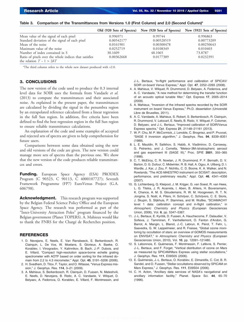
Table 3 lists several parameters that are used to make thecomparison between the two versions of the code. The valuesin the second column (for the 920 suited sets of spectra) are ofthe order of magnitude of the values in the third column (forthe whole 5921 sets of spectra) produced with v2.0. For thedataset used for the comparison, the new version producesmean transmittances closer to 1. The mean noise value isfive times smaller for the new code, remembering that the

calculated errors by the previous version of the code 1.0 withthe line shape and an order of magnitude lower than the newones are not part of the 920 sets of spectra used for comparison.The new set of data contains also more indices above theabsorption region. This means that transmittances are now ob-tained for higher altitudes. The mean noise value for the wholenew dataset is moreover a third smaller than the one calculatedfor the comparison set.

The T − 1 > 2δT comparison is larger for the new set ofspectra because the noise is larger in the old dataset whilethe transmittances for both old and new versions are very sim-ilar. This can explain the “anticorrelation” observed between thenoise and the success of the relation T − 1 > 2δT in the twofirst columns.

The version 2.0 of the code has been used to determinethe transmittances of 5921 sets of spectra over the 6232 totalsets of spectra, i.e., 95% of the sets of spectra are present inPSA level 3. The main reason why the remaining sets ofspectra could not be treated is that the Sun A region has anunsuitable shape (Fig. 5 is an example). In total, the newversion contains 735 sets of spectra that were not present inthe old version (among them, 271 sets of spectra before orbit2855.2, i.e., the last calculated one with the old version ofthe code).

Fig. 6. Transmittances calculated by (A) version 1.0 and (B) version2.0 for orbit 892.1 order 119 bin 1. The different spectra correspond-ing to different tangent altitudes are plotted on the same graph.

Fig. 7. Errors for orbit 1024.1, order 121 bin 1. (A) The old versionis on top, and (B) the new version below (the scale of δT is in 10−4 forthe old version and in 10−3 for the new one).

9280 Vol. 55, No. 32 / November 10 2016 / Applied Optics Research Article

3. CONCLUSIONS

The new version of the code used to produce the 0.3 internallevel data for SOIR uses the formula from Vandaele et al.(2013) to compute the transmittances and their associatednoise. As explained in the present paper, the transmittancesare calculated by dividing the signal in the penumbra regionby an extrapolated reference calculated from a linear regressionin the full Sun region. In addition, five criteria have beendefined to find the best regression region in the full Sun regionto ensure reliable transmittance calculations.

An explanation of the code and some examples of acceptedand rejected sets of spectra are given to help comprehension forfuture users.

Comparisons between some data obtained using the newand old versions of the code are given. The new version couldmanage more sets of spectra than the previous one. We showthat the new version of the code produces reliable transmittan-ces and errors.

Funding. European Space Agency (ESA) PRODEXProgram (C 90323, C 90113, C 4000107727); SeventhFramework Programme (FP7) EuroVenus Project (G.A.606798).

Acknowledgment. This research program was supportedby the Belgian Federal Science Policy Office and the EuropeanSpace Agency. The research was performed as part of the“Inter-University Attraction Poles” program financed by theBelgian government (Planet TOPERS). A. Mahieux would liketo thank the FNRS for the Chargé de Recherches position.

REFERENCES1. D. Nevejans, E. Neefs, E. Van Ransbeeck, S. Berkenbosch, R.

Clairquin, L. De Vos, W. Moelans, S. Glorieux, A. Baeke, O.Korablev, I. Vinogradov, Y. Kalinnikov, B. Bach, J.-P. Dubois, andE. Villard, “Compact high-resolution space-borne echelle gratingspectrometer with AOTF based on order sorting for the infrared do-main from 2.2 to 4.3 micrometer,” Appl. Opt. 45, 5191–5206 (2006).

2. H. Svedhem, D. Titov, F. Taylor, and O.Witasse, “Venus Express mis-sion,” J. Geophys. Res. 114, 3–21 (2009).

3. A. Mahieux, S. Berkenbosch, R. Clairquin, D. Fussen, N. Mateshvili,E. Neefs, D. Nevejans, B. Ristic, A. C. Vandaele, V. Wilquet, D.Belyaev, A. Fedorova, O. Korablev, E. Villard, F. Montmessin, and

J.-L. Bertaux, “In-flight performance and calibration of SPICAV/SOIR on-board Venus Express,” Appl. Opt. 47, 2252–2265 (2008).

4. A. Mahieux, V. Wilquet, R. Drummond, D. Belyaev, A. Federova, andA. C. Vandaele, “A new method for determining the transfer functionof an acousto optical tunable filter,” Opt. Express 17, 2005–2014(2009).

5. A. Mahieux, “Inversion of the infrared spectra recorded by the SOIRinstrument on board Venus Express,” Ph.D. dissertation (UniversitéLibre de Bruxelles, 2011).

6. A. C. Vandaele, A. Mahieux, S. Robert, S. Berkenbosch, R. Clairquin,R. Drummond, V. Letocart, E. Neefs, B. Ristic, V. Wilquet, F. Colomer,D. Belyaev, and J.-L. Bertaux, “Improved calibration of SOIR/VenusExpress spectra,” Opt. Express 21, 21148–21161 (2013).

7. W. P. Chu, M. P. McCormick, J. Lenoble, C. Brogniez, and P. Pruvost,“SAGE II inversion algorithm,” J. Geophys. Res. 94, 8339–8351(1989).

8. L. E. Mauldin, R. Salikhov, S. Habib, A. Vladimirov, D. Carraway,G. Petrenko, and J. Comella, “Meteor-3M-/stratospheric aerosoland gas experiment III (SAGE III),” Proc. SPIE 3501, 355–365(1998).

9. C. T. McElroy, C. R. Nowlan, J. R. Drummond, P. F. Bernath, D. V.Barton, D. G. Dufour, C. Midwinter, R. B. Hall, A. Ogyu, A. Ullberg, D. I.Wardle, J. Kar, J. Zou, F. Nichitiu, C. D. Boone, K. A. Walker, and N.Rowlands, “The ACE-MAESTRO instrument on SCISAT: description,performance, and preliminary results,” Appl. Opt. 46, 4341–4356(2007).

10. G. Lichtenberg, Q. Kleipool, J. M. Krijger, G. van Soest, R. van Hees,L. G. Tilstra, J. R. Acarreta, I. Aben, B. Ahlers, H. Bovensmann,K. Chance, A. M. S. Gloudemans, R. W. M. Hoogeveen, R. T. N.Jongma, S. Noël, A. Piters, H. Schrijver, C. Schrijvers, C. E. Sioris,J. Skupin, S. Slijkhuis, P. Stammes, and M. Wuttke, “SCIAMACHYlevel 1 data: calibration concept and in-flight calibration,” inAtmospheric Chemistry and Physics (European GeosciencesUnion, 2006), Vol. 6, pp. 5347–5367.

11. J.-L. Bertaux, E. Kyrölä, D. Fussen, A. Hauchecorne, F. Dalaudier, V.Sofieva, J. Tamminen, F. Vanhellemont, O. Fanton d’Andon, G.Barrot, A. Mangin, L. Blanot, J.-C. Lebrun, K. Pérot, T. Fehr, L.Saavedra, G. W. Leppelmeier, and R. Fraisse, “Global ozone moni-toring by occultation of stars: an overview of GOMOS measurementson ENVISAT,” in Atmospheric Chemistry and Physics (EuropeanGeosciences Union, 2010), Vol. 10, pp. 12091–121480.

12. S. Lebonnois, E. Quémerais, F. Montmessin, F. Lefèvre, S. Perrier,J.-L. Bertaux, and F. Forget, “Vertical distribution of ozone on Marsas measured by SPICAM/Mars Express using stellar occultations,”J. Geophys. Res. 111, E09S05 (2006).

13. E. Quémerais, J.-L. Bertaux, O. Korablev, E. Dimarellis, C. Cot, B. R.Sandel, and D. Fussen, “Stellar occultations observed by SPICAM onMars Express,” J. Geophys. Res. 111, E09S04 (2006).

14. C. H. Acton, “Ancillary data services of NASA’s navigational andancillary information facility,” Planet. Space Sci. 44, 65–70(1996).

Table 3. Comparison of the Transmittances from Versions 1.0 (First Column) and 2.0 (Second Column)a

Old (920 Sets of Spectra) New (920 Sets of Spectra) New (5921 Sets of Spectra)

Mean value of the signal of each pixel 0.996971 0.99744 0.996863Standard deviation of the signal of each pixel 0.00542177 0.00528519 0.00773209Mean of the noise 0.0161901 0.00300478 0.00250643Maximum value of the noise 0.0252719 0.0108349 0.010403Number of index contained in S 30.1609 48.1065 73.8787Ratio of pixels over the whole indices that satisfiesthe relation T − 1 > 2δT

0.00362668 0.0177389 0.0232391

aThe third column refers to the whole new dataset produced with v2.0.

Research Article Vol. 55, No. 32 / November 10 2016 / Applied Optics 9281