Representing 3D models for alignment and recognition
183
HAL Id: tel-01160300 https://tel.archives-ouvertes.fr/tel-01160300v2 Submitted on 11 Apr 2018 HAL is a multi-disciplinary open access archive for the deposit and dissemination of sci- entific research documents, whether they are pub- lished or not. The documents may come from teaching and research institutions in France or abroad, or from public or private research centers. L’archive ouverte pluridisciplinaire HAL, est destinée au dépôt et à la diffusion de documents scientifiques de niveau recherche, publiés ou non, émanant des établissements d’enseignement et de recherche français ou étrangers, des laboratoires publics ou privés. Representing 3D models for alignment and recognition Mathieu Aubry To cite this version: Mathieu Aubry. Representing 3D models for alignment and recognition. Computer Vision and Pattern Recognition [cs.CV]. Ecole normale supérieure - ENS PARIS, 2015. English. NNT : 2015ENSU0006. tel-01160300v2
Transcript of Representing 3D models for alignment and recognition
HAL Id: tel-01160300https://tel.archives-ouvertes.fr/tel-01160300v2
Submitted on 11 Apr 2018
HAL is a multi-disciplinary open accessarchive for the deposit and dissemination of sci-entific research documents, whether they are pub-lished or not. The documents may come fromteaching and research institutions in France orabroad, or from public or private research centers.
L’archive ouverte pluridisciplinaire HAL, estdestinée au dépôt et à la diffusion de documentsscientifiques de niveau recherche, publiés ou non,émanant des établissements d’enseignement et derecherche français ou étrangers, des laboratoirespublics ou privés.
Representing 3D models for alignment and recognitionMathieu Aubry
To cite this version:Mathieu Aubry. Representing 3D models for alignment and recognition. Computer Vision and PatternRecognition [cs.CV]. Ecole normale supérieure - ENS PARIS, 2015. English. �NNT : 2015ENSU0006�.�tel-01160300v2�

ED 386 : Sciences mathématiques de Paris Centre
Informatique
Mathieu Aubry
8 mai 2015
Representing 3D models for alignment and recognition
équipe WILLOW (CNRS/ENS/INRIA UMR 8548)
Daniel Cremers (TU Munich)
Josef Sivic (INRIA-ENS)
Jean Ponce (ENS) Léonidas Guibas (Stanford)
Bryan Russell (Adobe) Martial Hebert (CMU)

2
Abstract
Thanks to the success of 3D reconstruction algorithms and the devel-
opment of online tools for computer-aided design (CAD) the number
of publicly available 3D models has grown significantly in recent years,
and will continue to do so. This thesis investigates representations of
3D models for 3D shape matching, instance-level 2D-3D alignment, and
category-level 2D-3D recognition.
The geometry of a 3D shape can be represented almost completely by
the eigen-functions and eigen-values of the Laplace-Beltrami operator on
the shape. We use this mathematically elegant representation to char-
acterize points on the shape, with a new notion of scale. This 3D point
signature can be interpreted in the framework of quantum mechanics and
we call it the Wave Kernel Signature (WKS). We show that it has ad-
vantages with respect to the previous state-of-the-art shape descriptors,
and can be used for 3D shape matching, segmentation and recognition.
— M. Aubry : Representing 3D models for alignment and recognition —

3
A key element for understanding images is the ability to align an object
depicted in an image to its given 3D model. We tackle this instance
level 2D-3D alignment problem for arbitrary 2D depictions including
drawings, paintings, and historical photographs. This is a tremendously
difficult task as the appearance and scene structure in the 2D depic-
tions can be very different from the appearance and geometry of the
3D model, e.g., due to the specific rendering style, drawing error, age,
lighting or change of seasons. We represent the 3D model of an entire
architectural site by a set of visual parts learned from rendered views of
the site. We then develop a procedure to match those scene parts that
we call 3D discriminative visual elements to the 2D depiction of the ar-
chitectural site. We validate our method on a newly collected dataset
of non-photographic and historical depictions of three architectural sites.
We extend this approach to describe not only a single architectural site
but an entire object category, represented by a large collection of 3D
CAD models. We develop a category-level 2D-3D alignment method
that not only detects objects in cluttered images but also identifies their
approximate style and viewpoint. We evaluate our approach both qual-
— M. Aubry : Representing 3D models for alignment and recognition —

4
itatively and quantitatively on a subset of the challenging Pascal VOC
2012 images of the “chair” category using a reference library of 1394
CAD models downloaded from the Internet.
— M. Aubry : Representing 3D models for alignment and recognition —

5
Acknowledgments
I want first to thank all the people I will never forget but cannot list whoinspired, supported or advised me, shared coffees, drinks or thoughtswith me, and made those last years as rich as they were. This thesiswould not be the same without them.The people I will individually thank are those who made me discoverComputer Vision.
My interest in Vision began with the outstanding Cognitive Science lec-ture of Jean Petitot who was also the one who advised me to follow theMVA master. My thanks also go to Renaud Keriven who welcomed mein the Imagine Group of the ENPC, and sent me to discover the Com-puter Vision group of Daniel Cremers in Munich and Computer Graphicsat Adobe in Boston.
In Munich Bastian Goldluecke kindly helped me discovering energy min-imization and writing my first paper. I also had the chance to meet Ul-rich Schlickewei who believed in the idea WKS from the very beginning,helped me to develop it and without whom it would not be what it is.
I am very grateful to Sylvain Paris for his warm welcome in Boston,his guidance and his encouragements to discover photography and Com-puter Graphics. My thanks also go to Fredo Durand who allowed me todiscover MIT Graphics group and whose rigor will remain an inspiration.
I had the chance to have two outstanding PhD advisors. Daniel Cre-mers built in Munich an impressive, friendly and welcoming group andI am especially grateful to him for the confidence he showed and gaveme. Josef Sivic shared with me his passion for research and Vision. Hisvision, the support and guidance he gave me were invaluable. Thanksto him I also had the chance to meet and work with Bryan Russell andAlyosha Efros. Finally, I am deeply indebted to Josef for correcting andproofreading this thesis.
— M. Aubry : Representing 3D models for alignment and recognition —

6
Last but not least, I am grateful to Leonidas Guibas and Martial Hebertwho agreed to be the “rapporteurs” of this thesis and to Jean Ponce whoagreed to be my thesis committee director.
I cannot finish without mentioning my family, whose support, under-standing and influence are beyond words, in particular my brothers,Thomas and Thibaut, my parents, Gabriel and Beatrice, and my grand-mother Francoise.
— M. Aubry : Representing 3D models for alignment and recognition —

CONTENTS 7
Contents
1 Introduction 11
1.1 Goals . . . . . . . . . . . . . . . . . . . . . . . . . . . . . . . . . . . . . 11
1.2 Motivation . . . . . . . . . . . . . . . . . . . . . . . . . . . . . . . . . . 13
1.3 Challenges . . . . . . . . . . . . . . . . . . . . . . . . . . . . . . . . . . 14
1.3.1 3D local descriptors . . . . . . . . . . . . . . . . . . . . . . . . . 15
1.3.2 Instance-level 2D-3D alignment . . . . . . . . . . . . . . . . . . 16
1.3.3 Category-level 2D-3D object recognition . . . . . . . . . . . . . 18
1.4 Contributions . . . . . . . . . . . . . . . . . . . . . . . . . . . . . . . . 20
1.4.1 Wave Kernel Signature . . . . . . . . . . . . . . . . . . . . . . . 20
1.4.2 3D discriminative visual elements . . . . . . . . . . . . . . . . . 21
1.5 Thesis outline . . . . . . . . . . . . . . . . . . . . . . . . . . . . . . . . 21
1.6 Publications . . . . . . . . . . . . . . . . . . . . . . . . . . . . . . . . . 23
2 Background 25
2.1 3D shape analysis . . . . . . . . . . . . . . . . . . . . . . . . . . . . . . 25
2.1.1 From the ideal shapes to discrete 3D models . . . . . . . . . . . 26
2.1.2 3D point descriptors . . . . . . . . . . . . . . . . . . . . . . . . 28
2.1.3 3D shape alignment methods . . . . . . . . . . . . . . . . . . . 33
2.2 Instance-level 2D-3D alignment . . . . . . . . . . . . . . . . . . . . . . 36
— M. Aubry : Representing 3D models for alignment and recognition —

CONTENTS 8
2.2.1 Contour-based methods . . . . . . . . . . . . . . . . . . . . . . 36
2.2.2 Local features for alignment . . . . . . . . . . . . . . . . . . . . 40
2.2.3 Global features for alignment . . . . . . . . . . . . . . . . . . . 46
2.2.4 Relationship to our method . . . . . . . . . . . . . . . . . . . . 47
2.3 Category-level 2D-3D alignment . . . . . . . . . . . . . . . . . . . . . . 47
2.3.1 2D methods . . . . . . . . . . . . . . . . . . . . . . . . . . . . . 48
2.3.2 3D methods . . . . . . . . . . . . . . . . . . . . . . . . . . . . . 52
2.3.3 Relationship to our method . . . . . . . . . . . . . . . . . . . . 53
3 Wave Kernel Signature 55
3.1 Introduction . . . . . . . . . . . . . . . . . . . . . . . . . . . . . . . . . 55
3.1.1 Motivation . . . . . . . . . . . . . . . . . . . . . . . . . . . . . . 56
3.1.2 From Quantum Mechanics to shape analysis . . . . . . . . . . . 57
3.1.3 Spectral Methods for shape analysis . . . . . . . . . . . . . . . . 59
3.2 The Wave Kernel Signature . . . . . . . . . . . . . . . . . . . . . . . . 65
3.2.1 From heat diffusion to Quantum Mechanics . . . . . . . . . . . 65
3.2.2 Schrodinger equation on a surface . . . . . . . . . . . . . . . . . 67
3.2.3 A spectral signature for shapes . . . . . . . . . . . . . . . . . . 68
3.2.4 Global vs. local WKS . . . . . . . . . . . . . . . . . . . . . . . 70
3.3 Mathematical Analysis of the WKS . . . . . . . . . . . . . . . . . . . . 71
3.3.1 Stability analysis . . . . . . . . . . . . . . . . . . . . . . . . . . 71
3.3.2 Spectral analysis . . . . . . . . . . . . . . . . . . . . . . . . . . 75
3.3.3 Invariance and discrimination . . . . . . . . . . . . . . . . . . . 76
3.4 Experimental Results . . . . . . . . . . . . . . . . . . . . . . . . . . . . 77
3.4.1 Qualitative analysis . . . . . . . . . . . . . . . . . . . . . . . . . 77
— M. Aubry : Representing 3D models for alignment and recognition —
CONTENTS 9
3.4.2 Quantitative evaluation . . . . . . . . . . . . . . . . . . . . . . . 81
3.5 Applications . . . . . . . . . . . . . . . . . . . . . . . . . . . . . . . . . 87
3.6 Conclusion . . . . . . . . . . . . . . . . . . . . . . . . . . . . . . . . . . 90
4 Painting-to-3D Alignment 91
4.1 Introduction . . . . . . . . . . . . . . . . . . . . . . . . . . . . . . . . . 91
4.1.1 Motivation . . . . . . . . . . . . . . . . . . . . . . . . . . . . . . 93
4.1.2 From locally invariant to discriminatively trained features . . . 93
4.1.3 Overview . . . . . . . . . . . . . . . . . . . . . . . . . . . . . . 94
4.2 3D discriminative visual elements . . . . . . . . . . . . . . . . . . . . . 96
4.2.1 Learning 3D discriminative visual elements . . . . . . . . . . . . 97
4.2.2 Matching as classification . . . . . . . . . . . . . . . . . . . . . 98
4.3 Discriminative visual elements for painting-to-3D alignment . . . . . . 100
4.3.1 View selection and representation . . . . . . . . . . . . . . . . . 100
4.3.2 Least squares model for visual element selection and matching . 102
4.3.3 Calibrated discriminative matching . . . . . . . . . . . . . . . . 107
4.3.4 Filtering elements unstable across viewpoint . . . . . . . . . . . 108
4.3.5 Robust matching . . . . . . . . . . . . . . . . . . . . . . . . . . 111
4.3.6 Recovering viewpoint . . . . . . . . . . . . . . . . . . . . . . . . 111
4.3.7 Summary . . . . . . . . . . . . . . . . . . . . . . . . . . . . . . 112
4.4 Results and validation . . . . . . . . . . . . . . . . . . . . . . . . . . . 113
4.4.1 Dataset for painting-to-3D alignment . . . . . . . . . . . . . . . 113
4.4.2 Qualitative results . . . . . . . . . . . . . . . . . . . . . . . . . 114
4.4.3 Quantitative evaluation . . . . . . . . . . . . . . . . . . . . . . . 117
4.4.4 Algorithm analysis . . . . . . . . . . . . . . . . . . . . . . . . . 124
— M. Aubry : Representing 3D models for alignment and recognition —

CONTENTS 10
4.5 Conclusion . . . . . . . . . . . . . . . . . . . . . . . . . . . . . . . . . . 129
5 Seeing 3D Chairs 131
5.1 Introduction . . . . . . . . . . . . . . . . . . . . . . . . . . . . . . . . . 131
5.1.1 Motivation . . . . . . . . . . . . . . . . . . . . . . . . . . . . . . 133
5.1.2 From instance-level to category-level alignment . . . . . . . . . 134
5.1.3 Approach Overview . . . . . . . . . . . . . . . . . . . . . . . . . 135
5.2 Discriminative visual elements for category-level 3D-2D alignment . . . 136
5.2.1 Representing a 3D shape collection . . . . . . . . . . . . . . . . 136
5.2.2 Calibrating visual element detectors . . . . . . . . . . . . . . . . 140
5.2.3 Matching spatial configurations of visual elements . . . . . . . . 141
5.3 Experiments and results . . . . . . . . . . . . . . . . . . . . . . . . . . 143
5.3.1 Large dataset of 3D chairs . . . . . . . . . . . . . . . . . . . . . 145
5.3.2 Qualitative results . . . . . . . . . . . . . . . . . . . . . . . . . 145
5.3.3 Quantitative evaluation . . . . . . . . . . . . . . . . . . . . . . . 147
5.3.4 Algorithm analysis . . . . . . . . . . . . . . . . . . . . . . . . . 150
5.4 Conclusion . . . . . . . . . . . . . . . . . . . . . . . . . . . . . . . . . . 154
6 Discussion 156
6.1 Contributions . . . . . . . . . . . . . . . . . . . . . . . . . . . . . . . . 156
6.2 Future work . . . . . . . . . . . . . . . . . . . . . . . . . . . . . . . . . 157
6.2.1 Anisotropic Laplace-Beltrami operators . . . . . . . . . . . . . . 157
6.2.2 Object compositing . . . . . . . . . . . . . . . . . . . . . . . . . 158
6.2.3 Use of 3D shape collection analysis . . . . . . . . . . . . . . . . 159
6.2.4 Synthetic data for deep convolutional network training . . . . . 159
6.2.5 Exemplar based approach with CNN features . . . . . . . . . . 159
— M. Aubry : Representing 3D models for alignment and recognition —

11
Chapter 1
Introduction
1.1 Goals
The goal of this thesis is to develop representations of 3D models for (i) alignment with
other 3D models, (ii) alignment with an image containing the same object instance and
(iii) alignment with an image containing an object from the same category. Those three
tasks are illustrated in figure 1.1. What is a “good” representation will depend on the
task :
• Matching, segmentation and recognition of 3D shapes: Shape matching
aims at computing correspondences between two similar 3D shapes. Shape seg-
mentation attempts to partition the shape into a set of meaningful regions by
analyzing the single shape or a collection of 3D shapes. Finally, shape recogni-
tion typically classifies a given shape into categories defined by examples of other
shapes. The work presented in chapter 3 aims at improving the 3D point de-
scriptors that are used for those tasks by modeling and optimizing the descriptor
variability. An example of shape matching is shown on figure 1.1a.
— M. Aubry : Representing 3D models for alignment and recognition —

Section 1.1: Goals 12
(a) Matching between two 3D shapes using our Wave Kernel Signature.
(b) Examples of non-photographic depictions of Notre Dame in Paris correctly alignedto its 3D model (shown in the top left inset) and visualized in Google Earth [56]
(c) Approximate models correctly recovered by our algorithm and overlapped with theinput image (left) in their recovered viewpoint (right).
Figure 1.1: The three different 3D model alignment tasks addressed in this thesis.
— M. Aubry : Representing 3D models for alignment and recognition —

Section 1.2: Motivation 13
• Instance-level 2D-3D alignment across depiction style: while computer
vision has mainly focused on analyzing photographs, we aim at understanding
historical and non-photographic imagery. Given the 3D model of an architectural
site and its 2D depiction, we wish to recover the viewpoint of the image with
respect to the 3D model. To apply this idea on a large scale, our goal is to
develop an automatic method that is robust to the style variations, to the errors
in the depictions and to the variable quality of the 3D model. Examples of
paintings aligned by our algorithm with a 3D model of Notre-Dame in Paris are
shown on figure 1.1b.
• Object category-level recognition by 2D-3D alignment: we want to go
beyond instance-level alignment, which requires knowing in advance the 3D mod-
els of the object instances present in the image, and develop category-level 2D-3D
alignment. We assume that the object categories are represented by large collec-
tions of 3D CAD models. Our goal is to take as input an unseen image and to
output not only the categories of the objects that are present but also approxi-
mate 3D models, correctly aligned with the input depiction, as shown in figure
1.1c.
1.2 Motivation
Automatic, high quality, large scale 3D reconstructions are one of the major successes
of computer vision. It is now possible to easily scan an object with a smart phone
[104, 172], capture a living room with a Kinect [91, 131, 159], or visit a virtual city on
Google Earth [56]. Computer-aided design has also evolved to the point that public or
commercial libraries of millions of 3D models of objects are available [157, 175]. This
— M. Aubry : Representing 3D models for alignment and recognition —

Section 1.3: Challenges 14
growing amount of data, of which some examples are shown in figure 1.2, requires new
tools but also is an opportunity to develop new applications. Example applications
include:
• Browsing and parametrization of large shape collections. Creating a new
3D model requires time and expert knowledge. Instead of always creating new
models, the designer could browse, search, and manipulate in an intuitive way
existing 3D models in the collection.
• Browsing historical data. Imagine a computer could automatically recover the
viewpoint of all existing historical imagery. This could change the way archivists,
architects or historians access and browse archives of historical images. The users
could browse the images intuitively and to compare depictions from similar places
at different times.
• Smart image editing. Imagine a computer could identify objects in an input
2D image and automatically recover their 3D models. It would be possible to
use the recovered 3D model to edit the image by manipulating objects in 3D.
Currently, this editing requires manual annotation [100].
• Robotic manipulation. For a robot to manipulate an object, it needs to know
not only in which direction the object is, but also to have access to its 3D model
including, for example, unseen parts.
1.3 Challenges
While there are several exciting applications for 3D alignment, finding good represen-
tations and matching algorithms is very difficult.
— M. Aubry : Representing 3D models for alignment and recognition —

Section 1.3: Challenges 15
(a) Interactive reconstruction with acell phone [172]
(b) Reconstruction of a room withKinect fusion [91]
(c) High-resolution reconstructionby Acute3D [5]
(d) Berkeley campus on GoogleEarth [56]
(e) Search for 3D models of chairs on Trimble 3D Warehouse [175]
Figure 1.2: 3D models are becoming common and easy to acquire.
1.3.1 3D local descriptors
Defining purely geometric descriptors for 3D shapes is a difficult and open problem.
An good descriptor for a point on a 3D shape would:
• be discriminative to distinguish different points on the shape as well as different
shapes from each other.
• be robust to perturbations such as near-isometric deformations, noise or topo-
— M. Aubry : Representing 3D models for alignment and recognition —

Section 1.3: Challenges 16
(a) Reference shape (b) Noise (c) Local dilatation (d) Near-isometric
Figure 1.3: Challenges of 3D shape alignment. Examples of shape perturbations fromthe TOSCA dataset [50].
logical changes. Examples of such perturbations are shown in figure 1.3. This is
needed for or example to match two models of a person in different poses or to
align models of different quadrupeds.
• include informations from all scales of the shape to allow recognition and match-
ing of parts of the shape, for example to recognize a handle within a 3D model
of a complete door.
Those characteristics are hard to achieve and are often conflicting. We focus particu-
larly on the trade-off between robustness and discriminative power, while developing a
new intuition about scale.
1.3.2 Instance-level 2D-3D alignment
Viewpoint, illumination and occlusion. First, the space of possible viewpoints of
the same 3D model is huge, especially for a full architectural site, and the appearance
of the 3D model can change significantly with the viewpoint as shown in figure 1.4a.
Second, the illumination conditions, for example related to the season and the time
of the day also change significantly the appearance of the scene as shown in figure
1.4b and 1.4c. Third, the appearance of the 3D model itself is highly specific, ranging
from simplified CAD models to highly detailed models obtained from recent multi-view
— M. Aubry : Representing 3D models for alignment and recognition —

Section 1.3: Challenges 17
(a) Viewpoint changes
(b) Illumination changes
(c) Season changes
(d) Model specific appearance
(e) Clutter and occlusion
(f) Historical and non-photographic imagery
Figure 1.4: Challenges of 2D-3D instance alignment.
— M. Aubry : Representing 3D models for alignment and recognition —

Section 1.3: Challenges 18
Figure 1.5: Matching local features, such as SIFT [121] often works well for two sim-ilar photographs (left), but fails between two very different images such as a photographand a watercolor (right). This figure shows the most confident SIFT matches betweenthe top image and the two bottom images in terms of the first to second nearest neighborratio [121].
stereo algorithms, as can be seen in figure 1.4d. Finally, in many cases, occlusions and
clutter change the appearance of an image as shown figure 1.4e.
Depiction style and drawing errors. Non-realistic depictions such as paintings,
drawings and engravings are even harder to work with. They have very particular
depiction style and often (sometime intentional) drawing errors. In some cases, the
appearance of the place may have changed over time, because of construction or aging.
Examples of such effects are shown in figure 1.4f. For these reasons, local descriptors,
such as SIFT [121], traditionally used for instance-level alignment, often fail for non-
realistic depictions as shown in figure 1.5.
1.3.3 Category-level 2D-3D object recognition
The difficulties discussed above for instance-level alignment also apply to category-
level alignment. An example can be seen in figure 1.6 where recognizing objects,
such as chairs, is difficult because of the occlusions, shadows, clutter and the different
— M. Aubry : Representing 3D models for alignment and recognition —

Section 1.3: Challenges 19
Figure 1.6: Aligning 3D models to objects, such as chairs in this image is difficultbecause of occlusion, clutter, the different viewpoints and illumination effects. Notethat this image was computer generated.
Figure 1.7: Intra-class variation is one of the main challenges of category-level recog-nition. This figure shows a small set of chairs with different appearance, topology andparts.
viewpoints.
Intra-class variation. To recognize not only a given instance but any instance from
a given object category, we must also deal with the intra-class variation. The different
instances belonging to the same category can have different textures, more or less parts
parts or even a completely different topology, as shown in figure 1.7 for the “chair”
— M. Aubry : Representing 3D models for alignment and recognition —

Section 1.4: Contributions 20
category.
1.4 Contributions
This section presents the two main contributions of this thesis. More details about the
technical contributions are given in section 6.1.
1.4.1 Wave Kernel Signature
One of the basic tasks in shape processing is to establish correspondences between two
shapes (cf. figure 1.1a). This can be achieved by associating to each point of the two
shapes a descriptor with two (conflicting) characteristics: being (i) discriminative and
(ii) invariant to deformations. In chapter 3, we analyze the influence of variations in
the metric on the eigen-values of the Laplace-Beltrami operator. This leads to the
definition of a descriptor that provides an optimal trade-off between discriminativeness
and invariance. We show that this descriptor, that we call the Wave Kernel Signature
(WKS), can be naturally interpreted in the framework of Quantum Mechanics as the
average probability of finding a particle of a given energy distribution freely diffusing
on the shape at the specific point it describes. We compare this descriptor to the Heat
Kernel Signature (HKS), which has a similar formulation and show the difference in
the notion of scale they imply. We evaluate our descriptor on the standard SHREC
2010 benchmark [33] and show that for some tasks the WKS improves over the HKS,
which is the state-of-the-art shape descriptor. We also show that the WKS can be used
for shape segmentation and retrieval.
— M. Aubry : Representing 3D models for alignment and recognition —

Section 1.5: Thesis outline 21
1.4.2 3D discriminative visual elements
We bring to 3D the notion of discriminative visual elements and introduce 3D discrim-
inative visual elements to represent 3D models for 2D-3D alignment and recognition.
These are visual parts extracted from rendered views of a 3D model and are associated
to a calibrated 2D sliding window detector and a 3D location, orientation and scale
on the model. The extracted parts summarize the 3D model in a way that is suitable
for part-based matching to 2D depictions. The two most important technical points
in the definition of the discriminative visual elements are: (i) their selection, based on
a discriminative cost function and (ii) the definition and calibration of the associated
detector. We use the visual elements to address two challenges. In chapter 4 we use 3D
discriminative visual elements to solve a difficult instance alignment problem: aligning
non-photographic depictions to 3D models of architectural sites. In chapter 5 we show
that the extracted elements can also be used to describe object categories defined by
collections of 3D models. In detail, we show that 3D discriminative visual elements can
be used to to detect and recognize a new instance of an object category in real world
photographs, and to provide an approximate viewpoint and 3D model of the detected
instance.
1.5 Thesis outline
In chapter 2 we review methods in 3D shape analysis, instance-level alignment and
category-level recognition that are most related to this thesis. In detail, we give an
overview of 3D shape representation and alignment methods, 2D-3D contour-based and
local feature-based alignment, and category-level recognition in images using 2D and
3D methods.
— M. Aubry : Representing 3D models for alignment and recognition —
Section 1.5: Thesis outline 22
In chapter 3 we introduce a novel geometric descriptor for 3D shapes, the Wave Kernel
Signature and explain how it relates to existing descriptors. In particular, we develop a
model of shape perturbations that shows that it achieves an optimal trade-off between
robustness and discriminability and we present the notion of scale separation to which
it is associated. We experimentally compare its performance to other descriptors, ex-
plain why it improves on current state-of-the-art results and show that it can be used
for shape matching, segmentation and recognition.
In chapter 4 we present and analyze a new method for registering non-photographic de-
pictions of an architectural site with its 3D model. We introduce a new representation
of the 3D model formed by visually informative parts that are learned from rendered
views of the model, together with a robust matching method to detect the parts in
2D depictions despite changes in the depiction style. We analyze both contributions
separately and compare our full method with different alternatives that we designed
based on state-of-the-art algorithms. For this evaluation we introduce a new dataset
of non-photographic and historical depictions and run an extensive user study.
Finally, in chapter 5 we present a method to perform category-level object recognition
by 2D-3D alignment. The shape representation introduced in chapter 4 is extended
to represent not only a single 3D model but an entire object category. In particular,
we introduce a new efficient calibration of part detector scores based only on negative
data. We evaluate our method on the standard PASCAL VOC dataset for object
category detection. Our method provides more information about an image content
than standard recognition methods since it goes beyond predicting a name for an object
or its approximate bounding-box, but also provides an approximate 3D model aligned
— M. Aubry : Representing 3D models for alignment and recognition —

Section 1.6: Publications 23
with the input image.
1.6 Publications
The idea of the Wave Kernel signature presented in chapter 3 was published in 2011
in an ECCV workshop, 4DMOD [21], and the applications of this descriptor to seg-
mentation and recognition the same year in DAGM/GCPR [20]. The first work [21]
has already been cited more than 90 times and an extended version is in submission
to PAMI. The painting-to-3d alignment work presented in chapter 4 was released as a
technical report in 2013, published in TOG and presented at Siggraph in 2014 [17]. A
shorter version was published as an invited paper in RFIA 2014 [19] and it lead to an
invited presentation in the “Registration of Very Large Images” workshop at CVPR
2014. An extension to geo-localization is going to appear as a book chapter [18]. Fi-
nally, the work on object category recognition from 3D shape collections presented in
chapter 5 was published at CVPR 2014 [14].
The code corresponding to those projects and the publications are publicly available
[2, 3, 4].
I have also published several papers that go beyond the scope of this thesis. The work
of my Master degree on the relationship between dense camera calibration and bundle
adjustment was published in ICCV 2011 [13] and was included by Bastian Goldlucke
in a paper published in IJCV 2014 [77]. The work I did during an internship at Adobe
on detail manipulation and style transfer was released as a technical report in 2011 [16]
and published in TOG and presented at Siggraph in 2014 [15]. Finally, an idea about
the use of anisotropy for shape analysis, briefly presented in 6.2.1 was developed by
— M. Aubry : Representing 3D models for alignment and recognition —

Section 1.6: Publications 24
Mathieu Andreux and published in NORDIA, an ECCV workshop, in 2014 [10].
— M. Aubry : Representing 3D models for alignment and recognition —

25
Chapter 2
Background
This thesis builds on ideas from what have traditionally been separate sub-fields of
computer vision, namely 3D shape analysis, instance-level alignment and category-level
recognition in images. In this chapter, we give an overview of the classical methods that
are most relevant to this dissertation. Each following chapter of this thesis contains
more information about the novelty of the described method.
2.1 3D shape analysis
In this section, we will explain how the work presented in chapter 3 relates to the more
general problematic of 3D shape analysis and especially shape alignment methods. We
will first explain how 3D shapes can be represented in computers, then present the
main local descriptors that have been designed to describe these shapes, and finally
summarize the different competing approaches for shape alignment.
— M. Aubry : Representing 3D models for alignment and recognition —

Section 2.1: 3D shape analysis 26
2.1.1 From the ideal shapes to discrete 3D models
The first question that arises when working with shapes is: how to model them? We
have an intuitive notion of what the shape of an object is, but it is not straightforward
to formalize. When working with a computer it is also necessary to define a discrete
version of this intuition to represent the shape by a (digital) 3D model. In this section,
we present some of the main competing shape representations. ace from a discrete
point set), but their discussion is out of the scoop of this thesis.
2.1.1.1 Volumetric representation
One possible way to think about a shape is as a volume in the 3D space. The natural
way to define a discrete representation based on this intuition is to discretize the space
in a regular grid of voxels, and for each voxel to store if the central point is inside
or outside the volume [60]. The problem with this representation is that it is very
expensive in terms of memory consumption. The required memory is cubic with respect
to the resolution of the 3D model: to represent a shape in a cube of 1000x1000x1000
voxels, it is necessary to store one billion numbers. However, at the cost of a less
intuitive representation, the same volume can be represented more efficiently using
octrees [92].
This representation is often used in practice because several optimization algorithms
are naturally formulated in the voxel space. This is in particular the case for some
dense 3D reconstruction methods, of which an overview is available in [155]. The main
reason is that by relaxing the values associated to each voxel to [0; 1] instead of {0, 1}
it is often possible to formulate the problem as convex optimization that can be solved
efficiently. This relaxation also makes topology changes straightforward to handle.
— M. Aubry : Representing 3D models for alignment and recognition —

Section 2.1: 3D shape analysis 27
2.1.1.2 Point Clouds
Opposite to the intuition that a shape is a volume, used in dense representations, is
the idea that a shape is a collection of the points on its surface. Based on this idea,
a discrete representation of the shape can be computed by sampling a finite set of 3D
points on this surface. This set of points is sometimes augmented by the collection
of normals to the surface at each point. This is the natural representation when 3D
measurements are provided by a laser scans, which provide the position of a sparse set
of points, and also for many feature based 3D reconstruction algorithms (e.g. [70, 6])
which outputs are a set of points on the object surface. The main limitations of this
representation are that: (i) it depends on the sampling of the points and (ii) it does
not provide the surface of the object. For this reasons point clouds are often meshed.
2.1.1.3 Meshes
Meshes and, in particular, triangular meshes are probably today the most common
representation of shapes. Rather than specifying for each 3D point if it is inside or
outside the shape, or to simply list a set of points on the surface, a mesh represents the
shape by an approximation of its surface, which is often modeled as a 2-dimensional
manifold in R3. Concretely, a mesh is a set of vertices (3D points) and faces (sets of
coplanar vertices). Texture can be associated to a mesh by providing a color for each
vertex, or by mapping each face to an image. Models reconstructed automatically from
multiple images typically have one color per vertex, while models designed manually
typically associate an image to each face.
Most of the work presented in this thesis has been done with 3D shapes represented as
meshes, but could easily be adapted to use point clouds or volumetric representations.
— M. Aubry : Representing 3D models for alignment and recognition —

Section 2.1: 3D shape analysis 28
2.1.2 3D point descriptors
None of the shape representations described in section 2.1 is invariant to translation,
rotation or scaling. Given a point on a shape it is very difficult to match it, for example
in a rotated version of the same shape. For this reason local shape descriptors invariant
to rigid transformations have been developed. They can be understood as embeddings
of the shape in another space, potentially high dimensional. To cope with non-rigid
transformations, more elaborate descriptors have been designed to be robust to limited
non-isometric deformations.
In this thesis, we focus on the use of point signatures for matching and alignment, but
they can have different applications. In fact, the very idea of using a point signature
for 3D shapes has been introduced in [43] to use putative matches for recognition. An
alternative way to perform recognition with local features is to accumulate them into
global shape descriptor [12, 34, 71, 135]. Local descriptors have also been used for
shape segmentation [20, 145, 148]. Indeed a simple clustering such as K-means can be
meaningful in the descriptors space.
The main local shape descriptors can be separated in two categories. We first introduce
descriptors that accumulate local information about the shape in an histogram, and
then present spectral descriptors which utilize the eigen-decomposition of a differential
operator on the shape.
2.1.2.1 Descriptors based on local histograms
Those descriptors were developed first, following the success of similar methods in 2D
image analysis (see sections 2.2.2 and 2.3.1.2).
— M. Aubry : Representing 3D models for alignment and recognition —
Section 2.1: 3D shape analysis 29
Figure 2.1: Spin Image [94] defines a local image for each point of a shape based oncylindric coordinates. Figure from [94]
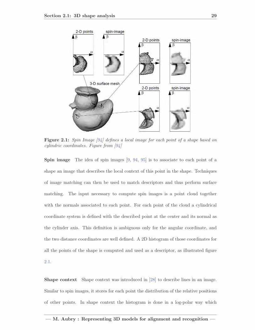
Spin image The idea of spin images [9, 94, 95] is to associate to each point of a
shape an image that describes the local context of this point in the shape. Techniques
of image matching can then be used to match descriptors and thus perform surface
matching. The input necessary to compute spin images is a point cloud together
with the normals associated to each point. For each point of the cloud a cylindrical
coordinate system is defined with the described point at the center and its normal as
the cylinder axis. This definition is ambiguous only for the angular coordinate, and
the two distance coordinates are well defined. A 2D histogram of those coordinates for
all the points of the shape is computed and used as a descriptor, as illustrated figure
2.1.
Shape context Shape context was introduced in [28] to describe lines in an image.
Similar to spin images, it stores for each point the distribution of the relative positions
of other points. In shape context the histogram is done in a log-polar way which
— M. Aubry : Representing 3D models for alignment and recognition —

Section 2.1: 3D shape analysis 30
(a) Original shape-context for 1D surfaces.Figure from [28]
(b) Shape context for 2D surfaces usinggeodesic distances. Figure from [103]
Figure 2.2: Shape context accumulates information in a log-polar way.
presents several advantages, including giving more importance to close-by points and
transforming rotations and scaling of the shape into a translation of the descriptor.
This is visualized figure 2.2a. The original article [28] also shows 3D object recognition
results using shape context on a set of views of the 3D model. The idea of shape context
was extended in a more principled way to shapes in 3D by [103, 106], as illustrated in
figure 2.2b.
Shape HOG: The idea of shape HOGs [183] is similar to shape context in the sense
that it computes histograms in log-polar coordinates, but it aims at describing a texture
on a shape rather than the shape itself. As a consequence, it stores histograms of the
dominant gradient orientations of the projected texture for each bin instead of the
density of points.
— M. Aubry : Representing 3D models for alignment and recognition —

Section 2.1: 3D shape analysis 31
Figure 2.3: The eigen-functions of the Laplace-Beltrami operator on a shape corre-spond to its vibration modes. The vibration modes are closely related to the shape, asvisualized here for 553, 731 and 1174Hz [66].
2.1.2.2 Spectral signatures
In most cases, one can recover all the intrinsic information about a shape using the
eigen-values and eigen-functions of the Laplace-Beltrami operator on the shape [97].
These eigen-functions are the generalization of the Fourier basis on general manifolds.
They are closely related to several physical phenomena, including vibration modes,
which are shown figure 3.2. The two most important spectral signatures, the Global
Point Signature (GPS) and Heat Kernel Signature (HKS) are presented in this section.
The Wave kernel Signature (WKS), presented in chapter 3 falls into the same category
of spectral descriptors. Section 3.1.3 presents in more detail the mathematical aspects
of spectral shape analysis.
Global Point signature (GPS): The first spectral point signature was developed
by Rustamov [148]. To each point of a shape, the Global Point Signature associates a
vector. Its kth component is the value of the kth eigen-function at the described point
divided by the square root of the norm of kth eigen-value. This division gives more
importance to the eigen-vectors associated to the low frequencies. The main drawback
of the GPS is that if a shape is slightly modified, the order of the eigen-functions may
— M. Aubry : Representing 3D models for alignment and recognition —
Section 2.1: 3D shape analysis 32
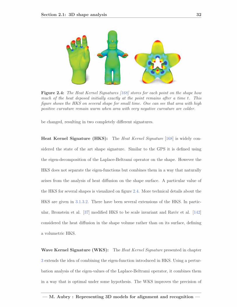
Figure 2.4: The Heat Kernel Signatures [168] stores for each point on the shape howmuch of the heat deposed initially exactly at the point remains after a time t. Thisfigure shows the HKS on several shape for small time. One can see that area with highpositive curvature remain warm when area with very negative curvature are colder.
be changed, resulting in two completely different signatures.
Heat Kernel Signature (HKS): The Heat Kernel Signature [168] is widely con-
sidered the state of the art shape signature. Similar to the GPS it is defined using
the eigen-decomposition of the Laplace-Beltrami operator on the shape. However the
HKS does not separate the eigen-functions but combines them in a way that naturally
arises from the analysis of heat diffusion on the shape surface. A particular value of
the HKS for several shapes is visualized on figure 2.4. More technical details about the
HKS are given in 3.1.3.2. There have been several extensions of the HKS. In partic-
ular, Bronstein et al. [37] modified HKS to be scale invariant and Raviv et al. [142]
considered the heat diffusion in the shape volume rather than on its surface, defining
a volumetric HKS.
Wave Kernel Signature (WKS): The Heat Kernel Signature presented in chapter
3 extends the idea of combining the eigen-function introduced in HKS. Using a pertur-
bation analysis of the eigen-values of the Laplace-Beltrami operator, it combines them
in a way that is optimal under some hypothesis. The WKS improves the precision of
— M. Aubry : Representing 3D models for alignment and recognition —

Section 2.1: 3D shape analysis 33
the HKS for matching and additionally has a natural interpretation in the framework
of Quantum Mechanics.
2.1.3 3D shape alignment methods
3D shape matching is the problem of finding a point to point correspondence between
two different shapes. There are two main approaches to tackle this problem. The
one most related to this thesis is to define for each point a descriptor that will be
discriminative but also robust to some transformations of the shape and then find a
matching that preserves L2 distance between the descriptors. Another popular strategy
is to minimize the distortion induced by the mapping. This section gives an overview
of those approaches. For a more detailed survey the reader can refer to [171] and [173].
2.1.3.1 Metric approaches
Iterative closest point methods were the first introduced to solve rigid 3D shape match-
ing [29, 41]. They were later extended to cope with some non-rigid deformations [8] by
iteratively rigidly aligning the shapes and deforming them using a non-rigid parametric
transformation. This idea however can only work with limited deformations in terms
of Euclidean distance in the 3D space.
For shape matching, the intrinsic properties of the shape, such as geodesic distances,
are more meaningful. Indeed they are mostly preserved under usual deformations. For
example, the geodesic distance between the two hands of a human body will remain
approximately the same even if their distance in the 3D space changes a lot. This leads
to the idea of viewing the shapes as metric spaces and the problem of aligning them as
finding an isometry that minimize the distance between those spaces. If the distance
— M. Aubry : Representing 3D models for alignment and recognition —

Section 2.1: 3D shape analysis 34
used is the Euclidean distance in the ambient 3D space the natural distance between
the shapes is the Hausdorff distance in the Euclidean 3D space and the standard ICP
algorithm can be used to find a locally optimal alignment. However other distances
such as the geodesic distance are more meaningful.
Using the geodesic or diffusion distance on the shapes makes the problem of finding an
optimal isometry much harder. The first challenge is to find a metric space in which
the two shapes can be meaningfully compared. Elad et al. [57] embed the shapes in
a nearly isometric way in a finite dimension Euclidean space using multidimensional
scaling (MDS) [46]. They then perform ICP in this new space and thus recover corre-
spondences between the initial shapes. However, in [57] the metric space toward which
the embedding is done and in which the Hausdorff distance is minimized is selected in
an arbitrary way. Memoli and Sapiro [125] solve this problem by applying to 3D shape
analysis the ideas of the Gromov-Hausdorff distance [78]. They compare the shapes us-
ing their isometric embedding in a metric space that minimizes the Hausdorff distance
between them. This idea was further developed for shape matching using geodesic [36]
and diffusion distances [35].
Windheuser et al. [177] use a related approach and find a deformation minimizing
the elastic energy cost of the deformation rather than the Gromov-Hausdorff distance.
Their formulation has the advantage that it leads to a binary linear program that can
be efficiently solved. Example of their results can be found in figure 2.5a
— M. Aubry : Representing 3D models for alignment and recognition —

Section 2.1: 3D shape analysis 35
(a) Shape matching minimizing theelastic energy of the deformation. Figure
from [177]
(b) Shape matching with functional mapsenforcing HKS and WKS consistency. Figure
from [136]
Figure 2.5: Shape matching by minimizing the deformation (left) and enforcing de-scriptor consistency (right)
2.1.3.2 Feature-based approaches
Inspired by the success of feature based methods in 2D alignment, many papers have
used local descriptors to match shapes. For example Gelfand et al.[72] use putative
correspondences of points with very discriminative features to propose candidate rigid
transformations and each transformation is then evaluated. The best transformation is
then used as an initialization to an ICP algorithm. Similarly Brown and Rusinkiewicz
[38] use local feature correspondences to initiate their non-rigid ICP.
An elegant way to enforce descriptor consistency in shape matching is to use the frame-
work of functional maps developed in [136]. The general idea is to formulate the prob-
lem of shape alignment as the problem of finding correspondences between the functions
on the shapes. This transforms the descriptor preservation into a linear constraint that
naturally fits into optimization. Figure 2.5b shows an example of matching with func-
tional maps. Note that functional maps used the Wave Kernel Signature introduced
in chapter 3 as point descriptor.
Other examples of feature-based 3D alignment include [88, 101, 102, 119, 137].
— M. Aubry : Representing 3D models for alignment and recognition —

Section 2.2: Instance-level 2D-3D alignment 36
All those feature-based approaches rely on the quality of the descriptor used, that must
be both robust to perturbations and discriminative between points. For this reason, a
high quality descriptor such as the Wave Kernel Signature introduced in chapter 3 is
important to all those methods.
2.2 Instance-level 2D-3D alignment
Object instance-level alignment is the problem of recovering a given object instance
in a test image together with its pose with respect to the reference representation..
The reference representation can be either a 3D model or an image. It is a difficult
problem due to the variations in the object appearance, induced by the viewpoint, the
illumination and partial occlusions (see section 1.3.2).
In this section, we present the most important methods to solve this problem. We
begin with methods based on contours, that were very popular in the early days of
computer vision. We then present local feature based methods, which are often the
most effective. Finally we present some global features that were designed to address
the sensitivity of local features to non-linear effects such as illumination effects, season
changes and depiction style.
2.2.1 Contour-based methods
2.2.1.1 Classical methods
Since its very beginning Computer Vision aligns 3D models to images. Indeed Roberts
in the abstract of his PhD in 1963 [144] explains that his ultimate goal is ”to make it
possible for a computer to reconstruct and display a three-dimensional array of solid
objects from a single photograph”. Because this objective is too complex, he restricts
— M. Aubry : Representing 3D models for alignment and recognition —

Section 2.2: Instance-level 2D-3D alignment 37
(a) Input image (b) differential image (c) reconstructed 3D solids
Figure 2.6: Object instance- level alignment by Lawrence Roberts 1963 [144]
himself to cases of objects which have a ”known three-dimensional solid”, thus being
the first to consider the 2D-3D instance alignment problem.
His work as most of the works until the nineties [129] relies on object contours. This
idea implies two main difficulties:
• to detect edges reliably.
• to aggregate the information from several edges to align the 3D model.
The problem of reliably detecting edges in cluttered scene has lead to a wide variety
of methods (eg. [40]) but is very difficult and is still open. This is one of the main
reasons why most modern alignment methods avoid explicit detection of contours by
using keypoints (see section 2.2.2) or dense representations.
To aggregate information from different edges, several methods have been developed.
In [144] Roberts uses the hypothesis of a block world to recover polygons from sets of
lines. In [89] Huttenlocher and Ullman use an hypothesis-test paradigm. They consider
the 3D model of the object known. They begin by using the edges to define keypoints
in the image based on edges corners and inflexions. They then iterate the following
procedure: (i) they use three putative correspondences between the image points and
points from the 3D model to hypothesize a pose using a weak perspective projection
— M. Aubry : Representing 3D models for alignment and recognition —

Section 2.2: Instance-level 2D-3D alignment 38
(a) Input image (b) aligned 3D instance
Figure 2.7: Instance alignment using minimal keypoint correspondence in [89]
(a) Input image (b) perceptual grouping (c) Results
Figure 2.8: Instance alignment using perceptual grouping by David Lowe [122]. Figurefrom [122].
model (i.e. a projective model with a single scale factor); (ii) they render the 3D model
from the hypothesized viewpoint and compare it to the image. They keep the proposed
detection if it is coherent with the image. The use of a set of keypoints to describe the
object makes this method invariant to some degree of occlusion, as shown in figure 2.7.
Another strategy inspired by the human ability to intuitively detect groups of edges
in an image, has been developed by David Lowe in [122]. The method uses the idea
of line grouping to hypothesize a smaller number of possible correspondences between
the image and the model. According to Lowe, the conditions that must be satisfied for
perceptual grouping are:
1. having some invariance with respect to the viewpoint
2. being unlikely in random arrangement to allow detection.
— M. Aubry : Representing 3D models for alignment and recognition —

Section 2.2: Instance-level 2D-3D alignment 39
(a) Baatz et al. [22] (b) Arandjelovic and Zisserman [11]
Figure 2.9: Recent use of contour based alignment methods for geo-localization (left)and sculpture recognition (right).
Those two points are very related to the ones we will use to define discriminative visual
elements in chapter 4. Results of this method are shown in figure 2.8.
2.2.1.2 Modern developments
While contour-based methods have been replaced for many applications and, in par-
ticular for alignment by feature-based methods, the recent literature provides a few
interesting examples where contours can be efficiently used.
First, contour-based methods perform well when the object contours can be reliably ex-
tracted both from the 2D image and the 3D model. A recent example illustrated in fig-
ure 2.9a shows that it is possible to geo-localize photographs using semi-automatically
extracted skylines matched to clean contours obtained from rendered views of digital
elevation models [22, 23].
Second, contour based alignment can produce state of the art results when the absence
of discriminative structures leads to the failure of feature based methods. This is the
case for smooth objects which is addressed in [11] and illustrated figure 2.9b. To solve
— M. Aubry : Representing 3D models for alignment and recognition —

Section 2.2: Instance-level 2D-3D alignment 40
the problem of extracting edges from real photographs, the authors present a solution
which trains a classifier that classifies super-pixels either as sculpture or not-sculpture.
Finally, contours have been successfully used to refine initial alignments provided by
features. For example Lim et al. [117] use contours to refine the pose estimation of non-
textured objects. More related to our work, Russell et al. [147] use contours to refine
the alignment between a painting and a 3D mesh reconstructed from photographs.
However, those methods require a good initialization with a close-by viewpoint.
2.2.2 Local features for alignment
Local feature descriptors summarize local image informations in regions that were
previously detected by a specific feature detector. A large variety of detectors and
descriptors exist. Selecting and describing in a robust way a set of local features in
an image has many applications. Examples include large scale 3D reconstruction and
exploration [6, 165, 166], image mosaicing [169], visual search [164], visual localiza-
tion [153], and camera tracking [26] to list but a few. Local features can also be
used for alignment as we will see in this section and for category-level recognition (see
2.3.1.1).
Local features were designed to tackle the problem of finding image to image corre-
spondences. However, their use can be extended to finding 2D-3D correspondences and
perform 2D-3D instance-level alignment [146] and retrieval [45, 140]. Large 3D scenes,
such as a portion of a city [115], can be represented as a 3D point cloud where each
3D point can be associated with local features that were used to reconstruct it [151].
2D-3D correspondences are obtained by matching the features extracted from a test
— M. Aubry : Representing 3D models for alignment and recognition —

Section 2.2: Instance-level 2D-3D alignment 41
image with the features associated to the 3D model. Standard camera resectioning can
then be used to recover the camera of the test photograph [83]. In this section, we first
introduce the main feature detectors, then feature descriptors and finally the key steps
for robust alignment.
2.2.2.1 Local region detection
The main interest for using feature detectors for alignment is to transform the problem
of finding dense correspondences between two images (or an image and a 3D model)
into the problem of finding correspondences between two sparse sets of features. The
features must be repeatable, i.e. if a region is selected in an image, the projection of
its pre-image in another image must also be detected. For this reason, those regions
are often called co-variant with respect to a family of image transformations [128].
In general, the choice of the co-variance of the detectors corresponds to a trade-off
between invariance and discriminability. Increasing the invariance of the detectors can
lead to performance losses if it is not necessary. For example, affine region detectors
work better when there is strong perspective distortion, but they are otherwise outper-
formed by circular detectors, invariant only to similarities. The region detectors that
are of most interest to us are affine-covariant detectors, because affine transformations
often approximate well the changes induced in an image by limited 3D transformations.
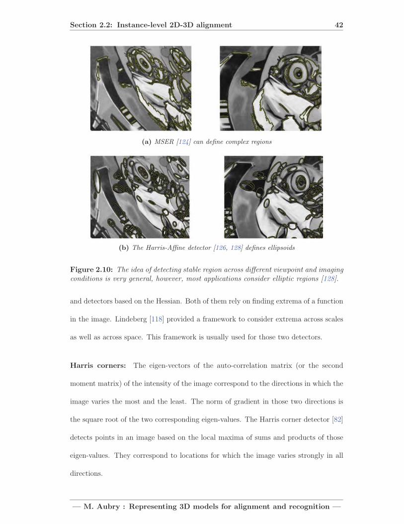
One could use any kind of regions (see figure 2.10a), but ellipsoids (see figure 2.10b) are
the most natural shapes for affine covariant regions and are used in most applications.
A good overview and evaluation of affine covariant feature detectors is available in
[128]. In this section, we discuss two of the most important detectors, Harris corners
— M. Aubry : Representing 3D models for alignment and recognition —
Section 2.2: Instance-level 2D-3D alignment 42
(a) MSER [124] can define complex regions
(b) The Harris-Affine detector [126, 128] defines ellipsoids
Figure 2.10: The idea of detecting stable region across different viewpoint and imagingconditions is very general, however, most applications consider elliptic regions [128].
and detectors based on the Hessian. Both of them rely on finding extrema of a function
in the image. Lindeberg [118] provided a framework to consider extrema across scales
as well as across space. This framework is usually used for those two detectors.
Harris corners: The eigen-vectors of the auto-correlation matrix (or the second
moment matrix) of the intensity of the image correspond to the directions in which the
image varies the most and the least. The norm of gradient in those two directions is
the square root of the two corresponding eigen-values. The Harris corner detector [82]
detects points in an image based on the local maxima of sums and products of those
eigen-values. They correspond to locations for which the image varies strongly in all
directions.
— M. Aubry : Representing 3D models for alignment and recognition —

Section 2.2: Instance-level 2D-3D alignment 43
Hessian-based detectors: Similarly, the eigen-vectors of the Hessian matrix cor-
respond to the directions with the highest and smallest curvature. The eigen-values
of the Hessian give the second derivative in both those directions. A region detector
based on those eigen-values, either by taking their sum [121], which is also the Lapla-
cian of the image, or their product [128], responds strongly to blobs and ridges. The
Laplacian can be approximated by convolving the image with a difference of Gaussians
(DoG). The DoG was the detector initially used to compute SIFT features [121]. It
can be computed efficiently using image pyramids, and approximated even faster using
integral images [174, 27].
2.2.2.2 Local region description
To be able to match the features from two images, it is necessary to describe them in a
way that is robust to perturbations induced for example by illumination changes, noise,
and small errors in the localization. Note that most of the invariance to viewpoint is
not achieved by the descriptor itself, but by the detector. As for detectors, there exists
a wide variety of descriptors. An overview and a comparison is available in [127].
Among local descriptors, some are the 2D counterpart of the descriptors presented in
2.1.2 for 3D shape matching. In particular, the idea of spin images [94] was adapted to
2D images in [109] and shape context [28] was initially developed for images, storing
the distribution of the edges given by the Canny edge detector [40].
These two descriptors belong in fact to the wide class of image descriptors using his-
tograms to describe the content of the image in the interest region. The SIFT descriptor
[121], which is arguably the most successful local descriptor, belongs to this category.
— M. Aubry : Representing 3D models for alignment and recognition —

Section 2.2: Instance-level 2D-3D alignment 44
The SIFT descriptor has been engineered to aggregate in an optimal way the gradient
orientations, using 8 orientation bins in a 4x4 grid subdivision of the region. Two of its
key ingredients are the normalization, which makes it invariant to affine illumination
changes and the limitation of the influence of strong gradients, that gives some robust-
ness to non-linear illumination effects. If the region is not a circle as in the original
paper, but an ellipsoid as in most modern algorithms, it must be normalized before the
description. Because of its success, several methods have tried to optimize further the
SIFT descriptor, for example by making its computation faster using integral images
[174, 27] or by reducing its dimension [99].
Another category of descriptors is based on computing local derivative, wavelet coeffi-
cients or in general linear filters at the interest point. It includes in particular steerable
filters [67] and complex filters [152]. These methods have had success for texture clas-
sification and similar ideas are still used in this context [161], but they proved less
robust than histogram-based methods for local region description.
Another interesting descriptor developed for texture classification called Local Binary
Pattern (LBP) [132] builds histograms of the results of binary comparisons between
pixels. Inspired by this idea, BRIEF [39] captures the local appearance in a way differ-
ent from the two previous categories of descriptors. It simply stores the binary results of
intensity comparisons between random (but fixed) pairs of points in the interest region.
One of the problems of the descriptors described above is that they remain sensitive to
appearance variations. A greater invariance can be achieved by matching the geometry
or symmetry pattern of local image features [44, 84, 158], rather than the local features
— M. Aubry : Representing 3D models for alignment and recognition —

Section 2.2: Instance-level 2D-3D alignment 45
themselves. However, such patterns are hard to detect consistently between different
views.
2.2.2.3 Robust alignment
Given two sets of image features, potential matches are given by considering for each
region in the first image the one that has the closest descriptor in the second image.
However, many of those candidate matches will be wrong. In this section, we address
the problem of recovering the good matches and the corresponding deformation be-
tween the two images from these candidate correspondences. This is typically done
[121] in two steps: first selecting the most confident matches; second computing the
most confident transformation for those matches.
Confident matches selection: The most natural way to select the most confident
matches would be to select those for which the descriptors are the closest. However,
such a method would not work because some structures are much more likely than
others and thus a descriptor can have many close descriptors which correspond to
false matches. Lowe [121] suggests to use instead the ratio between the distances of
the nearest and second nearest descriptor as an confidence score. This first-to-second
nearest neighbor distance ratio test greatly helps discarding false matches, and proves
useful in chapter 4.
Consistent transformation selection: Once the most confident matches are se-
lected, the selection can be refined further by checking the consistency between the
matches. In [121] each match defines a transformation and the Hough transform is
— M. Aubry : Representing 3D models for alignment and recognition —

Section 2.2: Instance-level 2D-3D alignment 46
used to select the most consistent one. The most popular method to check the geo-
metric consistency between matches in recent works is to perform RANSAC [64] on
the putative matches. Both methods are designed to deal efficiently with the presence
of outliers. The output of this last step is a transformation between the original 3D
model (or the original image) and the instance visible in the image.
2.2.3 Global features for alignment
The main limitation of local feature matching is its sensitivity to changes in appearance,
e.g. due to illumination, seasons, and depiction style (see figures 1.4 and 1.5). Global
descriptors of images have been developed to cope with those difficulties in the case of
scene recognition. They can also be applied to the problem of instance-level alignment
by rendering a set of views of the model and comparing them to a test image.
GIST. Those most used global feature is the GIST descriptor [133]. It divides the
image in typically 4x4 blocs and for each block stores the energy associated with
different orientations (typically 8) at different scales (typically 3). It is designed to
represent the shape of the scene and avoids looking at very local information. Thus it
is robust to important changes in the local scene appearance such as those induced by
the change of depiction style.
Exemplar-based methods. Exemplar-based methods apply to image matching the
idea developed for category-level recognition presented in section 2.3.1.2. From a single
positive example they learn a classifier [123]. If used with a descriptor of an image as
input, they have been shown to recover images of the same instance despite changes
in the depiction style [160]. This is mainly because the classifier focuses on the most
discriminative parts, which are likely to be present in all depictions of the scene. More
— M. Aubry : Representing 3D models for alignment and recognition —

Section 2.3: Category-level 2D-3D alignment 47
details on these methods are given in section 4.1.2 and 4.2.2.
2D-3D alignment with global descriptors Global descriptors are more robust to
the depiction style, but they do not handle well viewpoint changes. Thus, to align a
3D model with an image, one must compute a huge number of viewpoints of the 3D
model, and compare each rendered view with the image as was done in [147] using the
GIST descriptor.
2.2.4 Relationship to our method
The method described in chapter 4 propose an alternative approach to instance-level
2D-3D alignment. We build on the success of exemplar-based method to design a
part-based representation of the 3D model. This part based method is much more
robust to viewpoint changes than global methods. Moreover, it does not suffer from
the sensitivity of contour-based method because it is based on a soft representation of
the edges, namely HOG descriptors (see section 2.3.1.2). It also avoids the difficulty
of reliably detecting interest regions by performing dense matching instead of feature-
based matching, while keeping the robustness given by the RANSAC selection of inliers.
2.3 Category-level 2D-3D alignment
The goal of category-level 2D-3D alignment is both to recognize an object from a given
category in a test image and to output a 3D model aligned with the image. Until
recently this problem has received little attention. Category recognition was rather
performed using purely 2D methods. However these 2D methods implicitly handle
the fact that the object appearance varies with the viewpoint and they can be used
— M. Aubry : Representing 3D models for alignment and recognition —

Section 2.3: Category-level 2D-3D alignment 48
to recover the viewpoint if enough training data is available. For this reason, we will
begin by reviewing 2D category-level recognition methods and then present the more
recent work on 2D-3D category-level alignment.
2.3.1 2D methods
2.3.1.1 Bag of features
It is possible to describe the content of an image using the local features present in
this image (introduced in section 2.2.2). This approach was introduced by Csurka et
al. [48] and Opelt et al. [134]. A detailed evaluation of ”Bag of features” methods is
presented in [184] and shows that they are surprisingly robust to intra-class variation,
which is one of the main difficulty of category-level recognition compared to instance-
level recognition. The typical pipeline for a ”Bag of features” recognition pipeline is
as followed. First, local features such as affine SIFTs are extracted from all training
images. They are then aggregated in an histogram defined using a codebook called
visual vocabulary learned from all images. Finally a classifier, typically a linear SVM,
is learned to differentiate between the histograms of the different classes. This approach
has been extended to encode spatial information using a spatial pyramid in [110] and
can be used a global descriptor (see section 2.2.3).
2.3.1.2 Single template method
Bag of features methods are based on the aggregation of local features. On the con-
trary one can represent an object by a single template or a small set of templates
corresponding to the different possible viewpoints of the object. This idea was applied
successfully in [49] to pedestrian detection, using histograms of oriented gradients or
HOGs and a linear SVM classifier. The HOG descriptor is very similar to the SIFT
— M. Aubry : Representing 3D models for alignment and recognition —

Section 2.3: Category-level 2D-3D alignment 49
Figure 2.11: The HOG descriptor [49] summarizes the local gradient orientations.
Figure 2.12: The SVM in the HOG-SVM pipeline [49] emphasizes the importantgradient orientations. (a) Average gradient for the pedestrian category. (b) and (c)Positive and negative SVM weights for each HOG cell. (d) Test image. (e) HOGdescriptor of the test image. (f) and (g) HOG descriptor of the image weighted by thepositive and negative SVM weights. Figure from [49].
descriptor [121] but is designed to be computed densely over an image. Each HOG cell
essentially represents in a robust way the dominant gradient orientations as visualized
in figure 2.11. The SVM weights the contribution of the different cells and orientations,
emphasizing the important gradients for the category as shown in figure 2.12.
2.3.1.3 Deformable parts model (DPM)
Fischler and Elschlager [65] introduced the idea of defining a pictorial structure to
describe the arrangements of parts of an object, as shown for example on figure 2.13.
This idea was revisited in [62] and made popular by Felzenszwalb et al. [61]. They train
a latent-SVM model using HOG features to create a state-of-the-art method for object
category detection. Deformable part models represent an object by a root HOG and
parts represented by HOGs at twice the resolution of the root HOG. The detectors for
the root and parts as well as their locations and weights in the final score are learned
— M. Aubry : Representing 3D models for alignment and recognition —

Section 2.3: Category-level 2D-3D alignment 50
Figure 2.13: The idea of pictorial structures [65] is to represent an object categoryby a set of parts with constraint relative locations. Figure from [65]
Figure 2.14: Deformable part models capture jointly the appearance of object partsfor several viewpoints. Figure from [61].
jointly.
The 3D variations of the object appearance is handled by DPM by considering several
models corresponding to different aspect ratios for each object category and by allowing
the parts to move with respect to the root with a Gaussian deformation cost.
— M. Aubry : Representing 3D models for alignment and recognition —

Section 2.3: Category-level 2D-3D alignment 51
Figure 2.15: Architecture of the convolutional neural network used by Krizhevsky etal. [107] for object classification. Figure from [107]
Figure 2.16: Detection pipeline proposed by Girshick et al. [75]. Figure from [75].
2.3.1.4 Convolutional neural networks
Recently, DPMs have been outperformed by deep learning methods. Convolutional
neural networks [111] are formed by a succession of convolutions, rectifying non-linear
units (ReLU), max poolings and local normalizations (see figure 2.15). They had al-
ready shown impressive and practical results on optical character recognition [112, 162],
but until recently their performance for other vision task was limited by the available
training data and computational power. The developpement of GPU computing and
the appearance of the large scale ImageNet dataset [54] allowed Krizhevsky et al. [107]
to develop a network architecture, shown in figure 2.15, that outperforms by a signif-
icant margin other methods for image classification. This method was extended into
a state of the art method for object detection in [75] using a fine-tuned version of the
initial network to classify warped candidate regions as shown figure 2.16. Interestingly,
and related to the work on non-realistic depictions presented in chapter 4, CNNs have
also been shown to perform well for object-category classification in paintings [47].
— M. Aubry : Representing 3D models for alignment and recognition —

Section 2.3: Category-level 2D-3D alignment 52
Figure 2.17: Detection of block-like objects by Xiao et al. [180]. Figure from [180].
Figure 2.18: Xiang et al. [179] approximate objects by set of planes. Figure from[179].
2.3.2 3D methods
Recently several papers aimed at using 3D information to perform category level recog-
nition and alignment. Two main research directions have been explored
The first way to tackle the problem is to make simplifying and non-realistic hypothesis
about the 3D content of the world, revisiting the ”block world” methods of the early
days of computer vision. This has been explored for buildings in outdoor scenes in
[79] and for box-like objects in indoor scenes in [63, 180]. An example of the results
of those methods is shown figure 2.17. This approach was extended to more complex
shapes than blocks either by designing manually object models using a combination
of blocks [42, 53] or by learning an approximation of the layout of an object category
using a set of planes [179] as shown figure 2.18. Using a non-parametric approach [150]
showed promising results, but is designed to work in highly structured scenes.
Another way to approach the problem is to extend to 3D the ideas of the DPM [62],
— M. Aubry : Representing 3D models for alignment and recognition —

Section 2.3: Category-level 2D-3D alignment 53
Figure 2.19: The idea of extending DPMs to 3D, here in the framework of Hejratiand Ramanan [85]. Figure from [85].
which have been very successful for 2D object recognition. This idea is visualized
figure 2.19. For example [185] uses manually labelled points on 36 car models to learn
a deformation model of the shape and the local appearance. Glasner et al. [76] have
a slightly different approach and used patches from images of 22 registered models of
cars to vote for the location and orientation. Other examples include [85, 138, 185].
More recently Yang et al. [182] attempted to extend CNN for viewpoint estimation.
Those methods use a relatively small number of models and typically focus on objects
with a simple geometry or a limited intra-class variation such as cars. They also often
require manual annotation of 3D key-points that are used to represent the shape of the
objects and train detectors.
2.3.3 Relationship to our method
In chapter 5 we present a data-driven part-based method to tackle the problem of 3D
category-level recognition. Opposite to previous methods which typically use simple
3D models, we use the complex “chair” category that we represent using more than
thousand 3D models collected from the Internet and more than 80 000 rendered views.
While we use a star star-model similar to the DPM approach, we also use an exemplar-
based method to avoid the need of large collections of annotated images to learn our
model. Finally, our approach has the new advantage that given an input image it
— M. Aubry : Representing 3D models for alignment and recognition —

Section 2.3: Category-level 2D-3D alignment 54
returns a 3D model from our shape collection similar to the depicted object and aligned
with the image.
— M. Aubry : Representing 3D models for alignment and recognition —

55
Chapter 3
Wave Kernel Signature
3.1 Introduction
In this chapter, we are interested in developing a local descriptor that enables robust
and accurate matching between two meshes representing the same 3D object. This
local descriptor is illustrated figure 3.1. We place ourself in the context of the har-
monic analysis of shapes introduced in 2.1.2.2 and design the Wave Kernel Signature
(WKS). It aims at achieving an optimal trade-off between robustness and accuracy
by studying the influence of perturbations in the metric on the eigen-values of the
Laplace-Beltrami operator. The WKS has a natural interpretation in the framework of
Quantum Mechanics. It represents the time-averaged probability of measuring a quan-
tum mechanical particle at a specific location on the shape. By considering particles
of varying energy distribution, the WKS encodes and separates information from the
different Laplace eigenfrequencies. Both theoretically and in quantitative experiments
we demonstrate that the WKS is substantially more discriminative and therefore leads
to better feature matching than the commonly used Heat Kernel Signature (HKS). We
also show that the WKS can be used for other applications such as shape segmentation
— M. Aubry : Representing 3D models for alignment and recognition —

Section 3.1: Introduction 56
Figure 3.1: Schrodinger’s cat [154] and its Wave Kernel Signatures. Based on theSchrodinger equation each point on an object’s surface is associated with a Wave KernelSignature. Note that the signature captures shape variations in the environment of theconsidered point at various spatial scales: While the two points of the bottom are quitesimilar for large scales (small values of the energy), the two others are quite different.
and recognition.
3.1.1 Motivation
The analysis of shape plays a central role in computer vision and beyond. To analyze
and compare 3D shapes is by no means straight-forward. Even the computation of
a distance between two given 3D shapes leads to NP-hard combinatorial problems
[36, 125, 177] (see section 2.1.3.1).
As mentioned in section 2.2.2 local descriptors have drastically improved and simplified
many computational challenges for images, in particular alignment problems. Algo-
rithms for image matching, correspondence finding, camera pose estimation, tracking
and recognition have substantially gained in speed and real-world performance by rely-
ing on local invariant descriptors such as SIFT [121] (see section 2.2.2). The enormous
number of citations to these works indicates the practical relevance of such feature
descriptors. In analogy, appropriate feature descriptors for 3D shapes will facilitate
their analysis, improving and accelerating shape matching, shape recognition, shape
— M. Aubry : Representing 3D models for alignment and recognition —

Section 3.1: Introduction 57
retrieval and shape decomposition.
As explained in 2.1.2 a shape descriptor assigns a signature to each point of a 3D
shape characterizing this point with respect to the full shape. This signature should
be invariant or robust to certain transformations and perturbations, yet it should be
discriminative in the sense that corresponding points on the two shapes should be
assigned similar signatures and points not in correspondence should have different
signatures. As discussed in section 2.1.3.2, having a good feature descriptor for 3D
shapes would simplify many challenges and in particular alignment.
In this chapter, we introduce a novel highly discriminant feature descriptor for 3D
shape analysis which is based on a quantum mechanical treatment of shape.
3.1.2 From Quantum Mechanics to shape analysis
The mathematical models employed for the analysis of images and shapes are frequently
inspired from physics. The curve evolutions employed for segmentation and tracking
in [31], for example, were inspired by Newtonian equations of motion. The theory
of Fourier analysis and frequency decompositions originated with Fourier’s studies of
heat propagation. The heat equation itself stands at the origin of nonlinear diffusion
filtering [139, 176]. The process of heat diffusion also inspired the derivation of the
Heat Kernel Signature (HKS) as a feature descriptor for 3D shapes [168]. The central
physical analogy underlying this signature is to place a source of heat at a given point
of the 3D shape and to study how the heat diffuses over time.
A mathematical framework which has attracted fairly little attention in the analysis
of images or shapes is that of Quantum Mechanics. Although Quantum Mechanics
revolutionized the mathematical modeling of microscopic physical phenomena at the
beginning of the 20th century, the respective mathematical models have not been ap-
— M. Aubry : Representing 3D models for alignment and recognition —

Section 3.1: Introduction 58
plied much in image or shape analysis. A notable exception is the use of Schrodinger’s
equation and complex diffusion for image denoising and image enhancement [74].
The theory of Quantum Mechanics has many facets and a complete review is beyond
the scope of this thesis. For an excellent introduction the reader is referred to [149].
In this paper, we will show how a family of shape descriptors can be interpreted in the
framework of Quantum Mechanics and introduce a new feature descriptor called the
Wave Kernel Signature which exhibits several advantages over the frequently used Heat
Kernel Signature. The central physical analogy we propose is that we place a quantum
mechanical particle on a 3D shape and determine the time-averaged probability of
observing this particle in a given location. The Wave Kernel Signature assigns to each
point on the surface a vector containing the time-averaged probability for locating
particles of different energy. While the process of heat diffusion underlying the HKS
converges over time to a steady state, the evolution of quantum mechanical particles
underlying the WKS is governed by Schrodinger’s equation and does not converge to
a steady state. Therefore time averaging provides a meaningful quantity. In fact,
through the time-averaging the notion of time actually disappears such that the WKS
is a signature associated with a stationary analysis of shape.
As we will show in section 3.1.3.3 and 3.3.2, the HKS and the underlying heat diffusion
process tend to merge shape information on different spatial scales (or frequencies). In
contrast, the WKS nicely separates shape information on different scales. Moreover, we
demonstrate that the Wave Kernel Signature is superior to the Heat Kernel Signature
and its variants as it allows a better discrimination of points on the shape and a more
accurate localization of correspondences.
In the following we well give a review of the mathematical framework of spectral meth-
— M. Aubry : Representing 3D models for alignment and recognition —
Section 3.1: Introduction 59
ods in the context of 3D shape analysis. We will then introduce a family of shape
descriptors, the Wave Kernel Signature which generalizes the Heat Kernel Signature.
Next, we derive a particularly well-suited choice of the WKS and we derive some of
its mathematical properties. Finally we will show in an extensive experimental evalua-
tion that the Wave Kernel Signature has a favorable performance compared to existing
feature descriptions such as the Heat Kernel Signature and its derivatives.
3.1.3 Spectral Methods for shape analysis
Because of its interesting properties mentioned in 2.1.2.2, techniques relying on the
spectral decomposition of the Laplace–Beltrami operator have become in recent years
fundamental in data analysis [108] and more specifically in shape analysis [114]. In this
section we will briefly review the mathematical background of the Laplace–Beltrami
operator on surfaces and the relation of its spectral decomposition to classical Fourier
analysis. Next, we will recall the definition and the main properties of the Heat Kernel
Signature (HKS) [168]. Finally, we will perform a spectral analysis of HKS which
indicates that despite its theoretical elegance, HKS does not organize the information
on points in an optimal way.
3.1.3.1 The Laplace–Beltrami operator and PDEs on surfaces
Let X ⊂ R3 be a closed differentiable surface, and let g denote the Riemannian metric
on X which is induced by the embedding in the Euclidean R3. The Laplace–Beltrami
operator is a linear second-order differential operator
Δ : L2(X) → L2(X). (3.1)
— M. Aubry : Representing 3D models for alignment and recognition —

Section 3.1: Introduction 60
For a function f ∈ C2(X;R), it is defined as
Δf = div(grad f). (3.2)
In local coordinates x1, x2 with metric tensor g = gij, inverse metric tensor gij, and
metric determinant det(g) = |g|, the Laplace–Beltrami operator is given by
Δf =1√|g|
∂
∂xi
(√|g|gij ∂
∂xjf
). (3.3)
The Laplacian is a negative, self-adjoint operator on L2(X). If X is compact, Δ admits
a discrete spectral decomposition. Let 0 = −E0 > −E1 ≥ . . . be the eigenvalues of Δ,
denote by φ0, φ1, . . . the corresponding L2-normalized eigenfunctions. In other words,
the φk satisfy Helmholtz’ equation
Δφk = −Ekφk. (3.4)
Note that E0 = 0 because the constant functions are solutions of the equation with
eigenvalue 0 and that the φk are defined only up to an orthogonal transformation of
the eigenspaces.
The functions φk are the natural generalization to surfaces of the classical Fourier ba-
sis√2 sin(nπx),
√2 cos(nπx) which solve Helmholtz’ equation on the unit circle S1. In
paricular, they can be thought of as vibration modes: The value of an eigenfunction φk
in a point represents how much it moves in the vibration mode, and the correspond-
ing eigenvalue is minus the square frequency of vibration. This (classical) mechanical
interpretation of the eigenvectors gives a first intuition about them, in particular eigen-
vectors that vary fast spatially are also the ones with high frequency, as can be seen in
— M. Aubry : Representing 3D models for alignment and recognition —

Section 3.1: Introduction 61
Figure 3.2: First and 300th eigenfunction of the Laplace-Beltrami operator. Thecolors represent the values of the eigenfunctions, blue being the most negative and redthe most positive value. The eigenfunctions can be thought of as vibration modes, withlow frequencies having slow spatial variation, and high frequencies having fast spatialvariation.
Fig. 3.2. This connection between frequencies of the Laplace-Beltrami operator and
spatial scales will be important for understanding the scale separation properties of
respective 3D shape signatures.
The classical Fourier decomposition allows to develop any periodic signal f , that is any
signal defined on S1 in its frequency components
f(x) =∑k
ak√2 cos(πkx) + bk
√2 sin(πkx), (3.5)
where
ak =
∫S1
f(x)√2 cos(πkx)dx,
bk =
∫S1
f(x)√2 sin(πkx).
(3.6)
Similarly, given a signal f : X → R defined on X, we can decompose f into its
frequency components
f =∑k≥0
ckφk, (3.7)
where ck =∫Xf · φk.
— M. Aubry : Representing 3D models for alignment and recognition —

Section 3.1: Introduction 62
Given a point x ∈ X, the Dirac delta function corresponding to x is the distribution
defined by
δx : C∞(X) → R, f �→ f(x). (3.8)
The point x is uniquely determined by its delta function. As a generalized signal on
X, δx can be decomposed into its frequency components. The Fourier coefficients of
δx are given by
ck =
∫X
δx(y)φk(y)dy = φk(x). (3.9)
With this in mind, it is tempting to define a feature descriptor for points on surfaces
simply by concatenating the Fourier coefficients ck into a vector indexed over k. Up to a
multiplicative factor in each component, this is exactly the idea underlying the Global
Point Signature (GPS) defined by Rustamov [148]. Indeed, this signature characterizes
points uniquely up to isometry. Unfortunately, the coefficients ck depend on the choice
of the sign of the Laplace eigenfunctions φk. In the case of repeated eigenvalues, the
situation becomes even worse because the coefficients are only determined up to an
orthogonal transformation of the eigenspace. As a consequence, a different choice of
basis functions may lead to an entirely different signature.
3.1.3.2 The Heat Kernel Signature
The HKS overcomes these difficulties in a very elegant way. As indicated by the name,
it relies on the diffusion of heat on the surface. Given an initial heat distribution
u0 : X → R, the heat distribution u(·, t) : X → R for times t > 0 solves the heat
equation ⎧⎪⎪⎪⎨⎪⎪⎪⎩∂u(x, t)
∂t= Δu(x, t),
u(x, 0) = u0(x).
(3.10)
— M. Aubry : Representing 3D models for alignment and recognition —

Section 3.1: Introduction 63
HKS scaled-HKS WKS
Figure 3.3: Comparison of the Heat Kernel Signature (first column), the scaled HeatKernel Signature (second column) and the Wave Kernel Signature (third column) fortwo different points (first and second line) and two different shapes (red and blue).Note that while remaining robust to deformations the WKS captures more informationincluding shape differences at finer scales.
The fundamental solution to the heat equation is given by the heat kernel K : X ×
X × R>0 → R defined by
K(x, y, t) =∑k≥0
e−Ektφk(x)φk(y). (3.11)
Thus, equation (3.10) is solved by
u(x, t) =
∫X
K(x, y, t)u0(y)dy. (3.12)
The Heat Kernel Signature at a point x ∈ X is based on the following physical ex-
periment: Assume that initially at time t0 = 0 an infinite amount of heat is placed
at x and that there is no heat on X \ {x}, corresponding to a Dirac delta function δx
as initial heat distribution. Let this initial distribution diffuse and define the HKS at
x and time t > 0 as the amount of heat remaining in x at time t. According to the
— M. Aubry : Representing 3D models for alignment and recognition —

Section 3.1: Introduction 64
above, the HKS can be computed as
HKS(x, t) =
∫X
(∑k≥0
e−Ektφk(x)φk(y)δx(y)
)dy
=∑k≥0
e−Ektφk(x)2. (3.13)
Sun et al. [168] introduced this signature as a point descriptor and showed that points
on a 3D shape are almost completely characterized by their HKS (see Section 3.3.3
for the precise statement in the analogous case of WKS). Moreover, being the result
of a physical experiment, HKS does not depend on the signs or on the ordering of the
Laplace eigenfunctions. This can also be read off directly from formula (3.13).
Sun et al. [168] noticed that the HKS tends to decrease exponentially, as can be seen
in figure 3.3. Thus, they introduced a heuristic modification of the HKS to avoid this
effect, that we will refer as sHKS:
sHKS(x, t) =HKS(x, t)∫
XHKS(y, t)dy
(3.14)
One of the main drawbacks of this descriptor is that it is not invariant to scale. For this
reason Bronstein and Kokkinos [37] introduced the scale-invariant heat kernel signature
(SI-HKS) which makes the HKS invariant to scale using logarithmic sampling and
Fourier transform.
3.1.3.3 Limitations of the HKS
Despite its elegant physical derivation and its appealing theoretical properties, the
HKS has a number of practical drawbacks. In order to discuss these, we come back to
the signal-theoretic interpretation of φk(x) as the k-th Fourier coefficient of the delta
function δx. From this point of view, HKS(x, t) is an expression in the squared Fourier
— M. Aubry : Representing 3D models for alignment and recognition —

Section 3.2: The Wave Kernel Signature 65
(a) HKS (b) WKS
Figure 3.4: This figure shows the weight given by the HKS and WKS (blue andred lines) to the coefficients (black spikes) corresponding to the different energies (xaxis). The weighting of WKS is more intuitive and discriminative since it aggregatesinformation only from similar eigenvalues.
coefficients of δx. More precisely, (HKS(x, t))t>0 can be seen as a collection of low-pass
filters applied to δx: for large t, the high frequencies are suppressed – see Figure 3.4.
This brings about the following disadvantages of the HKS:
• With increasing time t, the HKS mixes information from all scales. Separating
shape differences on different spatial scales is not possible.
• Regardless of the choice of t > 0, HKS(x, t) is dominated by low frequency
information, which corresponds to global properties of the shape.
3.2 The Wave Kernel Signature
3.2.1 From heat diffusion to Quantum Mechanics
The above limitation of the HKS is inherently tied to the process of heat diffusion,
where for larger values of time t, the heat distribution invariably converges to an
entirely uninformative constant temperature. Can we overcome this limitation of the
— M. Aubry : Representing 3D models for alignment and recognition —

Section 3.2: The Wave Kernel Signature 66
HKS by reverting to a different physical process? Can we rely on another mathematical
equation whose solution would not be dominated by the global properties of the shape
which are embedded in the eigenfunctions associated with the large frequencies?
We would like to adhere to the Laplace-Beltrami operator because of its favorable
properties, its eigenfunctions being associated with frequencies of vibration [97] as
visualized in figure 3.2. Yet, we would like a physical process which does not attenuate
the high frequencies as the heat diffusion does.
A mathematical solution is to multiply the Laplace-Beltrami operator by the imaginary
number ’i’. That way the eigenvalues of the operator are complex and the contribution
of the different frequencies will not be attenuated over time. The resulting equation is
a specific case of the Schrodinger equation, which describes the behavior of a quantum
particle. The state of the quantum particle at time t is fully described by the complex
function ψ(·, t), often referred to as the wave function. In particular, the squared norm
|ψ(x, t)|2 of the wave function corresponds to the probability density for detecting the
particle at a location x at time t. The evolution of a particle described at t = 0 by the
function ψ0 is governed by the equation:
⎧⎪⎪⎪⎨⎪⎪⎪⎩i∂
∂tψ(x, t) = Hψ(x, t) = (−Δx + V (x)) ψ(x, t),
ψ(x, 0) = ψ0(x).
(3.15)
Here H = −Δ + V is called the Hamiltonian operator, and V (x) is a real potential
representing an external field – for example an electric field – acting on the particle.
For simplicity, we assume this external field to be constant in time. In Section 3.2.4,
we will discuss how to exploit such an external field in order to constrain particles to a
certain spatial vicinity, thereby localizing the shape analysis and allowing a multiscale
— M. Aubry : Representing 3D models for alignment and recognition —

Section 3.2: The Wave Kernel Signature 67
analysis of shapes.
3.2.2 Schrodinger equation on a surface
To solve the Schrodinger equation we can exploit the fact that the Hamiltonian op-
erator H = −Δ + V is compact and self-adjoint on the Hilbert space of complex L2
functions on X. According to the spectral theorem we can therefore diagonalize it in
an orthonormal basis. Let (φ0, φ1, ...) denote a basis of eigenfunctions of the operator
H, and let (E0, E1, ...) denote the corresponding eigenvalues. We can further assume
that E0 ≤ E1 ≤ .... For simplicity we assume that there are no degeneracies, i.e. that
the eigenvalues are distinct, which is the general case.
To solve the Schrodinger equation (3.15), we simply expand the solution ψ(x, t) in the
basis (φ0, φ1, ...):
ψ(x, t) =∞∑k=0
fk(t)φk(x), (3.16)
where
fk(t) =
∫X
φk(x)ψ(x, t) dx
denotes the k-th frequency component at time t. Inserting this basis expansion in
(3.15), we get:∞∑k=0
d
dtfk(t)φk(x) =
∞∑k=0
iEk fk(t)φk(x) (3.17)
Since (φ0, φ1, ...) is an orthogonal basis, we can solve in each coordinate separately,
and thus the solution is given by
ψ(x, t) =∞∑k=0
fk(0) eiEktφk(x) (3.18)
The expected value of the Hamiltonian H provides the energy of a particle in a state
— M. Aubry : Representing 3D models for alignment and recognition —

Section 3.2: The Wave Kernel Signature 68
ψ(x) by∫SψHψ. The only possible output in the measurement of the energy are the
eigen-states of H, and the probability to find an energy Ek (assuming that all the
eigen-energies are distinct) is given by∫SφkHψ. Thus the φk are also known as energy
eigen-states, since a particle in the state φk will always be measured to have an energy
Ek.
3.2.3 A spectral signature for shapes
The remaining task is to derive a signature which characterizes points on the 3D shape
based on the physical process of quantum particle evolution described by equation
(3.15). This task can be decomposed into two aspects:
• Choose an initial distribution of energy.
• Choose a quantity to consider/measure.
For the HKS, the signature of a point was determined by using the evolution of the
temperature on a point with a Dirac distribution in this point at t = 0. The intuition
was that for small time, the solution was influenced mainly by the local shape, and
that the signature grew more global with time. Nevertheless, the study of the equation
showed that a transparent interpretation in terms of scale is not obvious given that
different frequencies are increasingly mixed and the small eigenvalues dominate. In
practice researchers compensated this dominance of small eigen-values at larger times
by introducing a logarithmic sampling of time.
In the following, we therefore suggest to parameterize the shape descriptor not as a
function of time, as done in the HKS, but as a function of the energy of the particle.
This will give rise to a new feature descriptor which we call the Wave Kernel Signature
(WKS). While it is also derived from a physical process, the WKS is a time-independent
— M. Aubry : Representing 3D models for alignment and recognition —

Section 3.2: The Wave Kernel Signature 69
signature. More specifically denote the energy distribution of the quantum mechanical
particle by fk(0) = fE(Ek) (E will be the parameter of the distribution, see Section
3.3.1 for the exact choice of this distribution).
Definition 1. The Wave Kernel Signature (WKS) associated with a given point x ∈ X
is the time-averaged probability of detecting a particle of a certain energy distribution
fE at that point. Mathematically, it can be computed as:
WKS(x,E) = limT→∞
1
T
∫ T
0
|ψ(x, t)|2dt
= limT→∞
1
T
∫ T
0
∣∣∣∣∣∞∑k=0
fE(Ek)φk(x)eiEkt
∣∣∣∣∣2
dt
= limT→∞
1
T
∫ T
0
∞∑k,l=0
fE(Ek)φk(x)fE(El)φl(x)eiEkte−iEltdt
=∞∑
k,l=0
fE(Ek)φk(x)fE(El)φl(x) limT→∞
1
T
∫ T
0
eiEkte−iEltdt
(3.19)
As a result, we obtain:
WKS(x,E) =∞∑k=0
|fE(Ek)|2|φk(x)|2. (3.20)
The last equality holds because limits can be exchanged. While respective limits do
not generally commute, they do in our case for a large range of functions fE (including
Gaussians and exponentials) since as shown in [86]:
||φk||∞ ≤ CE14k (3.21)
The above definition of the Wave Kernel Signature is very general: the function fE can
be chosen in many ways leading to different kinds of signatures. In this chapter we use
a general stability analysis of the shape as detailed in section 3.3 to derive a particular
— M. Aubry : Representing 3D models for alignment and recognition —

Section 3.2: The Wave Kernel Signature 70
fE. Our result is also physically meaningful since it corresponds to a particle which
energy has been measures with a log-normal error. Bronstein [120] later suggested this
function could be learned to optimize some task on a specific dataset. 3.3.1.
Proposition 1. The family of descriptors introduced in Definition 1 is a generalization
of the Heat Kernel Signature.
Proof. For the choice of an exponential energy distribution
fE(Ek) = e−√Ekt,
the WKS in (3.20) is equivalent to the HKS in (3.13).
3.2.4 Global vs. local WKS
In our original article [21], the Schrodinger equation was used without potential, and
thus the signature of each point depended on the entire shape. Adding a spatial po-
tential V forces particles with low energy to stay in some part of the shape. As a
consequence, one can design a shape signature which will only be affected by a prede-
fined local neighborhood. For example, to describe a point x the following potential
can be used:
Vx(y) =
⎧⎪⎪⎨⎪⎪⎩
0 if d(x, y) ≤ d0
∞ if d(x, y) > d0
(3.22)
where d is the geodesic distance between two points of the shape and d0 is a reference
distance. The corresponding local descriptor will no longer be scale invariant (since a
reference distance will be introduced in the potential), but it will be more suitable for
partial shape matching where local parts should be identified as similar even if their
relation to the remainder of the shape is very different. The appropriate scale can
— M. Aubry : Representing 3D models for alignment and recognition —
Section 3.3: Mathematical Analysis of the WKS 71
be chosen using some property of the shape. Alternatively one can sample numerous
scales in a logarithmic manner leading to a full multi-scale description of the shape.
An example of such a local descriptor is given in 3.4.1.2. In the rest of this chapter,
we focus on the case of a constant potential.
3.3 Mathematical Analysis of the WKS
In this section we will present a mathematical analysis of the Wave Kernel Signature
introduced above. In particular, we will perform a theoretical stability analysis which
justifies the choice of the log-normal distribution for the energy levels in the definition
of WKS. Next, we will argue that in contrast to the HKS, the WKS ensures a clear
separation of scales. Finally, we will summarize the favorable properties of WKS
concerning its invariance to non-rigid deformations as well as its discriminative power.
3.3.1 Stability analysis
In this subsection, we derive an adapted energy distribution fE for a particle on the
surface with expected energy level E. By better understanding how the spectral de-
composition of the shape varies with small deformations, we will be able to design a
descriptor that will be both informative and robust to small non-isometric perturba-
tions of the considered surface.
Assume that a surface X is slightly deformed in a non-isometric way. Mathematically
we can interpret such a deformation as a perturbation g(ε) of the metric g = g(0) on X
for a real parameter ε with |ε| small. Assume that the deformation is regular in the sense
that g(ε) = g(0) + εg1 + ε2g2 + . . . and the corresponding Laplace–Beltrami operators
Δ(ε) = Δ(0) + εΔ1 + ε2Δ2 + . . . depend analytically on ε (compare also [143, Def. 3]).
— M. Aubry : Representing 3D models for alignment and recognition —

Section 3.3: Mathematical Analysis of the WKS 72
For simplicity, we assume that the Laplace–Beltrami operator Δ(0) corresponding to
g(0) has no repeated eigenvalues. By [143, prop. 2], for each eigenvalue −Ek of Δ(0),
there exists an analytic family Ek(ε) with Ek(0) = Ek and −Ek(ε) in the spectrum of
Δ(ε).
Theorem 1. Denote by C = ||g1||g(0) the first order norm of the metric deformation,
where the space of symmetric tensors TX∗ ⊗ TX∗ is endowed with the norm induced
by g(0). Then for |ε| > 0 sufficiently small we have
|Ek(ε)− Ek| ≤ CEk · |ε|+O(ε2).
Proof. Denote by φk(ε) the normalized eigenfunctions to the eigenvalue Ek(ε). By
[143], we have
φk(ε) = φk(0) +O(ε). (3.23)
Let ak,i(ε) = 〈φk(ε), φi(0)〉L2(X). Then
φk(ε) =∑i
ak,i(ε)φi(0) (3.24)
and by (3.23) we can infer that
ak,k = O(1), ak,i = O(ε) for i = k. (3.25)
Now, we plug this into the eigenvalue equation
Δ(ε)φk(ε) = Ek(ε)φk(ε). (3.26)
— M. Aubry : Representing 3D models for alignment and recognition —

Section 3.3: Mathematical Analysis of the WKS 73
On the left hand side of (3.26) we get
(Δ(0) + εΔ1 +O(ε2)
)(∑i
ak,i(ε)φi(0))
= Ek(0) · ak,k(ε)φk(0)
+ εak,k(ε)Δ1 (φk(0)) +
∑i �=k
ak,i(ε)Ei(0)φi(0)
+O(ε2).
(3.27)
The right hand side of (3.26) is equal to
Ek(ε) ·(ak,k(ε)φk(0) +
∑i �=k
ak,i(ε)φi(0)). (3.28)
Now we take on both sides the L2(X)-scalar product with φk(0) to obtain
ak,k(ε)Ek(0) + εak,k(ε)
∫X
φk(0)Δ1 (φk(0)) +O(ε2)
= Ek(ε)ak,k(ε).
(3.29)
Since ak,k(ε) = 0 for |ε| sufficiently small, we get
Ek(ε) = Ek(0) + ε
∫X
φk(0)Δ1 (φk(0)) +O(ε2). (3.30)
Thus, we have to show that
∣∣∣∣ε∫X
φk(0)Δ1(φk(0))
∣∣∣∣ ≤ CEkε+O(ε2). (3.31)
— M. Aubry : Representing 3D models for alignment and recognition —

Section 3.3: Mathematical Analysis of the WKS 74
Since εΔ1 = Δ(0)−Δ(ε) +O(ε2), we get
∣∣∣∣ε∫X
φk(0)Δ1(φk(0)
)∣∣∣∣=
∣∣∣∣∫X
φk(0)(Δ(0)−Δ(ε)
)(φk(0)
)∣∣∣∣+O(ε2)
≤∫X
∣∣∣g(0)(dφk(0), dφk(0))− g(ε)
(dφk(0), dφk(0)
)∣∣∣+O(ε2)
(3.32)
where we used Gauss’ theorem on surfaces. Now, g(0) − g(ε) = εg1 + O(ε2). On
the other hand, for all v ∈ Rn, A ∈ R
n,n we have∣∣〈v, Av〉∣∣ ≤ ‖A‖F · 〈v, v〉, where
‖ · ‖F denotes the Frobenius norm. This implies that∣∣g1(α, α)∣∣ ≤ C · g(0)(α, α) for all
1-forms α on X. Thus,
∣∣∣∣ε∫X
φk(0)Δ1(φk(0)
)∣∣∣∣≤
∫X
∣∣εg1(dφk(0), dφk(0))∣∣+O(ε2)
≤ |ε| · C ·∫X
g(dφk(0), dφk(0)
)+O(ε2)
= |ε| · CEk +O(ε2).
(3.33)
This concludes the proof.
The theorem implies that there exist ck with |ck| ≤ C such that
Ek(ε) = (1 + εck)Ek +O(ε2).
— M. Aubry : Representing 3D models for alignment and recognition —

Section 3.3: Mathematical Analysis of the WKS 75
This can be reformulated as
log
(Ek(ε)
Ek
)= log(1 + εck +O(ε2)) = εck +O(ε2). (3.34)
For convenience, we model the ck coefficients by independent normally distributed
random variables:
log(Ek(ε)) ∼ N (log(Ek), σ). (3.35)
Thus, in our model, the eigen-energies of an articulated shape X are log-normally
distributed random variables. We design our descriptor to take into account this infor-
mation without any assumption about the variations of the eigenfunctions.To achieve
this, we choose f 2E as a log-normal distribution.
WKS(x, e) =∞∑k=0
e−(e−log(Ek))2
2σ2 |φk(x)|2 (3.36)
In this equation the parameter σ allows an intuitive trade-off between discrimination
(σ → 0) and robustness to deformations (σ → ∞).
Note that this formulation also provides a very meaningful interpretation in the Quan-
tum Mechanics framework: suppose that the log-energy e of a particle is measured with
a Gaussian error of variance σ, the average probability to measure it in x is WKS(x, e).
3.3.2 Spectral analysis
Our descriptor as defined in equation 3.36 performs an efficient spectral separation. In
contrast to HKS a specific eigenvector influence only a few values in the descriptor and
a value of the descriptor is influenced only by the eigenvectors corresponding to few
eigenvalues as shown in Fig. 3.4. For this reason, the differences in the eigenvector
— M. Aubry : Representing 3D models for alignment and recognition —

Section 3.3: Mathematical Analysis of the WKS 76
and eigenvalues that exist between two shapes do not cumulate in the descriptor as in
the HKS as one can see in Fig. 3.3.
3.3.3 Invariance and discrimination
The Wave Kernel Signature has a number of favorable properties which make it very
well suited for a variety of tasks in non-rigid shape analysis.
• WKS is intrinsic: if T : X → Y is a (rigid or non-rigid) isometry, thenWKS(x, e) =
WKS(T (x), e) for all x ∈ X, e ∈ R.
• WKS is robust to shape perturbations : shapes which are perceived as similar (even
if they appear in different poses), differ by small non-isometric deformations. By
the choice of the energy distributions in Section 3.3.1, WKS is stable under such
deformations.
• WKS is informative: assume that two shapes are homeomorphic via a map T :
X → Y . Then T is an isometry if and only if WKS(x, e) = WKS(T (x), e) for all
x ∈ X, e ∈ R. The proof is analogous to the proof of Theorem 1 in [168].
• WKS encodes information from various spatial scales : indeed, WKS is parametrized
over the (logarithmic) energies of particles which are directly related to scales.
Large energies correspond to highly oscillatory particles which are mostly influ-
enced by local geometry whereas small energies correspond to properties induced
by the global geometry. For a discussion on the separation of different scales, we
refer to Section 3.3.2
— M. Aubry : Representing 3D models for alignment and recognition —

Section 3.4: Experimental Results 77
3.4 Experimental Results
In this section we analyse the discriminability and robustness of the WKS for matching.
It was indeed designed to achieve an optimal trade-off between those two desirable
properties of shape descriptors. We compare the WKS with other state of the art
spectral descriptors: the HKS, sHKS and SI-HKS introduced in 3.1.3.2. An analysis of
how spectral descriptors relate to other kind of descriptors is out of the scope of this
work. For a recent survey on shape descriptors, the reader can refer to [171].
In all our our experiments we computed descriptors of size 100 and used 300 eigenvalues.
We used the shapes of the TOSCA dataset [50], which were computer generated and
present a variety of perturbations.
3.4.1 Qualitative analysis
3.4.1.1 Comparison with HKS
To compare qualitatively the behavior of the WKS, HKS, and sHKS, we take a refer-
ence point at random in a shape, compute its descriptor, and plot (using a color code)
the distances between the reference descriptor and the descriptors of all points of a
deformed shape.
Figure 3.5 shows a typical example in which the spectral separation avoids the con-
fusion induced by the change in a low frequency eigenvalue by using high frequency
information.
In figure 3.6 we use this visualization to understand better how scales are treated in all
three descriptors by looking at the distances associated to the full descriptors, to the
50 first and to the 50 last values of the descriptors. For the WKS, we can see that the
— M. Aubry : Representing 3D models for alignment and recognition —

Section 3.4: Experimental Results 78
HKS
WKSreference shape new shape zoom on the new shape
Figure 3.5: The figures show the logarithmic distance between the descriptor of apoint in the reference frame (on the leg) and the descriptor of other points in the sameframe (first column) and in another (second and third column). Since it does notoverweight the small eigenvalues the Wave Kernel Signature avoids the false matchesat the shoulders obtained with the HKS, and provides a highly localized correspondence(shown in the closeup on the right).
50 first values lead to a coarse localization of the point, while the 50 last values give a
very accurate information. On the contrary, for both the HKS and the sHKS points at
a completely different location (on the back legs of the dog) have descriptors close to
the descriptor of the reference point (on the ear) because the information of the first
eigenvectors is repeatedly used.
3.4.1.2 Potential for local signature
Fig. 3.7 shows that the WKS remains discriminative even using only part of the mesh
by plotting the descriptor for two different points (on the head and the leg) computed
using only the parts of the mesh shown in green in Fig. 3.7a. Indeed, the descriptors
are different for the two points, but consistent across deformations.
The main current limitation for a large-scale use of this local descriptor is that it
necessitates the computation and diagonalization of a different operator for each point
— M. Aubry : Representing 3D models for alignment and recognition —

Section 3.4: Experimental Results 79
(a) WKS 50 last values (b) HKS 50 first values (c) sHKS 50 first values
(d) WKS full descriptor (e) HKS full descriptor (f) sHKS full descriptor
(g) WKS 50 first values (h) HKS 50 last values (i) sHKS 50 last values
Figure 3.6: In this figure, each image shows the distance of any point to a refer-ence descriptor (of the point marked with a red circle in the right ear in anothershape). The distance is color coded, blue corresponding to close descriptors, red tovery different descriptors. The three columns correspond respectively to WKS, HKSand sHKS and the three lines correspond to the scale notion embedded in the descrip-tor (small scales in the first line, all scales in the middle line, and large scales inthe bottom line) In contrast to the usual linear coding between the min and max dis-tance, we used a truncated linear coding, with the maximum (red) corresponding to10×d(descriptor1(P ), descriptor2(P )), where P is the reference point and the descrip-tors are taken in two different shapes. That allows the contrast to be concentrated inthe region of interest and the colors to have an absolute signification. For HKS thethree figures are similar and show false matches, since HKS is dominated by the small-est time values and for all time values HKS is influenced mainly by small frequencies.sHKS gives the same weight to all the descriptor values, but because of the spectral dis-tribution of the HKS still overweights large scales. Finally, WKS shows qualitativelydifferent results in all cases and no false matches. It is therefor more discriminativethan HKS, but may not be as good for tasks such as semantic analysis.
— M. Aubry : Representing 3D models for alignment and recognition —

Section 3.4: Experimental Results 80
(a) Part of the mesh used for each point
(b) local WKS head point (c) local WKS leg point
Figure 3.7: The local WKS descriptor is robust to the shape deformations. Thisfigure shows the descriptors of two points for the cat shape of the TOSCA dataset in 4different positions. It is computed only using subparts of the mesh colored in green in(a)
— M. Aubry : Representing 3D models for alignment and recognition —

Section 3.4: Experimental Results 81
and each scale, leading to prohibitive computational costs. However, we believe that
a better understanding of possible approximations can lead to efficient algorithms for
its computation on a set of feature points.
3.4.1.3 Robustness to shape perturbation
It was shown in Section 3.3.1 that our descriptor is in theory robust to small changes
in the metric. This is also verified in practice for a large class of extreme perturbations.
Figure 3.8 shows some examples in the case of noise, mesh sampling and holes in the
shape. In the three cases, a point is chosen in the standing shape and its descriptor
computed. The colors in both the standing and kneeling shape code the distance from
the descriptor of any point to this initial descriptor and the red lines show the top
50 matches. The quality of all the first 50 matches shows the high quality of the
descriptors: even if the matches are not the good ones, they are very plausible.
3.4.2 Quantitative evaluation
In this section, we evaluate quantitatively the quality of the WKS for point match-
ing and focus particularly on the analysis of the influence of its variance parameter,
associated to its robustness-precision trade-off.
3.4.2.1 Robustness of the descriptor
We begin by evaluating the robustness of the WKS by using the measure introduced
in [33] for SHREC 2010. Given two shapes X and Y represented by a triangular mesh,
we compute:
Q(X, Y ) =1
|F(X)|∑
x∈F(X)
‖WKSY (y(x))−WKSX(x)‖2‖WKSY (y(x))‖2 + ‖WKSX(x)‖2
(3.37)
— M. Aubry : Representing 3D models for alignment and recognition —

Section 3.4: Experimental Results 82
Figure 3.8: Robustness of the WKS: The red lines connect a reference point on theshape in the background (standing David) with its 50 best matches on the perturbedshape in the foreground (sitting David). The color encodes the feature distance to thereference point, blue indicating proximity and red large distance in the feature space.The experiments visualized here are done with shapes in the strongest perturbationcategory of the SHREC 2010 [33] feature descriptor dataset. Left image: the WKScan locate the correspondence of the shoulders despite the strong noise.Middle image:The reference mesh has 52565 vertices, while the perturbed mesh has 2634 vertices.Right image: The deformed shape has many holes. Note that an isometry invariantfeature descriptor cannot distinguish the left and the right of a symetric shape.
Variance parameter
SHRE
C ro
bust
ness
sco
re
Figure 3.9: Evaluation of the robustness of the matching using the measure fromthe SHREC evaluation [33] (equation 3.37, smaller values indicate a more robust de-scriptor). Blue: result for the WKS in function of the variance parameter (log-scale).Purple: results for the HKS. Red: results for the sHKS. Green: results for theSI-HKS. As expected, the results for the WKS become better when the variance param-eter grows, increasing the robustness. It becomes more robust than the SI-HKS for avariance parameter around 5.
— M. Aubry : Representing 3D models for alignment and recognition —

Section 3.4: Experimental Results 83
Table 3.1: Average area under the cumulative match characteristic curve for thedifferent deformations and descriptors. WKS-5 indicates the performance of the WKSwith a variance parameter fixed to 5, and WKS-optimal the performance of the WKSwith the optimal variance parameter for each deformed shape. The fact that WKS-5 outperforms the other descriptors in most categories shows that it can be used asan “out of the box” descriptor. The clear improvement provided by WKS-optimal forsome deformation categories such as localscale shows when it is worth to optimize thevariance parameter.
holes isometry localscale microholes noise sampling scale shotnoise topologyHKS 0.909 0.953 0.865 0.945 0.910 0.953 0.946 0.943 0.934sHKS 0.898 0.939 0.869 0.932 0.925 0.929 0.931 0.934 0.877SIHKS 0.942 0.976 0.898 0.982 0.883 0.978 0.982 0.979 0.968WKS-5 0.952 0.984 0.884 0.992 0.851 0.989 0.992 0.989 0.990
WKS-optimal 0.962 0.985 0.909 0.993 0.874 0.991 0.993 0.991 0.992
where F(X) is the set of points in X and y(x) is the point in the shape Y corresponding
to the point x in the shape X. Note that this measure evaluates the robustness of the
descriptor (i.e. the fact that it does not change too much when the shape is deformed),
but not the fact that it is discriminative (i.e. that is different for different points of the
shape).
The results of this evaluation are shown in Fig. 3.9 for different variance parameters.
As expected, the WKS becomes more robust when the variance parameter grows. It is
more robust than the SI-HKS for a variance parameter greater than 6, and as robust
as the sHKS for a variance parameter around 20. This evolution corresponds to the
intuition developed in section 3.3.1.
3.4.2.2 Quality of the descriptor for point matching
To evaluate the quality of a descriptor for matching, we repeat the following experiment
for randomly selected points:
• given a point in a deformed shape, we compute its descriptor
• we compute its distance to all point descriptors in the reference shape
• we sort the points of the reference shape by using the computed distance
— M. Aubry : Representing 3D models for alignment and recognition —

Section 3.4: Experimental Results 84
(a) AUC of the CMC for the different deformation categories
(b) AUC of the CMC for the different strength of deformation
(c) AUC of the CMC for the different shapes
Figure 3.10: Area under the cumulative match characteristic curves in function ofthe variance parameter for different subsets of the SHREC2010 [33] evaluation data.The straight lines represent the baseline given by the SI-HKS.
— M. Aubry : Representing 3D models for alignment and recognition —

Section 3.4: Experimental Results 85
Figure 3.11: Detailed analysis for the localscale deformation on the dog shape. Areaunder the cumulative match characteristic curves in function of the variance parame-ter for different strength of the deformation. The straight lines represent the baselinegiven by the SI-HKS. It can be seen that for bigger deformations, the optimal varianceparameter is higher than for small deformations.
• we store the rank of the ground truth correspondence
By computing the proportion of good correspondences that are in the first percentage
of the matches, we can compute a Cumulative Match Characteristic curve (CMC) that
characterize the quality of the descriptor for point matching. To enable easier com-
parisons, we summarize the quality of the matching by its area under curve, which is
reported in table 3.1 and Fig. 3.10 and 3.11. Values close to 1 mean that the descriptor
is very good for the considered matching task, while 0.5 is the chance performance.
General results. From the results reported in table 3.1, it can be seen that the
WKS used with a variance parameter 5 outperforms the HKS, sHKS and SI-HKS for
all of the perturbation categories except localscale and noise. A reasonable hypothesis
is that the WKS does not perform as well for those categories because they would
require another variance parameter.
— M. Aubry : Representing 3D models for alignment and recognition —

Section 3.4: Experimental Results 86
To test this hypothesis, we repeated the same experiment as before but for each shape
and transformation we selected the best WKS variance parameter. As expected, it
improves all the results. The improvement is especially important for the holes, noise
and localscale category. After this parameter selection, the WKS outperforms the other
descriptors on all perturbation categories except the noise category.
The biggest improvement in using the WKS instead of one of the other descriptors is
clearly for the topology category, where the results are improved by 3.4% (the second
best is 2%). That is easily understood since this perturbation confuses the large scale
characteristics of the shape, but not its local ones, which it is the strength of the WKS
to encode.
Detailed analysis. Fig. 3.10 provides more details on the influence of the differ-
ent variations of the dataset and the influence of the variance parameter. For each
parameter of the dataset (perturbation category, shape and strength of the pertur-
bation) we compare the performances of the WKS for several variance parameters to
the performance of the SI-HKS that usually preforms best among the other spectral
descriptors.
Fig. 3.10a shows that the WKS consistently outperforms the SI-HKS for a wide set
of variance parameters for all categories of shape perturbations except localscale and
noise.
Looking at the variations of the results in function of the strength of the perturbations
in Fig. 3.10b reveals that the strength is indeed correlated to the difficulty of the
matching. Interestingly, we can notice that the improvement provided by the WKS is
especially important for limited perturbations, showing that it allows to be much more
precise than the HKS and its variants for small perturbations. It is not surprising since
— M. Aubry : Representing 3D models for alignment and recognition —

Section 3.5: Applications 87
the assumption of small perturbations was made in its derivation in 3.3.1.
While the optimal variance parameter for the WKS does not on average depend on the
strength of the perturbation, Fig. 3.10c shows that it clearly depends on the shape.
To avoid the dependency with respect to the shape and perturbation category, we
performed a more detailed analysis for the localscale perturbation for the dog shape in
Fig. 3.11. A clear gap in the difficulty can be seen between strength 1, 2 and 3 on one
side and strength 4 and 5 on the other side. For the small perturbations, the optimal
range of variance parameter is between 3 and 7, and for the bigger perturbations
between 7 and 13, showing that increasing the variance increases the robustness at the
cost of loosing precision, corresponding to the intuition of 3.3.1.
3.5 Applications
We have shown in the previous section that the WKS could better distinguish points
than the competing spectral descriptors in many cases. In this section we show ex-
amples of potential other use of the WKS. We intentionally used simple techniques,
since our goal is only to prove that those applications are possible and not to design
algorithms that makes optimal use of the WKS on each task.
Global shape matching. We used a very simple greedy strategy. We selected a set
of feature points in a reference shape, and greedily matched the points in a deformed
with the closest feature distance, using a constraint on the geodesic distance for each
new match. As shown in figure 3.12 this simple strategy worked well. For a state of
the art matching method using the WKS, the reader can refer to [136].
Segmentation. We used a Gaussian Mixture Model (GMM) clustering on the features
to segment the shapes. Since we wanted to be able to transfer the segmentation to
— M. Aubry : Representing 3D models for alignment and recognition —

Section 3.5: Applications 88
Figure 3.12: Example of matching using a set of feature points on the left shape.
(a) Learning data (2 of 4) (b) Test data
Figure 3.13: Segmentation of a human shape using clustering on the WKS. Left: twosegmentation (out of four) from the learning set. Right: two test segmentations
— M. Aubry : Representing 3D models for alignment and recognition —

Section 3.5: Applications 89
Figure 3.14: Example of segmentation learned for the different category of the SHREC2010 dataset [116]. Since our segmentation is robust and relies on a probabilistic model,we can use it for recognition.
query shape 0.7457 0.6662 0.3850 -0.0881
Figure 3.15: Shape segmentation applied to shape retrieval on the SHREC 2010dataset [116]. The four columns on the right show representatives of four shape classes.For each shape class a Gaussian mixture distribution was computed as outlined in Sec-tion 3.5. The resulting segmentations are color encoded. The log-likelihood of the queryshape (leftmost column) with respect to these distributions is displayed below each class.
new shapes, we used several shapes as training data (without any knowledge about
the correspondence between them) to incorporate in the descriptor informations about
the possible variations of each part and avoid over-fitting. This method worked well.
Especially, it recovers the segments on the different shapes, and it returns spatially
coherent parts, without need of any spatial regularization. An example of human
shape segmentation in 6 clusters can be seen in figure 3.13.
Recognition. Our segmentation method has the main advantage to rely on a prob-
abilistic model, which can be directly applied for recognition. Given a training set
of labelled shapes, we learn a segmentation for each category (see examples in figure
3.14). Thus, for each shape we have a GMM for the WKS distribution of its points.
— M. Aubry : Representing 3D models for alignment and recognition —
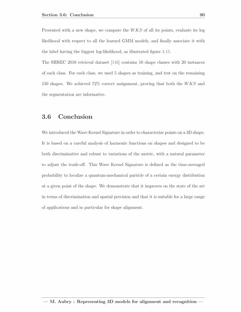
Section 3.6: Conclusion 90
Presented with a new shape, we compute the WKS of all its points, evaluate its log
likelihood with respect to all the learned GMM models, and finally associate it with
the label having the biggest log-likelihood, as illustrated figure 3.15.
The SHREC 2010 retrieval dataset [116] contains 10 shape classes with 20 instances
of each class. For each class, we used 5 shapes as training, and test on the remaining
150 shapes. We achieved 72% correct assignment, proving that both the WKS and
the segmentation are informative.
3.6 Conclusion
We introduced the Wave Kernel Signature in order to characterize points on a 3D shape.
It is based on a careful analysis of harmonic functions on shapes and designed to be
both discriminative and robust to variations of the metric, with a natural parameter
to adjust the trade-off. This Wave Kernel Signature is defined as the time-averaged
probability to localize a quantum-mechanical particle of a certain energy distribution
at a given point of the shape. We demonstrate that it improves on the state of the art
in terms of discrimination and spatial precision and that it is suitable for a large range
of applications and in particular for shape alignment.
— M. Aubry : Representing 3D models for alignment and recognition —

91
Chapter 4
Painting-to-3D Alignment
4.1 Introduction
In the previous chapter, we tackled the problem of describing 3D models for 3D to
3D instance alignment. Here we want to develop a representation of 3D models that
enables alignments of 2D depictions to a 3D model. We go beyond what methods
reviewed in 2.2.2 and 2.2.3 can do and focus on recovering the viewpoint of historical
and non-realistic depictions of an architectural site, such as drawings, paintings and
historical photographs, with respect to a 3D model of the site. This is a tremendously
difficult task since the appearance and the scene structure in the 2D depictions can
be very different from the appearance and the geometry of the 3D model, e.g., due to
the specific rendering style, drawing error, age, lighting or change of seasons (see figure
1.4). In addition, we face a hard search problem: the number of possible alignments of
a painting to a large 3D model, such as a partial reconstruction of a city, is huge. To
address these issues, we develop a new compact representation of complex 3D scenes.
The 3D model of the scene is represented by a set of 3D discriminative visual elements
that are automatically learnt from rendered views. Similar to object detection, the set
— M. Aubry : Representing 3D models for alignment and recognition —

Section 4.1: Introduction 92
(a) Internet paintings and drawings. (b) 3D model.
(c) Aligned painting to 3D model. (d) Alignment results visualized in Google Earth.
Figure 4.1: Our system automatically recovers the viewpoint of paintings, drawings,and historical photographs with respect to a 3D model of an architectural site. Paintingin (c) courtesy of Podi Lawrence.
of visual elements, as well as the weights of individual features for each element, are
learnt in a discriminative fashion. We show that the learnt visual elements are reliably
matched in 2D depictions of the scene despite large variations in rendering style (e.g.
watercolor, sketch, historical photograph) and structural changes (e.g. missing scene
parts, large occluders) of the scene. We demonstrate an application of the proposed
approach to automatic re-photography to find an approximate viewpoint of historical
paintings and photographs with respect to a 3D model of the site. The proposed align-
ment procedure is validated via a human user study on a new database of paintings
and sketches spanning several sites. The results demonstrate that our algorithm pro-
duces significantly better alignments than several baseline methods. Example results
are shown in figure 4.1.
— M. Aubry : Representing 3D models for alignment and recognition —

Section 4.1: Introduction 93
4.1.1 Motivation
Why is this task important? First, non-photographic depictions are plentiful and com-
prise a large portion of our visual record. We wish to reason about them, and aligning
such depictions to reference imagery (via a 3D model in this case) is an important
step towards this goal. Second, such technology would open up a number of exciting
computer graphics applications that currently require expensive manual alignment of
3D models to various forms of 2D imagery. Examples include interactive visualization
of a 3D site across time and different rendering styles [52, 113], model-based image
enhancement [105], annotation transfer for augmented reality [165], inverse procedu-
ral 3D modeling [7, 130] or computational re-photography [25, 141]. Finally, reliable
automatic image to 3D model matching is important in domains where reference 3D
models are often available, but may contain errors or unexpected changes (e.g. some-
thing built/destroyed) [32], such as urban planning, civil engineering or archaeology.
4.1.2 From locally invariant to discriminatively trained fea-
tures
Local feature based methods presented in 2.2.2 represent a powerful tool for match-
ing photographs of the same at least lightly textured scene despite changes in view-
point, scale, illumination, and partial occlusion. However, appearance changes beyond
the modeled invariance, such as significant perspective distortions, non-rigid deforma-
tions, non-linear illumination changes (e.g. shadows), weathering, change of seasons,
structural variations or a different depiction style (see examples figure 1.4) cause local
feature-based methods to fail [84, 147, 160], as illustrated figure 1.5.
— M. Aubry : Representing 3D models for alignment and recognition —

Section 4.1: Introduction 94
Because of these limitations of standard local features methods, we turn towards meth-
ods based on discriminative learning similar to those used for object category recogni-
tion and presented in 2.3.1.2 and 2.3.1.3. They rely on a weighted spatial distribution
of image gradient orientations. The weights are learnt in a discriminative fashion
to emphasize object contours and de-emphasize non-object, background contours and
clutter. Such a representation can capture complex object boundaries in a soft manner,
avoiding hard decisions about the presence and connectivity of imaged object edges.
Learnt weights have also been shown to emphasize visually salient image structures
matchable across different image domains, such as sketches and photographs [160].
Similar representation has been used to learn architectural elements that summarize
a certain geo-spatial area by analyzing (approximately rectified) 2D street-view pho-
tographs from multiple cities [55]. Also related is a contemporary work that utilizes
similar representation for scene [96] and action [93] classification.
Building on these works we develop a compact representation of 3D scenes suitable
for alignment to 2D depictions. In contrast to [55, 160] who analyze 2D images, our
method takes advantage of the knowledge and control over the 3D model to learn
a representative set of mid-level 3D scene elements robust to a certain amount of
viewpoint variation and capable of recovery of the (approximate) camera viewpoint. We
show that the learnt mid-level scene elements are reliably detectable in 2D depictions
of the scene despite large changes in appearance and rendering style.
4.1.3 Overview
In this chapter, we focus on depictions that are, at least approximately, perspective
renderings of the 3D scene and we consider complex textured 3D models obtained by
— M. Aubry : Representing 3D models for alignment and recognition —

Section 4.1: Introduction 95
Figure 4.2: Approach overview. In the offline stage (left) we summarize a given3D model as a collection of discriminative visual elements learnt from rendered views ofthe site (middle). In the online stage (right) we match the learnt visual elements to theinput painting and use the obtained correspondences to recover the camera viewpointwith respect to the 3D model.
recent multi-view stereo reconstruction systems [70] as well as simplified models ob-
tained from 3D modeling tools such as Trimble 3D Warehouse.
In section 4.2 we develop the two key ideas behind our work. First, we introduce our
representation of 3D models, 3D discriminative visual elements. Then, we explain how
to cast the problem of matching 3D discriminative visual elements to a query image as
a classification problem.
The proposed method has two stages: first, in an offline stage we learn a set of 3D
discriminative visual elements representing the architectural site; second, in an online
stage a given unseen query painting is aligned with the 3D model by matching with
the learnt visual elements. The algorithm is detailed in figure 4.2 and in section 4.3.
— M. Aubry : Representing 3D models for alignment and recognition —
Section 4.2: 3D discriminative visual elements 96
The input to the offline stage is a 3D model of an architectural site. The output is
a set of view-dependent visual element detectors able to identify specific structures of
the 3D model in various types of 2D imagery. The approach begins by rendering a
set of representative views of the 3D model. Next, a set of visual element detectors is
computed from the rendered views by identifying scene parts that are discriminative
and can be reliably detected over a range of viewpoints. During the online stage, given
an input 2D depiction, we match the learnt visual element detectors and use the top
scoring detections to recover a coarse camera viewpoint.
To evaluate our alignment procedure, we introduce a database of paintings and sketches
spanning several sites and perform a user study where human subjects are asked to
judge the goodness of the output alignments. Our results are presented in section
4.4. We compare with several baseline methods, such as SIFT on rendered views, the
coarse viewpoint retrieval step of [147], and Exemplar SVM [160], and show that our
algorithm produces more valid alignments than the baselines. Moreover, we evaluate
our matching step on the benchmark dataset of [84] and show improvement over local
symmetry features [84] and several alternative matching criteria for our system.
4.2 3D discriminative visual elements
In this section, we present the main ideas behind our 3D model representation and
its matching to 2D depictions. We first define more precisely 3D discriminative visual
elements (section 4.2.1). We then present how we match them to test depictions by
seeing the matching problem as a classification task (section 4.2.2).
— M. Aubry : Representing 3D models for alignment and recognition —

Section 4.2: 3D discriminative visual elements 97
4.2.1 Learning 3D discriminative visual elements
We define a discriminative visual elements of a 3D scene to be a mid-level patch that is
rendered with respect to a given viewpoint from a 3D model with the following prop-
erties: (i) it is visually discriminative with respect to the rest of the “visual world”
represented here by a generic set of randomly sampled patches, (ii) it is distinctive with
respect to other patches in nearby views, and (iii) it can be reliably matched across
nearby viewpoints. We employ modern representations and recent methods for dis-
criminative learning of visual appearance, which have been successfully used in recent
object recognition systems. Our method can be viewed as “multi-view geometry [83]
meets part-based object recognition [61]” – here we wish to automatically discover the
distinctive object parts for a large 3D site.
We discover discriminative visual elements by first sampling candidate mid-level patches
across different rendered views of the 3D model. We cast the image matching problem
as a classification task over appearance features with the candidate mid-level patch as
a single positive example and a negative set consisting of a large set of “background”
patches. Note that a similar idea has been used in learning per-exemplar distances [68]
or per-exemplar support vector machine (SVM) classifiers [123] for object recogni-
tion and cross-domain image retrieval [160]. Here we apply per-exemplar learning for
matching mid-level structures between images. For a candidate mid-level patch to be
considered a discriminative visual element, we require that (i) it has a low training
error when learning the matching classifier, and (ii) it is reliably detectable in nearby
views via cross-validation.
The output for each discriminative visual element is a trained classifier. At run-time,
— M. Aubry : Representing 3D models for alignment and recognition —

Section 4.2: 3D discriminative visual elements 98
for an input painting, we run the set of trained classifiers in a sliding-window fash-
ion across different scales. Detections with high responses are considered as putative
correspondences with the 3D model, from which camera resectioning is performed.
4.2.2 Matching as classification
We formulate the matching problem as a classification task. Concretely, we want to
match a given rectangular image patch q in a rendered view (represented by a descriptor
such as HOG [49]) to its corresponding image patch in the painting, as illustrated in
figure 4.3. Instead of finding the best match measured by the Euclidean distance
between the descriptors, we train a linear classifier with q as a single positive example
(with label yq = +1) and a large number of negative examples xi for i =1 to N (with
labels yi = −1). The matching is then performed by finding the patch x∗ in the painting
with the highest classification score
s(x) = wx+ b, (4.1)
where w and b are the parameters of the linear classifier. Note that w denotes the
normal vector to the decision hyper-plane and b is a scalar offset. Compared to the
Euclidean distance, the classification score (4.1) measures a form of similarity, i.e. a
higher classification score indicates higher similarity between x and q. In addition, the
learnt w weights the components of x differently. This is in contrast to the standard
Euclidean distance where all components of x have the same weight. Parameters w
and b are obtained by minimizing a cost function of the following form
E (w, b) = L(1, wT q + b
)+
1
N
N∑i=1
L(−1, wTxi + b
), (4.2)
— M. Aubry : Representing 3D models for alignment and recognition —

Section 4.2: 3D discriminative visual elements 99
Figure 4.3: Matching as classification. Given a region and its HOG descriptor qin a rendered view (top left) the aim is to find the corresponding region in a painting(top right). This is achieved by training a linear HOG-based sliding window classifierusing q as a single positive example and a large number of negative data. The classifierweight vector w is visualized by separately showing the positive (+) and negative (-)weights at different orientations and spatial locations. The best match x in the paintingis found as the maximum of the classification score.
where the first term measures the loss L on the positive example q (also called “ex-
emplar”) and the second term measures the loss on the negative data. Note that for
simplicity we ignore in (4.2) the regularization term ||w||2, but the regularizer can be
easily added in a similar manner to [24, 73]. A particular case of the exemplar based
classifier is the exemplar-SVM [123, 160], where the loss L(y, s(x)) between the la-
bel y and predicted score s(x) is the hinge-loss L(y, s(x)) = max{0, 1 − ys(x)} [30].
For exemplar-SVM cost (4.2) is convex and can be minimized using iterative algo-
rithms [59, 156].
— M. Aubry : Representing 3D models for alignment and recognition —

Section 4.3: Discriminative visual elements for painting-to-3D alignment100
Figure 4.4: Example sampled viewpoints. Camera positions are sampled on theground plane on a regular 100×100 grid. 24 camera orientations are used for eachviewpoint. Cameras not viewing any portion of the 3D model are discarded. Thisprocedure results in about 45,000 valid views for the depicted 3D model.
4.3 Discriminative visual elements for painting-to-
3D alignment
We seek to identify elements of the 3D model that are reliably detectable in arbitrary 2D
depictions. As explained in section 4.2, we build on discriminative learning techniques
to identify visually distinctive mid-level scene structures in rendered views of the 3D
model . In this section, following the steps described in figure 4.2, we specify the design
choices we made to solve our specific problem of matching a painting to the 3D model
of an architectural site.
4.3.1 View selection and representation
The aim is to extract from the 3D model a set of view-dependent 2D descriptors suit-
able for alignment to 2D depictions. This is achieved by sampling representative views
of the 3D model and learning visual element detectors from the rendered appearance
in the sampled views. We sample possible views of the 3D model in a similar manner
to [22, 90, 147]. First, we identify the ground plane and corresponding vertical direc-
— M. Aubry : Representing 3D models for alignment and recognition —

Section 4.3: Discriminative visual elements for painting-to-3D alignment101
tion. The camera positions are then sampled on the ground plane on a regular grid.
For each camera position we sample 12 possible horizontal camera rotations assuming
no in-plane rotation of the camera. For each horizontal rotation we sample 2 vertical
rotations (pitch angles). Views where less than 5% of the pixels are occupied by the 3D
model are discarded. This procedure results in 7,000-45,000 views depending on the
size of the 3D site. Example sampled camera positions are shown in figure 4.4. Note
that the rendered views form only an intermediate representation and can be discarded
after visual element detectors are extracted. We render views from the 3D model by
adapting the publicly available OpenGL code from [147] to work with our models. The
renderer simply ray casts and samples colors from the textured models against a white
background, and does not explicitly reason about illumination effects, such as shadows
or specularities (although the textured models may implicitly include this information).
Each rendered view is represented by densely sampled patches at multiple scales, with
each patch represented by a Histogram of Oriented Gradient (HOG) descriptor [49] (see
section 2.3.1.2 for a review of HOG). We use the publicly available implementation of
HOG from [61]. We only use the contrast insensitive portion of the HOG descriptor
on a 10 x 10 grid of cells with 9 orientations within each cell, which results in an
900 dimensional descriptor. The HOG descriptor is forgiving to small drawing errors
thanks to its spatial and orientation binning. In addition, we use a contrast insensitive
HOG to enhance the capability of matching across different depiction styles.
— M. Aubry : Representing 3D models for alignment and recognition —

Section 4.3: Discriminative visual elements for painting-to-3D alignment102
4.3.2 Least squares model for visual element selection and
matching
Every rendered view has thousands of potential visual elements and the task is to
identify those that are distinct and hence likely to be detectable in different depictions.
For example, a specific tower on the building may be distinctive for the site, whereas
a patch in the middle of a gray wall may not. In the following, we show that using
a least squares loss function, the classifier can be computed in closed-form without
computationally expensive iterative training. In turn, this enables efficient training of
candidate visual element detectors corresponding to image patches that are densely
sampled in each rendered view. The quality of the trained detector (measured by
the training error) is then used to select only the few candidate visual elements that
are the most discriminative in each view (have the lowest training error). Finally, we
show how the learnt visual elements are matched to the input painting, and relate the
proposed approach to other recent work on closed-form training of HOG-based linear
classifiers [73, 81].
4.3.2.1 Selection of discriminative visual elements via least squares regres-
sion
In section 4.2.2 we have assumed that the position and scale of the visual element q
in the rendered view was given. As storing and matching all possible visual elements
from all rendered views would be computationally prohibitive, the aim here is to auto-
matically select a subset of the visual elements that are the most discriminative. First,
we note that the optimal value of the cost (4.2) characterizes the separability of a par-
ticular candidate visual element q from the (fixed) negative examples {xi} and hence
— M. Aubry : Representing 3D models for alignment and recognition —

Section 4.3: Discriminative visual elements for painting-to-3D alignment103
can be used for measuring the degree of discriminability of q. However, when using
a hinge-loss as in exemplar SVM, optimizing (4.2) would be expensive to perform for
thousands of candidate elements in each rendered view. Instead, similarly to [24, 73],
we take advantage of the fact that in the case of square loss L(y, s(x)) = (y − s(x))2
the wLS and bLS minimizing (4.2) and the optimal cost E∗LS can be obtained in closed
form as
wLS =2
2 + ‖Φ(q)‖2Σ−1(q − μ), (4.3)
bLS = −1
2(q + μ)TwLS, (4.4)
E∗LS =
4
2 + ‖Φ(q)‖2 , (4.5)
where μ = 1N
∑Ni=1 xi denotes the mean of the negative examples, Σ = 1
N
∑Ni=1(xi −
μ)(xi − μ) their covariance and
‖Φ(q)‖2 = (q − μ)Σ−1(q − μ), (4.6)
the squared norm of q after the “whitening” transformation
Φ(q) = Σ− 12 (q − μ). (4.7)
We can use the value of the optimal cost (4.5) as a measure of the discriminability of a
specific q. If the training cost (error) for a specific candidate visual element q is small
the element is discriminative. If the training cost is large the candidate visual element
q is not discriminative. This observation can be translated into a simple and efficient
— M. Aubry : Representing 3D models for alignment and recognition —

Section 4.3: Discriminative visual elements for painting-to-3D alignment104
Figure 4.5: Selection of discriminative visual elements. First row: discrim-inability scores shown as a heat-map for three different scales. Red indicates highdiscriminability. Blue indicates low discriminability. The discriminability is inverselyproportional to the training cost of a classifier learnt from a patch at the particularimage location. Second row: example visual elements at the local maxima of the dis-criminability scores. The corresponding local maxima are also indicated using “x” inthe heat-maps above.
algorithm for ranking candidate element detectors based on their discriminability. In
practice, we evaluate the squared “whitened” norm ‖Φ(q)‖2 of each candidate element
q, which is inversely proportional to the training cost. If the whitened norm is high the
candidate element is discriminative, if the whitened norm is low the candidate element
is not discriminative. Given a rendered view, we consider as candidates visual element
detectors of all patches that are local maxima (in scale and space) of the norm of their
whitened HOG descriptor, ‖Φ(q)‖2. Non-maximum suppression is performed using
a threshold of 0.1 on the standard ratio of area intersection over union between two
neighboring patches. Illustration of multi-scale discriminative visual element selection
for an example rendered view is shown in figure 4.5.
— M. Aubry : Representing 3D models for alignment and recognition —

Section 4.3: Discriminative visual elements for painting-to-3D alignment105
4.3.2.2 Relation to linear discriminant analysis (LDA)
Recent works [73, 81] have shown that linear HOG-based object detectors computed
analytically using linear discriminant analysis (LDA) can reach similar object detection
accuracy as detectors learnt by expensive iterative SVM training. The distribution of
positive and negative data points is assumed to be Gaussian, with mean vectors μp
and μn, respectively. The covariance matrix Σp = Σn = Σ is assumed to be the
same for both positive and negative data. Under these Gaussian assumptions, the
decision hyperplane can be obtained via a ratio test in closed form. Applying this
approach to our image matching set-up, we estimate μn and Σ from a large set of
HOG descriptors extracted from patches that are sampled from a set of (“negative”)
photographs independent from all sites considered in this work. μp is set to be a
specific single HOG descriptor q of the particular positive example patch in the given
rendered view. Parameters wLDA and bLDA of the linear classifier defining the matching
score (4.1)
sLDA(x) = wTLDAx+ bLDA, (4.8)
can be obtained in closed form as
wLDA = Σ−1(q − μn), (4.9)
and
bLDA =1
2
(μTΣ−1μ− qTΣ−1q
). (4.10)
— M. Aubry : Representing 3D models for alignment and recognition —

Section 4.3: Discriminative visual elements for painting-to-3D alignment106
Figure 4.6: Selection of discriminative visual elements - interpretation usinglinear discriminant analysis. Left: The negative data distribution (centered at μ)and two example positive data distributions (q1 and q2) are modeled as Gaussians withdifferent means but the same covariance. Right: After “whitening”, the negative datais centered at the origin with unit covariance. For fixed negative data, the classifierdefined by q2 is clearly more discriminative than the classifier defined by q1, as measuredby the overlap of the positive and negative data distributions. In the whitened space,this overlap can be measured by the Euclidean distance of the (whitened) mean of thepositive data points from the origin. Note that in the original non-whitened space (left)the means of q1 and q2 are at the same distance from the mean of the negative data μ.
Note that the matching score (4.8) can also be expressed using the whitening transfor-
mation defined in (4.7) as
sLDA(x) = Φ(q)TΦ(x)− 1
2‖Φ(q)‖2, (4.11)
where the first term is a dot-product between whitened q and x, and the second term
is an additive normalization factor reducing the matching score for q vectors with
large whitened norm. It is interesting to note that under the Gaussian assumptions
of LDA, the squared whitened norm ‖Φ(q)‖2 can be interpreted as the Bhattacharyya
distance [98] measuring the “overlap” between the Gaussian representing the negative
data and the Gaussian representing the positive example q. Discriminative visual
elements q with large ‖Φ(q)‖ (as described in section 4.3.2.1) correspond to “unusual”
examples far from the distribution of the negative data. This intuition is illustrated in
figure 4.6.
— M. Aubry : Representing 3D models for alignment and recognition —

Section 4.3: Discriminative visual elements for painting-to-3D alignment107
4.3.2.3 Discussion
Classifiers obtained by minimizing the least squares cost function (4.2) or satisfying
the LDA ratio test can be used for matching a candidate visual element q to a painting
as described in equation (4.1). Note that the decision hyperplanes obtained from the
least squares regression, wLS, and linear discriminant analysis, wLDA, are parallel. As
a consequence, for a particular visual element q the ranking of matches according to
the matching score (4.1) would be identical for the two methods. In other words, in an
object detection set-up [49, 73, 81] the two methods would produce identical precision-
recall curves. In our matching set-up, for a given q the best match in a particular
painting would be identical for both methods. The actual value of the score, however,
becomes important when comparing matching scores across different visual element
detectors q. In object detection, the score of the learnt classifiers is typically calibrated
on a held-out set of labeled validation examples [123].
4.3.3 Calibrated discriminative matching
We have found that calibration of matching scores across different visual elements is
important for the quality of the final matching results. Below we describe a procedure
to calibrate matching scores without the need of any labelled data. First, we found
(section 4.4.4.3) that the matching score obtained from LDA produces significantly
better matching results than matching via least squares regression. Nevertheless, we
found that the raw uncalibrated LDA score favors low-contrast image regions, which
have an almost zero HOG descriptor. To avoid this problem, we further calibrate the
LDA score (4.8) by subtracting a term that measures the score of the visual element q
— M. Aubry : Representing 3D models for alignment and recognition —

Section 4.3: Discriminative visual elements for painting-to-3D alignment108
matched to a low-contrast region, represented by zero (empty) HOG vector
scalib(x) = sLDA(x)− sLDA(0) (4.12)
= (q − μ)TΣ−1x. (4.13)
This calibrated score gives much better results on the dataset of [84] as shown in
section 4.4.4.3 and significantly improves matching results on our dataset of historical
photographs and non-photographic depictions.
4.3.4 Filtering elements unstable across viewpoint
Here we wish to discard elements that cannot be reliably detected in close-by rendered
views. This filtering criterion removes many unstable elements that are, for example,
ambiguous because of repeated structures in the rendered view or cover large depth
discontinuities and hence significantly change with viewpoint.
We define close-by views based on the visual overlap of imaged 3D structures rather
than, for example, the distance between camera centers. In detail, to measure visual
overlap between views V 1, V 2 we define the following score
S(V 1, V 2) =1
|V|∑
{x1i ,x
2i }∈V
e− (x1i−x2i )
2
2σ2x
− 1
2σ2d
(d(x1i )−d(x2i ))2
12 (d(x1
i)+d(x2
i))2 , (4.14)
where {x1i , x2i } ∈ V is the set of corresponding points (pixels) in view V 1 and V 2,
respectively, xji is the location of pixel i in view j, d(xji ) is the depth (distance to
the 3D model) at pixel i in view j, and σx and σd are parameters. The first term in
the exponent measures the squared image distance between the corresponding pixels.
— M. Aubry : Representing 3D models for alignment and recognition —

Section 4.3: Discriminative visual elements for painting-to-3D alignment109
(a) Top 4 stable patches (b) Top 4 unstable patches
Figure 4.7: Filtering elements unstable across viewpoint. Examples of topstable (left) and unstable (right) visual elements detected in one of the rendered views.Unstable elements are typically detected on repeated structures or occlusion boundariesand are removed.
The second term in the exponent measures the difference between the depths at the
corresponding pixel locations normalized by their average depth. The per-pixel scores
are then averaged over all corresponding pixels in the two views. The score is one
if the two views are identical and zero if the two views have no visual overlap. In
our case, two views are deemed “close-by” if their visual overlap score is greater than
0.4. Note that the score depends on camera positions as well as the 3D structure as
it measures differences between projected 3D points in the image plane. As a result,
the score is, for example, less sensitive to small camera translations if the camera is
looking at a far away scene. We found that good values for the parameters are σd = 0.3
and σx = (W +H)/10, where W and H are, respectively, the width and height of the
rendered views.
Here we evaluate if each candidate discriminative visual element obtained as described
in section 4.3.2 is stable. Equipped with the above definition of nearby views, we test if
each candidate visual element can be correctly detected in the set of nearby views using
the ground truth locations of the candidate element obtained from the knowledge of
the 3D model. In detail, we first select the near-by views in which the visual element is
fully visible. Then, we attempt to localize the visual element in each view by applying
— M. Aubry : Representing 3D models for alignment and recognition —

Section 4.3: Discriminative visual elements for painting-to-3D alignment110
Figure 4.8: Examples of selected visual elements for a 3D site. Top: Selectionof top ranked 50 visual elements visible from this specific view of the site. Each elementis depicted as a planar patch with an orientation of the plane parallel to the cameraplane of its corresponding source view. Bottom: Subset of 9 elements shown fromtheir original viewpoints. Note that the proposed algorithm prefers visually salientscene structures such as the two towers in the top-right or the building in the left partof the view. In contrast, some repetitive and non-salient scene structures in the rightportion of the picture are ignored.
the corresponding linear detector given by eq. (4.12) in a sliding window fashion. To
suppress potential repeated structures, we require that the ratio between the score of
the first and second highest scoring detection in the image is larger than a threshold of
1.04, similar to [121]. We keep visual elements that are successfully detected in more
than 80% of the nearby views. Examples of stable and unstable visual elements are
shown in figure 4.7.
This procedure typically results in several thousand selected elements for each archi-
tectural site. Examples of the final visual elements obtained by the proposed approach
are shown in figure 4.8.
— M. Aubry : Representing 3D models for alignment and recognition —
Section 4.3: Discriminative visual elements for painting-to-3D alignment111
4.3.5 Robust matching
Since we wish to obtain matches that are both (i) non-ambiguous and (ii) have a high
matching score we perform the following two step procedure to select candidates visual
element matches for a given depiction. First, we apply all visual element detectors
densely and at all scales on the depiction using the calibrated similarity score (4.12),
perform non-max suppression and take the top 200 detections sorted according to
the first to second nearest neighbor ratio [121]. This selects the most non-ambiguous
matches. Second, we sort the 200 matches directly by score (4.12) and consider the
top 25 matches to compute the camera viewpoint as described in section 4.3.6.
4.3.6 Recovering viewpoint
In this section we describe how, given the set of discriminative visual elements gleaned
from the 3D model, to recover the viewpoint and intrinsic parameters of an input
painting or historical photograph with respect to the 3D model. We assume that the
paintings are perspective scene renderings and seek to recover the camera center and
rotation via camera resectioning [83].
For detection, each discriminative visual element takes as input a 2D patch from the
painting and returns as output a 3D location X on the 3D model, a plane represent-
ing the patch extent on the 3D model centered at X, and a detector response score
indicating the quality of the appearance match. Following the matching procedure
described in section 4.3.3, we form a set of 25 putative discriminative visual element
matches. From each putative visual element match we obtain 5 putative point cor-
respondences by taking the 2D/3D locations of the patch center and its four corners.
The patch corners provide information about the patch scale and the planar location
— M. Aubry : Representing 3D models for alignment and recognition —
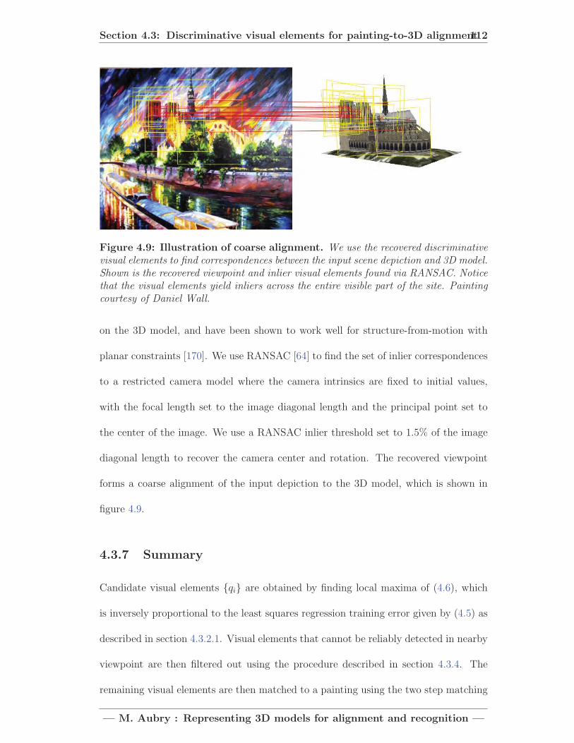
Section 4.3: Discriminative visual elements for painting-to-3D alignment112
Figure 4.9: Illustration of coarse alignment. We use the recovered discriminativevisual elements to find correspondences between the input scene depiction and 3D model.Shown is the recovered viewpoint and inlier visual elements found via RANSAC. Noticethat the visual elements yield inliers across the entire visible part of the site. Paintingcourtesy of Daniel Wall.
on the 3D model, and have been shown to work well for structure-from-motion with
planar constraints [170]. We use RANSAC [64] to find the set of inlier correspondences
to a restricted camera model where the camera intrinsics are fixed to initial values,
with the focal length set to the image diagonal length and the principal point set to
the center of the image. We use a RANSAC inlier threshold set to 1.5% of the image
diagonal length to recover the camera center and rotation. The recovered viewpoint
forms a coarse alignment of the input depiction to the 3D model, which is shown in
figure 4.9.
4.3.7 Summary
Candidate visual elements {qi} are obtained by finding local maxima of (4.6), which
is inversely proportional to the least squares regression training error given by (4.5) as
described in section 4.3.2.1. Visual elements that cannot be reliably detected in nearby
viewpoint are then filtered out using the procedure described in section 4.3.4. The
remaining visual elements are then matched to a painting using the two step matching
— M. Aubry : Representing 3D models for alignment and recognition —

Section 4.4: Results and validation 113
procedure described in section 4.3.5 that uses the calibrated LDA score (4.12). The
most confident matches are then used to recover the approximate viewpoint of the
artist with the algorithm described in section 4.3.6.
4.4 Results and validation
In this section, we first describe our dataset of non-photographic depictions and histor-
ical photographs in 4.4.1. We then provide qualitative (4.4.2) and quantitative (4.4.3)
results of our full pipeline. Finally, we provide a detailed analysis of our algorithm in
4.4.4.
4.4.1 Dataset for painting-to-3D alignment
We have collected a set of human-generated 3D models from Trimble 3D Warehouse for
the following architectural landmarks: Notre Dame of Paris, Trevi Fountain, and San
Marco’s Basilica. The Trimble 3D Warehouse models for these sites consist of basic
primitive shapes and have a composite texture from a set of images. In addition to the
Trimble 3D Warehouse models, we also consider a 3D model of San Marco’s Square
that was reconstructed from a set of photographs using dense multi-view stereo [69].
Note that while the latter 3D model has more accurate geometry than the Trimble 3D
Warehouse models, it is also much noisier along the model boundaries.
We have also collected from the Internet 85 historical photographs and 252 non-
photographic depictions of the sites. We separated the non-photographic depictions
into the following categories: ‘drawings’ (60 images), ‘engravings’ (45 images) and
‘paintings’ (147 images). The drawings category includes color renderings and the
paintings category includes different rendering styles, such as watercolors, oil paint-
— M. Aubry : Representing 3D models for alignment and recognition —

Section 4.4: Results and validation 114
Table 4.1: Statistics of our collected dataset of historical photographs and non-photographic depictions for the evaluated architectural landmarks. Note that the de-pictions of San Marco Basilica are also included in the set for San Marco Square, withthe total (bottom row) counting the number of unique depictions in our dataset.
S. Marco S. Marco Trevi NotreTotal
Square Basilica Fountain DameHist. photos 44 (30) 0 41 85Paintings 61 (41) 34 52 147Drawings 21 (19) 5 34 60Engravings 15 (9) 10 20 45
Total 141 (99) 49 147 337
(a) Input historical photographs.
(b) Aligned 3D models.
Figure 4.10: Alignment of historical photographs of San Marco’s Square to theirrespective 3D models. Photographs courtesy of la Mediatheque de l’architecture et dupatrimoine.
ings, and pastels. Table 4.1 shows the number of images belonging to each category
across the different sites.
4.4.2 Qualitative results
Figures 4.10 and 4.11 show example alignments of historical photographs and non-
photographic depictions, respectively. Notice that the depictions are reasonably well-
aligned, with regions on the 3D model rendered onto the corresponding location for a
given depiction. We are able to cope with a variety of viewpoints with respect to the
— M. Aubry : Representing 3D models for alignment and recognition —

Section 4.4: Results and validation 115
Figure 4.11: Example alignments of non-photographic depictions to 3D models. No-tice that we are able to align depictions rendered in different styles and having a varietyof viewpoints with respect to the 3D models. Images courtesy of Liz Steel, Fifi Flowers,Woom Lam Ng, and Noreen Wessling. More results are available at the projectwebsite http: // www. di. ens. fr/ willow/ research/ painting_ to_ 3d/
— M. Aubry : Representing 3D models for alignment and recognition —

Section 4.4: Results and validation 116
(a) Scene distortion. (b) Drawing and 3D errors. (c) Major structural differences.
Figure 4.12: Challenging examples successfully aligned by our method where the as-sumption of a perspective scene rendering is violated. Note that the drawing in (c) is acompletely different cathedral. Image in (a) courtesy of Blythe Scott and in (b) courtesyof Ginette Callaway.
(a) Notre Dame of Paris. (b) Trevi Fountain.
Figure 4.13: Trimble 3D Warehouse models and camera frusta depicting the recoveredviewpoints of the paintings.
3D model as well as different depiction styles. Our approach succeeds in recovering the
approximate viewpoint in spite of these challenging appearance changes and the varying
quality of the 3D models. In figure 4.12 we show alignments to a set of challenging
examples where the assumption of a perspective rendering is significantly violated,
but the proposed approach was still able to recover a reasonable alignment. Notice
the severe non-perspective scene distortions, drawing errors, and major architectural
differences (e.g. a part of the landmark may take a completely different shape).
Figure 4.13 shows the camera frusta for the recovered approximate painting viewpoints.
— M. Aubry : Representing 3D models for alignment and recognition —

Section 4.4: Results and validation 117
Notice that our system is able to recover viewpoints that are to the rear of the main
facade of the Notre Dame cathedral, which has not been possible in prior work [165]
due to the lack of reconstructed structure in these areas. Recovering approximate
camera viewpoints for paintings and historical photographs opens up the possibility of
large-scale automatic computational re-photography for such depictions [25]. The video
http://www.di.ens.fr/willow/research/painting_to_3d/data/ND.mp4 shows an
example of a virtual tour of an architectural site transitioning between viewpoints of
different images in 3D in a similar manner to [165], but here done for the challenging
case of historical photographs, non-photographic depictions, and only an approximate
3D model from Trimble 3D Warehouse. Many architectural sites now have 3D models
geo-located on a map, which, combined with the proposed approach, would enable
geo-locating historical photographs and non-photographic depictions [160] for, e.g.,
navigation and exploration of non-photorealistic depictions (as shown in our video or,
coarsely aligned manually, at http://www.whatwasthere.com) or in situ guided tours
of historical imagery using mobile or wearable display devices.
A first step into this direction is to use the geo-localization of the reference 3D models
to display the depictions on a 3D map, as shown in figure 4.14 where the paintings are
visualized in Google Earth.
4.4.3 Quantitative evaluation
In the following we give details of the performed user-study to evaluate the quality of the
alignments (section 4.4.3.1)), report the corresponding quantitative results across the
3D sites and depiction styles, and compare performance with several baseline methods
(section 4.4.3.2). We also provide a quantitative evaluation of our geo-localization
— M. Aubry : Representing 3D models for alignment and recognition —

Section 4.4: Results and validation 118
(a) Notre Dame
(b) San Marco’s Basilica.
(c) Trevi Fountain.
Figure 4.14: Examples of geo-localized depictions visualized in Google Earth. Notethat the proposed method allows us to visualize the specific place across time and throughthe eyes of different artists.
application (section 4.4.3.3).
4.4.3.1 Evaluating alignment
To quantitatively evaluate the goodness of our alignments, we have conducted a user
study via Amazon Mechanical Turk. The workers were asked to judge the viewpoint
similarity of the resulting alignments to their corresponding input depictions by cat-
egorizing the viewpoint similarity as either a (a) Good match, (b) Coarse match, or
(c) No match, illustrated in figure 4.15. We asked five different workers to rate the
viewpoint similarity for each depiction and we report the majority opinion.
— M. Aubry : Representing 3D models for alignment and recognition —

Section 4.4: Results and validation 119
(a) Good match (b) Coarse match (c) No mathch
Figure 4.15: Alignment evaluation criterion. We asked workers on AmazonMechanical Turk to judge the viewpoint similarity of the resulting alignment to theinput depiction. The workers were asked to categorize the viewpoint similarity into oneof three categories: (a) Good match – the two images show a roughly similar view of thebuilding; (b) Coarse match – the view may not be similar, but the building is roughlyat the same location in both images, not upside down, and corresponding building partscan be clearly identified; (c) No match – the views are completely different, e.g. upsidedown, little or no visual overlap. Image in (a) courtesy of Maral Sassouni and in (c)courtesy of la Mediatheque de l’architecture et du patrimoine.
Table 4.2: Viewpoint similarity user study of our algorithm across different sites.
Good Coarse Nomatch match match
S. Marco Square 51% 21% 28%S. Marco Basilica 45% 39% 15%Trevi Fountain 55% 20% 24%Notre Dame 65% 27% 9%Average 55% 27% 18%
4.4.3.2 Alignment quality and baseline comparisons
Table 4.2 shows the performance of our algorithm for the different 3D sites considered
in this work. As expected, the performance varies to some extent across the differ-
ent models depending on their size, quality and the difficulty of the matching task.
However, the failure (no match) rate remains consistently below 30%.
Table 4.3 shows the performance of our algorithm for different depiction styles aver-
aged across the 3D sites. Interestingly, the results are fairly consistent across different
depiction styles.
Finally, table 4.4 compares the performance of our algorithm to several baseline meth-
— M. Aubry : Representing 3D models for alignment and recognition —

Section 4.4: Results and validation 120
Table 4.3: Viewpoint similarity user study of our algorithm across different depictionstyles.
Good Coarse Nomatch match match
Historical photographs 59% 20% 21%Paintings 53% 30% 18%Drawings 52% 29% 19%Engravings 57% 26% 17%Average 55% 27% 18%
Table 4.4: Viewpoint similarity user study – comparison with baselines on the “SanMarco Square” 3D site.
Good Coarse Nomatch match match
SIFT on rendered views 40% 26% 33%Viewpoint retrieval [147] 1% 39% 60%Exemplar SVM [160] 34% 18% 48%
mid-level painting visual elements 33% 29% 38%3D discrim. visual elements (ours) 51% 21% 28%
ods for the 141 depictions of San Marco Square – the largest 3D model in our dataset
with 45K sampled viewpoints. We compare our algorithm against the following four
baselines: (i) SIFT on rendered views, (ii) viewpoint retrieval (corresponding to the
coarse alignment step of [147]), (iii) exemplar SVM [160], and (iv) mid-level painting
visual elements that, similar to [163], learns mid-level visual elements directly from
paintings, rather than the 3D model. The implementation details of each baseline are
given next.
For the SIFT on rendered views baseline we extract and match SIFT descriptors com-
puted at interest points across scale [121] over each input depiction and all rendered
views. We use orientation sensitive descriptors as we found them to be more reliable
than orientation invariant descriptors in practice. We perform geometric verification by
finding inliers to an affine homography between the input depiction and each rendered
viewpoint. Then, we take the rendered viewpoint with the most inliers and perform
camera resectioning with RANSAC using the SIFT putative matches for that view. We
— M. Aubry : Representing 3D models for alignment and recognition —

Section 4.4: Results and validation 121
return as output a rendering of the final resectioned viewpoint. Note that the matching
procedure is not standard since it is extracting descriptors from rendered views, which
accounts for viewpoint changes. In other words, the SIFT matching step does not need
to be viewpoint invariant as we are matching to a similar viewpoint from the rendered
set. This baseline is similar in spirit to matching with Viewpoint Invariant Patches
(VIP) [178], except no depth or rectification is needed for the paintings. This baseline
performs reasonably well, having 40% good alignments compared with 51% for our al-
gorithm. The good performance is largely due to alignments of historical photographs
(70% vs. 50% for our method). However, if historical photographs are removed from
the dataset, the SIFT on rendered views baseline drops to 27% good alignments, while
our algorithm still achieves 52% good alignments.
The viewpoint retrieval baseline consists of matching a global Gist descriptor [133]
extracted for each input depiction and all rendered views. The Gist descriptors are
compared using L2 distance and the view corresponding to the minimum distance is
returned. The Gist descriptor is sensitive to viewpoint, with the matching procedure
corresponding to the coarse alignment step of [147]. Our method clearly outperforms
the viewpoint retrieval baseline mainly because the sampled rendered views fail to cover
the enormous space of all possible viewpoints. Matching the global image-level Gist
descriptor would require much denser and wider sampling of views.
To reduce the viewpoint coverage issue, we explore as a baseline the exemplar-SVM
approach of [160]. For this a single exemplar SVM detector is trained for each input de-
piction and is subsequently matched across all scales and 2D locations in sliding window
fashion in the rendered views. While the performance improves over Gist matching,
nonetheless the results remain limited since the approach cannot handle partial occlu-
sions and significant deformations that are common in non-photorealistic depictions.
— M. Aubry : Representing 3D models for alignment and recognition —

Section 4.4: Results and validation 122
Moreover, the procedure is computationally expensive since an SVM detector is trained
with hard negative mining for each input painting, with the resulting detector run in
a sliding window fashion over all rendered views. In contrast, our approach learns
offline a few thousand visual element detectors that compactly summarize an entire
architectural site. At run time, only the learnt visual elements are applied to the input
depiction.
To overcome the issues with partial occlusion and significant deformations, but keeping
the idea of matching the input painting to the rendered views, we extract mid-level
visual elements directly from the input paintings without any explicit knowledge of the
3D model. In detail, we extract 25 mid-level discriminative visual elements from each
input painting using the approach presented in section 4.3.2.1. The painting visual
elements are then matched in a sliding window fashion to all rendered views. For
each rendered view inlier point correspondences are recovered via camera resectioning
with RANSAC over the maximal detector responses. The resectioned view that yields
the largest number of inliers is rendered and returned. Note that this baseline is
similar in spirit to learning mid-level patches [55, 163] from the input paintings without
the explicit knowledge of the 3D model. While this baseline further improves over
exemplar-SVM (38% vs. 48% failures), it does not outperform our method mainly
because it cannot combine visual element detections from multiple views available to
our method via the 3D model. Similar to the exemplar-SVM, an additional drawback
of this baseline is the high computational cost as visual elements from each painting
must be run densely across all rendered views.
— M. Aubry : Representing 3D models for alignment and recognition —

Section 4.4: Results and validation 123
Table 4.5: The percentage of input depictions that were assigned to the correct archi-tecture site split across different sites (rows) and depiction styles (columns). Note thatthere are no historical photographs for Trevi Fountain in the database.
Paintings Historical photograph Engravings Drawings AverageS. Marco Basilica 83% 87% 89% 94% 87%Trevi Fountain 82% - 90% 80% 84%Notre Dame 90% 88% 85% 79% 86%Average 86 % 87% 87% 84% 86%
4.4.3.3 Geo-localization
We explored the potential of our method for geo-localization of historical and non-
photographic depictions. We summarized the three Trimble Warehouse models with
15,000 discriminative visual elements each. For each input depiction, we applied all of
the 45,000 detectors corresponding to those elements, selected the 25 most confident
ones, and performed camera resectioning using RANSAC as described in section 4.3.6,
with the constraint that only elements from the same site could be counted as inliers.
Thus, our output is both a specific 3D model and a viewpoint.
We report our results on the task of identifying the 3D model of the architectural site.
Table 4.5 shows the results separately for the three different sites and across different
depiction styles. Despite the difficulty of the task due to the large variety of viewpoints
and styles, our method identified correctly the architectural site for 86% of the depic-
tions, which is much larger than the 33% chance performance, showing the potential
of our method for geo-localization.
— M. Aubry : Representing 3D models for alignment and recognition —

Section 4.4: Results and validation 124
(a) Original rendering (b) Drawing style (c) Painting style
Figure 4.16: Viewpoint rendering styles. We explored the possibility of render-ing viewpoints from the 3D model in different styles by applying style filters withinPhotoshop CS4 to the rendered views.
Table 4.6: Evaluation of different 3D model rendering styles.
Good Coarse Nomatch match match
Drawing style 61% 12% 27%Painting style 54% 18% 28%
Original rendering 65% 27% 9 %
4.4.4 Algorithm analysis
In this section we evaluate variants of the three steps of our algorithm: viewpoint
rendering style, visual element selection, and visual element matching. Finally, we
show and analyze the main failure modes.
4.4.4.1 Viewpoint rendering style
Since our goal is to align a 3D model to non-photorealistic depictions, we explored the
possibility of applying different rendering styles during the viewpoint rendering step of
our algorithm. We applied the ‘watercolor’ and ‘accentuated edges’ style filters from
Photoshop CS4 to our rendered views to generate, respectively, a ‘painting like’ and
a ‘drawing like’ style. Example filter outputs are shown in figure 4.16. We quantita-
tively evaluate the output of our full system (using the style filters during rendering)
on 147 depictions of the Notre Dame site via a user study on Amazon Mechanical
— M. Aubry : Representing 3D models for alignment and recognition —

Section 4.4: Results and validation 125
Figure 4.17: Evaluation of visual element selection. The average percentage(left) and number (right) of correct matches as a function of the top n matches. Seetext for details.
Turk. Results are summarized in table 4.6. Both styles result in a decrease of the
overall matching performance compared to the original rendering. However, when re-
sults are split by depiction (not reported in table 4.6) the drawing style results in a
small increase of matching performance on drawings (68% good matches vs. 62% good
matches with the original rendering). While this difference amounts to only 3 addi-
tional matched depictions, it opens-up the possibility of learning a vocabulary of visual
elements specific for each rendering style.
4.4.4.2 Visual element selection
Here we evaluate benefits of the proposed discriminative visual element selection. To
measure the improvement in the quality of the selected visual elements we compute
the percentage of correct matches (inliers). We consider only the San Marco square
3D model and the ground truth is obtained by visual inspection of the resulting align-
ments – only correct matches from the good and ok alignments are considered as
ground truth inliers. The percentage of inliers gives a finer indication of the quality
of visual elements than the overall percentage of correct alignments measured in the
— M. Aubry : Representing 3D models for alignment and recognition —

Section 4.4: Results and validation 126
Table 4.7: Evaluation of visual element matching. We report the mean averageprecision on the “desceval” task from the benchmark dataset of [84].
Matching method mAP (“desceval”)Local symmetry [84] 0.58
Least squares regression (Sec. 4.3.2.1) 0.52LDA (Sec. 4.3.2.2) 0.60Ours (Sec. 4.3.3) 0.77
previous section as RANSAC will often find the correct alignment even from very few
correct candidate correspondences. Results are summarized in figure 4.17. Here 10K
discriminative visual elements were learnt from 45K sampled views. We compare three
methods for selecting visual elements from the set of rendered views: The “3D over-
lap” (red) method selects visual elements that significantly overlap the 3D model in
rendered views, i.e. where at least 50% of the HOG support is occupied by the 3D
model. 10K visual elements are then chosen randomly out of all visual elements that
satisfy the 3D model overlap criterion. The “discriminative” (blue) method uses the
discriminative selection (section 4.3.2.1), but no cross-validation. The “discr. + X-
val” (green) uses the proposed discriminative visual element selection (section 4.3.2.1)
with cross-validation (section 4.3.3). For example, inspecting figure 4.17(a) reveals
that within the top 10 matches there are 27.9% of correct matches for the 3D overlap
method, 31.9% for the discriminative selection, and 35.4% for the discriminative se-
lection with cross-validation. This demonstrates that visual elements selected by the
proposed method are more likely to be correctly recovered in the painting.
4.4.4.3 Visual element matching
We evaluate the proposed matching procedure on the ‘desceval’ task from the bench-
mark dataset collected in [84]. The benchmark consists of challenging imagery, such
as historical photographs and non-photographic depictions of architectural landmarks.
— M. Aubry : Representing 3D models for alignment and recognition —

Section 4.4: Results and validation 127
Pairs of images in the dataset depicting a similar viewpoint of the same landmark have
been registered by fitting a homography to manual point correspondences. The task
is to find corresponding patches in each image pair. Since the ground truth correspon-
dence between points is assumed known via the homography, a precision-recall curve
can be computed for each image pair. We report the mean average precision (mAP)
measured over all image pairs in the dataset.
Following [84] we perform matching over a grid of points in the two views, with the
grid having 25 pixel spacing. In table 4.7 we report the mAP for different visual
element matching methods for our system, along with the local symmetry feature
baseline of [84]. Our full system using the calibrated matching score (section 4.3.3)
achieves a mAP of 0.77, which significantly outperforms both the alternative visual
element matching scores obtained by least squares regression (section 4.3.2.1) and linear
discriminant analysis (LDA, section 4.3.2.2), as well as the local symmetry feature
baseline.
4.4.4.4 Failure modes
We have identified three main failure modes of our algorithm, examples of which are
shown in figure 5.14. The first is due to large-scale symmetries, for example when the
front and side facade of a building are very similar. This problem is difficult to resolve
with only local reasoning. For example, the proposed cross-validation step removes
repetitive structures visible in the same view but not at different locations of the site.
The second failure mode is due to locally confusing image structures, for example, the
vertical support structures on the cathedral in figure 5.14 (middle) are locally similar
(by their HOG descriptor) to the vertical pencil strokes on the drawing. The learnt mid-
level visual elements have a larger support than typical local invariant features (such
— M. Aubry : Representing 3D models for alignment and recognition —

Section 4.4: Results and validation 128
Figure 4.18: Example failure cases. Top: large scale symmetry. Here archesare incorrectly matched on a building with similar front and the side facades. Middle:locally confusing image structures. Here the vertical support structures on the cathedral(right) are locally similar by their HOG descriptor to the vertical pencil strokes on thedrawing (left). Bottom: Two examples of paintings with unusual viewpoints. Image inthe top row courtesy of la Mediatheque de l’architecture et du patrimoine, in the middlerow courtesy of Norman Ziff and in the bottom row left courtesy of Woom Lam Ng.
as SIFT) and hence are typically more distinctive. Nevertheless, such mismatches can
occur and in some cases are geometrically consistent with a certain view of the 3D
model. The third failure mode is when the viewpoint depicted in the painting is not
covered in the set of sampled views. This can happen for unusual viewpoints including
extreme angles, large close-ups, or cropped views.
— M. Aubry : Representing 3D models for alignment and recognition —

Section 4.5: Conclusion 129
4.4.4.5 Computational cost
The most computationally demanding part of our algorithm is the selection of dis-
criminative visual elements, which can be done offline. Our basic rendering engine
outputs between 10 to 80 views per minute depending on the 3D model, but mod-
ern GPU implementations are capable of much faster rendering speeds. Additionally,
it is possible to render the views on-demand only, without ever storing them, which
could significantly reduce the storage requirements, specially for large sites. In our
Matlab implementation, the visual element selection learning time is dominated by
cross-validation. Overall, the algorithm is able to learn about 2,000 elements per hour
using 20 cores on a cluster. Note that after the offline learning only the learnt visual
elements need to be stored. Each element is represented by an 800-dimensional weight
vector, together with the 3D location, scale and orientation of the corresponding planar
patch. During the online detection stage, matching 10,000 visual elements to a 450x360
image takes about 22 minutes. The final camera resectioning takes about 25 seconds.
Both timings are on a single 4-cores machine with our Matlab implementation.
4.5 Conclusion
We have demonstrated that automatic image to 3D model alignment is possible for
a range of non-photographic depictions and historical photographs, which represent
extremely challenging cases for current local feature matching methods. To achieve this
we have developed an approach to compactly represent a 3D model of an architectural
site by a set of visually distinct mid-level scene elements extracted from rendered views,
and have shown that they can be reliably matched to a variety of photographic and non-
photographic depictions. We have also shown an application of the proposed approach
— M. Aubry : Representing 3D models for alignment and recognition —

Section 4.5: Conclusion 130
to computational re-photography to automatically find an approximate viewpoint of
historical photographs and paintings. This work is just a step towards computational
reasoning about the content of non-photographic depictions. The developed approach
for extracting visual elements opens-up the possibility of efficient indexing for visual
search of paintings and historical photographs (e.g. via hashing of the HOG features
as in [51]), or automatic fitting of complex non-perspective models used in historical
imagery [141].
— M. Aubry : Representing 3D models for alignment and recognition —

131
Chapter 5
Seeing 3D Chairs
5.1 Introduction
In chapter 3 we have designed a 3D shape descriptor adapted to 3D instance alignment.
In chapter 4, we have introduced a representation of 3D models that enabled matching
with approximate 2D perspective rendering of the model. In this chapter we want to go
beyond instance-level alignment and perform 2D-to-3D category-level alignment. To
achieve this goal, we build on the notion of discriminative visual elements introduced
in chapter 4.
We describe an object category by utilizing large quantities of 3D CAD models that
have been made publicly available online. Using the “chair” class as a running example,
we propose an exemplar-based 3D category representation, which can explicitly model
chairs of different styles as well as the large variation in viewpoint. We develop an
approach to establish part-based correspondences between 3D CAD models and real
photographs. This is achieved by (i) representing each 3D model using a set of view-
dependent mid-level visual elements learned from synthesized views in a discriminative
fashion, (ii) carefully calibrating the individual element detectors on a common dataset
— M. Aubry : Representing 3D models for alignment and recognition —

Section 5.1: Introduction 132
(a) Input images (b) Aligned output (c) 3D chair models
Figure 5.1: Given an input image (left), our algorithm searches a database of 1,3933D chair models to detect all chairs depicted in the image. The algorithm returns a 3Dmodel matching the style of the chair and recovers its viewpoint relative to the camera(outlined in green, right). We overlay a projection of the returned 3D model onto theinput image (middle). Notice the agreement of the returned model with the depictedchair style and pose.
of negative images, and (iii) matching visual elements to the test image allowing for
small mutual deformations but preserving the viewpoint and style constraints. We
demonstrate the ability of our system to align 3D models with 2D objects in the
challenging PASCAL VOC images, which depict a wide variety of chairs in complex
scenes. Example results are shown in figure 5.1.
— M. Aubry : Representing 3D models for alignment and recognition —

Section 5.1: Introduction 133
5.1.1 Motivation
From its very beginnings [144] and up until the early nineties [129], object recogni-
tion research has been heavily geometry-centric. The central tenet of the time was
alignment1, and the act of recognition was posed as correctly aligning a 3D model of
an object with its 2D depiction in the test image [89, 122]. The parameters recov-
ered during alignment (object pose, object scale, etc.) served as the output of the
recognition process, to be used, for instance, in the perception-manipulation loop in
robotics applications. Unfortunately, the success of these 3D model-based methods was
largely limited to instance recognition tasks for objects with well-pronounced rectilinear
structures (e.g. staplers were a favorite example). As the field moved toward category
recognition and objects with more complex appearance, 3D model-based object recog-
nition has been replaced by the new 2D appearance-based methods (e.g. [49, 61, 174]).
These methods forgo 3D and operate directly on the 2D image plane (see section 2.3).
Thus, instead of a 3D model of an object, they use a large dataset of 2D views of
the object class from different viewpoints, as the model. These methods have shown
steadily improving performance on a number of challenging tasks, such as the PAS-
CAL VOC dataset [58]. However, their main drawback is that the result of a successful
recognition is typically just the name of the object that was found (e.g. “chair”) and
a bounding box to indicate its rough location within the image. While this type of
result is reasonable for tasks such as retrieval (e.g. “find all chairs in this dataset”), it
is rather unsatisfying for doing any deeper reasoning about the scene (e.g. “what’s the
pose of the chair?”, “can I sit on it?”, “what is this chair occluding?”, “how can I fold
this chair?”, etc). All these questions could be trivially answered, if only we had a 3D
1Indeed, one of the oft-told stories is that when a student asked Takeo Kanade what are the threemost important problems in computer vision, his reply was: “Alignment, alignment, alignment!”.
— M. Aubry : Representing 3D models for alignment and recognition —

Section 5.1: Introduction 134
model of the chair aligned with the image!
The work presented in this chapter aims to combine some of the benefits of the 3D
model-based instance alignment methods with the modern, appearance-based object
category tools towards getting a best-of-both-worlds object recognition engine. The
idea is to use a large library of textured 3D object models that have become pub-
licly available on the Internet to implicitly represent both the 3D shape of the object
class, as well as its view-dependent 2D appearance. Our approach can be consid-
ered as a marriage between part-based discriminative models [61] and exemplar-based
matching [123]. Like part-based models, we represent objects using a set of connected
appearance parts. But, like exemplar-based methods, we avoid explicitly training an
object model by relying on a large dataset of object instances that serve as their own
model, both in 2D as well as 3D.
We picked the “chair” category as the running example in this paper because: 1) it is
very hard even for the recent methods [61], achieving only 0.13–0.20 average precision
(AP) on PASCAL VOC [1]; 2) it is a category well-represented in the publically-
available 3D model collections (e.g. Google/Trimble 3D Warehouse), 3) chairs have
huge intra-class variation – whereas there are perhaps only hundreds of types of cars
ever made, there are thousands of different types of chairs!
5.1.2 From instance-level to category-level alignment
This work is part of an emerging trend towards reclaiming some of the early successes
in 3D recognition, and combining them with modern visual recognition tools.
Most approaches tackled the problem by extending existing approaches in image-based
recognition to incorporate explicitly a simplified 3D model of the category (see section
2.3.2)
— M. Aubry : Representing 3D models for alignment and recognition —

Section 5.1: Introduction 135
Here we take another approach and extend the 3D alignment method introduced in
the previous chapter to category alignment. We do so using a data driven approach on
a much larger scale than previous works that were typically limited to a few dozens of
3D instances. This way we avoid modeling the correspondences between the different
instances or specifying a general 3D model for the category.
5.1.3 Approach Overview
Our representation consists of a large set of 3D CAD models, which captures both the
large variety of chair styles and their different possible viewpoints. Chair detection
in new images is accomplished by finding an alignment between the 2D chair and the
most similar 3D chair model rendered at the most appropriate camera viewpoint, as
shown in Figure 5.1. Aligning photographed 2D objects with the most similar (but not
identical) computer-generated 3D model is a very hard problem. Here we address it
by representing the collection of all 3D models by more than 800,000 calibrated view-
dependent mid-level visual elements learned in a discriminative fashion from rendered
views.
At test time, all the learned visual elements are applied to the test image in parallel.
The most spatially and appearance-wise consistent alignment is found, while preserv-
ing the style and viewpoint-consistency constraints. The details of the algorithm are
described in Section 5.2.
Contributions. Posing object category detection in images as a 3D instance align-
ment problem, we: 1) develop an exemplar-based 3D category representation capturing
variations across object style and viewpoint; and 2) establish the correspondence be-
tween computer-generated 3D models and 2D photographs using a large collection of
mid-level visual elements.
— M. Aubry : Representing 3D models for alignment and recognition —

Section 5.2: Discriminative visual elements for category-level 3D-2Dalignment 136
5.2 Discriminative visual elements for category-level
3D-2D alignment
Explicitly representing and synthesizing the fine-grained style and viewpoint of the
3D object category significantly simplifies the difficult task of 2D-to-3D alignment.
Nevertheless, reliably matching a synthesized view of an object to a real photograph
is still challenging due to differences in, e.g., texture, materials, color, illumination
or geometry. Furthermore, it is well known that computer generated images have
different statistical properties than real photographs. To address these issues, in a
similar manner as in chapter 4, we cast the matching problem as a classification task,
and represent the collection of 3D models using a large set of mid-level visual elements
– linear classifiers over HOG features learnt from the rendered views in a discriminative
fashion (section 5.2.1). As each of the hundreds of thousands of visual elements is learnt
individually, calibrating their matching scores becomes a critical issue. We address
this by learning a linear calibrating function for each element on a common dataset
of negative images (section 5.2.2). Finally, we wish to be tolerant to small geometric
deformations (such as a chair with longer legs or shorter armrests). We develop a
matching procedure (section 5.2.3) that allows for small deformations in the spatial
configurations of the matched visual elements while preserving consistent viewpoint
and style.
5.2.1 Representing a 3D shape collection
Similar to section 4.3.1, we need to specify valid views to represent the 3D models.
Here, our input is not a single 3D model but a large collection of 3D models. Each of
— M. Aubry : Representing 3D models for alignment and recognition —

Section 5.2: Discriminative visual elements for category-level 3D-2Dalignment 137
Figure 5.2: We represent the “chair” category by a set of 3D models of chairs ofdifferent styles t ∈ {1, ..., T} with T = 1394. The figure shows a small set of these 3Dmodels, giving a sense of their variability.
Figure 5.3: Each 3D model is represented by a set of rendered views. We render the3D models from 62 viewpoints sampled on a sphere with two different pitch angles φand 31 different azimuth angles θ. This leads to a set of valid views covering most ofthe usual chair viewpoints. These views are indexed by o ∈ {1, ...O} with O = 62.
these 3D model corresponds to a different style t ∈ {1, ..., T} with T = 1394 (see figure
5.2 for a sample of our 3D models and section 5.3.1 for details).
As shown figure 5.3, each 3D chair model was rendered on a white background from
— M. Aubry : Representing 3D models for alignment and recognition —

Section 5.2: Discriminative visual elements for category-level 3D-2Dalignment 138
Figure 5.4: We represent the “chair” category by a set of rendered views coveringdifferent styles t ∈ {1, ..., T} and viewpoints o ∈ {1, ...O}.
31 different azimuth angles and 2 different pitch angles, leading to a set of 62 views
sampled over the upper half of the viewing sphere centered on the chair. Each image is
annotated with the chair ID, t ∈ {1, ..., T}, indicating the different style, as well as the
viewing orientation indexed by o ∈ {1, ...O}. This set of rendered views corresponds
to a representation of the “chair” category (see figure 5.4).
Following the ideas developed in section 4.2 for instance-level alignment, we represent
each view by a set of visual elements. Similar to section 4.3.2, we select for each view
the most discriminative patches that minimize the least square classification error. The
patches are also represented by a 10x10 contrast invariant HOG descriptor, and the
— M. Aubry : Representing 3D models for alignment and recognition —
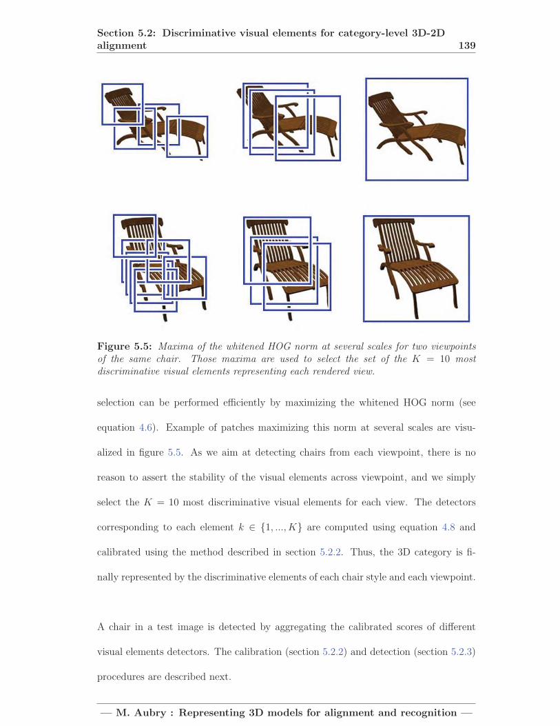
Section 5.2: Discriminative visual elements for category-level 3D-2Dalignment 139
Figure 5.5: Maxima of the whitened HOG norm at several scales for two viewpointsof the same chair. Those maxima are used to select the set of the K = 10 mostdiscriminative visual elements representing each rendered view.
selection can be performed efficiently by maximizing the whitened HOG norm (see
equation 4.6). Example of patches maximizing this norm at several scales are visu-
alized in figure 5.5. As we aim at detecting chairs from each viewpoint, there is no
reason to assert the stability of the visual elements across viewpoint, and we simply
select the K = 10 most discriminative visual elements for each view. The detectors
corresponding to each element k ∈ {1, ..., K} are computed using equation 4.8 and
calibrated using the method described in section 5.2.2. Thus, the 3D category is fi-
nally represented by the discriminative elements of each chair style and each viewpoint.
A chair in a test image is detected by aggregating the calibrated scores of different
visual elements detectors. The calibration (section 5.2.2) and detection (section 5.2.3)
procedures are described next.
— M. Aubry : Representing 3D models for alignment and recognition —

Section 5.2: Discriminative visual elements for category-level 3D-2Dalignment 140
Figure 5.6: Calibration of the different visual elements detectors. The blue curverepresent the distribution of the scores for a given classifier, and the green line thecorresponding affine calibration. A small part κ = 0.01% of the scores shown in red isassociated to positive calibrated scores.
5.2.2 Calibrating visual element detectors
As noted in prior work [123] and in section 4.3.3, calibration of matching scores across
different visual element detectors is important for the quality of the final detection
outputs. As we learn more than 800K element detectors independently, we found
careful calibration of their scores to be critical. We address this issue by running all
detectors on a common large dataset of 200K negative patches that do not contain the
object of interest. Similar to chapter 4, we represent each visual element using a linear
classifier, which scores each candidate match x as:
St,o,k(x) = wTt,o,kx (5.1)
where o is the viewpoint, t the model, k the discriminative element ID, and
wt,o,k = Σ−1(qt,o,k − μ) (5.2)
— M. Aubry : Representing 3D models for alignment and recognition —

Section 5.2: Discriminative visual elements for category-level 3D-2Dalignment 141
where qt,o,k is the HOG of the discriminative element, Σ is the covariance of the HOG
distribution and μ its mean. This detector is calibrated in an affine way:
Scalibt,o,k (x) = at,o,k St,o,k(x) + bt,o,k, (5.3)
where for each visual element detector St,o,k corresponding to the patch k of the view-
point o of the model t, we seek to find the scalars at,o,k and bt,o,k.
We recover the calibration parameters with respect to two operating points. To select
the first operating point, we run the visual element detector on 200K patches that
are randomly sampled from the negative image set, which is known to not contain
any chairs. We select as operating point the negative patch xn that yields a false
positive rate of κ. In our experiments, we used κ = 0.01%, i.e., xn is the patch
having the 99.99 percentile detection score. We choose as the second operating point
μn the mean HOG feature vector. Given these two points, we set Scalibt,o,k (xn) = 0 and
Scalibt,o,k (μn) = −1. This calibration leads to the expected false positive rate of 0.01%
when Scalibt,o,k (x) = 0. We found this to be a good compromise between representing
the tail of the score distribution and the amount of time to scan the negative data.
The calibration procedure is illustrated figure 5.6 and the influence of the calibration
parameter is analyzed in section 5.3.4.2.
5.2.3 Matching spatial configurations of visual elements
For the final object detection, we wish to enforce a consistent spatial layout of the
visual element detections corresponding to a rendered 3D view. We assume a star
model for the spatial layout, similar in spirit to [61]. The star model provides spatial
constraints, while allowing for small spatial deformations. Moreover, the star model
— M. Aubry : Representing 3D models for alignment and recognition —

Section 5.2: Discriminative visual elements for category-level 3D-2Dalignment 142
can be run in a sliding-window fashion, enabling detection of multiple object instances
in the scene.
More concretely, for all of the visual elements detectors from a single rendered 3D view
we compute a dense response map of the calibrated score (5.3) across different position
and scales of the 2D test image. For each visual element and each position in the test
image, we then replace the response by the maximum response in a 3×3 neighborhood
corresponding to the HOG cells at the same scale. This can be seen as a max pooling
of the calibrated matching scores which transforms Scalibt,o,k into Smax
t,o,k :
Smaxt,o,k (x, y, s) = max
i∈{x−1,x,x+1}max
j∈{y−1,y,y+1}Scalibt,o,k (i, j, s) (5.4)
where x, y and s are the coordinate and scale of the potential detection and i and j
cover the 3 × 3 neighborhood of (x, y). The final score Sdet(x, y, s) for a detection at
position (x, y) with scale s is the maximum among all views and chair models of the
sum of the positive scores of the different visual element matches:
Sdet(x, y, s) = maxt∈{1,...T}
maxo∈{1,..,O}
K∑k=1
max(0, Smax
t,o,k (xt,o,k, yt,o,k, st,o,k))
(5.5)
where (xt,o,k, yt,o,k, st,o,k) are the position and scale corresponding to element (t, o, k) for
a chair at position (x, y) and scale s and K is the number of discriminative elements
per rendered view. Note that we require all visual element detections to come from
the same synthesized view, which provides a strong constraint on the viewpoint and
style consistency of the detected chair. We found this matching procedure to work
well, though the view and style consistency constraints can be potentially relaxed to
accumulate matches across multiple close-by views or models with a similar style. This
part-based matching between a rendered view and an image is visualized figure 5.7
— M. Aubry : Representing 3D models for alignment and recognition —

Section 5.3: Experiments and results 143
Figure 5.7: Example of chair detection performed by our method. Each discriminativepart of a rendered view (right) is matched to the image and the scores are aggregated.Warmer color represent more confident part correspondences.
Given a match we deduce a candidate bounding box by adding 10% to the bounding
box of the aligned rendered chair. We perform non-max suppression on the resulting
bounding boxes in the following manner. Starting from the most confident detection
in the image we (i) remove all other detections that overlap this detection with more
than 0.5 area ratio overlap but only (ii) downweight (not remove) the remaining de-
tections with non-zero overlap. This procedure is then iterated starting from the next
remaining most confident detection. We found this strategy removes well overlapping
false positives while preserving highly confident (and correct) close-by detections (e.g.
chairs around a table). This motivates a system that would reason about the entire
scene jointly.
5.3 Experiments and results
In this section we introduce our new dataset of 3D chairs (section 5.3.1), show qualita-
tive output alignment results of our system (section 5.3.2) and quantitatively evaluate
our approach on images from the challenging PASCAL VOC dataset (section 5.3.3).
— M. Aubry : Representing 3D models for alignment and recognition —

Section 5.3: Experiments and results 144
Figure 5.8: Our output alignments. Parts are colored based on their detection con-fidence (warmer colors are more confident). Please see additional results on theproject webpage [4].
— M. Aubry : Representing 3D models for alignment and recognition —

Section 5.3: Experiments and results 145
We also evaluate the sensitivity of our system to several key parameters (section 5.3.4).
5.3.1 Large dataset of 3D chairs
We explicitly represent the shape variation of an object category by a large collection
of 3D CAD models. The 3D models used in this work have been downloaded from
the Google/Trimble 3D Warehouse, an on-line repository of publicly available, user-
contributed 3D graphics content created using Google SketchUp. We initially searched
the repository for “chair” and downloaded over two thousand 3D models. However,
many of them were not of good visual quality; some weren’t even chairs. After manually
culling the data, we were left with 1, 393 high-quality 3D chair models, representing a
variety of chair styles.
This dataset is our non-parametric representation of the object category explicitly
representing the large variety of chair styles. It is publicly available on the project
webpage [4].
5.3.2 Qualitative results
In Figure 5.8 we show example output alignments of our algorithm. Notice that our
algorithm can detect many different styles of chairs in different poses. For many cases,
the predicted chair matches closely the input depicted chair style and pose. In many
other cases a similar style is returned, often retrieving an accurate partial match to the
depicted chair. Moreover, our approach shows some robustness to background clutter
and partial occlusion and cropping.
In Figure 5.9 we compare the output of our algorithm with the Deformable Parts Model
(DPM) [61]. While the DPM correctly predicts the 2D location of the depicted chairs,
along with the 2D locations of its parts, our algorithm produces a more informative
— M. Aubry : Representing 3D models for alignment and recognition —

Section 5.3: Experiments and results 146
(a) Input images (b) DPM [61] output (c) Aligned outputs (d) 3D models
Figure 5.9: Comparison of our algorithm output with the deformable parts model(DPM) [61]. While the DPM correctly predicts the 2D location of the depicted chairs,along with the 2D location of its parts, our algorithm is able to predict the 3D pose andstyle of the chair.
Figure 5.10: For each image (left), we show the most confident matches (right). Evenif we do not have an exact match in our dataset, our algorithm returns reasonablematches.
result. The aligned 3D chair pose and style allows for true 3D reasoning about the
input scene.
— M. Aubry : Representing 3D models for alignment and recognition —

Section 5.3: Experiments and results 147
For a given chair detection, often there is a set of related, highly confident 3D chair
alignments having the same pose and similar style. We visualize these similar chair
alignments in Figure 5.10. Notice that the styles are similar, often sharing one or more
3D parts. This suggests that when there is not an exact style match in the database a
composite representation could be used to explain the entire input chair by composing
well-matching 3D parts from different 3D chairs. Results for the entire dataset are
available on the project webpage [4].
5.3.3 Quantitative evaluation
We evaluate the detection accuracy of our algorithm on the PASCAL VOC 2012
dataset [1]. We report detection precision-recall on images marked as non-occluded,
non-truncated, and not-difficult in the chairs validation set. While this is an easier set
compared to the full validation set, nonetheless it is very challenging due to the large
intraclass variation, chair poses, and background clutter. Note that removing these
difficult examples nonetheless yields some partially-occluded and truncated chairs, as
seen in Figure 5.8. The resulting set contains 179 images with 247 annotated chairs.
In Figure 5.11 we report full precision-recall curves for our algorithm and compare
it against two baselines: (i) DPM [61] and (ii) a root template detector using the
LDA version of Exemplar-SVM [123]. We train the root template exemplar detector
using the whitened HOG formulation described in section 4.3.2.1 assuming a single
root template that covers the entire 3D chair for the given viewpoint. We calibrate
the template as described in Section 5.2.2. During detection we run the template in a
sliding-window fashion across the input image.
Our approach achieves an average precision (AP) of 0.339 on this task. The DPM and
root template exemplar detector baselines achieve AP 0.410 and 0.055, respectively.
— M. Aubry : Representing 3D models for alignment and recognition —

Section 5.3: Experiments and results 148
0 0.2 0.4 0.6 0.8 10
0.2
0.4
0.6
0.8
1
Recall
Pre
cisi
on
Exemplar (AP: 0.055)DPM (AP: 0.410)Ours (AP: 0.339)DPM + Ours (AP: 0.452)
Figure 5.11: Precision-recall curves on PASCAL VOC 2012.
Alignment StyleGood Bad Good Ok Bad
Exemplar-LDA 52% 48% 3% 31% 66%Ours 90% 10% 21% 64% 15%
Table 5.1: Results of user study to evaluate the goodness of the alignment and stylerecovery. The data used in the user study appears on the project webpage [4].
Our performance is noteworthy as it does not use any of the PASCAL VOC training
images. We investigated combining our algorithm with DPM for the detection task.
For this we estimated an affine transformation for the DPM scores to calibrate it in the
range of our returned scores. For overlapping detected windows for the two methods,
we give one twice the confidence and discard the other. Combining our approach with
DPM yields an AP of 0.452, which significantly outperforms the DPM baseline.
We performed a user study to evaluate the quality of the output alignment and returned
chair style. For correct detections at 25% recall, users were asked to label the alignment
as “Good” (the returned alignment has very similar pose as the depicted chair) or
“Bad” (the alignment is incorrect) and to label the returned chair style as “Good” (the
returned chair style is an accurate match), “Ok” (part of the returned chair matches
— M. Aubry : Representing 3D models for alignment and recognition —

Section 5.3: Experiments and results 149
0 20 40 60 80 100 120 140 160 1800
10
20
30
40
50
60
70
Azimuth angle error (in degrees)
Perc
enta
ge o
f cha
irs a
t 25%
reca
ll
Figure 5.12: Azimuth angle error.
the depicted chair style), or “Bad” (no style match).
We report the results of the user study evaluating the quality of the returned alignments
and chair styles in Table 5.1. We compare against the root template exemplar baseline
and outperform it on both tasks. The fact that the number of exact matches is only
3% for the baseline exemplar detector suggests that there are just too many variations
within the chair category. This also motivates using a part-based approach since we
are able to obtain high quality partial matches, allowing us to find a close-by chair,
whereas the root template detector (Exemplar-LDA baseline) must match the entire
chair at once. We found that it was somewhat difficult to judge the returned styles
from the exemplar-LDA baseline since the matches were not as good.
Finally, we quantitatively evaluated the accuracy of the estimated chair orientation.
For this, we manually annotated the azimuth angle for the same set of detections as
used in the user study. Our algorithm returns an azimuth angle within 20◦ of the
ground truth for 87% of the examples. The complete distribution of the orientation
errors is shown in figure 5.12.
— M. Aubry : Representing 3D models for alignment and recognition —

Section 5.3: Experiments and results 150
Figure 5.13: Detection performance of our algorithm as a function of the number of3D models used to describe the category.
5.3.4 Algorithm analysis
In this section, we evaluate the influence of several key parameters of our algorithm,
namely the number of 3D models (section 5.3.4.1) and the calibration parameter κ (sec-
tion 5.3.4.2). We also evaluate the closed-form calibration procedure presented in the
previous chapter section 4.3.3 (section 5.3.4.2) and the benefit of using discriminative
elements instead of elements chosen on a grid (section 5.3.4.3). Finally, we discuss the
main failure cases of our method (section 5.3.4.4) and discuss its computational cost
(section 5.3.4.5). Except when specified otherwise, all the 1392 3D models are used,
the calibration parameter is κ = 10−4 and the views are used in their original rendering
(600 × 600 pixel images where the size of the chair may vary) and the minimum size
of a discriminative element is 100× 100 pixels.
5.3.4.1 Number of 3D models
Having a big collection of 3D models is important to have a good representation of
an object class. We performed the same detection experiment as the one described in
— M. Aubry : Representing 3D models for alignment and recognition —

Section 5.3: Experiments and results 151
Table 5.2: AP evolution with the number of 3D models
models 10 20 30 40 50 100 200 500 1000 1300 1392AP (%) 19.4 24.3 26.1 28.7 30.5 32.0 32.8 33.5 34.2 34.6 34.9
Table 5.3: Dependency on the calibration parameter κ
calibration parameter κ 0.0001% 0.0005% 0.001% 0.005% closed form (chapter 4)AP (%) 35.2 35.2 34.9 32.9 9.3
section 5.3.3 and reported the mean average precision as a function of the number of
3D models (randomly sampled). The results are shown figure 5.13. The corresponding
values of the Average Precision are reported table 5.2. The first observation is that
using more models consistently improves the result. The curve also seems to indicate
that the improvement is still far from convergence and that more 3D models will further
improve the performance.
5.3.4.2 Calibration
The calibration procedure we have developed in section 5.2.2 using negative data is
different from the one of section 4.3.3, which was defined in the closed form. The one
used in this chapter has two main advantages. First, it allows us to discard immediately
most of the potential matches, i.e. the 99.99% with scores lower than 0. This makes the
alignment procedure more efficient. Second, the calibration of section 4.3.3 makes the
0 score meaningful and thus the fact of considering only positive scores as in equation
(5.5) possible.
Because of the inefficiency of the detection method of chapter 4 which requires keeping
all candidate matches, we used only 100 chairs models to compare the two methods.
The MAP detection score obtained with the discriminative calibration of section 5.2.2
is 0.320, while the score with closed form calibration of chapter 4 is only 0.093, showing
a clear advantage for the method developed in this chapter.
— M. Aubry : Representing 3D models for alignment and recognition —

Section 5.3: Experiments and results 152
Table 5.4: Detection AP as a function of the visual elements size (with respect to thelarges dimension of the chair)
relative size 1.8 2.4 2.8AP (%) 27.2 25.2 17.6
Another interesting question is the choice of the calibration parameter κ. Working with
much larger or much smaller value of the calibration parameter κ is problematic for
computational reasons. If the parameter is large, we will have to consider many poten-
tial matches for the alignment. If it is small, we will have to evaluate the distribution
of the scores on a much larger set of negative examples to calibrate the detectors. We
experimented with several parameters κ and report the results in table 5.3. The detec-
tion score obtained with a calibration parameter κ = 0.001% is 0.352, which is slightly
but not significantly better than the 0.349 obtained in exactly the same conditions with
κ = 0.01%. Qualitatively, the results are also very similar using the two parameters.
This shows that the method is robust to the choice of the calibration parameter κ.
5.3.4.3 Deterministic part selection
To demonstrate the benefits of our discriminative part selection, we have defined visual
elements manually on a regular grid and tried to match them using the same framework
as before. We have overlapped a 3 by 3 grid of elements on top of the rendered views and
tested different relative size of the visual elements with respect to the larges dimension
of the chair. We have added a global element which overlaps the full chair. This leads
to a total of ten elements per rendered view which can be directly compared to the
previous results. The results for several relative size of the visual elements are reported
table 5.4. It can be seen that that defining the elements in this way strongly harms the
performance, leading to a maximum of 27% average precision (to compare with 35.2%
— M. Aubry : Representing 3D models for alignment and recognition —

Section 5.3: Experiments and results 153
(a) Confusing discriminative patterns
(b) Chair-like structures in the background
(c) Errors in pose estimation
Figure 5.14: Common failures of our algorithm.
obtained with our discriminative elements selection method).
5.3.4.4 Failure cases
In Figure 5.14 we show common failure modes of our algorithm. We observed two main
causes for false positives. First, some of the database chairs have a particular texture
that can produce confident detections on textured regions, such as the rear view of the
chair matching the checkered window pattern in Figure 5.14(a). Second, there exist
many regions in images that, through the eyes of a HOG descriptor, appear as a chair,
— M. Aubry : Representing 3D models for alignment and recognition —

Section 5.4: Conclusion 154
as seen in Figure 5.14(b). We also observed this effect in estimating the pose of the
chair, which resulted in confusing the front/back of the chair, as seen in Figure 5.14(c).
The chairs our algorithm miss are mainly special chair types, such as sofa-like chairs,
for which we do not have training examples, and chairs strongly occluded by other
objects and people.
5.3.4.5 Computational cost
Computing the discriminative elements takes 6 seconds per rendered view (1 second for
extraction and 5 seconds for calibration) on a single machine, which can be performed
offline and parallelized. The main bottleneck is having to match and align an image
to the large number of rendered views from the 3D models, which involves detecting
over 800K discriminative visual elements. Our Matlab implementation matches and
aligns an image in 2 minutes on a 80-core cluster. While this computational complexity
is high, there is room for optimism that our approach can be made significantly more
efficient. For instance, the recent part-based hashing technique of [51] could be directly
applied to our algorithm by applying winner-take-all hashing [181] on the discriminative
visual elements. As we have a similar number of part detectors as considered in their
work, we believe we can process an image in less than 20 seconds on a single multicore
processor.
5.4 Conclusion
We have demonstrated successful detection and alignment of 3D CAD chair models to
chairs depicted in 2D imagery. Our approach relied on matching spatial configurations
of mid-level discriminative visual elements extracted from a large database of CAD
— M. Aubry : Representing 3D models for alignment and recognition —

Section 5.4: Conclusion 155
models having a large number of rendered views. Our algorithm is able to recover
the chair pose, in addition to its style. We evaluated our approach on the challenging
PASCAL VOC dataset and showed that, when combined with the output of the de-
formable parts model detector [61], we are able to achieve higher detection accuracy
than using either method alone. We also demonstrated that our algorithm is able to
reliably recover the chair pose and style, as shown in our user study and orientation
error analysis. The output alignments produced by our system open up the possibility
of joint 3D reasoning about the depicted objects in a scene toward the larger goal of
full 3D scene understanding.
— M. Aubry : Representing 3D models for alignment and recognition —

156
Chapter 6
Discussion
In this chapter, we summarize the contributions of this thesis and present some future
extensions.
6.1 Contributions
In this thesis, we presented new representations of 3D models to tackle different align-
ment problems.
• in chapter 3 we have introduced the Wave Kernel Signature. It improves state
of the art results for 3D point descriptors. We have presented a mathematical
analysis of the variations of the Laplace-Beltrami eigen-values that indicates the
WKS combines the information from different spectral frequencies in an optimal
way. Beside being a natural tool for feature-based shape alignment, we have
shown that it is also well suited for many shape analysis tasks.
• in chapter 4 we have introduced the concept of 3D discriminative visual elements
to represent a 3D model in term of visual appearance. This representation is
well adapted for 2D-3D matching, and we demonstrated it can be used to align
— M. Aubry : Representing 3D models for alignment and recognition —

Section 6.2: Future work 157
(a) Isotropic diffusion.(b) Anisotropic diffusionfavoring high bending.
(c) Anisotropic diffusionfavoring low bending.
Figure 6.1: Using anisotropic instead of isotropic diffusion processes can lead to richerand more meaningful analysis of 3D shapes.
reliably non-realistic depictions to 3D models. Central to the success of our
representation is the key idea to view the feature matching problem as a least
square classification task.
• in chapter 5 we have extended the notion of discriminative visual elements to
represent not only a single 3D model but a full collection of 3D models. We have
shown that it allows to perform category-level alignment and recognition. Using
a large database of Internet CAD models and a single test image, we can predict
the position, pose and an approximate 3D model of an object.
6.2 Future work
6.2.1 Anisotropic Laplace-Beltrami operators
In chapter 3 we have worked to aggregate in an optimal way the informations from
the eigen-values and eigen-functions of the Laplace-Beltrami operator. A question
that has received little attention is to ask if the Laplace-Beltrami operator itself is an
optimal choice. Taking inspirations from works in image processing where anisotropic
diffusion is often preferable to isotropic diffusion, we introduced in [10] an anisotropic
Laplace-Beltrami operator which corresponds to anisotropic diffusion on shapes (see
— M. Aubry : Representing 3D models for alignment and recognition —

Section 6.2: Future work 158
Figure 6.2: Using parts from different 3D instances, one can explain and analyze aninstance that has never been observed.
figure 6.1). We have shown that it can improve the results of several standard shape
analysis algorithms. A more systematic study would be needed to determine how much
anisotropy can help different approaches.
6.2.2 Object compositing
In chapter 5 we have presented a method that can recover an approximate 3D model
of an object by matching it to many 3D models and selecting the most confident one.
However, this method makes little use of the fact that many 3D matches are available.
We want to explore the possibility to incorporate informations from several 3D models
to explain a given observed instance and thus predict better 3D informations from
a single image. This idea is illustrated figure 6.2 for 2D compositing. In the same
— M. Aubry : Representing 3D models for alignment and recognition —

Section 6.2: Future work 159
direction, [167] recently utilized the analysis of a large shape collection to predict
accurately the depth of a segmented 2D test instance.
6.2.3 Use of 3D shape collection analysis
In chapter 5 we have introduced a method to align shape collections with an image.
Using 3D tools similar to the one presented in chapter 3, such as the one used in
[87], to analyze automatically the 3D collection, we could transfer informations such
as parts position to an image, improving the fine grained analysis and understanding
of the image content. This exciting perspective could push new research in 3D shape
collection analysis.
6.2.4 Synthetic data for deep convolutional network training
As mentioned in section 2.3.1.4, the use of convolutional neural networks has recently
improved the performance of many vision algorithms. One of the limitation of these
networks is that they need lots of data to be trained efficiently. For example, to train a
network predicting the orientation of objects, it would be necessary to annotate a huge
database of oriented objects. To avoid this expensive manual annotation, synthetic
data could be used. However the possibility to train CNN with synthetic data remains
an open research question. In this direction, [80] recently used synthetic depth images
to train a CNN for detection from depth data.
6.2.5 Exemplar based approach with CNN features
The statistics and information encoded in CNN features is very different from the one
of more standard features. How they can be used to perform exemplar learning, similar
to what has been presented in chapter 4 for HOG descriptors is thus an open question.
— M. Aubry : Representing 3D models for alignment and recognition —

Section 6.2: Future work 160
It is however fascinating because using specifically learned features, very high quality
exemplar learning may be possible, bringing computer vision algorithms closer to what
a human is capable of doing.
— M. Aubry : Representing 3D models for alignment and recognition —

BIBLIOGRAPHY 161
Bibliography
[1] http://pascallin.ecs.soton.ac.uk/challenges/VOC/voc2012/, 2012.
[2] http://imagine.enpc.fr/ aubrym/projects/wks, 2014.
[3] http://www.di.ens.fr/willow/research/painting to 3d/, 2014.
[4] http://www.di.ens.fr/willow/research/seeing3Dchairs/, 2014.
[5] Acute 3D. http://www.acute3d.com.
[6] S. Agarwal, Y. Furukawa, N. Snavely, I. Simon, S. M. Curless, B.and Seitz, and
R. Szeliski. Building rome in a day. Communications of the ACM, 54(10):105–
112, 2011.
[7] D.G. Aliaga, P.A. Rosen, and D.R. Bekins. Style grammars for interactive visual-
ization of architecture. Visualization and Computer Graphics, IEEE Transactions
on, 13(4), 2007.
[8] B. Amberg, S. Romdhani, and T. Vetter. Optimal step nonrigid icp algorithms
for surface registration. In Proceedings of the conference on Computer Vision
and Pattern Recognition, pages 1–8, 2007.
— M. Aubry : Representing 3D models for alignment and recognition —

BIBLIOGRAPHY 162
[9] M. Andreetto, N. Brusco, and G. M. Cortelazzo. Automatic 3d modeling of
textured cultural heritage objects. Image Processing, IEEE Transactions on,
13(3):354–369, 2004.
[10] M. Andreux, E. Rodola, M. Aubry, and D. Cremers. Anisotropic laplace-beltrami
operators for shape analysis. In Sixth Workshop on Non-Rigid Shape Analysis
and Deformable Image Alignment (NORDIA), ECCV, 2014.
[11] R. Arandjelovic and A. Zisserman. Smooth object retrieval using a bag of bound-
aries. In Proceedings of International Conference on Computer Vision, pages
375–382, 2011.
[12] J. Assfalg, M. Bertini, A. Del Bimbo, and P. Pala. Content-based retrieval
of 3-d objects using spin image signatures. IEEE Transactions on Multimedia,
9(3):589–599, 2007.
[13] M. Aubry, K. Kolev, B. Goldluecke, and D. Cremers. Decoupling photometry and
geometry in dense variational camera calibration. In Proceedings of International
Conference on Computer Vision, pages 1411–1418. IEEE, 2011.
[14] M. Aubry, D. Maturana, A. A. Efros, B. C. Russell, and J. Sivic. Seeing 3d chairs:
exemplar part-based 2D-3D alignment using a large dataset of cad models. In
Proceedings of the conference on Computer Vision and Pattern Recognition, 2014.
[15] M. Aubry, S. Paris, S. Hasinoff, J. Kautz, and F. Durand. Fast local laplacian
filters: Theory and applications. ACM Transactions on Graphics, 2014.
[16] M. Aubry, S. Paris, S.W. Hasinoff, and F. Durand. Fast and robust pyramid-
based image processing. MIT technical report, 2011.
— M. Aubry : Representing 3D models for alignment and recognition —

BIBLIOGRAPHY 163
[17] M. Aubry, B. Russel, and J. Sivic. Painting-to-3d model alignment via discrimi-
native visual elements. ACM Transactions on Graphics, 2014.
[18] M. Aubry, B. Russel, and J. Sivic. Visual geo-localization of non-photographic
depictions via 2d-3d alignment. Springer, to appear in 2015.
[19] M. Aubry, B. C. Russell, and J. Sivic. Where was this picture painted?-localizing
paintings by alignment to 3d models. In Actes de la conference RFIA, 2014.
[20] M. Aubry, U. Schlickewei, and D. Cremers. Pose-consistent 3d shape segmen-
tation based on a quantum mechanical feature descriptor. Pattern Recognition,
pages 122–131, 2011.
[21] M. Aubry, U. Schlickewei, and D. Cremers. The wave kernel signature: a quantum
mechanical approach to shape analysis. In Third Workshop on 3D Representation
and Recognition (3dRR), ICCV, pages 1626–1633. IEEE, 2011.
[22] G. Baatz, O. Saurer, K. Koser, and M. Pollefeys. Large scale visual geo-
localization of images in mountainous terrain. In Proceedings of the European
Conference on Computer Vision, 2012.
[23] L. Baboud, M. Cadik, E. Eisemann, and H.-P. Seidel. Automatic photo-to-
terrain alignment for the annotation of mountain pictures. In Proceedings of the
conference on Computer Vision and Pattern Recognition, 2011.
[24] F. Bach and Z. Harchaoui. Diffrac : a discriminative and flexible framework for
clustering. In Advances in Neural Information Processing Systems, 2008.
[25] S. Bae, A. Agarwala, and F. Durand. Computational rephotography. ACM
Transactions on Graphics, 29(3), 2010.
— M. Aubry : Representing 3D models for alignment and recognition —

BIBLIOGRAPHY 164
[26] L. Ballan, G.J. Brostow, J. Puwein, and M. Pollefeys. Unstructured video-based
rendering: Interactive exploration of casually captured videos. ACM Transac-
tions on Graphics (Proc. SIGGRAPH), 2010.
[27] H. Bay, A. Ess, T. Tuytelaars, and L. Van Gool. Speeded-up robust features
(SURF). 110(3):346–359, 2008.
[28] S. Belongie, J. Malik, and J. Puzicha. Shape matching and object recognition
using shape contexts. IEEE Transactions Pattern Analysis and Machine Intelli-
gence, 24(4):509–522, 2002.
[29] P. J. Besl and N. D. McKay. Method for registration of 3-D shapes. In Robotics-
DL tentative, pages 586–606. International Society for Optics and Photonics,
1992.
[30] C. M. Bishop. Pattern Recognition and Machine Learning. Springer, 2006.
[31] A. Blake and M. Isard. Active Contours. Springer, London, 1998.
[32] F. Bosche. Automated recognition of 3D CAD model objects in laser scans and
calculation of as-built dimensions for dimensional compliance control in construc-
tion. Advanced engineering informatics, 24(1):107–118, 2010.
[33] A. Bronstein, M. Bronstein, U. Castellani, A. Dubrovina, L. Guibas, R. Horaud,
R. Kimmel, D. Knossow, E. Von Lavante, D. Mateus, et al. Shrec 2010: robust
correspondence benchmark. In Eurographics Workshop on 3D Object Retrieval
(3DOR’10), 2010.
[34] A. M. Bronstein, M. M. Bronstein, L. J. Guibas, and M. Ovsjanikov. Shape
google: Geometric words and expressions for invariant shape retrieval. ACM
Transactions on Graphics, 30(1):1, 2011.
— M. Aubry : Representing 3D models for alignment and recognition —

BIBLIOGRAPHY 165
[35] A. M. Bronstein, M. M. Bronstein, R. Kimmel, M. Mahmoudi, and G. Sapiro. A
Gromov-Hausdorff framework with diffusion geometry for topologically-robust
non-rigid shape matching. International Journal of Computer Vision, 89(2-
3):266–286, 2010.
[36] A. M. Bronstein, M. M. Bronstein, and Ron Kimmel. Efficient computation
of isometry-invariant distances between surfaces. SIAM Journal on Scientific
Computing, 28(5):1812–1836, 2006.
[37] M. M. Bronstein and I. Kokkinos. Scale-invariant heat kernel signatures for non-
rigid shape recognition. In Proceedings of the conference on Computer Vision
and Pattern Recognition, pages 1704–1711, 2010.
[38] B. J. Brown and S. Rusinkiewicz. Global non-rigid alignment of 3-D scans. In
ACM Transactions on Graphics, volume 26, page 21, 2007.
[39] M. Calonder, V. Lepetit, C. Strecha, and P. Fua. Brief: Binary robust indepen-
dent elementary features. In Proceedings of the European Conference on Com-
puter Vision, pages 778–792. 2010.
[40] J. Canny. A computational approach to edge detection. IEEE Transactions
Pattern Analysis and Machine Intelligence, (6):679–698, 1986.
[41] Y. Chen and G. Medioni. Object modelling by registration of multiple range
images. Image and vision computing, 10(3):145–155, 1992.
[42] W. Choi, Y. Chao, C. Pantofaru, and S. Savarese. Understanding indoor scenes
using 3D geometric phrases. In Proceedings of the conference on Computer Vision
and Pattern Recognition, 2013.
— M. Aubry : Representing 3D models for alignment and recognition —

BIBLIOGRAPHY 166
[43] C. S. Chua and R. Jarvis. Point signatures: A new representation for 3D object
recognition. International Journal of Computer Vision, 25(1):63–85, 1997.
[44] O. Chum and J. Matas. Geometric hashing with local affine frames. In Proceed-
ings of the conference on Computer Vision and Pattern Recognition, 2006.
[45] O. Chum, J. Philbin, J. Sivic, M. Isard, and A. Zisserman. Total Recall: Auto-
matic query expansion with a generative feature model for object retrieval. In
Proceedings of International Conference on Computer Vision, 2007.
[46] T Cox and M Cox. Multidimensional scaling. Chapman&Hall, London, UK.
[47] E. J. Crowley and A. Zisserman. In search of art. In Workshop on Computer
Vision for Art Analysis, ECCV, 2014.
[48] G. Csurka, C. Dance, L. Fan, J. Willamowski, and C. Bray. Visual categorization
with bags of keypoints. In Workshop on statistical learning in computer vision,
ECCV, volume 1, pages 1–2, 2004.
[49] N. Dalal and B. Triggs. Histograms of oriented gradients for human detection.
In Proceedings of the conference on Computer Vision and Pattern Recognition,
volume 1, pages 886–893, 2005.
[50] TOSCA dataset. http://tosca.cs.technion.ac.il/.
[51] T. Dean, M. Ruzon, M. Segal, J. Shlens, S. Vijayanarasimhan, and J. Yagnik.
Fast, accurate detection of 100,000 object classes on a single machine. In Pro-
ceedings of the conference on Computer Vision and Pattern Recognition, 2013.
[52] P. E. Debevec, C. J. Taylor, and J. Malik. Modeling and rendering architecture
from photographs. In ACM Transactions on Graphics (Proc. SIGGRAPH), 1996.
— M. Aubry : Representing 3D models for alignment and recognition —

BIBLIOGRAPHY 167
[53] L. Del Pero, J. Bowdish, B. Kermgard, E. Hartley, and K. Barnard. Understand-
ing bayesian rooms using composite 3D object models. In Proceedings of the
conference on Computer Vision and Pattern Recognition, pages 153–160, 2013.
[54] J. Deng, W. Dong, R. Socher, L.-J. Li, K. Li, and L. Fei-Fei. Imagenet: A large-
scale hierarchical image database. In Proceedings of the conference on Computer
Vision and Pattern Recognition, pages 248–255, 2009.
[55] C. Doersch, S. Singh, A. Gupta, J. Sivic, and A. A. Efros. What makes paris look
like paris? ACM Transactions on Graphics (Proc. SIGGRAPH), 31(4), 2012.
[56] Google earth. https://www.google.com/earth/.
[57] A. Elad and R. Kimmel. On bending invariant signatures for surfaces. IEEE
Transactions Pattern Analysis and Machine Intelligence, 25(10):1285–1295, 2003.
[58] M. Everingham, L. Van Gool, C. K. I. Williams, J. Winn, and A. Zisserman. The
Pascal visual object classes (VOC) challenge. International Journal of Computer
Vision, 88(2):303–338, 2010.
[59] R. Fan, K. Chang, C. Hsieh, X. Wang, and C. Lin. Liblinear: A library for
large linear classification. Journal of Machine Learning Research, 9(1):1871–
1874, 2008.
[60] O. Faugeras and R. Keriven. Complete dense stereovision using level set methods.
In Proceedings of the European Conference on Computer Vision, pages 379–393.
Springer, 1998.
[61] P. F. Felzenszwalb, R. B Girshick, D. McAllester, and D. Ramanan. Object
detection with discriminatively trained part-based models. IEEE Transactions
Pattern Analysis and Machine Intelligence, 32(9):1627–1645, 2010.
— M. Aubry : Representing 3D models for alignment and recognition —

BIBLIOGRAPHY 168
[62] Pedro F Felzenszwalb and Daniel P Huttenlocher. Pictorial structures for object
recognition. International Journal of Computer Vision, 61(1):55–79, 2005.
[63] S. Fidler, S. Dickinson, and R. Urtasun. 3d object detection and viewpoint esti-
mation with a deformable 3d cuboid model. In Advances in Neural Information
Processing Systems, pages 611–619, 2012.
[64] M. A. Fischler and R. C. Bolles. Random sample consensus: a paradigm for
model fitting with applications to image analysis and automated cartography.
Comm. of the ACM, 24(6):381–395, 1981.
[65] Martin A Fischler and Robert A Elschlager. The representation and matching
of pictorial structures. IEEE Transactions on Computers, 22(1):67–92, 1973.
[66] N. H. Fletcher and T. D. Rossing. The physics of musical instruments. Springer,
1998.
[67] W. T. Freeman and E. H. Adelson. The design and use of steerable filters. IEEE
Transactions Pattern Analysis and Machine Intelligence, 13(9):891–906, 1991.
[68] A. Frome, Y. Singer, F. Sha, and J. Malik. Learning globally-consistent local dis-
tance functions for shape-based image retrieval and classification. In Proceedings
of International Conference on Computer Vision, 2007.
[69] Y. Furukawa, B. Curless, S. M. Seitz, and R. Szeliski. Towards internet-scale
multi-view stereo. In Proceedings of the conference on Computer Vision and
Pattern Recognition, 2010.
[70] Y. Furukawa and J. Ponce. Accurate, dense, and robust multiview stereopsis.
IEEE Transactions Pattern Analysis and Machine Intelligence, 32(8):1362–1376,
2010.
— M. Aubry : Representing 3D models for alignment and recognition —

BIBLIOGRAPHY 169
[71] R. Gal, A. Shamir, and D. Cohen-Or. Pose-oblivious shape signature. IEEE
Transactions on Visualization and Computer Graphics, 13(2):261–271, 2007.
[72] N. Gelfand, N. J Mitra, L. J. Guibas, and H. Pottmann. Robust global registra-
tion. In Symposium on geometry processing, volume 2, page 5, 2005.
[73] M. Gharbi, T. Malisiewicz, S. Paris, and F. Durand. A Gaussian approximation
of feature space for fast image similarity. Technical report, MIT, 2012.
[74] G. Gilboa, N. A. Sochen, and Y. Y. Zeevi. Image enhancement and denoising by
complex diffusion processes. IEEE Transactions Pattern Analysis and Machine
Intelligence, 26(8):1020–1036, 2004.
[75] R. Girshick, J. Donahue, T. Darrell, and J. Malik. Rich feature hierarchies
for accurate object detection and semantic segmentation. Proceedings of the
conference on Computer Vision and Pattern Recognition, 2014.
[76] D. Glasner, M. Galun, S. Alpert, R. Basri, and G. Shakhnarovich. Viewpoint-
aware object detection and pose estimation. In Proceedings of International Con-
ference on Computer Vision, pages 1275–1282, 2011.
[77] B. Goldlucke, M. Aubry, K. Kolev, and D. Cremers. A super-resolution frame-
work for high-accuracy multiview reconstruction. International Journal of Com-
puter Vision, 106(2):172–191, 2014.
[78] M. Gromov. Structures metriques pour les varietes riemanniennes. Textes
Mathematiques [Mathematical Texts], 1, 1981.
[79] A. Gupta, A. A. Efros, and M. Hebert. Blocks world revisited: Image understand-
ing using qualitative geometry and mechanics. In Proceedings of the European
Conference on Computer Vision, pages 482–496. 2010.
— M. Aubry : Representing 3D models for alignment and recognition —

BIBLIOGRAPHY 170
[80] S. Gupta, R. Girshick, P. Arbelaez, and J. Malik. Learning rich features from
RGB-D images for object detection and segmentation. In Proceedings of the
European Conference on Computer Vision. 2014.
[81] B. Hariharan, J. Malik, and D. Ramanan. Discriminative decorrelation for clus-
tering and classification. In Proceedings of the European Conference on Computer
Vision, 2012.
[82] C. Harris and M. Stephens. A combined corner and edge detector. In Alvey
vision conference, volume 15, page 50. Manchester, UK, 1988.
[83] R. I. Hartley and A. Zisserman. Multiple View Geometry in Computer Vision.
Cambridge University Press, ISBN: 0521540518, second edition, 2004.
[84] D.C. Hauagge and N. Snavely. Image matching using local symmetry features.
In Proceedings of the conference on Computer Vision and Pattern Recognition,
2012.
[85] M. Hejrati and D. Ramanan. Analyzing 3d objects in cluttered images. In
Advances in Neural Information Processing Systems, pages 593–601, 2012.
[86] L. Hormander. The spectral function of an elliptic operator. Acta mathematica,
121(1):193–218, 1968.
[87] Q. Huang, F. Wang, and L. Guibas. Functional map networks for analyzing and
exploring large shape collections. ACM Transactions on Graphics, 33(4), 2014.
[88] Q.-X. Huang, B. Adams, M. Wicke, and L. J. Guibas. Non-rigid registration
under isometric deformations. volume 27, pages 1449–1457. Wiley Online Library,
2008.
— M. Aubry : Representing 3D models for alignment and recognition —
BIBLIOGRAPHY 171
[89] D. P. Huttenlocher and S. Ullman. Recognizing solid objects by alignment with
an image. International Journal of Computer Vision, 5(2):195–212, 1990.
[90] A. Irschara, C. Zach, J.-M. Frahm, and H. Bischof. From structure-from-motion
point clouds to fast location recognition. In Proceedings of the conference on
Computer Vision and Pattern Recognition, 2009.
[91] S. Izadi, D. Kim, O. Hilliges, D. Molyneaux, R. Newcombe, P. Kohli, J. Shotton,
S. Hodges, D. Freeman, A. Davison, and A. Fitzgibbon. Kinectfusion: Real-
time 3d reconstruction and interaction using a moving depth camera. In ACM
Symposium on User Interface Software and Technology, October 2011.
[92] C. L. Jackins and S. L. Tanimoto. Oct-trees and their use in representing three-
dimensional objects. Computer Graphics and Image Processing, 14(3):249–270,
1980.
[93] A. Jain, A. Gupta, M. Rodriguez, and L. S. Davis. Representing videos using
mid-level discriminative patches. In Proceedings of the conference on Computer
Vision and Pattern Recognition, 2013.
[94] A. Johnson. Spin-Images: A Representation for 3-D Surface Matching. PhD
thesis, Robotics Institute, Carnegie Mellon University, Pittsburgh, PA, August
1997.
[95] A. E. Johnson and M. Hebert. Using spin images for efficient object recogni-
tion in cluttered 3D scenes. IEEE Transactions Pattern Analysis and Machine
Intelligence, 21(5):433–449, 1999.
— M. Aubry : Representing 3D models for alignment and recognition —

BIBLIOGRAPHY 172
[96] M. Juneja, A. Vedaldi, C. V. Jawahar, and A. Zisserman. Blocks that shout:
Distinctive parts for scene classification. In Proceedings of the conference on
Computer Vision and Pattern Recognition, 2013.
[97] M. Kac. Can one hear the shape of a drum? American Mathematical Monthly,
pages 1–23, 1966.
[98] T. Kailath. The divergence and bhattacharyya distance measures in signal selec-
tion. IEEE Transactions on Communication Technology, 15(1):52–60, 1967.
[99] Y. Ke and R. Sukthankar. Pca-sift: A more distinctive representation for local
image descriptors. In Proceedings of the conference on Computer Vision and
Pattern Recognition, volume 2, pages II–506, 2004.
[100] N. Kholgade, T. Simon, A. Efros, and Y. Sheikh. 3d object manipulation in
a single photograph using stock 3d models. ACM Transactions on Computer
Graphics, 33(4), 2014.
[101] V. G. Kim, Y. Lipman, and T. Funkhouser. Blended intrinsic maps. In ACM
Transactions on Graphics, volume 30, page 79, 2011.
[102] O. Kin-Chung Au, C.-L. Tai, D. Cohen-Or, Y. Zheng, and H. Fu. Electors voting
for fast automatic shape correspondence. volume 29, pages 645–654. Wiley Online
Library, 2010.
[103] I. Kokkinos, M. M. Bronstein, R. Litman, and A. M. Bronstein. Intrinsic shape
context descriptors for deformable shapes. In Proceedings of the conference on
Computer Vision and Pattern Recognition, pages 159–166, 2012.
— M. Aubry : Representing 3D models for alignment and recognition —

BIBLIOGRAPHY 173
[104] K. Kolev, P. Tanskanen, P. Speciale, and M. Pollefeys. Turning mobile phones
into 3D scanners. In Proceedings of the conference on Computer Vision and
Pattern Recognition, 2014.
[105] J. Kopf, B. Neubert, B. Chen, M. Cohen, D. Cohen-Or, O. Deussen, M. Uyt-
tendaele, and D. Lischinski. Deep photo: Model-based photograph enhancement
and viewing. ACM Transactions on Graphics, 27(5), 2008.
[106] M. Kortgen, G.-J. Park, M. Novotni, and R. Klein. 3d shape matching with
3d shape contexts. In The 7th central European seminar on computer graphics,
volume 3, pages 5–17, 2003.
[107] A. Krizhevsky, I. Sutskever, and G. E. Hinton. Imagenet classification with deep
convolutional neural networks. In Advances in Neural Information Processing
Systems, pages 1097–1105, 2012.
[108] S. Lafon. Diffusion maps and geometric harmonics. PhD thesis, Yale University,
2004.
[109] S. Lazebnik, C. Schmid, and J. Ponce. A sparse texture representation using local
affine regions. IEEE Transactions Pattern Analysis and Machine Intelligence,
27(8):1265–1278, 2005.
[110] S. Lazebnik, C. Schmid, and J. Ponce. Beyond bags of features: Spatial pyramid
matching for recognizing natural scene categories. In Proceedings of the confer-
ence on Computer Vision and Pattern Recognition, volume 2, pages 2169–2178,
2006.
— M. Aubry : Representing 3D models for alignment and recognition —

BIBLIOGRAPHY 174
[111] Y. LeCun, B. Boser, J. S. Denker, D. Henderson, R. E. Howard, W. Hubbard,
and L. D. Jackel. Backpropagation applied to handwritten zip code recognition.
Neural computation, 1(4):541–551, 1989.
[112] Y. LeCun, L. Bottou, Y. Bengio, and P. Haffner. Gradient-based learning applied
to document recognition. Proceedings of the IEEE, 86(11):2278–2324, 1998.
[113] G. Levin and P. Debevec. Rouen revisited – interactive installation, 1999.
http://acg.media.mit.edu/people/golan/rouen/.
[114] B. Levy. Laplace-Beltrami Eigenfunctions Towards an Algorithm that ”under-
stands” geometry. In Proceedings of the International Conference on Shape Mod-
eling and Applications, page 13. IEEE, 2006.
[115] Y. Li, N. Snavely, D. Huttenlocher, and P. Fua. Worldwide pose estimation using
3D point clouds. In Proceedings of the European Conference on Computer Vision,
2012.
[116] Z. Lian, A. Godil, T. Fabry, T. Furuya, J. Hermans, R. Ohbuchi, C. Shu,
D. Smeets, P. Suetens, D. Vandermeulen, et al. SHREC’10 Track: Non-rigid
3D Shape Retrieval. In Eurographics 3DOR, 2010.
[117] J. J. Lim, H. Pirsiavash, and A. Torralba. Parsing ikea objects: Fine pose
estimation. In Proceedings of International Conference on Computer Vision,
pages 2992–2999, 2013.
[118] T. Lindeberg. Feature detection with automatic scale selection. International
Journal of Computer Vision, 30(2):76–116, 1998.
[119] Y. Lipman and T. Funkhouser. Mobius voting for surface correspondence. In
ACM Transactions on Graphics, volume 28, page 72, 2009.
— M. Aubry : Representing 3D models for alignment and recognition —

BIBLIOGRAPHY 175
[120] R. Litman and A. M. Bronstein. Learning spectral descriptors for deformable
shape correspondence. IEEE Transactions Pattern Analysis and Machine Intel-
ligence, 36(1):171–180, 2014.
[121] D. Lowe. Distinctive image features from scale-invariant keypoints. International
Journal of Computer Vision, 60(2):91–110, 2004.
[122] D. G. Lowe. Three-dimensional object recognition from single two-dimensional
images. Artificial Intelligence Journal, 31(3):355–395, 1987.
[123] T. Malisiewicz, A. Gupta, and A. A. Efros. Ensemble of exemplar-svms for object
detection and beyond. In Proceedings of International Conference on Computer
Vision, 2011.
[124] J. Matas, O. Chum, M. Urban, and T. Pajdla. Robust wide-baseline stereo from
maximally stable extremal regions. Image and Vision Computing, 22(10):761–
767, 2004.
[125] F. Memoli and G. Sapiro. A theoretical and computational framework for isom-
etry invariant recognition of point cloud data. Foundations of Computational
Mathematics, 5(3):313–347, 2005.
[126] K. Mikolajczyk and C. Schmid. Scale and affine invariant interest point detectors.
International Journal of Computer Vision, 60(1):63–86, 2004.
[127] K. Mikolajczyk and C. Schmid. A performance evaluation of local descriptors.
IEEE Transactions Pattern Analysis and Machine Intelligence, 27(10):1615–
1630, 2005.
— M. Aubry : Representing 3D models for alignment and recognition —

BIBLIOGRAPHY 176
[128] K. Mikolajczyk, T. Tuytelaars, C. Schmid, A. Zisserman, J. Matas, F. Schaf-
falitzky, T. Kadir, and L. Van Gool. A comparison of affine region detectors.
International Journal of Computer Vision, 65(1-2):43–72, 2005.
[129] J. L. Mundy. Object recognition in the geometric era: A retrospective. In Toward
category-level object recognition, pages 3–28. Springer, 2006.
[130] P. Musialski, P. Wonka, D.G. Aliaga, M. Wimmer, L. van Gool, W. Purgathofer,
N.J. Mitra, M. Pauly, M. Wand, D. Ceylan, et al. A survey of urban reconstruc-
tion. In Eurographics 2012-State of the Art Reports, 2012.
[131] R. A. Newcombe, S. Lovegrove, and A. J. Davison. DTAM: Dense tracking and
mapping in real-time. In Proceedings of International Conference on Computer
Vision, 2011.
[132] T. Ojala, M. Pietikainen, and D. Harwood. A comparative study of texture
measures with classification based on feature distributions. Pattern Recognition,
29(1):51–59, 1996.
[133] A. Oliva and A. Torralba. Modeling the shape of the scene: A holistic rep-
resentation of the spatial envelope. International Journal of Computer Vision,
42(3):145–175, 2001.
[134] A. Opelt, M. Fussenegger, A. Pinz, and P. Auer. Weak hypotheses and boosting
for generic object detection and recognition. In Proceedings of the European
Conference on Computer Vision, pages 71–84. 2004.
[135] R. Osada, T. Funkhouser, B. Chazelle, and D. Dobkin. Shape distributions. ACM
Transactions on Graphics, 21(4):807–832, 2002.
— M. Aubry : Representing 3D models for alignment and recognition —

BIBLIOGRAPHY 177
[136] M. Ovsjanikov, M. Ben-Chen, J. Solomon, A. Butscher, and L. Guibas. Func-
tional maps: a flexible representation of maps between shapes. ACM Transac-
tions on Graphics, 31(4):30, 2012.
[137] M. Ovsjanikov, Q. Merigot, F. Memoli, and L. Guibas. One point isometric
matching with the heat kernel. volume 29, pages 1555–1564. Wiley Online Li-
brary, 2010.
[138] B. Pepik, M. Stark, P. Gehler, and B. Schiele. Teaching 3d geometry to de-
formable part models. In Proceedings of the conference on Computer Vision and
Pattern Recognition, pages 3362–3369, 2012.
[139] P. Perona and J. Malik. Scale-space and edge-detection. IEEE Transactions
Pattern Analysis and Machine Intelligence, 12(7):629–639, 1990.
[140] J. Philbin, O. Chum, M. Isard, J. Sivic, and A. Zisserman. Object retrieval with
large vocabularies and fast spatial matching. In Proceedings of the conference on
Computer Vision and Pattern Recognition, 2007.
[141] J.B. Rapp. A geometrical analysis of multiple viewpoint perspective in the work of
Giovanni Battista Piranesi: an application of geometric restitution of perspective.
The Journal of Architecture, 13(6), 2008.
[142] D. Raviv, M. M. Bronstein, A. M. Bronstein, and R. Kimmel. Volumetric heat
kernel signatures. In Proceedings of the ACM workshop on 3D object retrieval,
pages 39–44, 2010.
[143] F. Rellich. Storungstheorie der Spektralzerlegung. Mathematische Annalen,
113:600–619, 1937.
— M. Aubry : Representing 3D models for alignment and recognition —
BIBLIOGRAPHY 178
[144] L. G. Roberts. Machine perception of three-dimensional solids. PhD thesis,
Massachusetts Institute of Technology, 1963.
[145] E. Rodola, S. R. Bulo, and D. Cremers. Robust region detection via consensus
segmentation of deformable shapes. In Computer Graphics Forum, volume 33,
pages 97–106, 2014.
[146] F. Rothganger, S. Lazebnik, C. Schmid, and J. Ponce. 3D object modeling and
recognition using local affine-invariant image descriptors and multi-view spatial
constraints. International Journal of Computer Vision, 66(3):231–259, 2006.
[147] B. C. Russell, J. Sivic, J. Ponce, and H. Dessales. Automatic alignment of
paintings and photographs depicting a 3D scene. In IEEE Workshop on 3D
Representation for Recognition (3dRR-11), associated with ICCV, 2011.
[148] R. M. Rustamov. Laplace-beltrami eigenfunctions for deformation invariant
shape representation. In Proceedings of the fifth Eurographics symposium on
Geometry processing, pages 225–233. Eurographics Association, 2007.
[149] J. J. Sakurai. Modern Quantum Mechanics. Addison-Wesley, 1993.
[150] S. Satkin, J. Lin, and M. Hebert. Data-driven scene understanding from 3D
models. In British Machine Vision Conference, 2012.
[151] T. Sattler, B. Leibe, and L. Kobbelt. Fast image-based localization using direct
2D-to-3D matching. In Proceedings of International Conference on Computer
Vision, 2011.
[152] F. Schaffalitzky and A. Zisserman. Multi-view matching for unordered image
sets, or “how do i organize my holiday snaps?”. In Proceedings of the European
Conference on Computer Vision, pages 414–431. 2002.
— M. Aubry : Representing 3D models for alignment and recognition —

BIBLIOGRAPHY 179
[153] G. Schindler, M. Brown, and R. Szeliski. City-scale location recognition. In
Proceedings of the conference on Computer Vision and Pattern Recognition, 2007.
[154] E. Schrodinger. Die gegenwartige Situation in der Quantenmechanik. In Natur-
wissenschaften, 1935.
[155] S. M. Seitz, B. Curless, J. Diebel, D. Scharstein, and R. Szeliski. A comparison
and evaluation of multi-view stereo reconstruction algorithms. In Proceedings of
the conference on Computer Vision and Pattern Recognition, volume 1, pages
519–528, 2006.
[156] S. Shalev-Shwartz, Y. Singer, N. Srebro, and A. Cotter. Pegasos: Primal Es-
timated sub-GrAdient SOlver for SVM. Mathematical Programming, Series B,
127(1):3–30, 2011.
[157] ShapeNet. https://shapenet.cs.stanford.edu.
[158] E. Shechtman and M. Irani. Matching local self-similarities across images and
videos. In Proceedings of the conference on Computer Vision and Pattern Recog-
nition, 2007.
[159] J. Shotton, R. Girshick, A. Fitzgibbon, T. Sharp, M. Cook, M. Finocchio,
R. Moore, P. Kohli, A. Criminisi, A. Kipman, and A. Blake. Efficient human
pose estimation from single depth images. IEEE Transactions Pattern Analysis
and Machine Intelligence, 2012.
[160] A. Shrivastava, T. Malisiewicz, A. Gupta, and A. A. Efros. Data-driven visual
similarity for cross-domain image matching. ACM Transactions on Graphics
(Proc. SIGGRAPH Asia), 30(6), 2011.
— M. Aubry : Representing 3D models for alignment and recognition —

BIBLIOGRAPHY 180
[161] L. Sifre and S. Mallat. Rotation, scaling and deformation invariant scattering
for texture discrimination. In Proceedings of the conference on Computer Vision
and Pattern Recognition, pages 1233–1240, 2013.
[162] P. Y. Simard, D. Steinkraus, and J. C. Platt. Best practices for convolutional
neural networks applied to visual document analysis. In 2013 12th International
Conference on Document Analysis and Recognition, volume 2, pages 958–958.
IEEE Computer Society, 2003.
[163] S. Singh, A. Gupta, and A. A. Efros. Unsupervised discovery of mid-level dis-
criminative patches. In Proceedings of the European Conference on Computer
Vision, 2012.
[164] J. Sivic and A. Zisserman. Video Google: A text retrieval approach to object
matching in videos. In Proceedings of International Conference on Computer
Vision, 2003.
[165] N. Snavely, S. M. Seitz, and R. Szeliski. Photo tourism: Exploring photo collec-
tions in 3D. ACM Transactions on Graphics (Proc. SIGGRAPH), 2006.
[166] N. Snavely, S. M. Seitz, and R. Szeliski. Modeling the world from Internet photo
collections. International Journal of Computer Vision, 80(2):189–210, 2008.
[167] H. Su, Q. Huang, N. J. Mitra, Y. Li, and L. Guibas. Estimating image depth
using shape collections. ACM Transactions on Graphics (Proc. SIGGRAPH),
2014.
[168] J. Sun, M. Ovsjanikov, and L. Guibas. A concise and provably informative multi-
scale signature based on heat diffusion. In Computer Graphics Forum, volume 28,
pages 1383–1392. Wiley Online Library, 2009.
— M. Aubry : Representing 3D models for alignment and recognition —

BIBLIOGRAPHY 181
[169] R. Szeliski. Image alignment and stitching: A tutorial. Foundations and Trends
in Computer Graphics and Vision, 2(1):1–104, 2006.
[170] R. Szeliski and P. Torr. Geometrically constrained structure from motion: Points
on planes. In European Workshop on 3D Structure from Multiple Images of Large-
Scale Environments (SMILE), 1998.
[171] G. K.L. Tam, Z.-Q. Cheng, Y.-K. Lai, F. C. Langbein, Y. Liu, D. Marshall,
R. R. Martin, X.-F. Sun, and P. L. Rosin. Registration of 3d point clouds and
meshes: A survey from rigid to nonrigid. IEEE Transactions on Visualization
and Computer Graphics, 19(7):1199–1217, 2013.
[172] P. Tanskanen, K. Kolev, L. Meier, F. Camposeco, O. Saurer, and M. Pollefeys.
Live metric 3D reconstruction on mobile phones. In Proceedings of International
Conference on Computer Vision, 2013.
[173] O. Van Kaick, H. Zhang, G. Hamarneh, and D. Cohen-Or. A survey on shape
correspondence. In Computer Graphics Forum, volume 30, pages 1681–1707.
Wiley Online Library, 2011.
[174] P. Viola and M. Jones. Rapid object detection using a boosted cascade of sim-
ple features. In Proceedings of the conference on Computer Vision and Pattern
Recognition, 2001.
[175] Trimble 3D warehouse. https://3dwarehouse.sketchup.com/.
[176] J. Weickert. Nonlinear diffusion filtering.
[177] T. Windheuser, U. Schlickewei, Frank R. Schmidt, and D. Cremers. Geometri-
cally consistent elastic matching of 3d shapes: A linear programming solution.
In Proceedings of International Conference on Computer Vision, 2011.
— M. Aubry : Representing 3D models for alignment and recognition —

BIBLIOGRAPHY 182
[178] C. Wu, B. Clipp, X. Li, J.-M. Frahm, and M. Pollefeys. 3D model matching
with viewpoint invariant patches (VIPs). In Proceedings of the conference on
Computer Vision and Pattern Recognition, 2008.
[179] Y. Xiang and S. Savarese. Estimating the aspect layout of object categories.
In Proceedings of the conference on Computer Vision and Pattern Recognition,
pages 3410–3417. IEEE, 2012.
[180] J. Xiao, B. Russell, and A. Torralba. Localizing 3d cuboids in single-view images.
In Advances in Neural Information Processing Systems, pages 746–754, 2012.
[181] J. Yagnik, D. Strelow, D. Ross, and R.-S. Lin. The power of comparative rea-
soning. In Proceedings of International Conference on Computer Vision, 2011.
[182] L. Yang, J. Liu, and X. Tang. Object detection and viewpoint estimation with
auto-masking neural network. In Proceedings of the European Conference on
Computer Vision, pages 441–455. 2014.
[183] A. Zaharescu, E. Boyer, K. Varanasi, and R. Horaud. Surface feature detec-
tion and description with applications to mesh matching. In Proceedings of the
conference on Computer Vision and Pattern Recognition, pages 373–380, 2009.
[184] J. Zhang, M. Marsza�lek, S. Lazebnik, and C. Schmid. Local features and ker-
nels for classification of texture and object categories: A comprehensive study.
International Journal of Computer Vision, 73(2):213–238, 2007.
[185] M. Z. Zia, M. Stark, B. Schiele, and K. Schindler. Detailed 3d representations
for object recognition and modeling. IEEE Transactions Pattern Analysis and
Machine Intelligence, 35(11):2608–2623, 2013.
— M. Aubry : Representing 3D models for alignment and recognition —


![Partial Face Recognition: An Alignment Free Approach · Alignment via landmarks 250 Cross-view [30,11,13,33] Limited FOV Skin texture [35] Frontal, partial face alignment 114 Occlusion,](https://static.fdocuments.us/doc/165x107/6001543a7033d50dfd266bbb/partial-face-recognition-an-alignment-free-approach-alignment-via-landmarks-250.jpg)