Zhanjie Li

Johns Hopkins University

2009

BUCKLING ANALYSIS OF THE FINITE STRIP

METHOD AND THEORETICAL EXTENSION OF

THE CONSTRAINED FINITE STRIP METHOD FOR GENERAL BOUNDARY CONDITIONS

Research Report

Table of Contents

1 Introduction...........................................................................................................1

2 The Finite Strip Analysis ......................................................................................3 2.1 Degree of freedom and shape functions ..........................................................3 2.2 Elastic stiffness matrix (k) ...............................................................................5 2.3 Geometric stiffness matrix (kg) ........................................................................9 2.4 Assembly and Finite Strip Solution...............................................................10

3 Comparison of Finite Strip and Finite Element Solutions..................................11 3.1 The Finite Element Method ...........................................................................11 3.2 Verification of plate .......................................................................................12 3.3 Verification of thin-walled members .............................................................16

4 Half-wavelength participation in terms of half-wave number p.........................22

5 Extension of constrained Finite Strip Method ....................................................28 5.1 Buckling modes classification .......................................................................28 5.2 Notations and framework of constrained FSM..............................................29 5.3 Derivation of the R constraint matrix ............................................................30

5.3.1 Derivation of RGD ..................................................................................30 5.3.1.1 Implementation of criterion #1- Vlasov’s hypothesis....................30 5.3.1.2 Implementation of criterion #2-Longitudinal warping ..................33 5.3.1.3 Assembly of RGD ...........................................................................38

5.3.2 Separation of RGD into RG and RD .........................................................39 5.3.3 Derivation of RL.....................................................................................40 5.3.4 Derivation of RO ....................................................................................40

6 Conclusion ..........................................................................................................41

7 Acknowledgement ..............................................................................................42

8 References...........................................................................................................42

9 Appendix.............................................................................................................43

9.1 Integrals from 1I to 5I ...........................................................................43

9.2 Local buckling coefficient k by the FSM and FEM solutions...................46

- 1 -

Abstract The objective of this paper is to provide the full derivation for a finite strip method (FSM) stability solution that applies to various boundary conditions: pin-pin, fixed-fixed, fixed-pin, fixed-free, and fixed-guided and use these solutions to extend the constrained finite strip method (cFSM). The provided solution builds upon the shape functions of Bradford and Azhari (1995) and where possible employs the notation of Cheung and Tham (1997) to connect to the broader literature of FSM. In the notation of Cheung and Tham the elastic and geometric stiffness matrices may be provided in a general form with only specific integrals remaining boundary condition specific. The new boundary conditions are implemented in a custom version of CUFSM (Schafer and Adany 2006) and verification problems are provided against eigenbuckling shell finite element analysis solutions implemented in ABAQUS. Particular attention is paid to the number of longitudinal terms required to provide converged solutions in the analysis of typical thin-walled members with the full suite of boundary conditions, and loading. In addition, the developed solution provides a means to extend the constrained FSM, or cFSM, (Adany and Schafer 2008) to the case of general boundary conditions. To provide an initial step in this regard the existing cFSM solutions for pin-pin boundary conditions are recast into the new generalized notation; specifically the constraint matrices for the global, distortional, local, and other deformation spaces are written in the generalized notation. The derivation demonstrates that full implementation of cFSM to general boundary conditions is readily possible. Keywords: Finite strip method, Finite element method, Elastic buckling analysis, Boundary conditions, Constrained Finite strip method.

1 Introduction

The elastic buckling stress and modes can be calculated in a variety of ways. Two most used numerical ways are the Finite element and Finite Strip methods. The finite element method allows for the elastic buckling solutions of all kinds of geometry and various boundary conditions. While the finite strip method is applicable to problems which may have complex geometry in their cross-section, but are simple along the length. Although the finite element method (FEM) has been greatly used in the analysis of engineering problems, the finite strip method, for the advantages it brings of the determination and classification of buckling modes, is still widely used in cold-formed steel structures. All the possible instabilities in a cold-formed steel member under longitudinal stresses (axial, bending, or combinations thereof) can be examined by the Finite

- 2 -

Strip Method (FSM). An open source FSM program that provides engineers with this capability, CUFSM, is freely available (www.ce.jhu.edu/bschafer/cufsm) [1]. CUFSM calculates the buckling stresses and buckling modes of arbitrarily shaped, simply supported, thin-walled members. Currently, CUFSM is restricted to the simply supported boundary condition. In fact, the finite strip method can also be extended to other boundary conditions [2, 3]. The membrane shape functions are still assumed to be polynomials in transverse direction while, in the longitudinal direction, trigonometric functions, which satisfy the pre-set boundary conditions, are employed. The basic framework of the FSM stability solution will be familiar to anyone who has studied matrix structural analysis. In this paper, five kinds of boundary conditions are studied, which are the clamped-clamped (C-C), simply-clamped (S-C), clamped-free (C-F) and clamped-guided (C-G) supported boundary conditions along with the simply-simply (S-S) supported boundary condition. The underlying elastic and geometric stiffness matrices are derived and shown in closed-form for all the boundary conditions. In the notation of Cheung and Tham the elastic and geometric stiffness matrices may be provided in a general form with only specific integrals remaining boundary condition specific. In addition, direct comparisons between the FSM and eigenbuckling shell FEM solutions in ABAQUS are provided so that users can be more comfortable with employing FSM solutions. Particular attention is paid to the half-wave numbers (the number of longitudinal terms) required to provide converged solutions in the analysis of typical thin-walled members with the full suite of boundary conditions, and loading. The constrained Finite Strip Method (cFSM for short) has been well developed by Adany and Schafer for simply supported boundary condition and is already implemented in a custom version of CUFSM [1]. By applying specially selected constraints based on the mechanical criteria which force the member to deform as the local, global or distortional buckling modes, even other modes, such as the shear and transverse extension modes. It proposes an effective solution for modal decomposition of a thin-walled member. Generalizing the cFSM to all the boundary conditions will be an interesting extension of cFSM. The developed solution of FSM provides a means to extend the cFSM to the case of general boundary conditions [4, 5]. The full derivations are within the context of the finite strip method. In this regard the existing cFSM solutions for simply-simply supported boundary conditions are recast into the new generalized notation to provide an initial step; specifically the constraint matrices for the global, distortional, local, and other deformation spaces are written in the generalized notation. The derivation demonstrates that full implementation of cFSM to general boundary conditions is readily possible.

- 3 -

2 The Finite Strip Analysis

2.1 Degree of freedom and shape functions

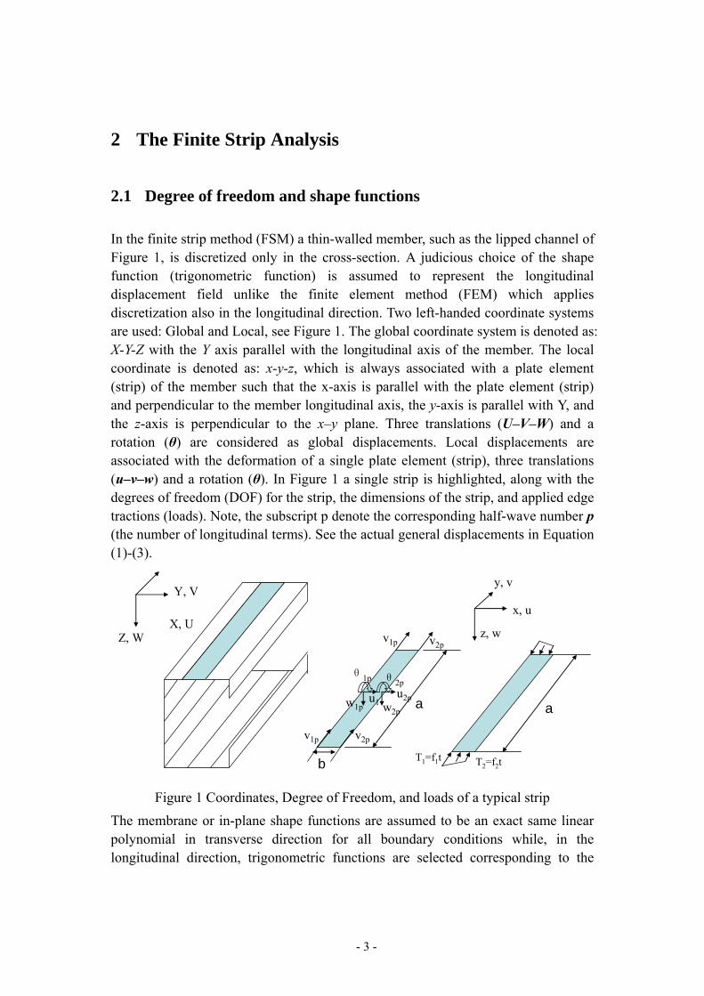
In the finite strip method (FSM) a thin-walled member, such as the lipped channel of Figure 1, is discretized only in the cross-section. A judicious choice of the shape function (trigonometric function) is assumed to represent the longitudinal displacement field unlike the finite element method (FEM) which applies discretization also in the longitudinal direction. Two left-handed coordinate systems are used: Global and Local, see Figure 1. The global coordinate system is denoted as: X-Y-Z with the Y axis parallel with the longitudinal axis of the member. The local coordinate is denoted as: x-y-z, which is always associated with a plate element (strip) of the member such that the x-axis is parallel with the plate element (strip) and perpendicular to the member longitudinal axis, the y-axis is parallel with Y, and the z-axis is perpendicular to the x–y plane. Three translations (U–V–W) and a rotation (θ) are considered as global displacements. Local displacements are associated with the deformation of a single plate element (strip), three translations (u–v–w) and a rotation (θ). In Figure 1 a single strip is highlighted, along with the degrees of freedom (DOF) for the strip, the dimensions of the strip, and applied edge tractions (loads). Note, the subscript p denote the corresponding half-wave number p (the number of longitudinal terms). See the actual general displacements in Equation (1)-(3).

w1pu1

θ1p

w2p

u2p

θ2p

v1p v2p

a

b

y, v

x, u

z, w

Y, V

X, UZ, W v1p v2p

T1=f1t T2=f2t

a

Figure 1 Coordinates, Degree of Freedom, and loads of a typical strip The membrane or in-plane shape functions are assumed to be an exact same linear polynomial in transverse direction for all boundary conditions while, in the longitudinal direction, trigonometric functions are selected corresponding to the

- 4 -

pre-set boundary conditions. For the out-of-plane displacement, the shape function is set as a cubic polynomial in transverse direction for all boundary conditions while trigonometric functions are selected corresponding to the pre-set boundary conditions of loaded edges in the longitudinal direction. The explicit definitions of the general displacements, u, v and w, are addressed in terms of the displacement at the nodes and selected shape functions as below:

pp

pm

pY

uu

bx

bxu

⎭⎬⎫

⎩⎨⎧⎥⎦⎤

⎢⎣⎡ −= ∑

= 2

1

1)1( (1)

p

pp

pm

p

aYvv

bx

bxv

μ'

2

1

1

)1(⎭⎬⎫

⎩⎨⎧⎥⎦⎤

⎢⎣⎡ −=∑

=

(2)

p

p

p

p

p

m

pY

w

w

bx

bxw

⎪⎪⎭

⎪⎪⎬

⎫

⎪⎪⎩

⎪⎪⎨

⎧

⎥⎦

⎤⎢⎣

⎡−++=∑

=

2

2

1

1

12

2

3

3

2

2

2

2

3

3

2

2

)bx-

bxx(2

b3x)

bx

b2x-x(12

b3x-1

θ

θ (3)

where μp=pπ, and p is the half-wave number, which also stands for certain half-wavelength along the longitudinal direction; m is the maximum half-wave number employed in the analysis, which is a finite positive integer; Ym is the shape function in the longitudinal direction to represent the longitudinal displacement field [2], and also

aypYpπsin= for the simply-simply supported boundary condition (S-S)

ay

aypYp

ππ sinsin= for the clamped-clamped supported boundary condition (C-C)

ayp

pp

aypYp

ππ sin1)1(sin ⎟⎟⎠

⎞⎜⎜⎝

⎛ ++

+= for the simply-clamped supported boundary

condition (S-C)

a

ypYp

π)21(

cos1−

−= for the clamped-free supported boundary condition (C-F)

ay

a

ypYp 2

sin)

21(

sin ππ−= for the clamped-guided supported boundary condition

(C-G) The expressions of u, v and w can be put in the general vector form such that

[ ] [ ]∑∑==

=

⎪⎪⎭

⎪⎪⎬

⎫

⎪⎪⎩

⎪⎪⎨

⎧

=⎭⎬⎫

⎩⎨⎧ m

p

puvuv

m

p

p

p

p

p

uv dN

vuvu

Nvu

11

2

2

1

1

and [ ] [ ]∑∑==

=

⎪⎪⎭

⎪⎪⎬

⎫

⎪⎪⎩

⎪⎪⎨

⎧

=m

p

pww

m

p

p

p

p

p

w dNw

w

Nw11

2

2

1

1

θ

θ (4)

- 5 -

2.2 Elastic stiffness matrix (k)

The strain in the strip consists of two portions: membrane and bending as shown below. The membrane strains, εM, are at the mid-line of the strip and governed by plane stress assumptions. The bending strains, εB, follow Kirchoff thin plate theory and zero at the mid-line, which is a function of w alone [1, 3].

BM εεε += (5)

{ } [ ] [ ]∑∑==

=

⎪⎪⎭

⎪⎪⎬

⎫

⎪⎪⎩

⎪⎪⎨

⎧

=

⎪⎪⎪

⎭

⎪⎪⎪

⎬

⎫

⎪⎪⎪

⎩

⎪⎪⎪

⎨

⎧

∂∂

+∂∂∂∂∂∂

=⎪⎭

⎪⎬

⎫

⎪⎩

⎪⎨

⎧

=m

p

puv

pm

p

p

p

p

p

uv

M

Mxy

y

x

M dB

vuvu

N

xv

yu

yvxu

M11

2

2

1

1

'

γεε

ε (6)

{ } [ ] [ ]∑∑==

=

⎪⎪⎭

⎪⎪⎬

⎫

⎪⎪⎩

⎪⎪⎨

⎧

=

⎪⎪⎪

⎭

⎪⎪⎪

⎬

⎫

⎪⎪⎪

⎩

⎪⎪⎪

⎨

⎧

∂∂∂∂∂

−

∂∂

−

=⎪⎭

⎪⎬

⎫

⎪⎩

⎪⎨

⎧

=m

p

pw

pm

p

p

p

p

p

w

B

Bxy

y

x

B dBzw

w

Nz

yxwz

ywz

xwz

B11

2

2

1

1

'

2

2

2

2

2

2 θ

θ

γεε

ε (7)

As shown above, the strains εM and εB can be written in terms of appropriate derivatives of shape functions, Nuv and Nw, and the nodal displacements, with respect to each half-wave number p. Moreover, the generalized “strain”-displacement relation can be used instead of the bending strain εB as [6]:

{ } [ ] [ ]∑∑==

=

⎪⎪⎭

⎪⎪⎬

⎫

⎪⎪⎩

⎪⎪⎨

⎧

=

⎪⎪⎪

⎭

⎪⎪⎪

⎬

⎫

⎪⎪⎪

⎩

⎪⎪⎪

⎨

⎧

∂∂∂∂∂

−

∂∂

−

=m

p

pw

pm

p

p

p

p

p

w

Be

eB dBw

w

N

yxw

yw

xw

B11

2

2

1

1

'

2

2

2

2

2

2 θ

θε (8)

Because the membrane behavior (u, v) is uncoupled from the bending behavior (w), the internal strain energy during buckling consists of two separate portions such that:

{ } { } { } { }dVdVU BV

TBMV

TM σεσε ∫∫ +=

21

21 (9)

For a constant thickness t, applying the membrane constitutive relation, { } { }MMM D εσ ][= , and the stresses(moments)-generalized “strain” relation [6], { } { }eBBeB D εσ ][= , the internal strain energy can be rewritten as following:

- 6 -

{ } [ ]{ } { } [ ]{ }∫ ∫∫ ∫ +=a b

eBBT

eB

a b

MMT

M dxdyDdxdyDtU0 00 0 2

121 εεεε (10)

where [ ]⎥⎥⎥

⎦

⎤

⎢⎢⎢

⎣

⎡=

GEEvEvE

D y

x

M

0000

21

21

and [ ]⎥⎥⎥

⎦

⎤

⎢⎢⎢

⎣

⎡

=

xy

y

x

B

DDDDD

D00

00

1

1

with yx

x

vvEE−

=11 ,

yx

y

vvE

E−

=12 ,

)1(12

3

yx

xx vv

tED−

= , )1(12

3

yx

yy vv

tED

−= ,

)1(12)1(12

33

1yx

yx

yx

xy

vvtEv

vvtEv

D−

=−

= , and 12

3GtDxy =

The elastic stiffness matrix can be readily derived from the statement of the internal strain energy such that:

( ) ( ) [ ] ( ) ( ) [ ] qw

a bqBB

TpB

Tpw

m

p

m

q

quv

a bqMM

TpM

Tpuv

m

p

m

qddxdyBDBdddxdyBDBtdU ⎟⎟⎠

⎞⎜⎜⎝

⎛+⎟⎟

⎠

⎞⎜⎜⎝

⎛= ∫ ∫∑∑∫ ∫∑∑

= == = 0 01 10 01 1 21

21

(11) or for short as:

qpqT

p

m

p

m

qdkdU

e∑∑= =

=1 1 2

1 (12)

where ⎥⎦

⎤⎢⎣

⎡= p

w

puv

p dd

d , ⎥⎦

⎤⎢⎣

⎡= q

w

quv

q dd

d and pqe

k is the elastic stiffness matrix corresponding

to half-wave numbers p and q which can be separated for membrane and bending,

⎥⎥⎦

⎤

⎢⎢⎣

⎡

⋅⋅

= pq

pqpq

eB

eM

e kk

k (13)

( ) [ ]∫ ∫=a b

qMM

TpM

pq dxdyBDBtkeM

0 0

and ( ) [ ]∫ ∫=a b

qBB

TpB

pq dxdyBDBkeB

0 0

(14)

Thus, the elastic stiffness can be concisely expressed in a form such that:

[ ]mm

pqe

kk×

= (15)

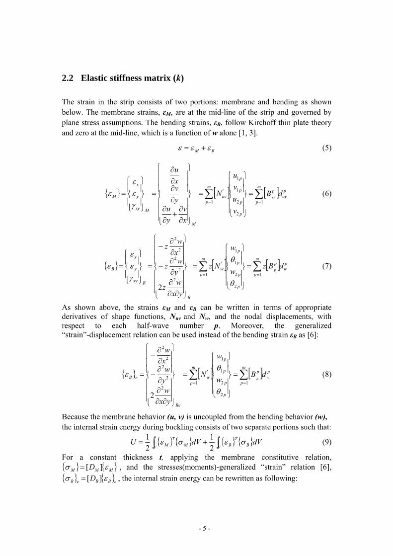
Substitution and integration yield the following closed-form expressions for the membrane, pq

eMk , and the bending, pq

eBk , elastic stiffness matrices corresponding to the

half-wave numbers p and q:

- 7 -

⎥⎥⎥⎥⎥⎥⎥⎥⎥⎥

⎦

⎤

⎢⎢⎢⎢⎢⎢⎢⎢⎢⎢

⎣

⎡

⎟⎟⎠

⎞⎜⎜⎝

⎛+⎟⎟

⎠

⎞⎜⎜⎝

⎛+⎟⎟

⎠

⎞⎜⎜⎝

⎛−⎟⎟

⎠

⎞⎜⎜⎝

⎛+−

⎟⎟⎠

⎞⎜⎜⎝

⎛+⎟

⎠⎞

⎜⎝⎛ +⎟⎟

⎠

⎞⎜⎜⎝

⎛−⎟

⎠⎞

⎜⎝⎛ +−

⎟⎟⎠

⎞⎜⎜⎝

⎛−⎟⎟

⎠

⎞⎜⎜⎝

⎛−⎟⎟

⎠

⎞⎜⎜⎝

⎛+⎟⎟

⎠

⎞⎜⎜⎝

⎛−−

⎟⎟⎠

⎞⎜⎜⎝

⎛+−⎟

⎠⎞

⎜⎝⎛ +−⎟⎟

⎠

⎞⎜⎜⎝

⎛−−⎟

⎠⎞

⎜⎝⎛ +

=

21

5

21

42

1

5

1

22

21

5

21

42

1

5

1

22

2

5

2

32511

2

5

2

32511

21

5

21

42

1

5

1

22

21

5

21

42

1

5

1

22

2

5

2

32511

2

5

2

32511

322622

223226

622322

226223

cbcGI

ccbIE

cGI

cIvE

cbcGI

ccbIE

cGI

cIvE

cGI

cIvEGbI

bIE

cGI

cIvEGbI

bIE

cbcGI

ccbIE

cGI

cIvE

cbcGI

ccbIE

cGI

cIvE

cGI

cIvEGbI

bIE

cGI

cIvEGbI

bIE

tk

xx

xx

xx

xx

pqeM

(16)

where dyYYI q

a

p∫=0

1 ; dyYYI q

a

p∫=0

''2 dyYYI

q

a

p''

03 ∫= ; dyYYI

qp

a''

0

''4 ∫= ; dyYYI

qp

a'

0

'5 ∫= (see

Appendix I for the explicit integration results).

- 8 -

⎥⎥⎥⎥⎥⎥⎥⎥⎥⎥⎥⎥⎥⎥⎥⎥⎥⎥⎥⎥

⎦

⎤

⎢⎢⎢⎢⎢⎢⎢⎢⎢⎢⎢⎢⎢⎢⎢⎢⎢⎢⎢⎢

⎣

⎡

⎟⎟⎟⎟

⎠

⎞

⎜⎜⎜⎜

⎝

⎛

+

+−

−

⎟⎟⎟⎟

⎠

⎞

⎜⎜⎜⎜

⎝

⎛

−

−+

+−

⎟⎟⎟⎟

⎠

⎞

⎜⎜⎜⎜

⎝

⎛

−

−+

+

⎟⎟⎟⎟

⎠

⎞

⎜⎜⎜⎜

⎝

⎛

+

−−

−

⎟⎟⎟⎟

⎠

⎞

⎜⎜⎜⎜

⎝

⎛

−

−+

+−

⎟⎟⎟⎟

⎠

⎞

⎜⎜⎜⎜

⎝

⎛

+

+−

−

⎟⎟⎟⎟

⎠

⎞

⎜⎜⎜⎜

⎝

⎛

−

++

+−

⎟⎟⎟⎟

⎠

⎞

⎜⎜⎜⎜

⎝

⎛

−

++

+−

⎟⎟⎟⎟

⎠

⎞

⎜⎜⎜⎜

⎝

⎛

−

−+

+

⎟⎟⎟⎟

⎠

⎞

⎜⎜⎜⎜

⎝

⎛

−

++

+−

⎟⎟⎟⎟

⎠

⎞

⎜⎜⎜⎜

⎝

⎛

+

+−

−

⎟⎟⎟⎟

⎠

⎞

⎜⎜⎜⎜

⎝

⎛

+

+−

−

⎟⎟⎟⎟

⎠

⎞

⎜⎜⎜⎜

⎝

⎛

+

−−

−

⎟⎟⎟⎟

⎠

⎞

⎜⎜⎜⎜

⎝

⎛

−

++

+−

⎟⎟⎟⎟

⎠

⎞

⎜⎜⎜⎜

⎝

⎛

+

+−

−

⎟⎟⎟⎟

⎠

⎞

⎜⎜⎜⎜

⎝

⎛

+

+−

−

=

54

46

314

214

12

53

45

213

313

1

54

46

314

214

12

53

45

313

213

1

53

45

313

213

1

52

44

312

212

1

53

45

313

213

1

52

44

312

212

1

54

46

314

214

12

53

45

313

213

1

54

46

314

214

12

53

45

213

313

1

53

45

313

213

1

52

44

312

212

1

53

45

313

213

1

52

44

312

212

1

3

224

456

561680

168

2242

4622520

56

314

14840

168

1342

422520

168

2242

4622520

2016

156504

5045040

168

1342

422520

2016

54504

5045040

56

314

14840

168

1342

422520

224

456

561680

168

2242

4622520

168

1342

422520

2016

54504

5045040

168

2242

4622520

2016

156504

5045040

4201

IDb

IDbIDb

IDbIDb

IDb

IDbIDb

IDbIbD

IDb

IDbIDb

IDbIDb

IDb

IDbIDb

IDbIbD

IDb

IDbIDb

IDbIbD

IDb

IDbIDb

IDbID

IDb

IDbIDb

IDbIbD

IDb

IDbIDb

IDbID

IDb

IDbIDb

IDbIDb

IDb

IDbIDb

IDbIbD

IDb

IDbIDb

IDbIDb

IDb

IDbIDb

IDbIbD

IDb

IDbIDb

IDbIbD

IDb

IDbIDb

IDbID

IDb

IDbIDb

IDbIbD

IDb

IDbIDb

IDbID

bk

xy

y

x

xy

y

x

xy

y

x

xy

y

x

xy

y

x

xy

y

x

xy

y

x

xy

y

x

xy

y

x

xy

y

x

xy

y

x

xy

y

x

xy

y

x

xy

y

x

xy

y

x

xy

y

x

pqeB (17)

where a

pc π=1 ;

aqc π

=2 ; dyYYI q

a

p∫=0

1 ; dyYYI q

a

p∫=0

''2 ; dyYYI

q

a

p''

03 ∫= ; dyYYI

qp

a''

0

''4 ∫= ; dyYYI

qp

a'

0

'5 ∫=

- 9 -

2.3 Geometric stiffness matrix (kg)

As shown in Figure 1, the strip is loaded with linearly varying edge tractions (T1, T2). Two methods can be employed to determine the geometric stiffness matrix for a plate strip: in terms of higher order strain or equivalently by forming the additional potential energy due to in-plane forces (the edge tractions T1, T2). The latter is the method used here. The potential energy Vp due to these edge forces T1 and T2 during the buckling is expressed as [1, 2]:

dxdyyw

yv

yu

bxTTTV

a b

P⎥⎥⎦

⎤

⎢⎢⎣

⎡⎟⎟⎠

⎞⎜⎜⎝

⎛∂∂

+⎟⎟⎠

⎞⎜⎜⎝

⎛∂∂

+⎟⎟⎠

⎞⎜⎜⎝

⎛∂∂

−−= ∫ ∫222

0 0211 ))((

21 (18)

The derivatives of the displacements can be written in terms of appropriate derivatives of shape functions, Nuv and Nw, and the nodal displacements, with respect to each half-wave number p, similar to the elastic stiffness solution. To illustrate this, for bending, the derivative of w can be expressed as,

[ ] [ ] [ ] [ ]⎪⎪⎭

⎪⎪⎬

⎫

⎪⎪⎩

⎪⎪⎨

⎧

⎪⎪⎭

⎪⎪⎬

⎫

⎪⎪⎩

⎪⎪⎨

⎧

=

⎟⎟⎟⎟⎟

⎠

⎞

⎜⎜⎜⎜⎜

⎝

⎛

⎪⎪⎭

⎪⎪⎬

⎫

⎪⎪⎩

⎪⎪⎨

⎧

=

⎟⎟⎟⎟⎟

⎠

⎞

⎜⎜⎜⎜⎜

⎝

⎛

⎪⎪⎭

⎪⎪⎬

⎫

⎪⎪⎩

⎪⎪⎨

⎧

=⎟⎟⎠

⎞⎜⎜⎝

⎛∂∂ ∑∑∑∑

= ===

q

q

q

q

qB

m

p

m

q

TpB

T

p

p

p

p

m

p

p

p

p

p

pB

m

p

p

p

p

p

w

w

GGw

w

w

w

Gw

w

Nyw

w

2

2

1

1

1 1

2

2

1

12

1

2

2

1

12

1

2

2

1

1

'2

θ

θ

θ

θ

θ

θ

θ

θ(19)

For membrane, the derivative of u and v can be given as:

[ ] [ ] [ ] [ ]⎪⎪⎭

⎪⎪⎬

⎫

⎪⎪⎩

⎪⎪⎨

⎧

⎪⎪⎭

⎪⎪⎬

⎫

⎪⎪⎩

⎪⎪⎨

⎧

=

⎟⎟⎟⎟⎟

⎠

⎞

⎜⎜⎜⎜⎜

⎝

⎛

⎪⎪⎭

⎪⎪⎬

⎫

⎪⎪⎩

⎪⎪⎨

⎧

=

⎟⎟⎟⎟⎟

⎠

⎞

⎜⎜⎜⎜⎜

⎝

⎛

⎪⎪⎭

⎪⎪⎬

⎫

⎪⎪⎩

⎪⎪⎨

⎧

=

⎪⎪

⎭

⎪⎪

⎬

⎫

⎪⎪

⎩

⎪⎪

⎨

⎧

⎟⎟⎠

⎞⎜⎜⎝

⎛∂∂

⎟⎟⎠

⎞⎜⎜⎝

⎛∂∂

∑∑∑∑= ===

q

q

q

q

qM

m

p

m

q

TpM

T

p

p

p

p

m

p

p

p

p

p

pM

m

p

p

p

p

p

vuvu

GG

vuvu

vuvu

G

vuvu

N

yvyu

uv

2

2

1

1

1 1

2

2

1

12

1

2

2

1

12

1

2

2

1

1

'2

2

(20)

The potential energy Vp then can be rewritten as

[ ] [ ] dxdydGGdbxTTTV q

qm

p

m

q

TpTp

a b

P ⎟⎟⎠

⎞⎜⎜⎝

⎛−−= ∑∑∫ ∫

= =1 10 0211 ))((

21

[ ] [ ] qqTp

a bm

p

m

q

Tp ddxdyGG

bxTTTd ⎟⎟

⎠

⎞⎜⎜⎝

⎛−−= ∫ ∫∑∑

= = 0 0211

1 1))((

21 (21)

or for short as:

qpqg

m

p

m

q

Tpp dkdV ∑∑

= =

=1 1 2

1 (22)

where [ ]⎥⎥⎦

⎤

⎢⎢⎣

⎡

⋅⋅

= p

pp

B

M

GG

G and [ ]⎥⎥⎦

⎤

⎢⎢⎣

⎡

⋅⋅

= q

qq

B

M

GG

G ; pqgk corresponding to half-wave

numbers p and q is broken into two parts: the membrane, pqgMk , and bending, pq

gBk ,

- 10 -

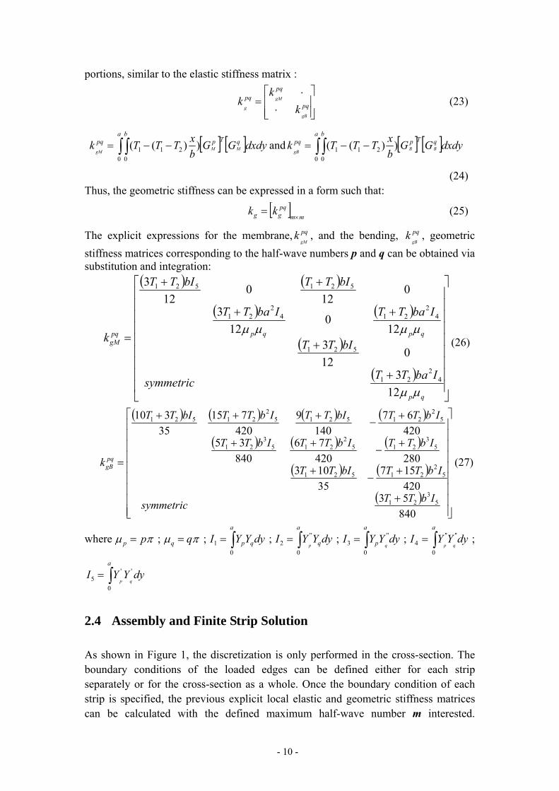
portions, similar to the elastic stiffness matrix :

⎥⎥⎦

⎤

⎢⎢⎣

⎡

⋅

⋅= pq

pqpq

gB

gM

g kk

k (23)

[ ] [ ]dxdyGGbxTTTk qTp

a bpq

MMgM ∫ ∫ −−=

0 0211 ))(( and [ ] [ ]dxdyGG

bxTTTk qTp

a bpq

BBgB ∫ ∫ −−=

0 0211 ))((

(24) Thus, the geometric stiffness can be expressed in a form such that:

[ ]mm

pqgg kk

×= (25)

The explicit expressions for the membrane, pqgM

k , and the bending, pqgB

k , geometric stiffness matrices corresponding to the half-wave numbers p and q can be obtained via substitution and integration:

( ) ( )

( ) ( )

( )

( )⎥⎥⎥⎥⎥⎥⎥⎥⎥

⎦

⎤

⎢⎢⎢⎢⎢⎢⎢⎢⎢

⎣

⎡

+

+

++

++

=

qp

qpqppqgM

IbaTTsymmetric

bITT

IbaTTIbaTT

bITTbITT

k

μμ

μμμμ

123

0123

120

123

012

012

3

42

21

521

42

2142

21

521521

(26)

( ) ( ) ( ) ( )

( ) ( ) ( )

( ) ( )

( )⎥⎥⎥⎥⎥⎥⎥⎥⎥

⎦

⎤

⎢⎢⎢⎢⎢⎢⎢⎢⎢

⎣

⎡

+

+−

+

+−

++

+−

+++

=

84053420157

35103

28042076

84035

42067

1409

420715

35310

53

21

52

21521

53

2152

2153

21

52

2152152

21521

IbTTsymmetric

IbTTbITT

IbTTIbTTIbTT

IbTTbITTIbTTbITT

k pqgB (27)

where πμ pp = ; πμ qq = ; dyYYI q

a

p∫=0

1 ; dyYYI q

a

p∫=0

''2 ; dyYYI

q

a

p''

03 ∫= ; dyYYI

qp

a''

0

''4 ∫= ;

dyYYIqp

a'

0

'5 ∫=

2.4 Assembly and Finite Strip Solution

As shown in Figure 1, the discretization is only performed in the cross-section. The boundary conditions of the loaded edges can be defined either for each strip separately or for the cross-section as a whole. Once the boundary condition of each strip is specified, the previous explicit local elastic and geometric stiffness matrices can be calculated with the defined maximum half-wave number m interested.

- 11 -

Transformations from local to global coordinates are needed to form the global elastic and geometric stiffness matrices for each strip. Thus by an appropriate summation of the global stiffness and geometric matrices with all DOFs in global coordinates, the global elastic, Ke, and geometric, Kg, stiffness matrices can be assembled and the elastic buckling problem is a typical eigenvalue problem in a form such that:

ΦΛ=Φ ge KK (28)

Where, Λ is a diagonal matrix containing the eigenvalues which are the elastic buckling loads and Φ is the matrix corresponding eigenmodes (or buckling modes) in its columns. Note, both the global elastic, Ke, and geometric, Kg, stiffness matrices are a function of the strip length a. The elastic buckling loads and mode shapes are also determined by the strip length a. In addition, different with the common CUFSM buckling curves, the results from the new developed FSM always stand for the actual lengths other than the half-wavelengths [1].

3 Comparison of Finite Strip and Finite Element Solutions

ABAQUS thin shell element eigenbuckling analysis (FEM) are employed to calibrate the accuracy of the new developed FSM. In this section, all the eigenvalues and their corresponding buckling modes are referred to as the first lowest eigenvalues and the associated buckling modes for both FEM and FSM. The elastic buckling coefficients for plate in uniform compression are verified first, which gives us a direct sense of the accuracy of FSM. Then a thin-walled member of SSMA structural stud section [7] in axial compression, major and minor axis bending is extensively studied for clamped-clamped (C-C) boundary conditions as another example. Material property of both the plate and the thin-walled member is isotropic and homogenous with an elastic modulus 29500ksi and Poisson ratio 0.3.

3.1 The Finite Element Method

The finite element method is a very efficient and powerful approach to analyze the elastic buckling loads and mode shapes. Problems with complex geometry and boundary conditions can be solved with reasonable accuracy. Eigenvalue buckling analysis is a linear perturbation procedure. The commercial finite element package ABAQUS 6.7 is used for the elastic buckling analysis. The full content of the theory behind the buckling analysis in ABAQUS is available in ABAQUS Theory Manual [8]. ABAQUS provides two iteration methods for eigenvalue extraction: the Lanczos and Subspace methods. The Lanczos method is selected for this study because it is generally faster when a large number of eigenmodes is required. The element type employed for the study is the shell element S9R5 for its consistence on the mesh

- 12 -

sensitivity. In addition, special attention is paid on boundary conditions for different loading cases.

3.2 Verification of plate

In order to verify the accuracy of the finite strip analysis result, a plate whose result would be easily understood is analyzed in this section for both FSM and FEM. Five boundary conditions of loaded edges, Simply-Simply supported (S-S), Clamped-Clamped (C-C), Simply-Clamped (S-C), Clamped-Guided (C-G), and Clamped-Free (C-F), are all included in the study. Also, the two longitudinal edges (two sides) are set to be as simply-simply supported (s-s) or clamped-clamped (c-c) boundary conditions, where lowercase letters are used to distinguish from the loaded edges. The width of the plate b is 2.5 inch and the thickness t is 0.05 inch. The analyzed length L, which is the actual length of the plate, is varying and the plate is under uniform compression at the loaded edges. The local buckling coefficient k is calculated from the equation

2

2

2

)1(12⎟⎠⎞

⎜⎝⎛

−=

bt

vEkcr

πσ (29)

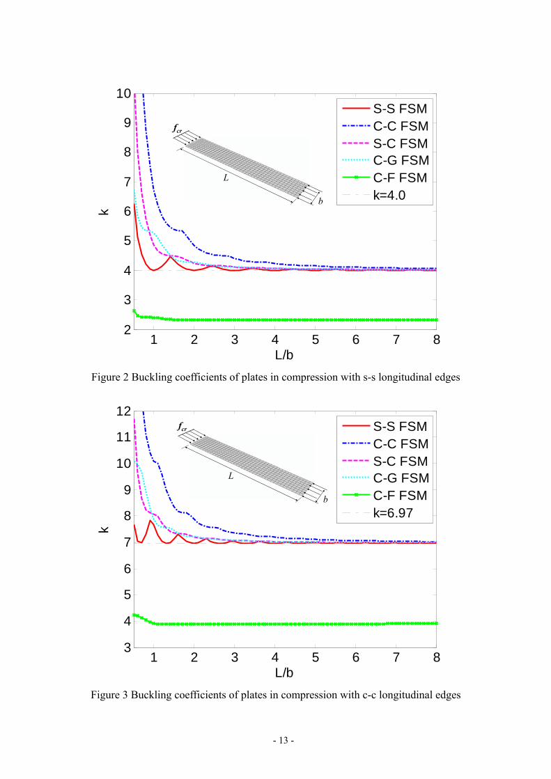
Where crσ is the critical buckling stress, t is the thickness of the plate, b is the width of the plate, E is the elastic modulus, and v is the Poisson ratio. The finite strip analyses are performed for different boundary conditions of the loaded edges and the buckling coefficients are shown in Figure 2 and Figure 3 for simply-simply (s-s) and clamped-clamped (c-c) supported boundary conditions of the longitudinal edges, respectively. As can be seen in Figure 2, when L/b equal to an integer such as 1, 2, etc., it is evident that the buckling coefficients are exactly 4 which is the same as that predicted by the plate theory for S-S loaded edges. When the aspect ratio L/b ratio is greater than 4, for all the boundary conditions of loaded edges except of C-F, the buckling coefficient is converging to 4.0, which is, in addition, in good agreement with the exact result. Moreover, when the longitudinal edges are clamped-clamped (c-c), the buckling coefficient is converging to 6.97 with the increasing of aspect ratio L/b for all boundary conditions of the loaded edges except of C-F as shown in Figure 3, which is the same as that by plate theory. For the C-F loaded edges, the buckling coefficient is converging at 2.32 for s-s longitudinal edges and at 3.90 for c-c longitudinal edges.

- 13 -

1 2 3 4 5 6 7 82

3

4

5

6

7

8

9

10

L/b

k

S-S FSMC-C FSMS-C FSMC-G FSMC-F FSMk=4.0

L

b

fcr

Figure 2 Buckling coefficients of plates in compression with s-s longitudinal edges

1 2 3 4 5 6 7 83

4

5

6

7

8

9

10

11

12

L/b

k

S-S FSMC-C FSMS-C FSMC-G FSMC-F FSMk=6.97

L

b

fcr

Figure 3 Buckling coefficients of plates in compression with c-c longitudinal edges

- 14 -

Although the finite strip analysis results are verified to be the same as the theoretical solutions, it is still worth to compare with the finite element results. In addition to the comparison of buckling coefficient, the check of the buckling shapes also has the explicit significance as an evidence of the accuracy of the finite strip method. Figure 4 shows the local buckling coefficient k by the finite strip and finite element methods for clamped-clamped loaded edges (C-C) and simply-simply supported longitudinal edges (s-s) (for other loaded edges, see Appendix II). The buckling coefficient of the finite element method is always 0.5% lower than that of the finite strip method when aspect ratio L/b is bigger than 2. The reason of this is that the shear strain is generally included in the finite element analysis while neglected in the finite strip analysis. Except of this small difference, the buckling coefficients of the finite strip and finite element results almost coincide with each other as shown in Figure 4. Figure 5 show the first buckling modes of the finite strip and finite element results, respectively, when the aspect ratio L/b is equal to 5. Clearly, the buckling shapes are almost identical and the controlling half-wave number shall be 5 as can be seen from the buckling shapes because there are five half-waves and the half-wavelength of each half-wave seems to be almost the same. (Note, the controlling half-wave numbers can be determined from the participation of each half-wave number, and will be discussed detailedly later.)

1 2 3 4 5 6 7 82

3

4

5

6

7

8

L/b

K

C-C, s-s, FSMC-C, s-s, FEMk=4.0

Figure 4 Buckling coefficients FEM and FSM results

- 15 -

(a) Mode shape of FEM result at L/b=5 (b) Mode shape of FSM result at L/b=5 Figure 5 Buckling mode shapes of FEM and FSM at L/b=5

Figure 6 shows the local buckling coefficient k by the finite strip and finite element methods for clamped-clamped loaded edges (C-C) and clamped-clamped longitudinal edges (c-c) (for other loaded edges, see Appendix 1). In this case, the buckling coefficient of the finite element method is always 0.67% lower than that of the finite strip method when aspect ratio L/b is bigger than 2. Still, this is due to the shear strain included in FEM. Other than this, there is no significant difference between the FSM and FEM results in terms of buckling coefficient. The buckling modes of the finite strip and finite element results are shown in Figure 7 (a) and (b), respectively, when the aspect ratio L/b is equal to 5. Clearly, the buckling shapes are almost identical and the controlling half-wave number shall be 7 as can be seen from the buckling shapes.

1 2 3 4 5 6 7 85

6

7

8

9

10

11

12

L/b

K

C-C, c-c, FSMC-C, c-c, FEMk=6.97

Figure 6 Buckling coefficients FEM and FSM results

- 16 -

(a) Mode shape of FEM result at L/b=5 (b) Mode shape of FSM result at L/b=5

Figure 7 Buckling mode shapes of FEM and FSM at L/b=5

3.3 Verification of thin-walled members

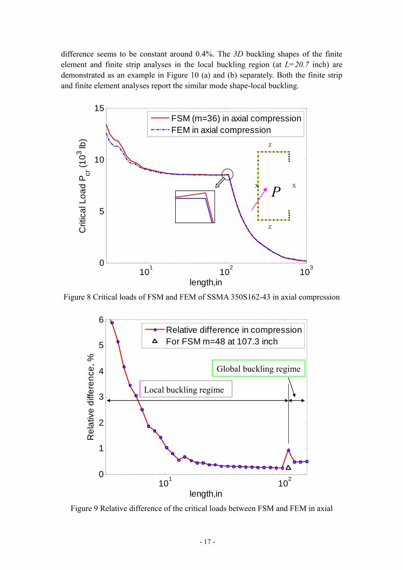
To further highlight the accuracy of the finite strip method and provide a more direct comparison between FSM and FEM, a typical thin-walled member is conducted for compression and bending analyses. The section studied here is a common channel stud section from SSMA catalog: structural stud 350S162-43 [7]. The dimension of this section is that: out-to-out web depth 3.5 inch, out-to-out flange width 1.625 inch, out-to-out lips length 0.5 inch and thickness 0.0451 inch. The section is modeled as a straight-line model, which means no round corner at the sectional lines. Three loading cases are generally considered, which are the axial compression, X-X axial bending, and Z-Z axial bending (the lips in compression). Figure 8 shows the eigenvalue buckling analysis results by both finite strip and finite element methods for the section in axial compression. The relative difference of the critical loads is plotted in Figure 9. Because there is really no practical importance when the unbraced length of the column is 12 ft longer, the relative differences are not shown in Figure 9 when the column length is 12 ft longer. Although, the buckling shapes are not shown for all the lengths here, we do investigate them and label the buckling region in Figure 9. As can be seen, there is no distinct distortional buckling region along the length. The buckling shape directly transfer from local to global buckling modes at L=107.3 inch. In the local buckling region, when the column is too short, the difference between the finite strip and finite element results are relatively big as shown in Figure 9; when the column length is larger than 15 inch, the relative difference seems to be constant around 0.3% in the rest of the local buckling region. The only exception is at L=107.3 inch where the buckling mode is still local buckling mode but the relative difference of the finite strip and finite element results is unevenly larger as shown in Figure 9 (as also can be seen from the zoom-in look at L=107.3 in Figure 8, there is a small protrusion of the finite strip results.). However, after we increase the half-wave number m to 48 in the finite strip analysis, the relative difference is reduced to 0.24%. This will be discussed more when studying the half-wave number participation later. In the global buckling region, the relative

- 17 -

difference seems to be constant around 0.4%. The 3D buckling shapes of the finite element and finite strip analyses in the local buckling region (at L=20.7 inch) are demonstrated as an example in Figure 10 (a) and (b) separately. Both the finite strip and finite element analyses report the similar mode shape-local buckling.

101 102 1030

5

10

15

length,in

Crit

ical

Loa

d P cr

(103 lb

)

FSM (m=36) in axial compressionFEM in axial compression

X X

Z

Z

P

Figure 8 Critical loads of FSM and FEM of SSMA 350S162-43 in axial compression

101 1020

1

2

3

4

5

6

length,in

Rel

ativ

e di

ffere

nce,

%

Relative difference in compressionFor FSM m=48 at 107.3 inch

Local buckling regime

Global buckling regime

Figure 9 Relative difference of the critical loads between FSM and FEM in axial

- 18 -

compression

(a) Buckling shape of FEM (b) Buckling shape of FSM Figure 10 3D Buckling mode shapes of FEM and FSM at L=20.7 inch in axial

compression For the section in X-X axis bending, the eigenvalue buckling analysis results by both finite strip and finite element methods are plotted in Figure 11. The relative difference of the critical loads is shown in Figure 12. The relative differences are only shown in Figure when the beam span is under 20 ft for there is really no practical importance when the unbraced length of the beam is 20 ft longer. The buckling regions are also labeled in Figure 12. There are three distinct buckling regions for local, distortional and global buckling modes. The clear transitions can also been seen in Figure 12 at L= 29.5 inch and L=95.4 inch. Similar to the case when the section is in axial compression, when the beam is too short, the difference between the finite strip and finite element results are relatively big in the local buckling region as shown in Figure 12; when the beam span is larger than 10 inch, the relative difference seems to be constant around 0.6% in the rest of the local buckling region. The relative differences in distortional buckling region are likely to be around 0.2% for most of them. In the global buckling region, the relative difference seems to be constant around 0.5%. In addition, the 3D buckling shapes of the finite element and finite strip analyses in the distortional buckling region (at L=42 inch) are demonstrated as an example in Figure 13 (a) and (b) separately. Again, both the finite strip and finite element analyses report the similar mode shape-distortional buckling.

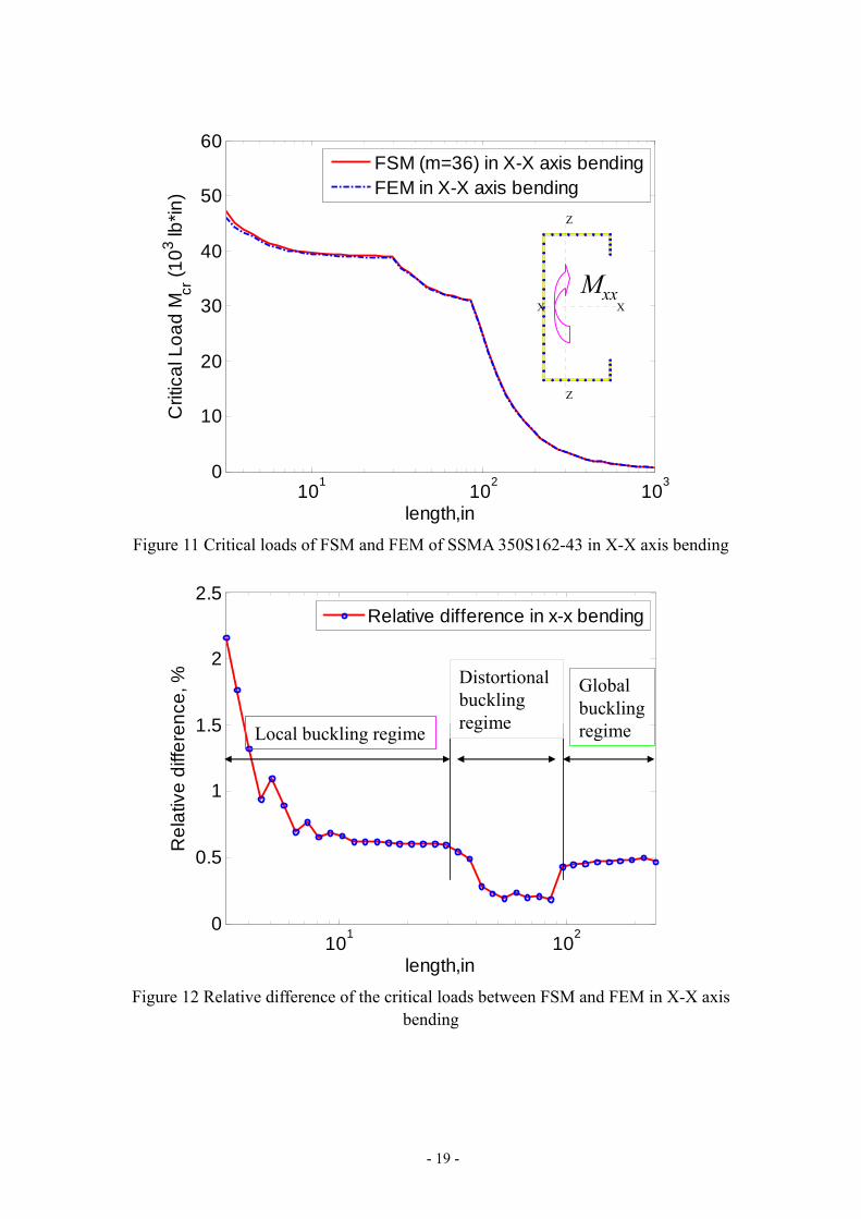
- 19 -

101 102 1030

10

20

30

40

50

60

length,in

Crit

ical

Loa

d M

cr (1

03 lb*in

)

FSM (m=36) in X-X axis bendingFEM in X-X axis bending

X X

Z

Z

Mxx

Figure 11 Critical loads of FSM and FEM of SSMA 350S162-43 in X-X axis bending

101 1020

0.5

1

1.5

2

2.5

length,in

Rel

ativ

e di

ffere

nce,

%

Relative difference in x-x bending

Local buckling regime

Distortional buckling regime

Global buckling regime

Figure 12 Relative difference of the critical loads between FSM and FEM in X-X axis

bending

- 20 -

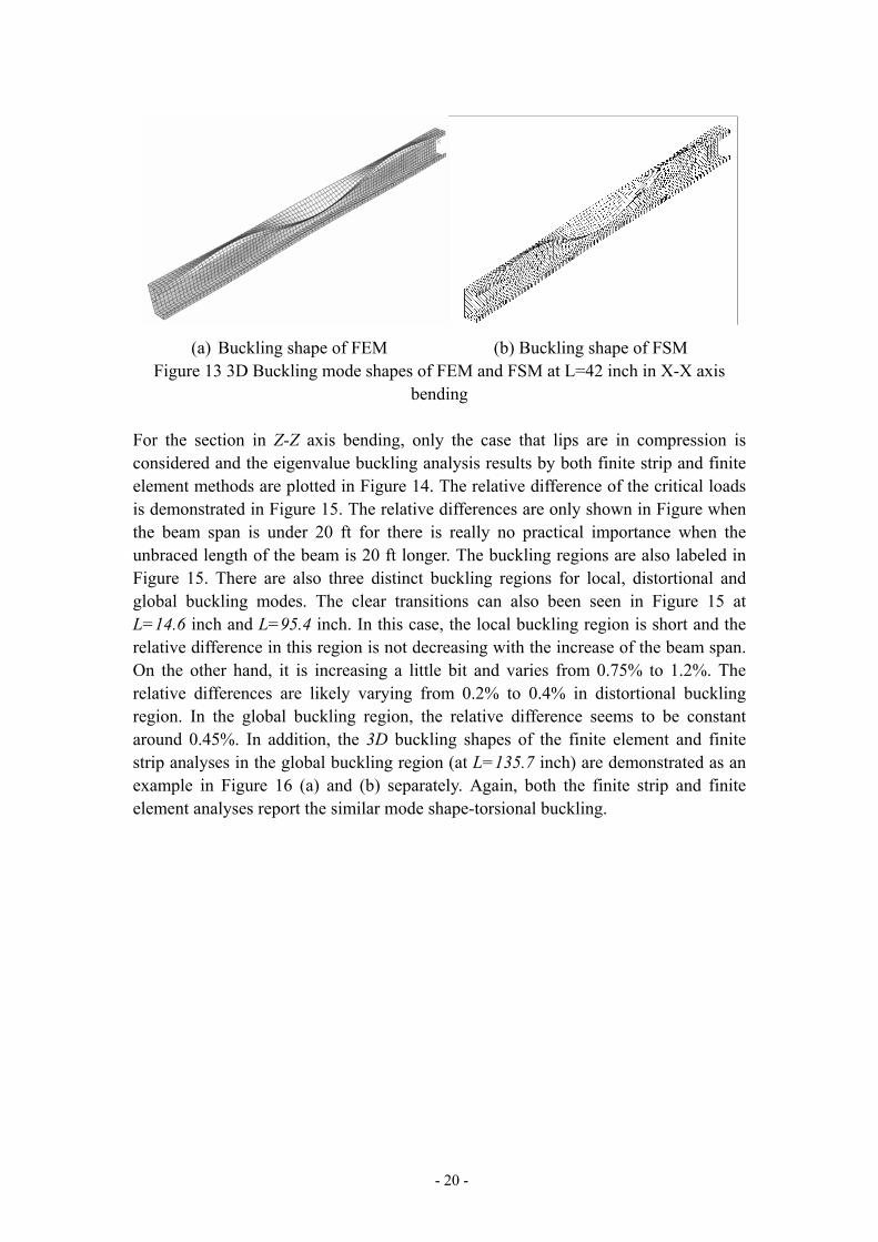
(a) Buckling shape of FEM (b) Buckling shape of FSM Figure 13 3D Buckling mode shapes of FEM and FSM at L=42 inch in X-X axis

bending For the section in Z-Z axis bending, only the case that lips are in compression is considered and the eigenvalue buckling analysis results by both finite strip and finite element methods are plotted in Figure 14. The relative difference of the critical loads is demonstrated in Figure 15. The relative differences are only shown in Figure when the beam span is under 20 ft for there is really no practical importance when the unbraced length of the beam is 20 ft longer. The buckling regions are also labeled in Figure 15. There are also three distinct buckling regions for local, distortional and global buckling modes. The clear transitions can also been seen in Figure 15 at L=14.6 inch and L=95.4 inch. In this case, the local buckling region is short and the relative difference in this region is not decreasing with the increase of the beam span. On the other hand, it is increasing a little bit and varies from 0.75% to 1.2%. The relative differences are likely varying from 0.2% to 0.4% in distortional buckling region. In the global buckling region, the relative difference seems to be constant around 0.45%. In addition, the 3D buckling shapes of the finite element and finite strip analyses in the global buckling region (at L=135.7 inch) are demonstrated as an example in Figure 16 (a) and (b) separately. Again, both the finite strip and finite element analyses report the similar mode shape-torsional buckling.

- 21 -

101 102 1030

5

10

15

20

25

30

length,in

Crit

ical

Loa

d M

cr (1

03 lb*in

)

FSM (m=36) in Z-Z axis bendingFEM in Z-Z axis bending

X X

Z

Z

Mzz

Figure 14 Critical loads of FSM and FEM of SSMA 350S162-43 in Z-Z axis bending

101 1020

0.5

1

1.5

2

length,in

Rel

ativ

e di

ffere

nce,

%

Relative difference in z-z bending

Local buckling regime

Distortional buckling regime Global

buckling regime

Figure 15 Relative difference of the critical loads between FSM and FEM in Z-Z axis

bending

- 22 -

(a) Buckling shape of FEM

(b) Buckling shape of FSM

Figure 16 3D Buckling mode shapes of FEM and FSM at L=135.7 inch in X-X axis bending

4 Half-wavelength participation in terms of half-wave

number p

As shown in Figure 5 and Figure 7, the buckling modes of the finite strip of the plate are verified with those of the finite element results. The buckling shapes are identical, at least from what can be seen so far. However, it is interestingly to notice that, in

- 23 -

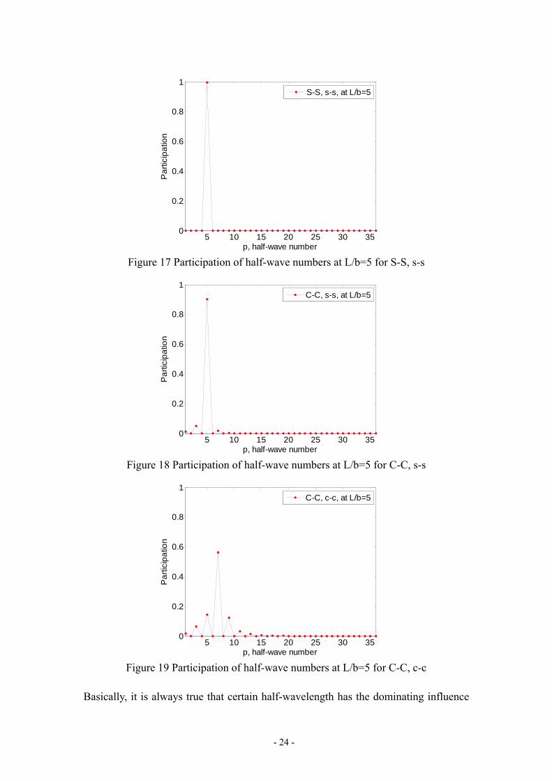
Figure 5, there are 5 half-waves and the half-wavelength of each half-wave seems almost the same. It means that 5 half-waves is the controlling mode, or in other words, when the half-wave number p equals 5, it has the most participation. While, in Figure 7, there are 7 half-waves, but the half-wavelength of each half-wave is not all the same. It seems the 5 half-waves in the middle have the same half-wavelength while the other 2 at the ends hold another half-wavelength. Although it is not easy for us to determine which half-wavelength is dominating or what the participation of this half-wavelength is, this is not a problem for the finite strip results based on the shape functions employed. The participation of each half-wavelength in terms of half-wave number p can be easily calculated from the buckling shape. Figure 18 shows the participation of half-wave number p for the clamped-clamped loaded edges (C-C) and simply-simply supported longitudinal edges (s-s) at aspect ratio L/b=5, and Figure 19 shows the participation of half-wave number p for the clamped-clamped loaded edges (C-C) and clamped-clamped longitudinal edges (c-c) at aspect ratio L/b=5. To also better illustrate how the coupling happens, the participation of half-wave number p is plotted in Figure 17 for the simply-simply supported loaded edges (S-S) and simply-simply supported longitudinal edges (s-s) at aspect ratio L/b=5. Clearly, no coupling happens when the boundary conditions are S-S loaded edges and s-s longitudinal edges as shown in Figure 17, and the controlling half-wave number is only 5, which means that the controlling half-wavelength is exactly the width b of the plate. For the boundary condition of C-C loaded edges and s-s longitudinal edges, the dominating half-wave number is still 5. However, there are several other half-wave numbers having contribution as well, especially 1, 3 and 7. They add up 10% of the total contribution of the mode shape. Thus, although directly observing of the mode shape seems the half-wavelength of each wave is the same, the analysis of the participation reveals it is not. Several other half-wavelengths (in terms of half-wave number) have significant contribution, too. This can be further illustrated by the case when the boundary conditions are C-C loaded edges and c-c longitudinal edges as shown in Figure 19. Although the dominating half-wave number is 7, more half-wave numbers involve in the mode shape and add up 42% of the total contribution, specially 5 and 9. All of this contribution makes the mode coupled by different half-wavelengths.

- 24 -

5 10 15 20 25 30 350

0.2

0.4

0.6

0.8

1

p, half-wave number

Par

ticip

atio

n

S-S, s-s, at L/b=5

Figure 17 Participation of half-wave numbers at L/b=5 for S-S, s-s

5 10 15 20 25 30 350

0.2

0.4

0.6

0.8

1

p, half-wave number

Par

ticip

atio

n

C-C, s-s, at L/b=5

Figure 18 Participation of half-wave numbers at L/b=5 for C-C, s-s

5 10 15 20 25 30 350

0.2

0.4

0.6

0.8

1

p, half-wave number

Par

ticip

atio

n

C-C, c-c, at L/b=5

Figure 19 Participation of half-wave numbers at L/b=5 for C-C, c-c

Basically, it is always true that certain half-wavelength has the dominating influence

- 25 -

on the buckling mode. In other words, for certain lengths, certain half-wave numbers p should have the most contribution of the buckling mode. First, let us examine the case of the s-s longitudinal edges. It is clear that in the S-S and s-s plate case, the only controlling half-wavelength is exactly the width b of the plate. When the plate length L is 5 times of b, the dominating half-wave number p is exactly 5 as also demonstrated in Figure 17. Even when the boundary conditions of the loaded edges change to C-C, the dominating half-wave number p is still 5, although there are some half-wave numbers around 5 have contributions as well because of the coupling between each half-wave numbers as shown in Figure 18. Now, let us set m=1 and the boundary conditions of the plate at the loaded edges as S-S and the longitudinal edges as c-c, then perform the finite strip analysis again. This is exactly the same solution as CUFSM and the length of the plate can be seen as half-wavelength. The buckling curve is shown in Figure 20. The first local minimum is the half-wavelength of local buckling, which is 1.7 inch. Similar to the s-s longitudinal edges, the dominating half-wave number p should be around the closest integer of L/1.7. In the case L=5b, which is 12.5 inch, the dominating half-wave number p should be around 7 and half-wave numbers around 7 should have large contribution. This is evidently verified by Figure 19.

100 1010

200

400

600

800

1000

1.7,74.37

Half-wavelength,in

σ cr

m=1 for S-S, c-c

Figure 20 Buckling curve of a plate under uniform compression for S-S, c-c boundary

condition Thus, to be general and applied to all kinds of sections, not just only for plate, a summary of above analyses can be rephrased as: assume that Lcrl, Lcrd, and Lcre are the half-wavelength of local, distortional and global buckling when the loaded edges are S-S and m=1 (The same as CUFSM analysis), depending on the buckling mode, the dominating half-wave numbers are near one of there values: L/ Lcrl, L/ Lcrd, and L/ Lcre, where L is the actual length of the plate or column or beam to be analyzed. For plate, it only involves local buckling (L/ Lcrl). For other sections, such as channel, Z, sigma, etc.. it will probably involve three of them (L/ Lcrl, L/ Lcrd, and L/ Lcre). To further highlight what have been explained above, let us examine the small protrusion of the finite strip result at L=107.3 inch in Figure 8. First, the buckling

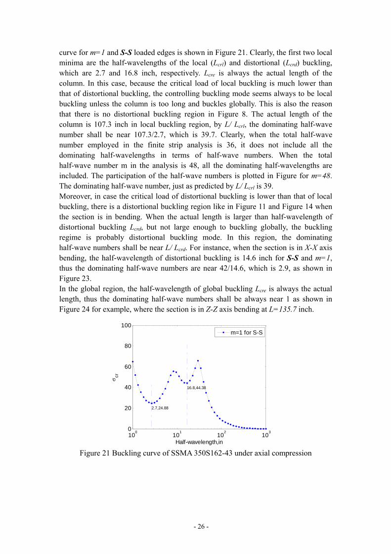
- 26 -

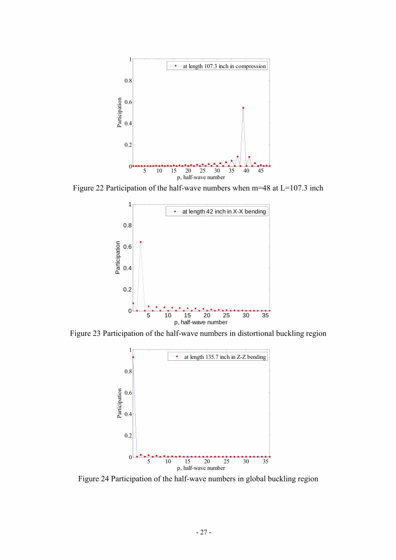
curve for m=1 and S-S loaded edges is shown in Figure 21. Clearly, the first two local minima are the half-wavelengths of the local (Lcrl) and distortional (Lcrd) buckling, which are 2.7 and 16.8 inch, respectively. Lcre is always the actual length of the column. In this case, because the critical load of local buckling is much lower than that of distortional buckling, the controlling buckling mode seems always to be local buckling unless the column is too long and buckles globally. This is also the reason that there is no distortional buckling region in Figure 8. The actual length of the column is 107.3 inch in local buckling region, by L/ Lcrl, the dominating half-wave number shall be near 107.3/2.7, which is 39.7. Clearly, when the total half-wave number employed in the finite strip analysis is 36, it does not include all the dominating half-wavelengths in terms of half-wave numbers. When the total half-wave number m in the analysis is 48, all the dominating half-wavelengths are included. The participation of the half-wave numbers is plotted in Figure for m=48. The dominating half-wave number, just as predicted by L/ Lcrl is 39. Moreover, in case the critical load of distortional buckling is lower than that of local buckling, there is a distortional buckling region like in Figure 11 and Figure 14 when the section is in bending. When the actual length is larger than half-wavelength of distortional buckling Lcrd, but not large enough to buckling globally, the buckling regime is probably distortional buckling mode. In this region, the dominating half-wave numbers shall be near L/ Lcrd. For instance, when the section is in X-X axis bending, the half-wavelength of distortional buckling is 14.6 inch for S-S and m=1, thus the dominating half-wave numbers are near 42/14.6, which is 2.9, as shown in Figure 23. In the global region, the half-wavelength of global buckling Lcre is always the actual length, thus the dominating half-wave numbers shall be always near 1 as shown in Figure 24 for example, where the section is in Z-Z axis bending at L=135.7 inch.

100 101 102 1030

20

40

60

80

100

2.7,24.88

16.8,44.38

Half-wavelength,in

σ cr

m=1 for S-S

Figure 21 Buckling curve of SSMA 350S162-43 under axial compression

- 27 -

5 10 15 20 25 30 35 40 450

0.2

0.4

0.6

0.8

1

p, half-wave number

Parti

cipa

tion

at length 107.3 inch in compression

Figure 22 Participation of the half-wave numbers when m=48 at L=107.3 inch

5 10 15 20 25 30 350

0.2

0.4

0.6

0.8

1

p, half-wave number

Par

ticip

atio

n

at length 42 inch in X-X bending

Figure 23 Participation of the half-wave numbers in distortional buckling region

5 10 15 20 25 30 350

0.2

0.4

0.6

0.8

1

p, half-wave number

Parti

cipa

tion

at length 135.7 inch in Z-Z bending

Figure 24 Participation of the half-wave numbers in global buckling region

- 28 -

5 Extension of constrained Finite Strip Method

The objective of this section is to extend the constrained Finite Strip Method (cFSM) to all the boundary conditions, such as S-S, C-C, S-C, C-G, and C-F, for any open, single-branched thin-walled members. Based on the idea of cFSM for simply supported boundary condition by Adany and Schafer [4,5,9], the existing cFSM solutions for simply-simply boundary conditions are recast into the new generalized notation. The focus of this paper is to derive the associated constraint matrices (R) which are used to decompose different buckling modes. Once the constraint matrices (R) are constructed, the constrained FSM can be performed to the two possible applications: modal decomposition and modal identification. The derivation demonstrates that full application of cFSM to general boundary conditions is readily possible.

5.1 Buckling modes classification

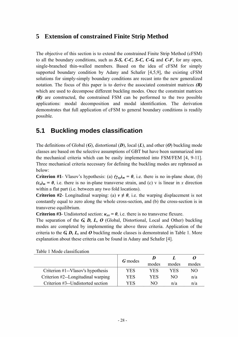
The definitions of Global (G), distortional (D), local (L), and other (O) buckling mode classes are based on the selective assumptions of GBT but have been summarized into the mechanical criteria which can be easily implemented into FSM/FEM [4, 9-11]. Three mechanical criteria necessary for defining the buckling modes are rephrased as below: Criterion #1- Vlasov’s hypothesis: (a) (γxy)m = 0, i.e. there is no in-plane shear, (b) (εx)m = 0, i.e. there is no in-plane transverse strain, and (c) v is linear in x direction within a flat part (i.e. between any two fold locations). Criterion #2- Longitudinal warping: (a) v ≠ 0, i.e. the warping displacement is not constantly equal to zero along the whole cross-section, and (b) the cross-section is in transverse equilibrium. Criterion #3- Undistorted section: κxx = 0, i.e. there is no transverse flexure. The separation of the G, D, L, O (Global, Distortional, Local and Other) buckling modes are completed by implementing the above three criteria. Application of the criteria to the G, D, L, and O buckling mode classes is demonstrated in Table 1. More explanation about these criteria can be found in Adany and Schafer [4]. Table 1 Mode classification

G modes D modes

L modes

O modes

Criterion #1--Vlasov's hypothesis YES YES YES NO Criterion #2--Longitudinal warping YES YES NO n/a Criterion #3--Undistorted section YES NO n/a n/a

- 29 -

5.2 Notations and framework of constrained FSM

The coordinate systems are still the same as the conventional FSM in Figure 1. The DOFs of global and local displacements are already explained in details in Section 2.1. For constrained FSM, Longitudinal displacements (V) will always be referred to as warping displacements and the local and global warping displacements are the same, while the other displacement components (U,W,θ) will be referred to as transverse displacements. Numbering scheme of an open, single-branched cross-section is the same as used in Anday and Schafer [4] as shown in Figure 25. It is important to distinguish between main nodes, where the two connecting strips have a nonzero angle relative to one another, and sub-nodes, where the two connecting strips are parallel. In addition, main nodes are categorized as internal main nodes or external main nodes (note, always 2 for open, single-branched thin-walled section), depending on whether two plates or only one single plate is connected to them. (Note, sub-nodes are always internal nodes.) All types of nodes are illustrated in Figure 25. Therefore, the total number of nodes (or nodal lines) is n, consisting of nm main nodes and ns sub-nodes (nm +ns = n). Also, the total number of plate elements (or strips) is (n-1) and the total number of main plate elements (or strips) is (nm-1).

1 1

2

3

i-1

i

2

i-1

i

α(i-1)

α(i)

b(i-1) , t(i-1)

b(i) , t(i)

n-2n-1

n-1

n external main nodes

internal main nodes

sub-nodes

1 1

2

nm-1nm

nm-1

nm-2

2

x

y

i+1

Figure 25 Node classification and numbering scheme

Once X and Z (global) coordinates of all the n nodes, thickness (t) of all the strips, member length (a), and material properties are known, a member can be defined. The width and angle (b and α, respectively) of the strips is calculated from the nodal coordinates. The strip orientation angle is referenced to the positive X axis. Individual nodal nodes in the following derivations are referenced by subscripts, e.g., the X coordinate of the first nodal line is: X1, while strips are referenced by superscripts in parentheses, e.g., the width of the last strip is: b(n−1), or the width of the last main strip

- 30 -

is: b(nm−1). In the general boundary case, considering that the total number of nodal lines is n, 4 displacements are assigned to each node for each half-wave number p, and the total half-wave number in the analysis is m, the total number of displacement degrees of freedom (DOF) is: TND = 4 ×m× n, instead of 4 × n such as in the case of simply supported boundary condition in Anday and Schafer [4] where it only involves one half-wave number. Similar to that in Anday and Schafer [4], relationship between the nodal displacements can be established in the form of:

MM dRd = (30)

where d is a general TND-element displacement vector, dM is a displacement vector in the reduced space, and RM is the constraint matrix related to a given mode. Of course, dM space should also be m times larger than that in case of simply supported boundary condition in Anday and Schafer [4] where it only involves one half-wave number, and the dimension of the constraint matrix should be m×m times larger. The subscript M expresses the constraint to a mode or a group of modes, i.e., M may be replaced by G, D, L, O or any combination of them, e.g. GD,GDL, etc. By introducing Equation (30) into Equation (28) in section 2, then pre-multiplying by RM

T, the constrained eigenvalue problem by the given mode or modes M can be reached,

MMgT

MMMMeT

M RKRRKR ΦΛ=Φ (31)

or in more concise form including

MMgMMMe KK ΦΛ=Φ ,, (32)

where, MeK , and MgK , are the elastic and geometric stiffness matrix of the

constrained FSM problem, respectively, and defined as MeT

MMe RKRK =, and

MgT

MMg RKRK =. ; MΛ is a diagonal matrix containing the eigenvalues for the given mode or modes, and MΦ is the matrix corresponding eigenmodes (or buckling modes) in its columns.

5.3 Derivation of the R constraint matrix

5.3.1 Derivation of RGD

5.3.1.1 Implementation of criterion #1- Vlasov’s hypothesis

When considering Criterion #1, sub-nodes are disregarded and only main nodes are considered, which are assumed to be numbered from 1 to nm. The width of the plate is referred to simply as b(i). The displacements in FSM are expressed from Equation (1) to (3) for a strip width b, which are a product of the shape function and the nodal displacements.

- 31 -

The Vlasov’s hypothesis can be written in the following forms:

0=∂∂

=xu

xε and 0=∂∂

+∂∂

=xv

yu

xyγ (33)

while the requirement of the linearity of the warping is automatically satisfied by the definition of the shape functions. Thus, the first impact of the criterion #1 can turn into

0112

1

1=

⎭⎬⎫

⎩⎨⎧⎥⎦⎤

⎢⎣⎡−=

∂∂

= ∑=

pp

pm

px Y

uu

bbxuε (34)

Since the Yp is a function of y and y is arbitrarily chosen in longitudinal direction, the coefficients of Yp must be zero, which means

ppp uuu == 21 for p=1, 2,…, m (35)

In addition, the second impact of criterion #1 can be written as

0)( '

1

21 =⎥⎥⎦

⎤

⎢⎢⎣

⎡+−+=

∂∂

+∂∂

= ∑=

p

m

p p

pppxy Ya

bv

bv

uxv

yu

μγ (36)

Since the Yp is a function of y and y is arbitrarily chosen in longitudinal direction, the coefficients of Yp must be zero, which means

p

ppppp bkvvuuu 1)( 2111 −=== for p=1, 2,…, m (37)

where apak pp // πμ == . Now, considering the i-th main nodal line, the connecting main strips are the (i-1)-th and (i)-th. Apply the notation explained before and the Equation (37), we can get

⎥⎥⎦

⎤

⎢⎢⎣

⎡⎥⎦⎤

⎢⎣⎡ −

= −

−

−−−

)1(2

)1(1

)1()1()1( 111

ip

ip

iip

ip v

vbbk

u and ⎥⎥⎦

⎤

⎢⎢⎣

⎡⎥⎦⎤

⎢⎣⎡ −

= )(2

)(1

)()()( 111

ip

ip

iip

ip v

vbbk

u (38)

Employing the connectivity and the equivalence between the local v and global V D.O.F:

⎥⎥⎥

⎦

⎤

⎢⎢⎢

⎣

⎡

⎥⎥⎥

⎦

⎤

⎢⎢⎢

⎣

⎡

−

−

=⎥⎥⎦

⎤

⎢⎢⎣

⎡

+

−

−

−−−

pi

ip

pi

ii

ii

pi

p

ip

VV

V

bb

bbku

u

)1(

)1(

)1()(

)1()1(

)(

)1(

110

0111 for p=1, 2,…, m (39)

The above equation provides relationship between the global longitudinal and local transverse displacements. Using the left-hand coordinate system, of figure, the relationship between local displacements (u, w), and the global displacements (U, W) can be expressed as

⎥⎦

⎤⎢⎣

⎡⎥⎦

⎤⎢⎣

⎡−

=⎥⎦

⎤⎢⎣

⎡WU

aaaa

wu

cossinsincos

(40)

The relationship between the global nodal displacements (U,W) and the local displacements u of the (i-1)-th and (i)-th plate elements can be expressed as following

- 32 -

based on the transformation formula above:

⎥⎦

⎤⎢⎣

⎡⎥⎦

⎤⎢⎣

⎡=

⎥⎥⎦

⎤

⎢⎢⎣

⎡ −−−

ip

ipii

ii

ip

ip

WU

aaaa

uu

)()(

)1()1(

)(

)1(

sincossincos

for p=1, 2,…, m (41)

By the equality of the left sides of Equation (40) and Equation (41) , the relationship between the longitudinal V displacements and the transverse U and W displacements are obtained as follows:

⎥⎥⎥

⎦

⎤

⎢⎢⎢

⎣

⎡

⎥⎥⎥

⎦

⎤

⎢⎢⎢

⎣

⎡

−

−

=⎥⎦

⎤⎢⎣

⎡⎥⎦

⎤⎢⎣

⎡

+

−

−

−−−−

pi

ip

pi

ii

ii

pip

ipii

ii

VV

V

bb

bbkW

Uaa

aa

)1(

)1(

)1()(

)1()1(

)()(

)1()1(

110

0111

sincossincos

(42)

The determinant of the matrix with the sin and cos terms is assumed to be Di as follow:

)sin(cossincossin )1()()()1()1()( −−− −=−= iiiiiii aaaaaaD (43)

Since the two main connecting strips always have a nonzero angle relative to one another, the case of Di =0 is excluded. We can then rewrite Equation (42) into the following form

⎥⎥⎥

⎦

⎤

⎢⎢⎢

⎣

⎡

⎥⎥⎥

⎦

⎤

⎢⎢⎢

⎣

⎡

−

−

⎥⎦

⎤⎢⎣

⎡

−−

=⎥⎦

⎤⎢⎣

⎡

+

−

−

−−

−

−

pi

ip

pi

ii

ii

ii

ii

ipip

ip

VV

V

bb

bbaaaa

DkWU

)1(

)1(

)1()(

)1()1(

)1()(

)1()(

110

011

coscossinsin1 for p=1, 2,…, m

(44) Finally, based on Equation (44), the relationship between the transverse displacements (U,W) of all the internal main nodes and the warping displacements can be generated as below:

( )

( )

( )

( )

( )

( )

( )

( )

( )

( )

( )

( )

( )

( )

( )

( )

⎥⎥⎥⎥⎥⎥⎥⎥⎥

⎦

⎤

⎢⎢⎢⎢⎢⎢⎢⎢⎢

⎣

⎡

×

⎥⎥⎥⎥⎥⎥⎥⎥⎥

⎦

⎤

⎢⎢⎢⎢⎢⎢⎢⎢⎢

⎣

⎡

××××××

⎟⎟⎠

⎞⎜⎜⎝

⎛⎟⎟⎠

⎞⎜⎜⎝

⎛−−⎟⎟

⎠

⎞⎜⎜⎝

⎛

⎟⎟⎠

⎞⎜⎜⎝

⎛⎟⎟⎠

⎞⎜⎜⎝

⎛−−⎟⎟

⎠

⎞⎜⎜⎝

⎛

=

⎥⎥⎥⎥⎥⎥

⎦

⎤

⎢⎢⎢⎢⎢⎢

⎣

⎡

−

−

−

−

pnm

pnm

pnm

p

p

p

p

pnm

pnm

p

VVV

VVV

bDbDbDbD

bDbDbDbD

k

UU

U

)(

)1(

)2(

3

2

1

32

2

32

2

22

3

22

3

22

1

22

1

12

2

12

2

)1(

)2(

3

2p

0000000000

0000sinsinsinsin0

00000sinsinsinsin

1

U

M

MMMMM

Mαααα

αααα

(45)

- 33 -

( )

( )

( )

( )

( )

( )

( )

( )

( )

( )

( )

( )

( )

( )

( )

( )

⎥⎥⎥⎥⎥⎥⎥⎥⎥

⎦

⎤

⎢⎢⎢⎢⎢⎢⎢⎢⎢

⎣

⎡

×

⎥⎥⎥⎥⎥⎥⎥⎥⎥

⎦

⎤

⎢⎢⎢⎢⎢⎢⎢⎢⎢

⎣

⎡

××××××

⎟⎟⎠

⎞⎜⎜⎝

⎛⎟⎟⎠

⎞⎜⎜⎝

⎛−−⎟⎟

⎠

⎞⎜⎜⎝

⎛

⎟⎟⎠

⎞⎜⎜⎝

⎛⎟⎟⎠

⎞⎜⎜⎝

⎛−−⎟⎟

⎠

⎞⎜⎜⎝

⎛

−=

⎥⎥⎥⎥⎥⎥

⎦

⎤

⎢⎢⎢⎢⎢⎢

⎣

⎡

−

−

−

−

pnm

pnm

pnm

p

p

p

p

pnm

pnm

p

p

VVV

VVV

bDbDbDbD

bDbDbDbD

k

WW

WW

)(

)1(

)2(

3

2

1

32

2

32

2

22

3

22

3

12

1

22

1

12

2

12

2

)1(

)2(

3

2

0000000000

0000coscoscoscos0

00000coscoscoscos

1M

MMMMM

Mαααα

αααα

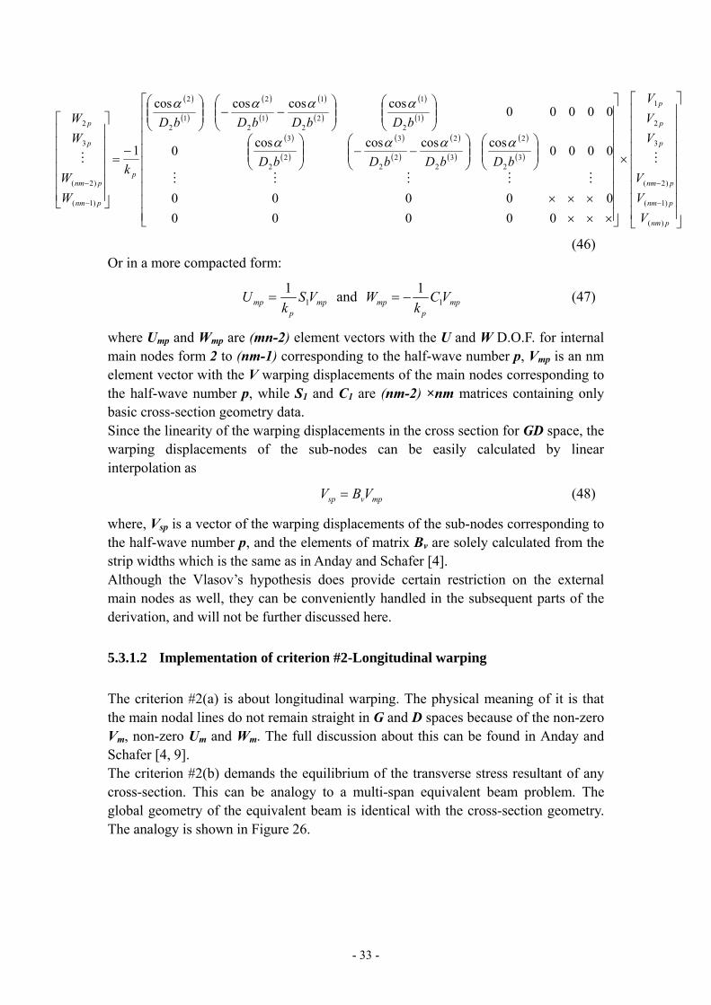
(46) Or in a more compacted form:

mpp

mp VSk

U 11

= and mpp

mp VCk

W 11

−= (47)

where Ump and Wmp are (mn-2) element vectors with the U and W D.O.F. for internal main nodes form 2 to (nm-1) corresponding to the half-wave number p, Vmp is an nm element vector with the V warping displacements of the main nodes corresponding to the half-wave number p, while S1 and C1 are (nm-2) ×nm matrices containing only basic cross-section geometry data. Since the linearity of the warping displacements in the cross section for GD space, the warping displacements of the sub-nodes can be easily calculated by linear interpolation as

mpvsp VBV = (48)

where, Vsp is a vector of the warping displacements of the sub-nodes corresponding to the half-wave number p, and the elements of matrix Bv are solely calculated from the strip widths which is the same as in Anday and Schafer [4]. Although the Vlasov’s hypothesis does provide certain restriction on the external main nodes as well, they can be conveniently handled in the subsequent parts of the derivation, and will not be further discussed here.

5.3.1.2 Implementation of criterion #2-Longitudinal warping

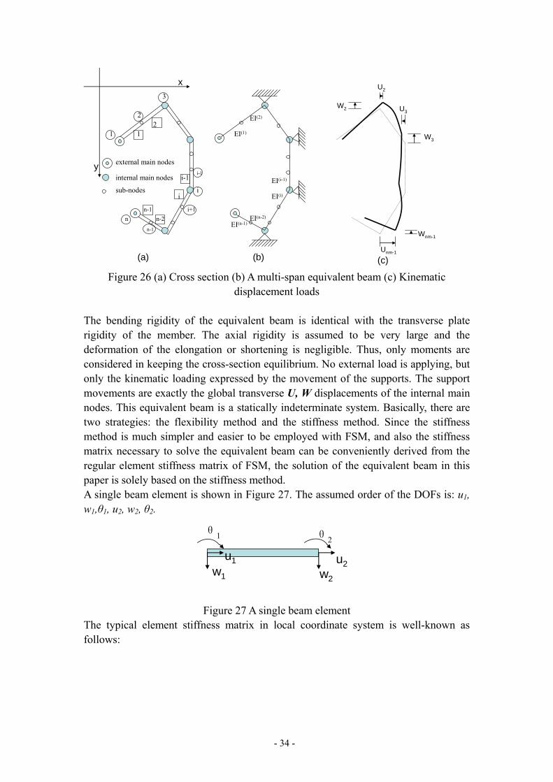
The criterion #2(a) is about longitudinal warping. The physical meaning of it is that the main nodal lines do not remain straight in G and D spaces because of the non-zero Vm, non-zero Um and Wm. The full discussion about this can be found in Anday and Schafer [4, 9]. The criterion #2(b) demands the equilibrium of the transverse stress resultant of any cross-section. This can be analogy to a multi-span equivalent beam problem. The global geometry of the equivalent beam is identical with the cross-section geometry. The analogy is shown in Figure 26.

- 34 -

1 1

2

3

i-1

i

2

i-1

i

n-2n-1

n-1

n

x

y

i+1

external main nodes

internal main nodes

sub-nodes

EI(1)

EI(2)

EI(i-1)

EI(i)

EI(n-2)

EI(n-1)

W2

U2

W3

U3

Wnm-1

Unm-1(a) (b) (c)

Figure 26 (a) Cross section (b) A multi-span equivalent beam (c) Kinematic displacement loads

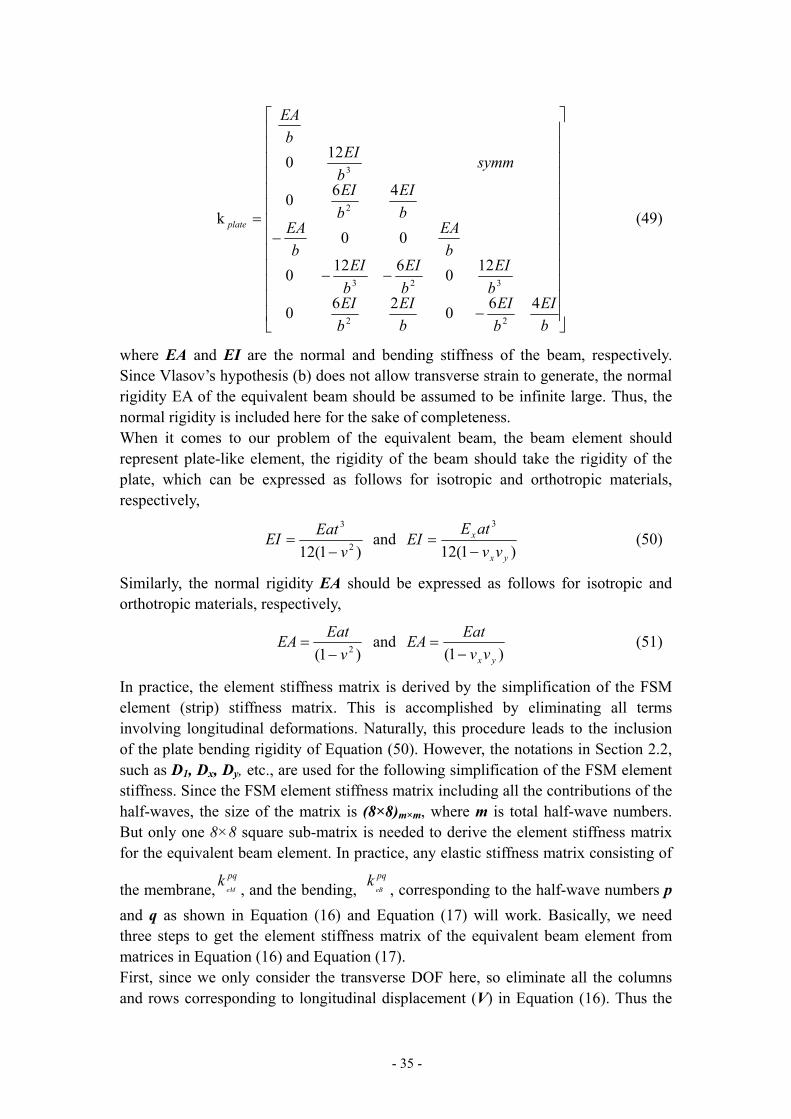
The bending rigidity of the equivalent beam is identical with the transverse plate rigidity of the member. The axial rigidity is assumed to be very large and the deformation of the elongation or shortening is negligible. Thus, only moments are considered in keeping the cross-section equilibrium. No external load is applying, but only the kinematic loading expressed by the movement of the supports. The support movements are exactly the global transverse U, W displacements of the internal main nodes. This equivalent beam is a statically indeterminate system. Basically, there are two strategies: the flexibility method and the stiffness method. Since the stiffness method is much simpler and easier to be employed with FSM, and also the stiffness matrix necessary to solve the equivalent beam can be conveniently derived from the regular element stiffness matrix of FSM, the solution of the equivalent beam in this paper is solely based on the stiffness method. A single beam element is shown in Figure 27. The assumed order of the DOFs is: u1, w1,θ1, u2, w2, θ2.

w1

u1

θ1

w2

u2

θ2

Figure 27 A single beam element

The typical element stiffness matrix in local coordinate system is well-known as follows:

- 35 -

⎥⎥⎥⎥⎥⎥⎥⎥⎥⎥⎥⎥⎥

⎦

⎤

⎢⎢⎢⎢⎢⎢⎢⎢⎢⎢⎢⎢⎢

⎣

⎡

−

−−

−=

bEI

bEI

bEI

bEI

bEI

bEI

bEI

bEA

bEA

bEI

bEI

symmbEI

bEA

plate

460260

1206120

00

460

120

k

22

323

2

3

(49)

where EA and EI are the normal and bending stiffness of the beam, respectively. Since Vlasov’s hypothesis (b) does not allow transverse strain to generate, the normal rigidity EA of the equivalent beam should be assumed to be infinite large. Thus, the normal rigidity is included here for the sake of completeness. When it comes to our problem of the equivalent beam, the beam element should represent plate-like element, the rigidity of the beam should take the rigidity of the plate, which can be expressed as follows for isotropic and orthotropic materials, respectively,

)1(12 2

3

vEatEI−

= and )1(12

3

yx

x

vvatE

EI−

= (50)

Similarly, the normal rigidity EA should be expressed as follows for isotropic and orthotropic materials, respectively,

)1( 2v

EatEA−

= and )1( yxvv

EatEA−

= (51)

In practice, the element stiffness matrix is derived by the simplification of the FSM element (strip) stiffness matrix. This is accomplished by eliminating all terms involving longitudinal deformations. Naturally, this procedure leads to the inclusion of the plate bending rigidity of Equation (50). However, the notations in Section 2.2, such as D1, Dx, Dy, etc., are used for the following simplification of the FSM element stiffness. Since the FSM element stiffness matrix including all the contributions of the half-waves, the size of the matrix is (8×8)m×m, where m is total half-wave numbers. But only one 8×8 square sub-matrix is needed to derive the element stiffness matrix for the equivalent beam element. In practice, any elastic stiffness matrix consisting of

the membrane,pqeM

k , and the bending, pqeB

k , corresponding to the half-wave numbers p and q as shown in Equation (16) and Equation (17) will work. Basically, we need three steps to get the element stiffness matrix of the equivalent beam element from matrices in Equation (16) and Equation (17). First, since we only consider the transverse DOF here, so eliminate all the columns and rows corresponding to longitudinal displacement (V) in Equation (16). Thus the

- 36 -

matrix in Equation (16) reduces into a 2×2 matrix which corresponding to degree of freedom u1p and u2p. Second, according to the applied Vlasov’s hypothesis, there should be no shear and membrane transverse strains. Thus, all the terms that contain the shear modulus G, such as the items with G and Dxy, should be eliminated in the matrix in Equation (17) and the reduced matrix by the previous step. Third, for the same reason as employed in step 1, any items related to longitudinal displacement, such as the items with Dy and D1, should be eliminated in the previous reduced matrices. (Note: in-plane terms with longitudinal modulus E2 are already eliminated by the first step.) Through the previous steps, we basically reach the stiffness matrix in the form as below

1

22

323

11

2

3

1

,

460

260

120

6120

00

460

120

k I

bD

bD

bD

bD

bD

bD

bD

btE

btE

bD

bD

symmbD

btE

xxxx

xxx

xx

x

te ×

⎥⎥⎥⎥⎥⎥⎥⎥⎥⎥⎥⎥⎥

⎦

⎤

⎢⎢⎢⎢⎢⎢⎢⎢⎢⎢⎢⎢⎢

⎣

⎡

−

−−

−= (52)

where dyYYI q

a

p∫=0

1 , which has a linear relation with a (see Appendix) and Dx is in

Equation (10). The only difference is that that the elements of the typical element stiffness matrix in Equation (52) are exactly a constant multiple, which depends on the I1, of the corresponding elements of the finite strip matrix. Since what is really important is not the real stiffness values but rather the stiffness distribution, it will not affect the results at all. The local element stiffness matrix can be transformed into the global element stiffness matrix via coordinate transformation. Finally, the global stiffness matrix Ke,t can be assembled as an appropriate summation of the global elements stiffness matrices [4, 9]. After having the global stiffness matrix assembled, the static equilibrium of the equivalent beam can be written as

ttte qdK =, (53)

where Ke,t is the global stiffness matrix, dt is the displacement vector for the transverse DOFs (U, W, θ) of the equivalent beam, and qt is the vector of the nodal forces for the same DOFs. Note, different from the case of simply supported boundary condition in Anday and Schafer where it only involves one half-wave number, the vector dt has the same dimension but different form. According to the criterion #2, the transverse stress resultants should be in equilibrium of any cross section, imagine that

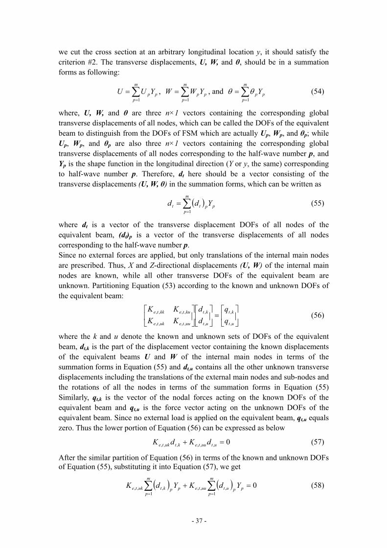
- 37 -

we cut the cross section at an arbitrary longitudinal location y, it should satisfy the criterion #2. The transverse displacements, U, W, and θ, should be in a summation forms as following:

p

m

ppYUU ∑

=

=1

, p

m

ppYWW ∑

=

=1

, and p

m

ppY∑

=

=1θθ (54)

where, U, W, and θ are three n×1 vectors containing the corresponding global transverse displacements of all nodes, which can be called the DOFs of the equivalent beam to distinguish from the DOFs of FSM which are actually Up, Wp, and θp; while Up, Wp, and θp are also three n×1 vectors containing the corresponding global transverse displacements of all nodes corresponding to the half-wave number p, and Yp is the shape function in the longitudinal direction (Y or y, the same) corresponding to half-wave number p. Therefore, dt here should be a vector consisting of the transverse displacements (U, W, θ) in the summation forms, which can be written as

( ) p

m

pptt Ydd ∑

=

=1

(55)

where dt is a vector of the transverse displacement DOFs of all nodes of the equivalent beam, (dt)p is a vector of the transverse displacements of all nodes corresponding to the half-wave number p. Since no external forces are applied, but only translations of the internal main nodes are prescribed. Thus, X and Z-directional displacements (U, W) of the internal main nodes are known, while all other transverse DOFs of the equivalent beam are unknown. Partitioning Equation (53) according to the known and unknown DOFs of the equivalent beam:

⎥⎦

⎤⎢⎣

⎡=⎥

⎦

⎤⎢⎣

⎡⎥⎦

⎤⎢⎣

⎡

ut

kt

ut

kt

uuteukte

kutekkte

qq

dd

KKKK

,

,

,

,

,,,,

,,,, (56)

where the k and u denote the known and unknown sets of DOFs of the equivalent beam, dt,k is the part of the displacement vector containing the known displacements of the equivalent beams U and W of the internal main nodes in terms of the summation forms in Equation (55) and dt,u contains all the other unknown transverse displacements including the translations of the external main nodes and sub-nodes and the rotations of all the nodes in terms of the summation forms in Equation (55) Similarly, qt,k is the vector of the nodal forces acting on the known DOFs of the equivalent beam and qt,u is the force vector acting on the unknown DOFs of the equivalent beam. Since no external load is applied on the equivalent beam, qt,u equals zero. Thus the lower portion of Equation (56) can be expressed as below

0,,,,,, =+ utuutektukte dKdK (57)

After the similar partition of Equation (56) in terms of the known and unknown DOFs of Equation (55), substituting it into Equation (57), we get

( ) ( ) 01

,,,1

,,, =+ ∑∑==

m

ppputuute

m

pppktukte YdKYdK (58)

- 38 -

Therefore, Equation (58) can be rewritten as

( ) ( )( ) 01

,,,,,, =+∑=

p

m

pputuutepktukte YdKdK (59)

Since the transverse stress resultants should be in equilibrium of any cross section at any longitudinal location y, the coefficient of Yp must be zero, which leads to

( ) ( )pktukteuuteput dKKd ,,,

1,,,

−−= for p=1,…,m (60)

Or, in more explicit form:

⎥⎦

⎤⎢⎣

⎡−=

⎥⎥⎥

⎦

⎤

⎢⎢⎢

⎣

⎡−

mp

mpukteuute

p

sp

sp

WU

KKWU

,,1

,,

θ for p=1,…,m (61)

where Usp and Wsp are two vectors of transverse displacement DOFs of the external main nodes and sub-nodes corresponding to the half-wave number p, Ump and Wmp are already known via Equation (47).

5.3.1.3 Assembly of RGD

The strategy of assembling RGD is underlined as following: 1) first assemble [RGD]p for each half-wave number p; 2) then assemble each [RGD]p into the big RGD. Each [RGD]p can be carried out its submatrices as given below

[ ] [ ]TpGD

TWspGD

TUspGD

TWmpGD

TUmpGD

TVspGD

TVmpGDpGD RRRRRRRR θ,,,,,,,= (62)

based on the preceding derivations as summarized below: 1): determination of RGD,Vmp. The simplest natural solution is set RGD,Vmp equal to the nm-order identity matrix.

IR VmpGD =, (63)

Basically, The longitudinal displacements of the main nodes, RGD,Vmp, can be arbitrarily selected. Each different leads to a specific [RGD]p, hence to a specific case vector system, however any RGD,Vmp leads to the same [RGD]p. 2): determination of RGD,Vsp from Equation (48)

VmpGDvVspGD RBR ,, = (64)

3): determination of RGD,Ump and RGD,Wmp from Equation (47)

VmpGDp

UmpGD RSk

R ,1,1

= and VmpGDp

WmpGD RCk

R ,1,1

= (65)

#4: determination of RGD,Usp, RGD,Wsp, and RGD,θp from Equation (61)

⎥⎦

⎤⎢⎣

⎡=

⎥⎥⎥

⎦

⎤

⎢⎢⎢

⎣

⎡−

WmGD

UmGDukteuute

pGD

WspGD

UspGD

RR

KKRRR

,

,,,

1,,

,

,

,

θ

(66)

- 39 -

Eventually, [RGD]p is obtained from its partitions. Then the RGD can be assembled for each half-wave number as partitioned diagonal matrix

[ ]

[ ]

[ ] ⎥⎥⎥⎥⎥⎥

⎦

⎤

⎢⎢⎢⎢⎢⎢

⎣

⎡

=

mGD

pGD

GD

GD

R

R

R

RO

O1

(67)

5.3.2 Separation of RGD into RG and RD

The constraint matrix of RGD has been derived, and consequently the definition of GD space as well. Now, we need to introduce a further transformation inside the GD space. Similar to the constrained FSM for just one half-wave number, this can be done mathematically by seeking a HGD transformation matrix which is able to represent any dGD deformation in terms of a basis, then the system of base vectors for G and D spaces can be separated as

[ ]DGGD HHH = (68)

[ ] ⎥⎦

⎤⎢⎣

⎡=

D

GDGGD d

dHHd (69)

The column vectors of HG and HD are warping distributions for global and distortional buckling modes. The HG and HD can be defined by the same strategy as we assembly the RGD: first, define the [HG]p and [HD]p corresponding the half-wave number p, which is the same as in Anday and Schafer (2008); then, assemble each [HG]p and [HD]p into the big HG and HD for all the half-wave numbers. The same as the RGD, HG and HD should be two partitioned diagonal matrices. Therefore, including Equation (30) and Equation (69) any G or D displacement vectors in the original FSM DOFs (d) can be expressed as follows:

[ ] [ ] ⎥⎦

⎤⎢⎣

⎡=⎥

⎦

⎤⎢⎣

⎡=

D

GDG

D

GDGGD d

dRR

dd

HHRd (70)

Where RGD is a partitioned diagonal matrix with the dimension (n×nm)m×m, HG is (nm×4)m×m, and HD is (nm×(nm-4))m×m. As m is the total half-wave numbers in the analysis. Consequently, the RG is a partitioned diagonal matrix with dimension (n×4)m×m and RD is (n×(nm-4))mxm, which can be expressed as below

GGDG HRR = and DGDD HRR = (71)

For each half-wave number, the [HG]p and [HD]p can be defined by the definitions of the G and D modes in terms of the warping distributions following the same strategy in Anday and Schafer [4, 5, 9], and will not be presented here. In addition, for the nm≤4, the discussion provided in Anday and Schafer [4] is still applicable here.

- 40 -

5.3.3 Derivation of RL

Derivation of RL is based on the two criteria that are applicable. First, Vlasov’s hypothesis is applied. The strict relationship between the longitudinal warping of the main nodes and the translation displacements (U, W) of the internal main nodes are achieved as shown in Equation (47). Second, the criterion #2 related to the longitudinal warping should not be satisfied, which means that (i) all the warping displacements are zero, (ii) transverse equilibrium may be violated. Based on the first condition of criterion #2 and Equation (47), the translation displacements (U, W) of all the internal nodes should be zero and also local u should be zero as well. As a consequence, translation displacements of all nodes except of internal main nodes should be restricted to the local w direction, i.e., perpendicular to the given plate element. Following the same strategy for the RGD, first, define the [RL]p corresponding the half-wave number p, which is exactly the same as in Anday and Schafer [4] because the half-wave number does not matter, and also the partitions of the is the same as [RGD]p except that here is the local buckling mode space (L) instead of GD space; then, assemble each [RL]p into the big RL for all the half-wave numbers as a portioned diagonal matrix. The non-zero partitions of [RL]p can be expressed as follows:

[ ]03, SR UspL = (72)

[ ]03, CR WspL = (73)

[ ]IR pL 0, =θ (74)

where 0 stands the partitions with zeros (of various sizes), I stands the n×n identity matrix, while S3 and C3 are the diagonal matrices (both with (ns+2) ×(ns+2) dimension). Also, S3 is expressed as diag(-sinα1,-sinα2,…) and C3 as diag(cosα1,cosα2,…), where αi is the strip angle at the location of the given i-th node.

5.3.4 Derivation of RO

The applicable criterion for O modes is the Vlasov’s hypothesis that is the transverse strains and/or the in-plane shear are not zero, and a non-linear warping distribution between two main nodes might exist. Thus, deformations of O space exhibit either transverse extension/shortening, or in-plane shear. Basically, two approaches can achieve the goal to get the constraint matrix RO. The first one is to directly apply the above considerations by a system of independent vectors with unit transverse extensions and unit shear deformations. The disadvantage of this approach is that the generated O space may overlap with other subspaces (G,D,L). In practice, a more mathematical one is used which has no overlap with other subspaces and can include transverse extensions/shortening, and in-plane shear as well. Concisely, we are looking a null space of GDL space. Although lots of orthogonal possibilities exist for

- 41 -

finding this null space, a simple and meaningful one is used to define orthogonality with respect to the stiffness matrix Ke as follow:

0=GDLeT

O RKR (75)

Since Ke and RGDL are known, the constraint matrix RO is defined although it is not unique. This is the same approach used in Anday and Schafer [4] except that in this case, combination of difference half-wave number p is included.

6 Conclusion

This paper presents the full theoretical derivation for a finite strip method (FSM) stability solution which can be applied to various boundary conditions: simply-simply, clamped-clamped, simply-clamped, clamped-guided, and clamped-free. The derivation is depended upon the selection of the longitudinal shape functions to represent the boundary conditions. In the provided solution, the shape functions are built upon those of Bradford and Azhari. The notation of Cheung and Tham can also be possible employed to connect to the broader literature of FSM. In the notation of Cheung and Tham the elastic and geometric stiffness matrices are provided in a general form with only specific integrals remaining boundary condition specific and the total half-wave numbers you want to include in the solution. The new boundary conditions are implemented in a custom version of CUFSM and verification problems are provided against eigenbuckling shell finite element analysis solutions implemented in ABAQUS. First, the elastic buckling coefficients for plate in uniform compression are verified first for all the boundary conditions when the longitudinal boundary conditions are set to be simply-simply supported or clamped-clamped. The results are in well agreement with those of the plate theory. The results are also calibrated with the FEM solutions. The well agreement is also found both for the buckling coefficients and the buckling mode shapes. The only small difference is the buckling coefficients that FEM solution is always a little lower (within 1%) than that of the FSM solution because the shear strain effect is included in the FEM solution. Then a typical thin-walled member of SSMA structural stud section in axial compression, major and minor axis bending is extensively studied for clamped-clamped (C-C) boundary conditions as another example. The buckling loads/moments are compared to illustrate the differences between the FEM and FSM solutions according to the different buckling regime (local, distortional, global). The results reveal that the difference is always below 1% except of the very short lengths which may possess some big variance in the local buckling regime. However, the very short length is really of less importance in practice, so we can safely the difference of buckling loads/moments between the FEM and FSM solutions are small. In addition, the buckling mode shapes from both of them reveal the similar buckling mode shape. The participation of the half-wave numbers (the number of longitudinal terms) is particularly studied for both plate and thin-walled members. Special attention is paid to the half-wave numbers required to provide converged solutions in the analysis of

- 42 -

typical thin-walled members with the full suite of boundary conditions, and loading. Generally, the participation of the half-wave numbers can state as follow: assume that Lcrl, Lcrd, and Lcre are the half-wavelength of local, distortional and global buckling when the loaded edges are S-S and m=1 (The same as CUFSM analysis), depending on the buckling mode, the dominating half-wave numbers are near one of there values: L/ Lcrl, L/ Lcrd, and L/ Lcre, where L is the actual length of the plate or column or beam to be analyzed. For plate, it only involves local buckling (L/ Lcrl). For other sections, such as channel, Z, sigma, etc.. it will probably involve three of them (L/ Lcrl, L/ Lcrd, and L/ Lcre). Finally, based on the idea of cFSM for simply supported boundary condition by Adany and Schafer [4], the existing cFSM solutions for simply-simply supported boundary conditions are recast into the new generalized notation to extend the constrained Finite Strip Method (cFSM) to all the boundary conditions, such as S-S, C-C, S-C, C-G, and C-F, for any open, single-branched thin-walled members. The mainly task of this paper to derive the associated constraint matrices (R) which are used to decompose different buckling modes for all the boundary conditions is extensively demonstrated. Once the constraint matrices (R) are constructed, the constrained FSM can be performed to the two possible applications: modal decomposition and modal identification. The derivation shows that full implementation of cFSM to general boundary conditions is readily possible.

7 Acknowledgement

Especially thanks should be addressed to the financial support from NSF in this research. This research report has been finished under the close supervision of Professor Ben Schafer who put a lot of efforts in guiding this research, which is gratefully acknowledged. Helps from Sándor Ádány are also greatly appreciated.

8 References

[1] Schafer, B. W., and Adany, S. "Buckling analysis of cold-formed steel members using CUFSM: Conventional and constrained finite strip methods." Eighteenth International Specialty Conference on Cold-Formed Steel Structures, Orlando, FL, United States, 2006; 39-54.

[2] Bradford, M. A., and Azhari, M. "Buckling of plates with different end conditions using the finite strip method." Computers and Structures 1995; 56(1), 75-83.

[3] Cheung, Y. K., and Tham, L. G. “The Finite Strip Method”, CRC; 1997 [4] Adany, S., and Schafer, B. W. "A full modal decomposition of thin-walled,

single-branched open cross-section members via the constrained finite strip method." Journal of Constructional Steel Research 2008; 64(1), 12-29.

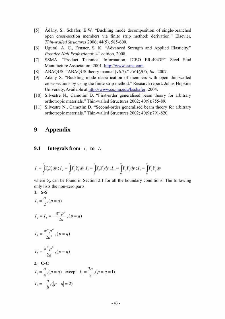
- 43 -

[5] Ádány, S., Schafer, B.W. “Buckling mode decomposition of single-branched open cross-section members via finite strip method: derivation.” Elsevier, Thin-walled Structures 2006; 44(5), 585-600.

[6] Ugural, A. C., Fenster, S. K. “Advanced Strength and Applied Elasticity.” Prentice Hall Professional; 4th edition, 2008.

[7] SSMA. “Product Technical Information, ICBO ER-4943P.” Steel Stud Manufacture Association; 2001. http://www.ssma.com.

[8] ABAQUS. “ABAQUS theory manual (v6.7).” ABAQUS, Inc. 2007. [9] Adany S. “Buckling mode classification of members with open thin-walled

cross-sections by using the finite strip method.” Research report. Johns Hopkins University, Available at http://www.ce.jhu.edu/bschafer; 2004.

[10] Silvestre N., Camotim D. “First-order generalised beam theory for arbitrary orthotropic materials.” Thin-walled Structures 2002; 40(9):755-89.

[11] Silvestre N., Camotim D. “Second-order generalised beam theory for arbitrary orthotropic materials.” Thin-walled Structures 2002; 40(9):791-820.

9 Appendix

9.1 Integrals from 1I to 5I

dyYYI q

a

p∫=0

1 ; dyYYI q

a

p∫=0

''2 dyYYI

q

a

p''

03 ∫= ; dyYYI

qp

a''

0

''4 ∫= ; dyYYI

qp

a'

0

'5 ∫=

where Yp can be found in Section 2.1 for all the boundary conditions. The following only lists the non-zero parts. 1. S-S

)(,21 qpaI ==

)(,2

22

32 qpapII =−==

π

)(,2 3

44

4 qpapI ==

π

)(,2

22

5 qpapI ==

π

2. C-C

)(,41 qpaI == except )1(,

83

1 === qpaI

)2(,81 =−−= qpaI

- 44 -

( ) )(,4

122

32 qpa

pII =+

−==π

( ) )2(,48

1 222

2 =−−+

= qpap

apI ππ and ( ) )2(,

481 222

2 −=−++

= qpap

apI ππ

( ) )2(,48

1 222

3 =−++

= qpaq

aqI ππ and ( ) )2(,

481 222

3 −=−−+

= qpaq

aqI ππ

( )[ ] )(,4

413

2224

4 qpa

ppI =++

=π

( ) ( ) )2(,8

113

224

4 =−+−

−= qpa

qpI π and ( ) ( ) )2(,8

113

224

4 −=−+−

−= qpa

pqI π

)(,4

)1( 22

5 qpa

pI =+

=π

)2(,8

)1(2

5 =−+

−= qpa

pqI π

3. S-C

)(,41 qpaI == except )1(,

83

1 === qpaI

)1(,2

)1(1 =−

+= qp

papI and )1(,

2)1(

1 −=−+

= qpq

aqI

( ) )(,1 22

32 qpapII =+

−==π

( ) )1(,2

12

2 =−+

−= qpa

ppI π and ( ) )1(,2

)1(1 22

2 −=−++

−= qpaq

qpI π

( ) )1(,2

)1(1 22

3 =−++

−= qpap

pqI π and ( ) )1(,2

12

3 −=−+

−= qpa

qqI π

( )[ ] )(,2

1)1(3

2224

4 qpa

pppI =+++

=π

( ) ( ) )1(,2

113

24

4 =−++

= qpa

qppI π and ( ) ( ) )1(,2

113

24

4 −=−++

= qpa

pqqI π

)(,)1( 22

5 qpapI =+

=π

- 45 -

)1(,2

)1)(1(2

5 =−++

= qpa

qpI π

4. C-G

)(,41 qpaI == except )1(,

83

1 === qpaI

)1(,81 =−−= qpaI

)(,4

41

21 2

2

32 qpa

p

II =⎥⎥⎦

⎤

⎢⎢⎣

⎡+⎟

⎠⎞

⎜⎝⎛ −

−==

π

)1(,8

21

8

41

21

2

22

2 =−⎟⎠⎞

⎜⎝⎛ −

−⎥⎥⎦

⎤

⎢⎢⎣

⎡+⎟

⎠⎞

⎜⎝⎛ −

= qpa

p

a

p

Iππ

and

)1(,8

21

8

41

21

2

22

2 −=−⎟⎠⎞

⎜⎝⎛ −

+⎥⎥⎦

⎤

⎢⎢⎣

⎡+⎟

⎠⎞

⎜⎝⎛ −

= qpa

p

a

p

Iππ

)1(,8

21

8

41

21

2

22

3 =−⎟⎠⎞

⎜⎝⎛ −

+⎥⎥⎦

⎤

⎢⎢⎣

⎡+⎟

⎠⎞

⎜⎝⎛ −

= qpa

q

a

q

Iππ

and

)1(,8

21

8

41

21

2

22

3 −=−⎟⎠⎞

⎜⎝⎛ −

−⎥⎥⎦

⎤

⎢⎢⎣

⎡+⎟

⎠⎞

⎜⎝⎛ −

= qpa

q

a

q

Iππ

)(,4

21

4

41

21

3

24

3

224

4 qpa

p

a

p

I =⎟⎠⎞

⎜⎝⎛ −

+⎥⎥⎦

⎤

⎢⎢⎣

⎡+⎟

⎠⎞

⎜⎝⎛ −

=ππ

)1(,8 3

44

4 =−−= qpaqI π and )1(,

8 3

44

4 −=−−= qpapI π

)(,164

)21( 2

22

5 qpaa

pI =+

−=

ππ

)1(,8

22

5 =−−= qpaqI π and )1(,

8

22

5 −=−−= qpapI π

5. C-F

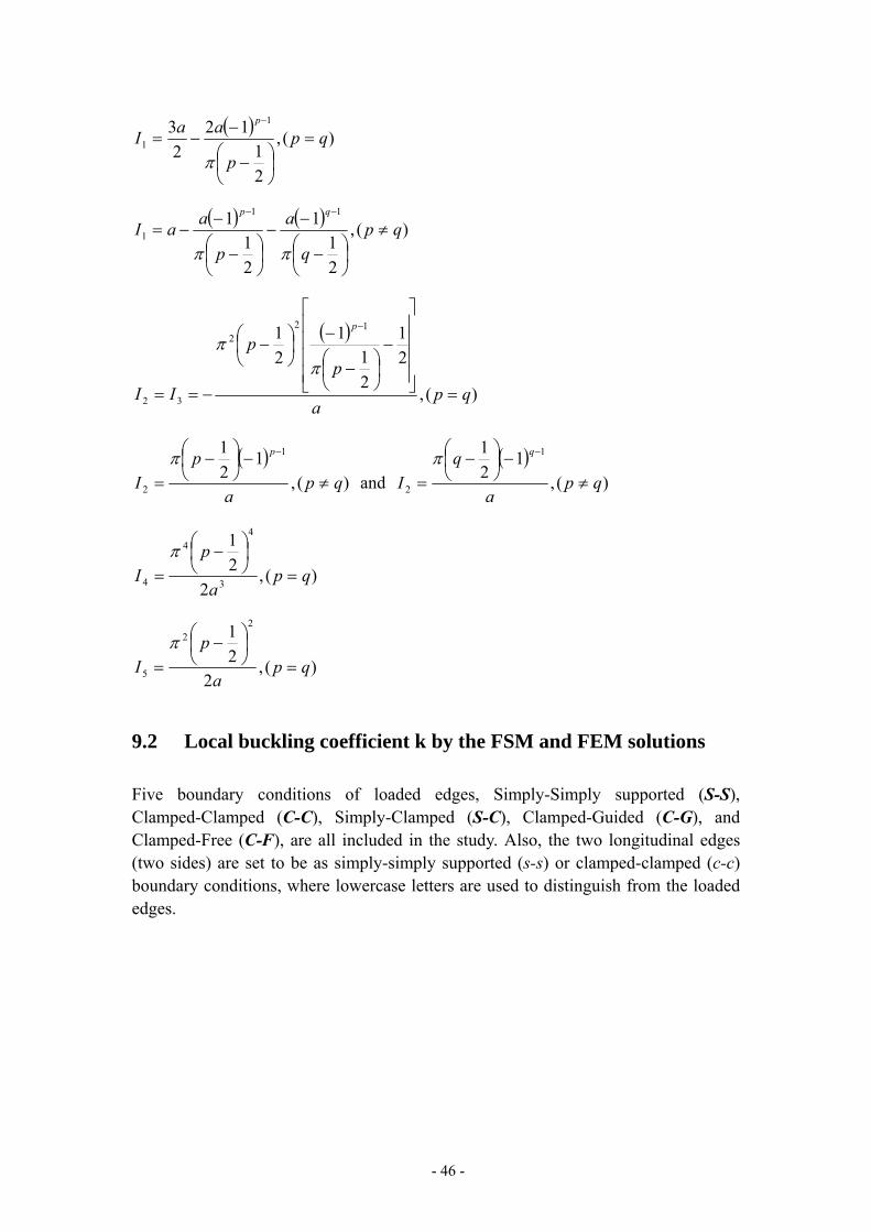
- 46 -

( ) )(,

21

122

3 1

1 qpp

aaIp

=⎟⎠⎞

⎜⎝⎛ −

−−=

−

π

( ) ( ) )(,

21

1

21

1 11

1 qpq

a

p

aaIqp

≠⎟⎠⎞

⎜⎝⎛ −

−−

⎟⎠⎞

⎜⎝⎛ −

−−=

−−

ππ

( )

)(,

21

21

121 12

2

32 qpa

pp

II

p

=⎥⎥⎥⎥

⎦

⎤

⎢⎢⎢⎢

⎣

⎡

−⎟⎠⎞

⎜⎝⎛ −

−⎟⎠⎞

⎜⎝⎛ −

−==

−

ππ

( ))(,

121 1

2 qpa

pI

p

≠−⎟

⎠⎞

⎜⎝⎛ −

=

−π and

( ))(,

121 1

2 qpa

qI

q

≠−⎟

⎠⎞

⎜⎝⎛ −

=

−π

)(,2

21

3

44

4 qpa

pI =

⎟⎠⎞

⎜⎝⎛ −

=π

)(,2

21 2

2

5 qpa

pI =

⎟⎠⎞

⎜⎝⎛ −

=π

9.2 Local buckling coefficient k by the FSM and FEM solutions

Five boundary conditions of loaded edges, Simply-Simply supported (S-S), Clamped-Clamped (C-C), Simply-Clamped (S-C), Clamped-Guided (C-G), and Clamped-Free (C-F), are all included in the study. Also, the two longitudinal edges (two sides) are set to be as simply-simply supported (s-s) or clamped-clamped (c-c) boundary conditions, where lowercase letters are used to distinguish from the loaded edges.

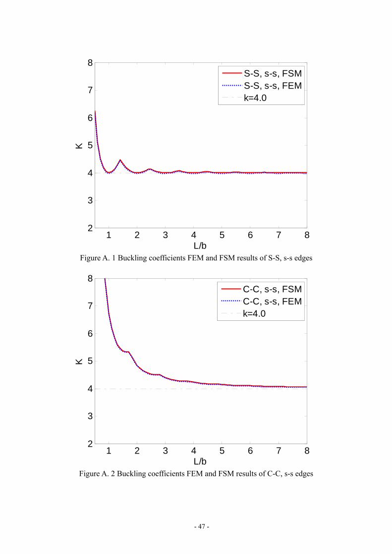
- 47 -

1 2 3 4 5 6 7 82

3

4

5

6

7

8

L/b

K

S-S, s-s, FSMS-S, s-s, FEMk=4.0

Figure A. 1 Buckling coefficients FEM and FSM results of S-S, s-s edges

1 2 3 4 5 6 7 82

3

4

5

6

7

8

L/b

K

C-C, s-s, FSMC-C, s-s, FEMk=4.0

Figure A. 2 Buckling coefficients FEM and FSM results of C-C, s-s edges

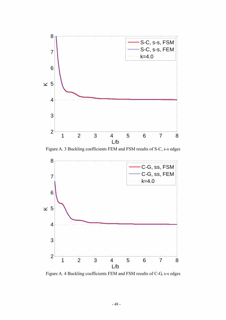
- 48 -

1 2 3 4 5 6 7 82

3

4

5

6

7

8

L/b

K

S-C, s-s, FSMS-C, s-s, FEMk=4.0

Figure A. 3 Buckling coefficients FEM and FSM results of S-C, s-s edges

1 2 3 4 5 6 7 82

3

4

5

6

7

8

L/b

K

C-G, ss, FSMC-G, ss, FEMk=4.0

Figure A. 4 Buckling coefficients FEM and FSM results of C-G, s-s edges

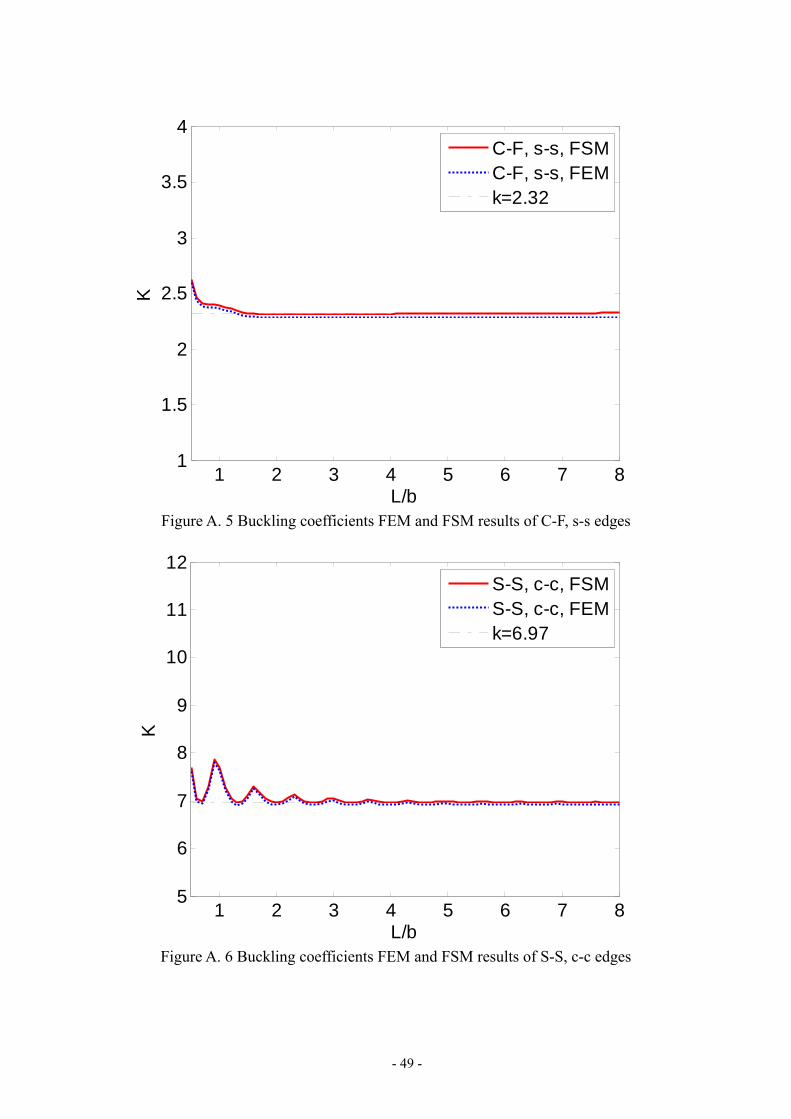
- 49 -

1 2 3 4 5 6 7 81

1.5

2

2.5

3

3.5

4

L/b

K

C-F, s-s, FSMC-F, s-s, FEMk=2.32

Figure A. 5 Buckling coefficients FEM and FSM results of C-F, s-s edges

1 2 3 4 5 6 7 85

6

7

8

9

10

11

12

L/b

K

S-S, c-c, FSMS-S, c-c, FEMk=6.97

Figure A. 6 Buckling coefficients FEM and FSM results of S-S, c-c edges

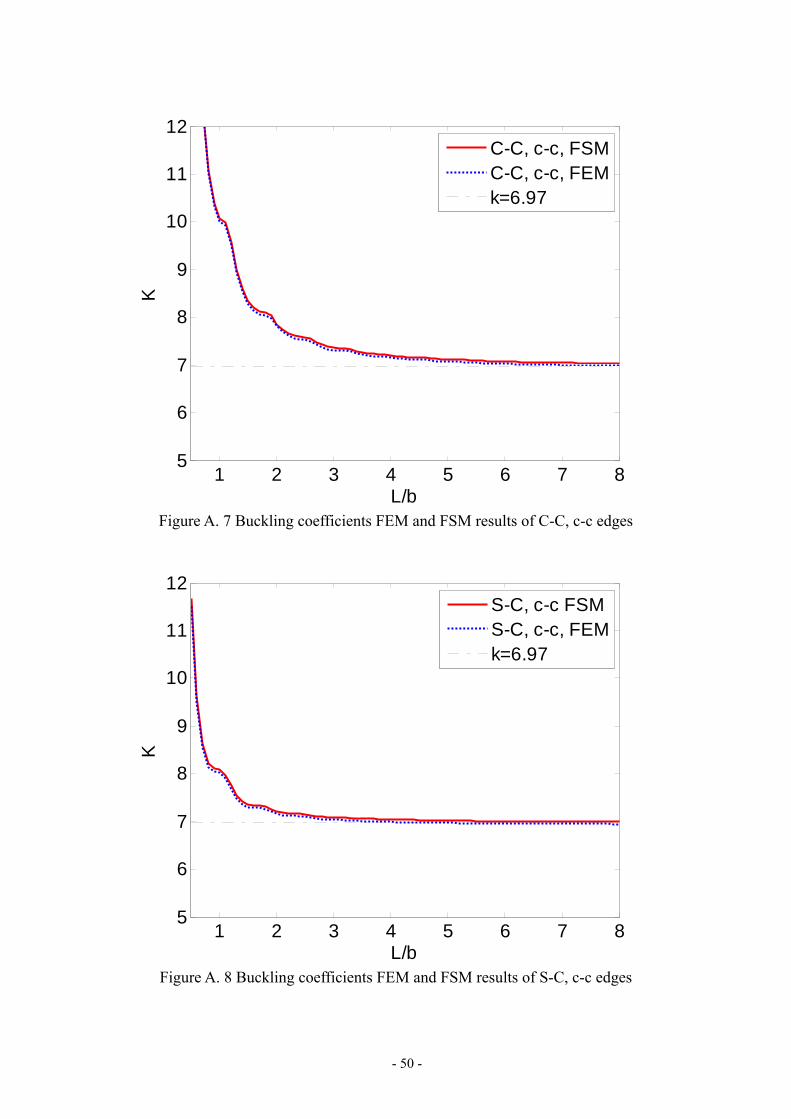
- 50 -

1 2 3 4 5 6 7 85

6

7

8

9

10

11

12

L/b

K

C-C, c-c, FSMC-C, c-c, FEMk=6.97

Figure A. 7 Buckling coefficients FEM and FSM results of C-C, c-c edges

1 2 3 4 5 6 7 85

6

7

8

9

10

11

12

L/b

K

S-C, c-c FSMS-C, c-c, FEMk=6.97

Figure A. 8 Buckling coefficients FEM and FSM results of S-C, c-c edges

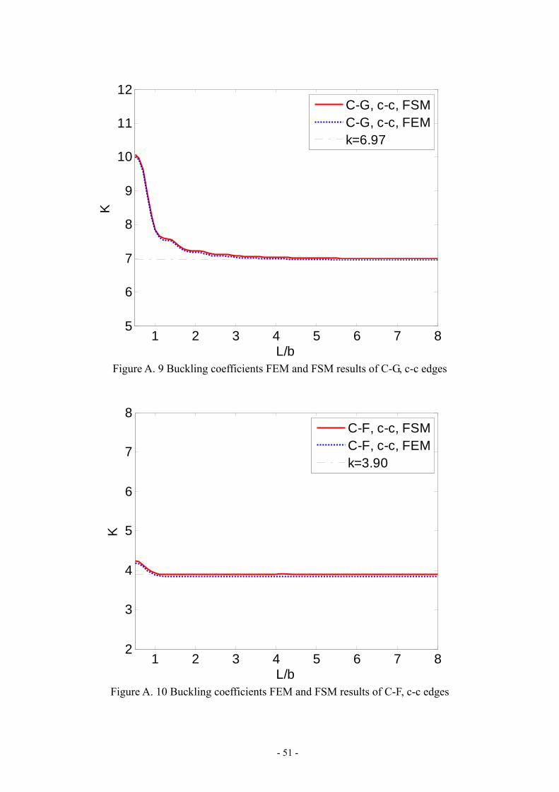
- 51 -

1 2 3 4 5 6 7 85

6

7

8

9

10

11

12

L/b

K

C-G, c-c, FSMC-G, c-c, FEMk=6.97

Figure A. 9 Buckling coefficients FEM and FSM results of C-G, c-c edges

1 2 3 4 5 6 7 82

3

4

5

6

7

8

L/b

K

C-F, c-c, FSMC-F, c-c, FEMk=3.90

Figure A. 10 Buckling coefficients FEM and FSM results of C-F, c-c edges