Finite Strip Analysis 1 local distortional later-torsional length of a half sine wave buckling...

1

Finite Strip Analysis

local distortional later-torsional

length of a half sine wave

buck

ling

mul

tiplie

r (s

tres

s, lo

ad,

or m

omen

t)

Finite Strip Analysisand the Beginnings of the Direct Strength Method

Toronto, July 2000

AISI Committee on Specifications

2


Overview

• Introduction• Background• A simple verification problem• Analyze a typical section

• Interpreting results (k, fcr, Pcr, Mcr)

• Direct Strength Prediction• Improve a typical section• Individual analysis - “do it yourself”

3


Introduction

• Understanding elastic buckling (stress, modes, etc.) is fundamental to understanding the behavior and design of thin-walled structures.

• Thorough treatment of plate buckling separates design of cold-formed steel structures from typical structures.

• Hand solutions for plate buckling have taken us a great distance but more modern approaches may be utilized now.

• Finite strip analysis is one efficient method for calculating elastic buckling behavior.

4


Introduction

• No new theory: Finite strip analysis uses the same “thin plate” theory employed in classical plate buckling solutions (e.g., k = 4) already in current use.

• Organized: The nuts and bolts of the analysis is organized in a manner similar to the stiffness method for frames and thus familiar to a growing group of engineers.

• Efficient: Single solutions and parameter studies can be performed on PCs

• Free: Source code and programs for the finite strip analysis is free

5


Introduction

finite element finite strip

6


What has to be defined?

nodesgive node numbergive coordinatesindicate if any additional support exist along the longitudinal edgegive applied stress on node

elementsgive element numbergive nodes that form the stripgive thickness of the strip

propertygive E, G, and v

lengthsgive all the lengths that elastic buckling should be examined at

7


Finite Strip Software

• CU-FSM– Matlab based full graphical version

– DOS engine only (execufsm.exe)

• Helen Chen has written a Windows front end “procefsm.exe” which uses the CU-FSM DOS engine (Thanks Helen!)

• Other programs with finite strip capability– THINWALL from University of Sydney

– CFS available from Bob Glauz

8


Overview




9


Theoretical Background

• Elastic buckling in matrix form

• Initial elastic stiffness [K]– specialized shape functions

• Geometric stiffness [Kg]

• Forming the solution

• Elastic buckling solution

10


Elastic Buckling (Matrix form)• standard initial elastic

stiffness form

• consider effect of stress on stiffness

• consider linear multiples of constant stress (f1)

• eigenvalue problem gives solution

dKF

dfKKF g

dfKKF 1g

dKdK g

11


What is [K]?

x

y

z

u1

v1

w1

1u2

v2

w2

a

b

2

2

1

1

2

2

1

1

w

w

v

u

v

u

w

w

v

u

v

u

w

0000

0000

0000

00000000

0000

0000

0000

uv

M

F

M

F

F

F

F

F

K

K

2

2

1

1

2

2

1

1

dKF

• [K] is the initial elastic stiffness

12


Shape Functions

m2

1 Yu

u

b

x

b

x1u

'm

2

1 Ym

a

v

v

b

x

b

x1v

a

ymsinYm

2

2

1

1

2

2

3

3

2

2

2

2

3

3

2

2

m w

w

b

x

b

xx

b

x2

b

x3

b

x

b

x21x

b

x2

b

x31Yw

x

y

z

u1

v1

w1

1u2

v2

w2

a

b

these shape functions arealso known as [N]

13


Strain-Displacement and [K] dABDBtK T

dN

v

u

v

u

Nv

u

2

2

1

1

d'NdB

xvyu

yv

xu

xy

y

x

d'NdB

yx

wy

wx

w

2

2

2

2

2

Plane stress Kuv comesfrom these strain-displacement relations

dNw

w

Nw

2

2

1

1

Bending Kw comesfrom these strain-displacement relations

14


Plane Stress Initial Stiffness

b2

aG

6

Eabk

4

Gak

4

Eak

b2

aG

12

Eabk

4

Gak

4

Eak

6

Gabk

b2

aE

4

Gak

4

Eak

12

Gabk

b2

aE

b2

aG

6

Eabk

4

Gak

4

Eak

symmetric6

Gabk

b2

aE

tK

22mm2xm2

2mm2xm

2m1m2xm

2

1

22mm2xm

2m1

uvm

where: km

am EEx

xy11 EEy

xy21

2

2

1

1

2

2

1

1

w

w

v

u

v

u

w

w

v

u

v

u

w

0000

0000

0000

00000000

0000

0000

0000

uv

M

F

M

F

F

F

F

F

K

K

2

2

1

1

2

2

1

1

15


Bending Initial Stiffness

x12m

xy2my

4m

3

x212m

xy2my

4m

2

x12m

xy2my

4m

3

x212m

xy2my

4m

2

x312m

xy2my

4m

x212m

xy2my

4m

2

x312m

xy2my

4m

x12m

xy2my

4m

3

y4m

2

x2

xy2m1

2m

x312m

xy2my

4m

w

Db

a2Dk

15

ab2

Dk15

ab4Dk

210

ab

Db

a3Dk

5

a3

Dk5

aDk

420

ab11

Db

aDk

30

ab

Dk15

abDk

840

ab3

Db

a3Dk

10

a

Dk5

aDk

840

ab13

Db

a6Dk

b5

a6

Dkb5

a12Dk

70

ab13

Db

a3Dk

10

a

Dk5

aDk

840

ab13

Db

a6Dk

b5

a6

Dkb5

a12Dk

140

ab9

Db

a2Dk

15

ab2

Dk15

ab4Dk

210

ab

Dk420

ab11D

b

a3

Dk5

aDk

5

a3

symmetric

Db

a6Dk

b5

a6

Dkb5

a12Dk

70

ab13

K

2

2

1

1

2

2

1

1

w

w

v

u

v

u

w

w

v

u

v

u

w

0000

0000

0000

00000000

0000

0000

0000

uv

M

F

M

F

F

F

F

F

K

K

2

2

1

1

2

2

1

1

16


• [Kg] is the stress dependent geometric stiffness, (compressive stresses erode stiffness) The terms may be derived through– consideration of the total potential energy due to in-plane

forces, or– equivalently consider equilibrium in the deformed geometry,

(i.e., consider the moments that develop in the deformed geometry due to forces which are in-plane in the undeformed geometry), also

– one can consider Kg as a direct manifestation of higher order strain terms.

What is [Kg]?

17


Developing [Kg]The tractions correspond to linear edge stresses f1 and f2 via T1 = f1t and T2 = f2t.

x

y

z

a

T T1

2

a

0

b

0

T211g dxdyGG

b

xTTTK

dGy

w

y

v

y

uT

where {d} is the nodal displacementsthe same shape functions as before are used,therefore [G] is determined through partial differentiation of [N].

18


Geometric Stiffness

212

2121

212

21212

21212121

21

21

2121

2121

g

T5T3b

T15T7b2T10T324symmetric

TTb3T7T6b2T3T5b

T6T7b2TT54T7T15b2T9T308

0000T3T70

00000T3T70

0000TT700TT370

00000TT700TT370

CK

a1680mbC 2

2

2

1

1

2

2

1

1

w

w

v

u

v

u

w

w

v

u

v

u

w

0000

0000

0000

00000000

0000

0000

0000

uv

M

F

M

F

F

F

F

F

K

K

2

2

1

1

2

2

1

1

19


• The stiffness matrix for the member is formed by summing the element stiffness matrices (this is done in exactly the same manner as the stiffness solution for frame analysis)– generate stiffness matrices in local coordinates

– transform to global coordinates ([k]n=Tk’

– add contribution of each strip to global stiffness, symbolically:

Forming the Complete Solution

strips#

1nnkK

strips#

1nngg kK

20


Eigenvalue Solution

ddKK

or

dKdK

1g

g

• The solution yields– the multiplier which gives the buckling stress– {d} the buckling mode shapes

• The solution is performed for all lengths of interest to develop a complete picture of the elastic buckling behavior

21


Overview




22


A Simple Verification Problem

• Find the elastic buckling stress of a simply supported plate using finite strip analysis.

SS

SS

SS SS

width = 6 in. (152 mm)thickness = 0.06 in. (1.52 mm)E = 29500 ksi (203000 MPa)v = 0.3

2

2

2

cr b

t

112

Ekf

2

2

2

cr ___

___

___112

________f

Hand Solution:

= 10.665 ksi

23


Finite Strip Analysis Notes(analysis of SS plate)

• double click procefsm.exe

• enter elastic properties into the box

• enter the node number, x coordinate, z coordinate, and applied stress– 1,0.0,0.0,1.0 which means node 1 at 0,0 with a stress of 1.0

– 2,6.0,0.0,1.0 which means node 2 at 6,0 with a stress of 1.0

• enter the element number, starting node number, ending node number, number of strips between the nodes (at least 2 typically 4 or more) and the thickness

– 1,1,2,2,0.06 which means element 1 goes from node 1 to 2, put 2 strips in there and t=0.06

• select plot cross-section to see the plate

• enter a member length (say 6) and number of different half wavelengths (say 10)

• do File - Save As - plate.inp

• now select view/revise raw data file

24


Finite Strip Analysis Notes(analysis of SS plate) continued

• View/Revise Raw Data File shows the actual text file that is used by the finite strip analysis program. All detailed modifications must be made here before completing the analysis. The format of the file is summarized as:

• The x, y, z, degrees of freedom are shown in the stripto the right.

• Supported degrees of freedom are supported along theentire length (edge) of the strip. The ends of the stripare simply supported (due to the selected shapefunctions). Set a DOF variable to 0 to support that DOF along the edge

#nodes #elements #lengthsEx Ey x y Gnode# xcoordinate zcoordinate xDOF zDOF yDOF DOF stress[repeat until all nodes are defined].element# nodei nodej t[repeat until all elements are defined].len1 len2 . . .[enter a total of #lengths lengths]

x

y

z

u1

v1

w1

1u2

v2

w2

a

b

25


Finite Strip Analysis Notes(analysis of SS plate) continued

• First modify degrees of freedom so the plate is simply supported along the long edges (the loaded edges are always simply supported). Put a pin along the left edge and a roller along the right edge.

– 1 0 0 1 1 1 1 1.0 becomes 1 0 0 0 0 1 1 1.0

– 2 3 0 1 1 1 1 1.0 stays the same

– 3 6 0 1 1 1 1 1.0 becomes 1 6 0 1 0 1 1 1.0

• Now delete the last line and replace it with the specific lengths that you want to use, say for instance “3 4 5 6 7 8”

• Now change the #lengths listed in the thrid column of the first line of the file to match the selected number, in this example we have 6 different lengths

• Now select Save for Finite Strip Analysis and save under the name plate.txt• Select Analysis - Open• Then type ‘plate.txt’ for the input file and ‘plate.out’ for the output file• Select Output - then plate.out - and open• Select Plot curve and plot mode, the result of this example is 10.69 ksi (vs. 10.665 ksi hand

solution - repeat using 4 strips - then result is 10.666 ksi)

26


Overview




27


Analyze a typical section

• Pure bending of a C– Quickie hand analysis

– Finite strip analysis using procefsm.exe

– Discussion

• Pure compression of a C– Quickie hand analysis

– Finite strip analysis

– Discussion

• Comparisons and Further Discussion

28


Strong Axis Bending of a C• Approximate the buckling stress for pure bending.

8.44

2.44

0.84

0.059 2

2

2

cr b

t

112

Ekf

3.0

ksi29500E

2

2

2

cr ___

___

___112

________f

2

2

2

cr ___

___

___112

________f

comp. lip

comp. flange

web

2

2

2

cr ___

___

___112

________f

29


Strong Axis Bending of a C• Approximate the buckling stress for pure bending.

8.44

2.44

0.84

0.059 2

2

2

cr b

t

112

Ekf

3.0

ksi29500E

ksi3.3144.8

059.0

3.0112

2950024f

2

2

2

cr

ksi4.6244.2

059.0

3.0112

295004f

2

2

2*

cr

lip

flange

web

ksi6.5684.0

059.0

3.0112

2950043.0f

2

2

2

cr

* this k value would be fine-tuned by AISI B4.2

30


Finite Strip Analysis Steps (strong axis bending of a C)

• Double click on procefsm.exe

• Select File - Open - C.inp

• Plot Cross Section

• View/Revise Raw Data File

• Go to bottom of text file and change lengths to “1 2 3 4 5 6 7 8 9 10 20 30 40 50 60 70 80 90 100”

• Go to top of file (1st line 3rd entry) change the number of lengths from 20 to 19

• Save for finite strip analysis as C.txt

• Select Analysis - Open - execufsm

• Enter in DOS window ‘C.txt’ return then ‘C.out’

• Select output - ‘C.out’ - open

• Check 2D, Check undef, push plot mode button

• Push plot curve, set half wave-length to 5 rehit plot mode, set to 30 and plot

• local buckling at 40ksi (~5 in. 1/2wvlngth), dist buckling at 52ksi (~30 in. 1/2wvlngth)

31


local buckling

half-wavelengthbuckling multiplier

local

distortional

32


distortional

33


Discussion

• Finite strip analysis identifies three distinct modes: local, distortional, lateral-torsional

• The lowest multiplier for “each mode” is of interest. The mode will “repeat itself” at this half-wavelength in longer members

• Higher multipliers of the same mode are not of interest.

• The meaning of the“half-wavelength” can bereadily understood fromthe 3D plot. For example:

34


Discussion

• How do I tell different modes?– wavelength: local buckling should occur at wavelengths near or

below the width of the elements, longer wavelengths indicate a different mode of behavior

– mode shape: in local buckling, nodes at fold lines should rotate only, if they are translating then the local mode is breaking down

• What if more minimums occur?– as you add stiffeners and other details more minima may occur,

every fold line in the plate adds the possibility of new modes. Definitions of local and distortional buckling are not as well defined in these situations. Use wavelength of the mode to help you decide.

35


Compression of a C• Approximate the buckling stress for pure

compression.8.44

2.44

0.84

0.059 2

2

2

cr b

t

112

Ekf

3.0

ksi29500E

ksi2.544.8

059.0

3.0112

295004f

2

2

2

cr

ksi4.6244.2

059.0

3.0112

295004f

2

2

2*

cr

lip

flange

web

ksi6.5684.0

059.0

3.0112

2950043.0f

2

2

2

cr

* this k value would be fine-tuned by AISI B4.2

36


Finite Strip Analysis Steps (compression of a C)

• Double click on procefsm.exe

• Select File - Open - C.inp

• Change all applied stress to compression +1.0

• Plot Cross Section

• View/Revise Raw Data File

• Go to bottom of text file and change lengths to “1 2 3 4 5 6 7 8 9 10 20 30 40 50”

• Go to top of file (1st line 3rd entry) change the number of lengths from 20 to 14

• Save for finite strip analysis as C.txt

• Select Analysis - Open - execufsm

• Enter in DOS window ‘C.txt’ return then ‘C.out’

• Select output - ‘C.out’ - open

• Check 2D, Check undef, push plot mode button

• Push plot curve, set half wave-length to 6 and rehit plot mode

• local buckling at 7.5ksi (pure compression)

37


Finite Strip AnalysisCompression of a C

• fcr local = 7.5 ksi

• fcr distortional ~ 20 ksi (this value may be fine tuned by selecting more lengths and re-analyzing)

• fcr overall at 80 in. = 29 ksi

38


Comparision of Elastic Results

• Hand Analysis– compression lip=56.6 flange=62.4 web=5.2

ksi– bending lip=56.6 flange=62.4 web=31.3 ksi

• Finite strip analysis– compression local=7.5 distortional~20ksi – bending local=40 distortional=52 ksi

39


Comparision of Results for Buckling Stress of a C

• Hand Analysis– Compression

• Lip = 56.6 ksi

• Flange = 62.4

• Web = 5.2

– Bending

• Lip = 56.6

• Flange = 62.4

• Web = 31.3

• Finite strip analysis– Compression

• Local = 7.5 ksi

• Distortional ~ 20

– Bending

• Local = 40

• Distortional = 52

40


Overview




41


Converting the results

• If f1 is the applied stress in the finite strip analysis and the multiplier that results from the elastic buckling thenfcr = f1 is known. How do we get k? Pcr? Mcr?

• k is found viawhere:b = element width of interest (flange, web, lip etc.)

• Pcr = Agfcr

• Mcr = Sgfcr (as long as f1 is the extreme fiber stress of interest)

2

2

2cr

2

2

2

cr t

b

E

1f12k

b

t

112

Ekf

42


Converting the results - Example

• For the C in pure compression what does the finite strip analysis yield for the local buckling k of the web?

• For the flange?

• Solutions are different when you recognize the interaction!

75.5k

059.0

44.8

29500

3.015.712k

t

b

E

1f12k

2

2

2

2

2

2cr

48.0k

059.0

44.2

29500

3.015.712k

2

2

2

43



• For the C in compression what is the elastic critical local buckling load? distortional buckling load? overall?– From CU-FSM or hand calculation get the section properties

– (Pcr)local = Agfcr = 0.885in2*7.5ksi = 6.6 kips

– (Pcr)distortional = Agfcr = 0.885in2*20 ksi = 17.7 kips

– (Pcr)overall at 80 in. = Agfcr = 0.885in2*29 ksi = 25.7 kips

44



• For the C in bending what is the elastic critical local buckling moment? distortional buckling moment?– From CU-FSM or hand calculation get the section properties

– (Mcr)local = Sgfcr = 2.256in3*40 ksi = 90 in-kips

– (Mcr)distortional = Sgfcr = 2.256in3*52 ksi = 117 in-kips

45


How can I use this information?

• Known– local buckling load (Pcr)local from finite strip analysis

– distortional buckling load (Pcr)distortional from finite strip analysis

– overall or Euler buckling load (Pcr)Euler may be flexural, torsional, or flexural-torsional in the special case of Kx=Ky=Kt then we may use finite strip analysis results, in other cases hand calculations for overall buckling of a column are used

– yield load (Py) from hand calculation

• Unknown– design capacity Pn

• Methodology: Direct Strength Prediction

46


Overview




47


Direct Strength Prediction

• The idea behind Direct Strength prediction is that with (Pcr)local, (Pcr)distortional and (Pcr)Euler known an engineer should be able to calculate the capacity reliably and directly without effective width.

• Current work suggests the following approach for columns– Find the inelastic long column buckling load (Pne) using the AISC

column curves already in the AISI Specification– Check for local buckling using new curve (less conservative than

Winter) on the entire member with the max load limited to Pne

– Check for distortional buckling using Hancock’s curve (more conservative than Winter) with the max load limited to Pne

– Design strength is the minimum

48


Direct Strength for Columns(1) Find inelastic long column buckling load

Pne = yP658.02c for 5.1c and y2

c

P877.0

for c > 1.5

c= crey PP

Py = AgFy

Pcre = Minimum of the elastic column buckling load inflexural, torsional, or torsional-flexural buckling, see Chapter C

(2) Local buckling strength*

Pnl = Pne for 776.0l and ne

4.0

ne

crl

4.0

ne

crl PP

P

P

P15.01

for l > 0.776

l= crlnePP

Pcrl = Elastic local column buckling load

49


Direct Strength for Columns (cont.)(3) Distortional buckling strength*

Pnd = Pne for 561.0d and ne

6.0

ne

crd

6.0

ne

crd PP

P

P

P25.01

for d > 0.561

d= crdnePP

Pcrd = Elastic distortional column buckling load

*these calculations include long column interaction, to ignore this interaction replace Pne with Py

(4) Design CapacityPn = minimum of Pnl , Pnd = …(ASD) = …(LRFD)

50


Column Example

• Consider the lipped C we have been analyzing. Assume 50 ksi yield, L=80 in. and Kx=Ky=Kt=1.0

• From finite strip analysis we know:– Pcrl = 6.6 kips

– Pcrd = 17.7 kips

– Pcre = 25.7 kips

– also Py = Agfy = 0.885*50 = 44.25 kips

51


Column Example (cont.)(1) Find inelastic long column buckling load

c= creyPP =


c

P877.0

for c > 1.5

Pne =


l= crlne PP =


4.0

ne

crl

4.0

ne

crl PP

P

P

P15.01

for l > 0.776

Pnl =

Pcrl = 6.6 kipsPcrd = 17.7 kipsPcre = 25.7 kipsPy = 44.25 kips

52


Column Example (cont.)(3) Distortional buckling strength*

d= crdne PP =


6.0

ne

crd

6.0

ne

crd PP

P

P

P25.01

for d > 0.561

Pnd =


(4) Design CapacityPn = minimum of Pnl , Pnd = = …(ASD) = …(LRFD)


53


Column Example (cont.)(1) Find inelastic long column buckling load

c= creyPP = 1.31


c

P877.0

for c > 1.5

Pne = 21.58 kips


l= crlne PP = 1.81


4.0

ne

crl

4.0

ne

crl PP

P

P

P15.01

for l > 0.776

Pnl = 12.2 kips


54


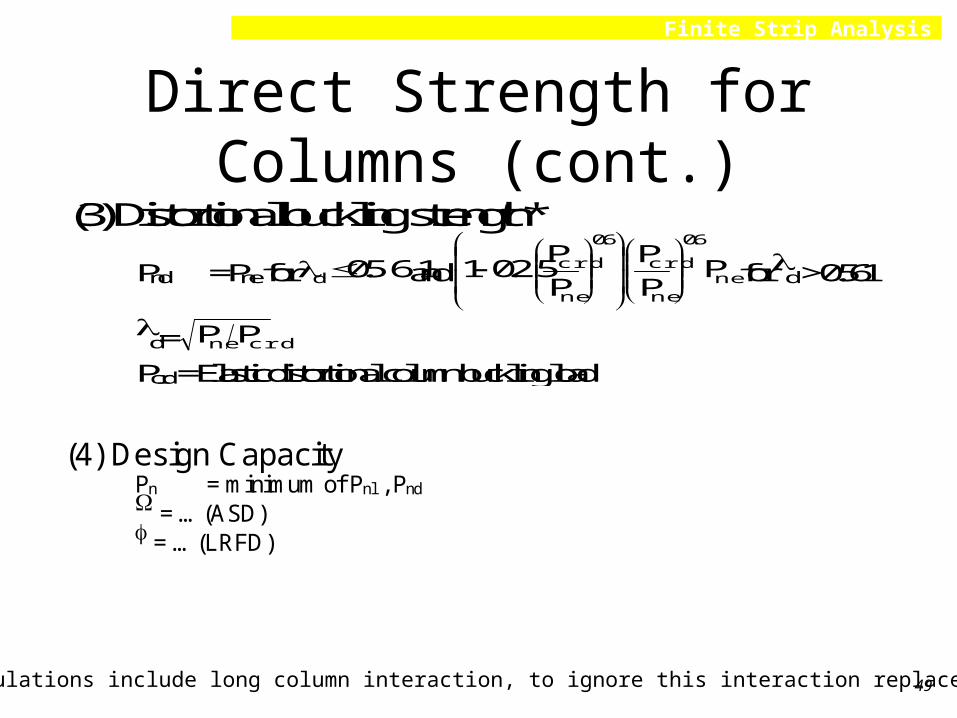
Column Example (cont.)(3) Distortional buckling strength*

d= crdne PP = 1.10


6.0

ne

crd

6.0

ne

crd PP

P

P

P25.01

for d > 0.561

Pnd = 14.9 kips


(4) Design CapacityPn = minimum of Pnl , Pnd = 12.2, 14.9 = 12.2 kips (local buckling limits) = …(ASD) = …(LRFD)

Pcrl = 6.6 kipsPcrd = 17.7 kipsPcre = 25.7 kipsPy = 44.25 kipsPne = 21.58 kips

55


Direct Strength for Beams

• Direct Strength prediction for beams follows the same format as for columns.– Find the inelastic lateral buckling load (Mne) using the strength curves

already in the AISI Specification– Check for local buckling using new curve (less conservative than Winter)

on the entire member with the max moment limited to Mne

– Check for distortional buckling using Hancock’s curve (more conservative than Winter) with the max moment limited to Mne

– Design strength is the minimum• Note, all the beams studied at this time have been laterally braced - therefore the

interaction between local and lateral buckling and distortional and lateral buckling has not been examined. For now, it is conservatively assumed that these modes can interact in the same manner as completed for columns. (This is what we do now when we use the effective section modulus)

56


Direct Strength for Beams(1) Find inelastic lateral buckling load

Mne = My if ycre M78.2M Mcre if ycre M56.0M and

= cre

y

M36

M10

y910 1M if 2.78My > Mcre > 0.56My

My = SgFy

Mcre = Elastic lateral buckling load of the beam


Mnl = Mne for 776.0l and ne

4.0

ne

crl

4.0

ne

crl MM

M

M

M15.01

for l > 0.776

l= crlne MM

Mcrl = Elastic local beam buckling moment

57


Direct Strength for Beams (cont.)(3) Distortional buckling strength*

Mnd = Mne for 561.0d and ne

6.0

ne

crd

6.0

ne

crd MM

M

M

M25.01

for d > 0.561

d= crdne MM

Mcrd = Elastic distortional beam buckling moment


(4) Design CapacityMn = minimum of Mnl , Mnd = …(ASD) = …(LRFD)

58


Beam Example

• Consider the lipped C we have been analyzing. Assume 50 ksi yield, assume the member is laterally braced, but distortional buckling is still free to form and thus a concern. Find the nominal capacity.

• From finite strip analysis we know:– Mcrl = 90 in-kips

– Mcrd = 117 in-kips

– Mcre = braced

– also My = Sgfy = 2.256*50 = 113 in-kips

59


Beam Example (cont.)(1) Find inelastic lateral buckling load

Mne = My if ycre M78.2M Mcre if ycre M56.0M and

= cre

y

M36

M10

y910 1M if 2.78My > Mcre > 0.56My

My = SgFy

Mcre = Elastic lateral buckling load of the beam


Mnl = Mne for 776.0l and ne

4.0

ne

crl

4.0

ne

crl MM

M

M

M15.01

for l > 0.776

l= crlne MM

Mcrl = Elastic local beam buckling moment

Mcrl = 90 in-kipsMcrd = 117 in-kipsMcre = bracedMy = 113 in-kips

Mne = My since “braced” = 113 in-kips

Mnl = 89 in-kips

60


Beam Example (cont.)(3) Distortional buckling strength*

Mnd = Mne for 561.0d and ne

6.0

ne

crd

6.0

ne

crd MM

M

M

M25.01

for d > 0.561

d= crdne MM

Mcrd = Elastic distortional beam buckling moment


(4) Design CapacityMn = minimum of Mnl , Mnd = …(ASD) = …(LRFD)

Mcrl = 90 in-kipsMcrd = 117 in-kipsMcre = bracedMy = 113 in-kips

Mnd = 86 in-kips

Mn = 86 in-kips, distortional controls even though elastic critical is 30% higher

61


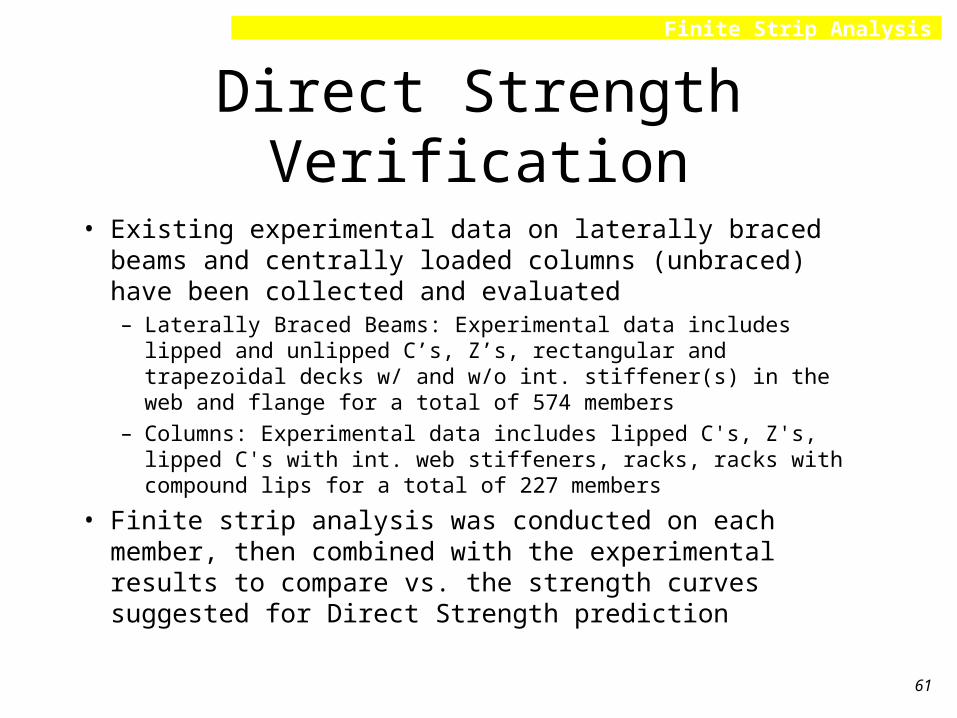
Direct Strength Verification

• Existing experimental data on laterally braced beams and centrally loaded columns (unbraced) have been collected and evaluated– Laterally Braced Beams: Experimental data includes lipped and

unlipped C’s, Z’s, rectangular and trapezoidal decks w/ and w/o int. stiffener(s) in the web and flange for a total of 574 members

– Columns: Experimental data includes lipped C's, Z's, lipped C's with int. web stiffeners, racks, racks with compound lips for a total of 227 members

• Finite strip analysis was conducted on each member, then combined with the experimental results to compare vs. the strength curves suggested for Direct Strength prediction

62


Laterally Braced Beams

0

0.5

1

1.5

0 1 2 3 4 5

Distortional

Local

Winter

Distortional Curve

Local Curve

max M My cr

M

Mtest

y

63


Columns

0 1 2 3 4 5 6 7 80

0.2

0.4

0.6

0.8

1

1.2

1.4

1.6

local buckling controlled

distortional buckling controlled

slenderness of controlling mode (Fn

/Fc r

).5

stre

ngth

F u/F

n

local strength curve

distortional strength curve

64


Direct Strength Verification (cont.)

• As the data shows, trends are clear, but large scatter can exist for a particular member.

• Using separate strength curves given herein for local and distortional limits– Laterally braced beams have test to predicted ratio of 1.14 for all

data, 1.05 for local limits and 1.16 for distortional limits

– Columns have test to predicted ratio of 1.01 for all data

• Preliminary calibration using the strength curves suggested herein appear to support the use of traditional =0.9 for beams and =0.85 for columns (presumably ASD factors would also remain unchanged)

65


Deflection Calculations

• Example strength & deflection calc. completed at fy

• Example strength & deflection calc. completed at fa

It is anticipated that degradation of gross properties (i.e, Ag Ig) due to local/distortional/overall buckling may be approximated in the same manner as the degradation in the strength, e.g.,

ygy fAP

yPP

ne PP crey658.0

nene

nl

ne

nlnl P

P

P

P

PP

4.04.0

15.01

)( yaaga fffAP

aPP

ne PP crea658.0

nene

nl

ne

nlnl P

P

P

P

PP

4.04.0

15.01

y

nlyeff f

PfatA ) (

a

nlaeff f

PfatA ) (

66


Limitations of Direct Strength

• Conservative solution when one element is extraordinarily slender (fcr approaches zero and the strength with it)

• Interaction of local-distortional-overall buckling not studied thoroughly for beams and deserves further study for columns

• Calibration of methods incomplete

• Impact of proposed changes incomplete

• Integration into existing design methods incomplete

• ...

67


Overview




68


Improve a Section

• Examine the results for the C section in compression that we previously evaluated

• Suggest alternative design

• Implement the design change

• Evaluate the finite strip results

• Recalculate the strength

69


Previous Results

70


Alternative Design Suggestions

• Intermediate stiffener in the web

• Multiple intermediate stiffeners in the web

• Decrease width of one flange in order to incorporate a small fold in the web so that sections could be nested together

• others...– ________________________– ________________________

71


Suggested Alternative

• Old • New

(2.44,0.84)

(2.44,0.0)(0.50,0.00)

(0.50,1.50)

(0.00,2.00)

(0.00,8.44) (2.44,8.44)

(2.44,7.60)

72


73


Convert stress to load

• For the C in compression what is the elastic critical local buckling load? distortional buckling load? overall?– From CU-FSM or hand calculation get the section properties

– (Pcr)local = Agfcr = 0.868in2*13.2ksi = 11.4 kips

– (Pcr)distortional = Agfcr = 0.868in2*28 ksi = 24.3 kips

– (Pcr)overall at 80 in. = Agfcr = 0.868in2*26 ksi = 22.6 kips

– Py for 50 ksi yield = Agfy = 0.868in2*50 ksi = 43.4 kips

74


Direct Strength(1) Find inelastic long column buckling loadc= creyPP = 1.38


c

P877.0

for c > 1.5

Pne = 19.4 kips


l= crlne PP = 1.30


4.0

ne

crl

4.0

ne

crl PP

P

P

P15.01

for l > 0.776

Pnl = 13.7 kips


75


Direct Strength (cont.)(3) Distortional buckling strength*

d= crdne PP = 0.89


6.0

ne

crd

6.0

ne

crd PP

P

P

P25.01

for d > 0.561

Pnd = 15.8 kips


(4) Design CapacityPn = minimum of Pnl , Pnd = 13.7, 15.8 = 13.7 kips (local buckling limits) = …(ASD) = …(LRFD)

Pcrl = 11.4 kipsPcrd = 24.3 kipsPcre = 22.6 kipsPy = 43.4 kipsPne = 19.4 kips

76


Comparison

• “typical” C• Pcrl = 6.6 kips

• Pcrd = 17.7 kips

• Pcre = 25.7 kips

• Py = 44.2 kips

• Pne = 21.6 kips

• Pnl = 12.2 kips

• Pnd = 14.9 kips

• Pn = 12.2 kips

• “nestable” C• Pcrl = 11.4 kips

• Pcrd = 24.3 kips

• Pcre = 22.6 kips

• Py = 43.4 kips

• Pne = 19.4 kips

• Pnl = 13.7 kips

• Pnd = 15.8 kips

• Pn = 13.7 kips

77


• Changing boundary conditions– eliminate a mode you are not interested in by temporarily supporting

a DOF

– use symmetry and anti-symmetry to examine different modes and behavior

– bound solutions by looking at fix vs. free conditions

Extras

78


Extras

• Adding an elastic support– you want to add elastic springs to the cross-section to model external

(continuous) support. This can be done only indirectly by adding an unloaded strip to your model

– The elastic stiffness kx, ky, kz and k of a single strip is given previously. Note selection of strip width, t, and boundary conditions will generate all 4 k’s currently no method is available for adding springs for only one DOF

79


Extras

2

2

1

1

2

2

1

1

w

w

v

u

v

u

w

w

v

u

v

u

w

0000

0000

0000

00000000

0000

0000

0000

uv

M

F

M

F

F

F

F

F

K

K

2

2

1

1

2

2

1

1

x

y

z

u1

v1

w1

1u2

v2

w2

a

b

defining a single unloaded strip fixed at the 1 edgeand attached at the 2 edge will add the above elasticstiffness to the solution wherever the 2 edge is attachedto the member. Remember, this stiffness is along thelength of the member (the length of the strip)

in order to make an unloaded strip you will have to createa very short dummy element near the 2 edge because loadingis defined at the nodes not the elements

00

00

12

80


Extras

• Assemblage– 2 C’s linked

togethervs. a singleC sectionresults arein bending.CU-FSMused foranalysis

81


Extras

• Beam-columns– load with the expected stress distribution

instead of doing separate beam and column analysis

– Make your own elastic buckling interaction curve for a particular shape

82


Extras

• Matlab version (free, but you need Matlab)– Robust graphical interface– Calculates section properties– Add P and M, or combinations thereof directly instead of

adding stress– Compare two analyses directly– Perform parametric studies– Completely free and available source, modify as you wish– Write your own programs and software that call any of the

finite strip routines

83


Limitations of Finite Strip• Elastic only: elastic buckling stress is useful, but it is

– not an allowable stress,– not necessarily the stress at which buckling “ensues”,– not a conservative design ultimate stress.

• Optimum design– Do not design so that the elastic buckling stress of all modes is at or near

the same stress - this invariably leads to coupled instabilities and should be avoided - note that different strength curves are used for different modes.

• Identification of minima– Certain members and certain loadings blur the distinctions between modes.

Exercise judgment and remain conservative when in doubt, i.e., the distortional buckling strength curve is more conservative than the local buckling curve.

84


Limitations of Finite Strip• Mixed wavelength modes

– Finite strip analysis can not identify situations when the wavelength in the flange differs from that in the web. Finite element analysis indicates this can happen in certain circumstances. Analysis to date shows that the finite strip formulation does not lead to undo errors, but further work needed.

• Point-wise bracing, punch-outs...– Any item that discretely varies along the length must be “smeared” in

the current approach. The benefit of individual braces is difficult to quantify. This is a practical limit not a theoretical limit of the current approach. For now, engineering judgment is required when evaluating bracing, punch-outs etc..

• Shear interaction

85


Overview




86


Geometry of Examples

8.44

2.44

0.059

C_nolip

8.44

2.44

0.84

0.059

C

15.93

3.43

0.97

0.068

C_deep

3.95

3.0

0.81

0.083

C_rack

4

4

0.060

L

4

4

0.25

0.060

L_lip

10.0

5.0 1.0

0.075

H

8.44

2.44

0.68@50o

0.059

Z

0.90@50o

11.93

2.06

0.070

Z_deepplate

6

drawings not to scale, all dim. in inches

87


END

88


Classical Derivation for k

• Classical methods tend to use an energy approach (following Timoshenko)– assume a series for deflected shape (must match boundary conditions)

– determine the internal strain energy (independent of loading)

– determine the external work (dependent on loading)

– form the total potential energy

– take the variation of the total potential energy with respect to the amplitude coefficients of the series and set to zero

– determine the desired number of terms to be used in the series

– calculate the buckling stress and k

89


Classical derivation for k (cont.)

m n

mn b

ynsin

a

xmsinaw

a

0

2

2

2

2

2b

0

2/t

2/t

22plate dxdy

y

w

x

wdzz

12

EU

b

0

a

0

2

121

plate dxdyx

w

b

y1tfW

plateplate WU

0amn

consider solution for a simply supported plate with a stress gradient

displaced shape

internal energy

external work

total potential energy

variation and solution

Finite Strip Analysis 1 local distortional later-torsional length of a half sine wave buckling...

Documents

Transcript of Finite Strip Analysis 1 local distortional later-torsional length of a half sine wave buckling...