Rene Schott, Laurent Alonso, Philippe Chassaing, Edward M. Reingold, Average-case Analysis of

International Journal of Mathematicsand Computer Science, 1(2006), 37-61

b b

MCS

Average-case Analysis of the Chip Problem

Laurent Alonso1, Philippe Chassaing2, Edward M. Reingold3 &

Rene Schott2

1 INRIA-Lorraine and LORIA, Universite Henri Poincare-Nancy IBP 239, 54506 Vandoeuvre-les-Nancy, France

e-mail: [email protected]

2 Institut Elie Cartan, Universite Henri Poincare-Nancy IBP 239, 54506 Vandœuvre-les-Nancy, France

e-mail: [email protected]; [email protected]

3 Department of Computer Science, Illinois Institute of TechnologyStuart Bldg, 10 W. 31st St., Suite 236, Chicago, Illinois 60616-2987 USA

e-mail: [email protected]

(Received August 2, 2005, Accepted September 19, 2005)

Abstract

In the system level, adaptive fault diagnosis problem we must determine whichcomponents (chips) in a system are defective, assuming the majority of themare good. Chips are tested as follows: Take two chips, say x and y, and havex report whether y is good or bad. If x is good, the answer is correct, but ifx is bad, the answer is unreliable and can be either wrong with probability αor right with probability 1 − α. The key to identifying all defective chips is toidentify a single good chip which can then be used to diagnose the other chips;the chip problem is to identify a single good chip. In [1] we have shown thatthe chip problem is closely related to a modified majority problem in the worst

case and have used this fact to obtain upper and lower bounds on algorithmsfor the chip problem. In this paper, we show the limits of this relationshipby showing that algorithms for the chip problem can violate lower bounds onaverage performance for the modified majority problem and we give an algorithmfor the “biased chip” problem (a chip is bad with probability p) whose averageperformance is better than the average cost of the best algorithm for the biasedmajority problem.

1 Introduction

In system diagnosis, according to [14], we consider

a system consisting of a set U of n units (processors, modules, etc.)at most t of which are faulty. An external observer wishes to identifythe faulty units. The observer acquires information by requestingthe results of certain tests performed by one unit upon another; e.g.,

Key words and phrases: Fault diagnosis, algorithm analysis, chip problem,majority problem, probabilistic algorithms.AMS (MOS) Subject Classifications: 68Q25, 68P10, 68Q20, 68M15ISSN 1814-0424 c© 2006, http://ijmcs.future-in-tech.netThis research was supported in part by INRIA and the NSF, through grant numbersNSF INT 90-16958 and 95-07248. Supported in part by NSF grants CCR-93-20577and CCR-95-30297 and by a Meyerhoff Visiting Professorship at the WeizmannInstitute of Science

38 L. Alonso, P. Chassaing, E. Reingold and R. Schott

ui ∈ U might be asked to determine if uj ∈ U is faulty or not. . . Ifui is fault-free then [the test performed by ui] is assumed reliable;if ui is faulty however, ui may find uj either faulty or fault-free,regardless of the actual condition of uj .

For example, suppose we have a combination of electronic components in aninaccessible location (in outer space, under the sea, in a deadly environmentsuch as a nuclear reactor, and so on). We are able to test components only atgreat expense, and only relative to other components—when we get test results,the testing components themselves may be faulty. We thus have a problem inwhich we get results such as “According to component x, component y is func-tioning properly” or “According to component x, component y is defective.” Itis a complex issue to determine which components are defective under such con-ditions; furthermore, since communication itself is difficult, we do not want toexpend unnecessary effort by asking more questions than the minimum numberneeded.For convenience of language we follow [7, exercise 4-7, page 75] and refer to“chips” rather than “units” or “components”. An algorithm can determinewhether a bad (faulty) chip exists if and only if a strict majority of the chipsare fault-free [12]. The basic problem is to determine that some chip is good(fault-free) so we can rely on its diagnosis of other chips; the difficulty is thata faulty chip can behave exactly like a fault-free one. However, there are con-figurations of test results in which the assumption that some particular chip xis bad implies that a majority of chips are faulty too—since we know that astrict majority are good, we are then sure that x is good, and we can rely onits diagnosis; Figure 1 shows just such a configuration. There are a number ofattendant algorithmic questions, including designing and analyzing algorithmsand determining lower bounds for a variety of problems. These problems havea long history and lengthy bibliography; Pelc and Upfal [11] give an excellentsummary with a useful bibliography. In this paper we address only the chip

problem—the question of finding a single good chip, assuming that the major-ity of the chips are good and that any chip can test any other. We considerboth the worst and average case for this problem, using results of the “majorityproblem” as starting point of our investigations.This paper is organized as follows. We begin with a brief section introducingthe necessary background of the majority problem. Then, in Section 4, we giveresults and conjectures about the average case under two different sets of proba-blistic assumptions. We conclude in Section 5 with some observations and openproblems.

2 Majority Problems

The majority problem of [2], [3], and [13] is to determine the majority color in aset of n elements {x1, x2, . . . , xn}, each element of which is colored either blueor red, by pairwise equal/not equal color comparisons. When n is even, we must

Average-case Analysis of the Chip Problem 39

S R H

T D I

A O J

F B K

G E C

Figure 1: Sample test configuration of fifteen chips. We show a link from onechip to another labeled by a smiling face if the chip at the base of the arrowdiagnoses the chip at the point of the arrow as good, and label the link with afrowning face if the diagnosis is bad. Chip F must be bad and chip A must begood by the following logic: If A were bad, chips D, T , and B would be badbecause each of them diagnoses A as good; then, similarly, chips R and C wouldhave to be bad, making the set {A,B,C,D,R, T} of six chips all bad. However,since I diagnoses O as bad, one of those two must be bad—O is bad if I is goodwhile I is bad if O is good—implying that one of H or K must also be bad.Thus if A were bad there would be at least eight bad chips, a majority of thechips.


report that there is no majority if there are equal numbers of each color. In theworst case, exactly

n − ν(n)

questions are necessary and sufficient for the majority problem, where, following[8], ν(n) is the number of 1-bits in the binary representation of n. This resultwas first proved by Saks and Werman [13]; [2] gave a short, elementary proof;[17] found yet a different approach. [3] proved that any algorithm that correctlydetermines the majority must on the average use at least

2n

3−

√

8n

9π+ Θ(1)

color comparisons, assuming all 2n distinct colorings of the n elements areequally probable. Furthermore, [3] describes an algorithm that uses an aver-age of

2n

3−

√

8n

9π+ O(log n)

color comparisons. Together these bounds imply that

2n

3−

√

8n

9π+ O(log n)

such comparisons are necessary and sufficient in the average case to solve theoriginal majority problem.The biased case of the majority problem has been investigated by Chassaing [6].Let p be the probability that an element is blue and q = 1 − p the probabilitythat it is red. Let ρ = q/p. Chassaing proved that

Φ(ρ)n + O(n12+ǫ)

comparisons are necessary and sufficient in the biased case of the majority prob-lem on n elements, where

Φ(ρ) =1 − ρ

4

∞∑

i=0

1 + ρ2i

2i(1 − ρ2i). (1)

Note that the function Φ is well defined for ρ = 1 since limρ→1 Φ(1) = 2/3; notefurther that Φ(0) = 1/2. Tedious computation shows that, as expected, Φ isincreasing in ρ.In the modified majority problem, we are guaranteed the existence of a strictmajority. For odd n, the original and modified problems are obviously identicaland bounds of the previous paragraphs apply directly to the modified major-ity problem. But when n is even, the modified problem is clearly no harderthan the original problem for n − 1 elements and may even be (a bit) sim-pler. Given algorithm M for the (2k − 1)-original-majority-problem, we solvethe (2k)-modified-majority-problem by removing one element and running al-gorithm M on the 2k−1 remaining elements—the answer is then obviously also


correct for the (2k)-modified-majority-problem. The other direction is open:Given algorithm M ′ for the (2k)-modified-majority-problem, can we apply it tothe (2k − 1)-original-majority-problem? If so it would prove that the modifiedproblem for 2k elements is no harder than the original problem for 2k − 1 el-ements and establish the worst-case lower bound of 2k − 1 − ν(2k − 1) colorcomparisons. We believe this lower bound is correct, but cannot prove it.

3 Happy Trees

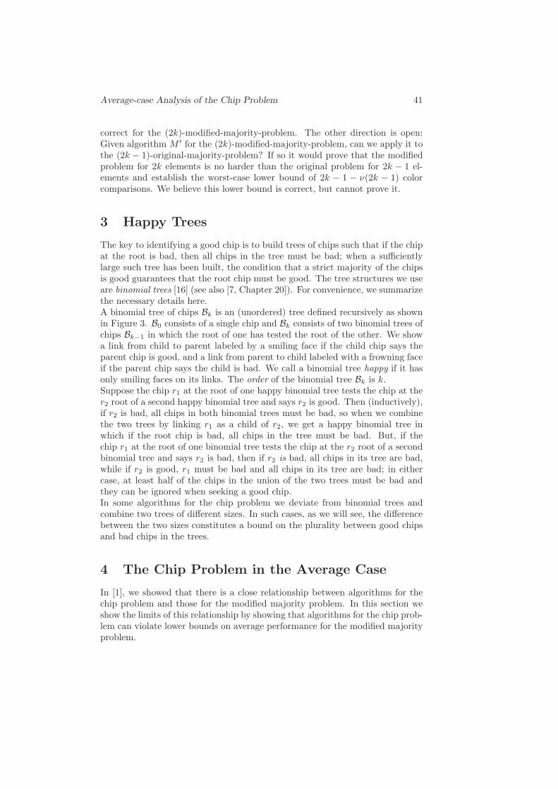
The key to identifying a good chip is to build trees of chips such that if the chipat the root is bad, then all chips in the tree must be bad; when a sufficientlylarge such tree has been built, the condition that a strict majority of the chipsis good guarantees that the root chip must be good. The tree structures we useare binomial trees [16] (see also [7, Chapter 20]). For convenience, we summarizethe necessary details here.A binomial tree of chips Bk is an (unordered) tree defined recursively as shownin Figure 3. B0 consists of a single chip and Bk consists of two binomial trees ofchips Bk−1 in which the root of one has tested the root of the other. We showa link from child to parent labeled by a smiling face if the child chip says theparent chip is good, and a link from parent to child labeled with a frowning faceif the parent chip says the child is bad. We call a binomial tree happy if it hasonly smiling faces on its links. The order of the binomial tree Bk is k.Suppose the chip r1 at the root of one happy binomial tree tests the chip at ther2 root of a second happy binomial tree and says r2 is good. Then (inductively),if r2 is bad, all chips in both binomial trees must be bad, so when we combinethe two trees by linking r1 as a child of r2, we get a happy binomial tree inwhich if the root chip is bad, all chips in the tree must be bad. But, if thechip r1 at the root of one binomial tree tests the chip at the r2 root of a secondbinomial tree and says r2 is bad, then if r2 is bad, all chips in its tree are bad,while if r2 is good, r1 must be bad and all chips in its tree are bad; in eithercase, at least half of the chips in the union of the two trees must be bad andthey can be ignored when seeking a good chip.In some algorithms for the chip problem we deviate from binomial trees andcombine two trees of different sizes. In such cases, as we will see, the differencebetween the two sizes constitutes a bound on the plurality between good chipsand bad chips in the trees.

4 The Chip Problem in the Average Case

In [1], we showed that there is a close relationship between algorithms for thechip problem and those for the modified majority problem. In this section weshow the limits of this relationship by showing that algorithms for the chip prob-lem can violate lower bounds on average performance for the modified majorityproblem.


B0 = Bk =S1

Bk−1

S2

Bk−1

Figure 2: Binomial trees of chips. The smiling face indicates the chip at thebase of the arrow says that the chip at the point of the arrow is good. If allarrows in the trees S1 and S2 are smiling and the chip at the root of S2 is bad,all chips in both S1 and S2 must be bad by induction. Since B0 contains a singlechip, Bk contains 2k chips.

Bk =

S1

Bk−1S2

Bk−1

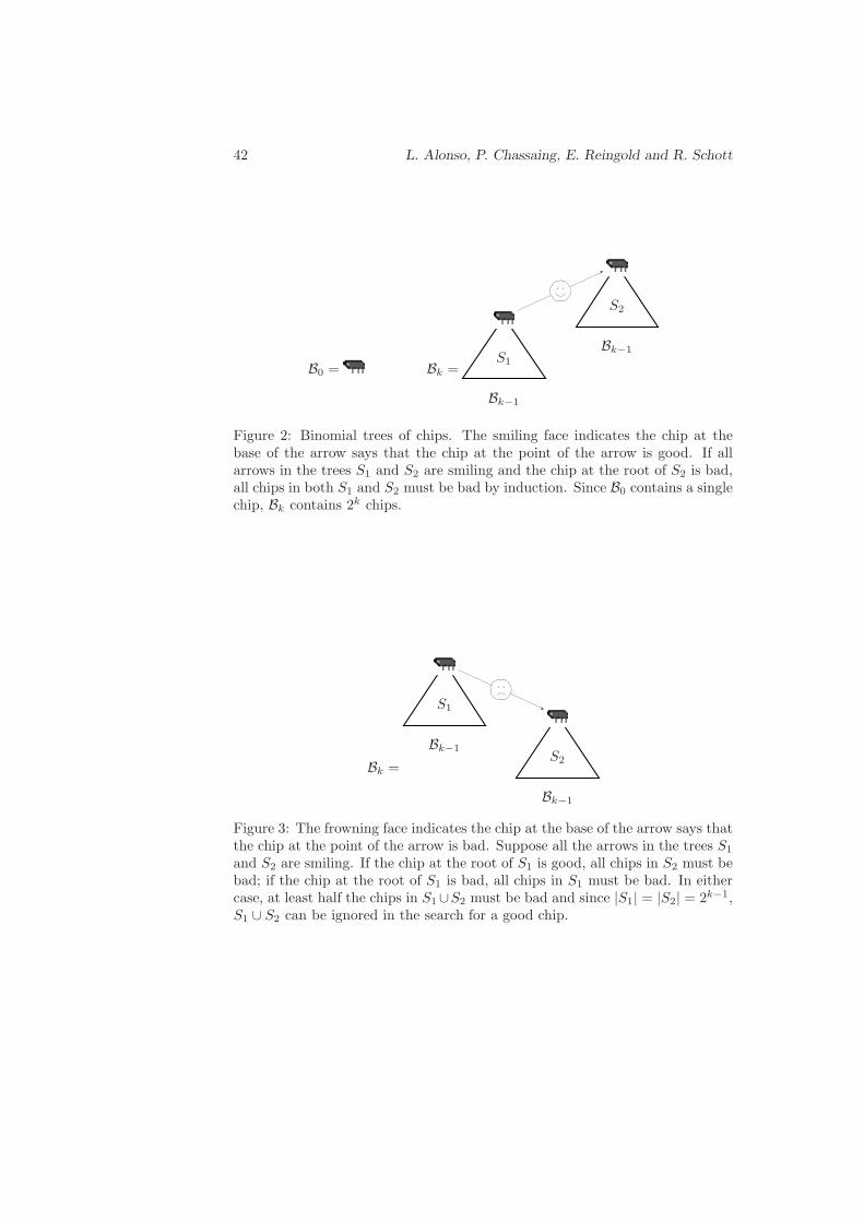
Figure 3: The frowning face indicates the chip at the base of the arrow says thatthe chip at the point of the arrow is bad. Suppose all the arrows in the trees S1

and S2 are smiling. If the chip at the root of S1 is good, all chips in S2 must bebad; if the chip at the root of S1 is bad, all chips in S1 must be bad. In eithercase, at least half the chips in S1∪S2 must be bad and since |S1| = |S2| = 2k−1,S1 ∪ S2 can be ignored in the search for a good chip.


4.1 The Model and Previous Results

We use a variant of the model of Pelc and Upfal [11], who consider that eachchip is good independently with known probability p and bad with probabilityq = 1−p < p; the number N of good chips thus has a binomial distribution. LetQ be the probability that an adaptive diagnosis algorithm incorrectly identifiesthe set of faulty chips. Pelc and Upfal prove that the minimal number of testsrequired to identify all faulty chips in the worst case is n + Θ(log 1

Q ). Thereare three main differences between their results and ours: we limit ourselves toalgorithms that never fail; we study the average number of tests required; andwe focus on the problem of finding a single good chip, assuming at most n − 1additional tests will be needed to determine the status of the n− 1 other chips.According to [12], a configuration with N ≤ n/2 good chips can fool any al-gorithm, but there do exist algorithms that reliably diagnose any configurationwith a strict majority of good chips. Thus in order for reliable algorithms toexist, we must preclude the possibility that N ≤ n/2, so we consider the modelof Pelc and Upfal with the additional condition that N > n/2; that is, we as-sume that each partition of the chips into k > n/2 good chips and n − k badchips has probability

pkqn−k

Pr(N > n/2). (2)

As we show in Proposition 2, this is only a slight change, since we have, forp > q,

Pr(N ≤ n/2) =∑

0≤k≤n/2

(

n

k

)

pkqn−k

≤ e−(p−q)2n/2, (3)

and hence the denominator of (2) is close to 1.The computation of the average cost of algorithms requires a probabilistic modelfor diagnosis of faulty chips; we use a simple instance of those surveyed in [10]:given a bad chip x and some other chip y, we assume that x lies about y withprobability α, and tells the truth with probability 1−α. We assume that p andα are known, but this in no way weakens the results since in the likely case thatp and α are unknown, we could obtain good approximations of them at costo(n), using statistics on a sample of n1−ε chips.Note that if we know that α = 0, no chip lies, and the problem has triviallyaverage cost O(1). However, in the setting where p and α are unknown butwhere α = 0, we will find any no erroneous diagnoses in our sample of n1−ε

chips; this would only tell us that α is quite small, not that α = 0. So, we couldnot assume that each diagnosis is reliable, and we could only rely on a majorityof chips being good; thus not knowing that α = 0 leads to a lower bound Θ(n)for the best average cost, not O(1).

Choosing Q = Pr(N ≤ n/2) in Pelc and Upfal [11] allows comparison oftheir results to ours. Using (3), their result translated to the problem of finding


(1,1,1,1,1)

(2,1,1,1)

(3,1,1) (1,1,1)

(2,1) (1)

(1,1,1)

(2,1) (1)

Figure 4: Optimal tree for n = 5 in the majority problem [3]. It has expectedcost 2.25.

a single good chip gives the trivial worst case bound of Θ(log 1Q ) = Θ(n). It

is equally easy to see that the minimal average cost is Θ(n). The problemwe address is much more difficult: determining the value of the multiplicativeconstant in Θ(n). Thus we have to design the algorithm more carefully than in[11].

4.2 The Unbiased Case

In the simple unbiased case, we ignore p and q and assume instead that a setof n good and bad chips is chosen at random so that each set of chips with amajority of good chips is equally probable. That is, each of the

∑

n/2<k≤n

(

nk

)

sets of n chips having a strict majority of good chips occurs with probability1/

∑

n/2<k≤n

(

nk

)

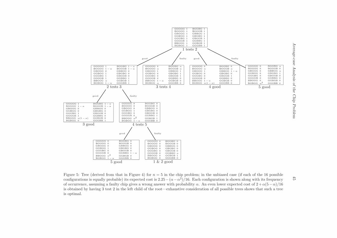
.Since the modified majority problem is identical to the original majority problemfor odd n, the tree in Figure 4 (which is derived from the algorithm describedin the conclusions of [3]), is optimal for the modified majority problem withn = 5, having cost 2.25. On the other hand, Figure 5 shows the identical treefor the chip problem with n = 5 having expected cost 2.25− (α−α2)/16 if eachof the 16 possible configurations is equally probable. Since (α − α2)/16 > 0 for0 < α < 1, this proves that the chip problem and the modified majority problemare not the same in the average case for 0 < α < 1. An even lower expected costof 2+α(5−α)/16 is obtained by having chip 3 test chip 2 in the left child of theroot in Figure 5; exhaustive consideration of all possible trees shows that sucha tree is the optimal way to solve the chip problem for n = 5. This exampleshows that the unbiased case of the chip problem is indeed different in averagebehavior from the majority problem, despite the similarity of these problems inthe worst case[1].

4.3 The Biased Case

Set

ρ =q

p;

Avera

ge-ca

seA

naly

sisofth

eC

hip

Pro

blem

45

GGGGG 1 BGGBG 1BGGGG 1 BGGGB 1GBGGG 1 GBBGG 1GGBGG 1 GBGBG 1GGGBG 1 GBGGB 1GGGGB 1 GGBBG 1BBGGG 1 GGBGB 1BGBGG 1 GGGBB 1

1 tests 2

GGGGG 1 BGGBG 1 − αBGGGG 1 − α BGGGB 1 − αGBGGG 0 GBBGG 0GGBGG 1 GBGBG 0GGGBG 1 GBGGB 0GGGGB 1 GGBBG 1BBGGG α GGBGB 1BGBGG 1 − α GGGBB 1

2 tests 3

good

GGGGG 1 BGGBG 1 − αBGGGG 1 − α BGGGB 1 − αGBGGG 0 GBBGG 0GGBGG 0 GBGBG 0GGGBG 1 GBGGB 0GGGGB 1 GGBBG 0BBGGG α(1 − α) GGBGB 0BGBGG 0 GGGBB 1

3 good

good

GGGGG 0 BGGBG 0BGGGG 0 BGGGB 0GBGGG 0 GBBGG 0GGBGG 1 GBGBG 0GGGBG 0 GBGGB 0GGGGB 0 GGBBG 1

BBGGG α2 GGBGB 1BGBGG 1 − α GGGBB 0

4 tests 5

faulty

GGGGG 0 BGGBG 0BGGGG 0 BGGGB 0GBGGG 0 GBBGG 0GGBGG 1 GBGBG 0GGGBG 0 GBGGB 0GGGGB 0 GGBBG 1 − α

BBGGG α2 GGBGB 0BGBGG 1 − α GGGBB 0

5 good

good

GGGGG 0 BGGBG 0BGGGG 0 BGGGB 0GBGGG 0 GBBGG 0GGBGG 0 GBGBG 0GGGBG 0 GBGGB 0GGGGB 0 GGBBG αBBGGG 0 GGBGB 1BGBGG 0 GGGBB 0

1 & 2 good

faulty

GGGGG 0 BGGBG αBGGGG α BGGGB αGBGGG 1 GBBGG 1GGBGG 0 GBGBG 1GGGBG 0 GBGGB 1GGGGB 0 GGBBG 0BBGGG 1 − α GGBGB 0BGBGG α GGGBB 0

3 tests 4

faulty

GGGGG 0 BGGBG 0BGGGG α BGGGB αGBGGG 1 GBBGG 1 − αGGBGG 0 GBGBG 0GGGBG 0 GBGGB 1GGGGB 0 GGBBG 0BBGGG 1 − α GGBGB 0BGBGG α(1 − α) GGGBB 0

4 good

good

GGGGG 0 BGGBG αBGGGG 0 BGGGB 0GBGGG 0 GBBGG αGGBGG 0 GBGBG 1GGGBG 0 GBGGB 0GGGGB 0 GGBBG 0BBGGG 0 GGBGB 0

BGBGG α2 GGGBB 0

5 good

faulty

Figure 5: Tree (derived from that in Figure 4) for n = 5 in the chip problem; in the unbiased case (if each of the 16 possibleconfigurations is equally probable) its expected cost is 2.25− (α−α2)/16. Each configuration is shown along with its frequencyof occurrence, assuming a faulty chip gives a wrong answer with probability α. An even lower expected cost of 2+α(5−α)/16is obtained by having 3 test 2 in the left child of the root—exhaustive consideration of all possible trees shows that such a treeis optimal.


since q < p, ρ < 1. Let Cn(ρ, α) be the average-case complexity for the n-chipproblem; that is, Cn(ρ, α) is the average number of tests that are necessary andsufficient to identify a good chip in the biased case. In this section, we givean upper bound on Cn(ρ, α) by describing a family An(ρ, α, ǫ), n ≥ 1, ǫ > 0,of algorithms for the n-chip problem, and we give powerful evidence that, onaverage in the biased case, they behave significantly better than the optimalalgorithm for the majority problem. These algorithms are based on Chassaing’salgorithm [6, Section 9].

The algorithm An(ρ, α, ǫ) works by choosing a sample of size m < n from thechips and combining the m chips into larger and larger happy binomial trees.Trees that are not happy are ignored because they cannot affect the majority ofgood chips. When a sufficiently large happy binomial tree is produced, its rootmust be a good chip or we would violate the condition that a strict majorityof the chips is good. The difficulties here are the determination of the size ofthe sample and the analysis of the resulting process. The sample must be largeenough that the likelihood of failure is exponentially small, but small enough toestablish the necessary time bounds of the algorithm.

The algorithm processes the m0 = m chips in stages: First the m0 chips(B0 trees) are combined pairwise into ⌊m0/2⌋ binomial trees of two chips each(B1 trees) and the trees that are not happy are ignored, leaving m1 ≤ ⌊m0/2⌋happy B1 trees. The m1 happy B1 trees are combined pairwise into ⌊m1/2⌋ B2

trees of four chips each and the trees that are not happy are ignored, leavingm2 ≤ ⌊m1/2⌋ happy B2 trees. This process continues until there is at most onehappy binomial tree of each order. This algorithm is similar to that in Pelc andUpfal [11, Prop. 4.1], but their algorithm does twice as many tests because theyalways have pairs of chips test each other.

If there are any happy binomial trees left, let the largest one be of order Kand have root R, otherwise, if each mi is even, let K = −∞. In the final stageof the algorithm, the roots of all the other happy binomial trees (if any) testR. At this point in the algorithm, at least half of the chips in ignored trees arebad and, if R were bad, then all chips in R’s subtree would be bad, as are thosein the other happy binomial trees whose roots diagnosed R as good in the finalstage. If that amounts to more than n/2 bad chips, R must be a good chip. Inother words, if R were bad, at least Xm chips would be bad, where

Xm = 2K +1

2

∣

∣

∣

ignoredchips

∣

∣

∣+

∣

∣

∣

chips in happy binomial trees thatdiagnose R as good in the final stage

∣

∣

∣. (4)

If there are no happy binomial trees left at the end of the stages of tests, orif the consequences of R being bad are not sufficient to reach a contradiction,we use the algorithm of [9] to identify a good chip. That algorithm uses n tests,but it will rarely need to be invoked.

The performance of the algorithm An(ρ, α, ǫ) rests on the choice of the sam-ple size m; the analysis depends on computing of the expected number of testsused and Pr(Xm > n/2), the probability that, if R were bad, the number ofknown bad chips at this point would be more than n/2, ending the algorithm.


With the proper choice of m, the number of tests used is small and the proba-bility that the algorithm of [9] must be invoked is exponentially small.

When bad chips always lie (α = 1), this algorithm solves the majority prob-lem, provided that Xm > n/2, since R belongs to the majority. It differs froma majority problem’s algorithm in only two ways: First, when we compare twocomponents in the majority problem, the choice of the two elements to be com-pared, one from each component, does not matter, but in the chip problem boththe testing chip and the tested chip must be the roots of their components. Sec-ond, the choice of m differs—it must be large enough to make Pr(Xm ≤ n/2)exponentially small, but not too large, since the average cost increases linearlyin m. When α = 1 the choice

m =n

2p+ n1/2+ǫ,

for some ǫ, 0 < ǫ < 1/2, results from basic considerations about the binomialdistribution (see [6, Section 9]).

When α < 1, the set of chips that would be bad if chip R were bad containsgood chips and also some bad chips that behaved as good chips (they told thetruth). Thus the apparent proportion of good chips is larger than the trueproportion p and we can choose m to be smaller than n/2p. As a consequence,we will see that the average complexity decreases as α decreases from 1 to 0.This is surprising, because one would expect uncertainty in the diagnosis tocause trouble when α = 1/2 (maximum uncertainty), but on the contrary, theaverage cost turns out to be smaller by Θ(n) for the chip problem than for themajority problem (α = 1). The example of n = 5 for the unbiased case (Figures4 and 5) illustrates this strange phenomenon. The choice of m and the resultingcomputation of the average performance of An(ρ, α, ǫ) are thus much subtlerand more intricate than for the majority problem.

We begin by defining pi as the probability that a binomial tree Bi is happyand that the chip at its root is good, given that its two binomial subtrees Bi−1

are happy. Similarly, define qi as the probability that a binomial tree Bi ishappy and that the chip at its root is bad, given that its two binomial subtreesBi−1 are happy. Set ρi = qi/pi. Clearly p0 = p, q0 = q, and ρ0 = ρ. We havethe conditional probabilities

Pr(chip x is good |x is at root of a happy Bi) =pi

pi + qi=

1

1 + ρi,

and

Pr(chip x is bad |x is at root of a happy Bi) =qi

pi + qi=

ρi

1 + ρi.

Now let r1 and r2 be two chips, each at the root of a happy binomial tree Bi,and suppose r1 tests r2. The probability that r2 is good and becomes the rootof a happy binomial tree Bi+1 (that is, the probability that r2 is good and thatr1 diagnoses it so) is

pi+1 =1

(1 + ρi)2+

(1 − α)ρi

(1 + ρi)2,


where the first term is for both r1 and r2 good, and the second term is for r1

bad but correctly diagnosing r2. Similarly, the probability that r2 is bad andbecomes the root of a happy binomial tree Bi+1 is

qi+1 =αρ2

i

(1 + ρi)2,

which is the probability that r1 and r2 are bad and that r1 misdiagnoses r2.Finally then,

ρi+1 =qi+1

pi+1

=αρ2

i

1 + (1 − α)ρi.

Therefore,

ρi =

{

ρ i = 0,αρ2

i−1

1+(1−α)ρi−1i > 0.

(5)

Define τi as the probability that combining two happy trees of size 2i−1

results in a happy tree of size 2i. Step i + 1 of algorithm An(ρ, α, ǫ) can thusbe viewed as a sequence of ⌊mi/2⌋ independent Bernoulli trials, each of themproducing a happy tree Bi+1 with probability

τi = pi+1 + qi+1

=1

(1 + ρi)2+

(1 − α)ρi

(1 + ρi)2+

αρ2i

(1 + ρi)2

= 1 − ρi1 + α + ρi(1 − α)

(1 + ρi)2. (6)

It follows that,Proposition 1. The conditional distribution of mi, given that mi−1 = k,

is the binomial distribution with parameters ⌊k/2⌋ and τi−1.

Now defineσ = τ0τ1τ2 · · · .

Induction using (5) gives

ρi ≤ (αρ)2i

/α,

for i > 0; (6) gives1 − 2ρi ≤ τi < 1, (7)

and so

1 − τi ≤2

α(αρ)2

i

. (8)

Elementary arguments now give

0 < σ < 1. (9)


Let

λ(ρ, α) =1 + σ

2,

and

µ(ρ, α) =1

2+

τ0

4+

τ0τ1

8+

τ0τ1τ2

16+ · · · .

We have λ(ρ, 1) = p, µ(ρ, 1) = 2pΦ(ρ) [see (1)], and λ(ρ, α) and µ(ρ, α) are bothdecreasing in ρ and in α by elementary calculus:

Our sample size will be

m =n

2λ(ρ, α) − ǫ. (10)

For ǫ small enough, this is a proper subset of the chips because, by (9), σ > 0and so 2λ(ρ, α) > 1. We explain our choice of m as follows. As we study Xm,we will see that it behaves much like a binomially distributed random variableand that it does not deviate much from its mean, λ(ρ, α)m + o(m). Since wewant it likely that Xm > n/2, we choose a sample slightly larger than n

2λ(ρ,α) .

Finally, define

Ψ(ρ, α) =µ(ρ, α)

2λ(ρ, α)

=1

1 + τ0τ1τ2 · · ·

(

1

2+

τ0

4+

τ0τ1

8+

τ0τ1τ2

16+ · · ·

)

;

the function Ψ is plotted in Figure 6. In the appendix we will proveTheorem 1. Let cn(ρ, α, ǫ) be the expected number of tests used by the algo-

rithm An(ρ, α, ǫ) under the probabilistic assumptions described at the beginning

of this section. Then,

limǫ→0

limn→∞

cn(ρ, α, ǫ)

n= Ψ(ρ, α).

Corollary 1.

lim supn→∞

Cn(ρ, α)

n≤ Ψ(ρ, α).

Note, from (1), that Ψ(ρ, 1) = Φ(ρ); we conjecture thatConjecture 1. For α < 1 and ρ > 0,

Ψ(ρ, α) < Φ(ρ). (11)

Figure 6 provides very powerful numerical evidence for this conjecture. A con-sequence of Conjecture 1 would be that

lim supn→∞

Cn(ρ, α)

n< lim

n→∞

Cn(ρ, 1)

n,


α → 0α = 0.1α = 0.2

α = 0.3

α = 0.4

α = 0.5

α = 0.6

α = 0.7

α = 0.8

α = 0.9

α = 1.0

0.1 0.2 0.3 0.4 0.5 0.6 0.7 0.8 0.9 1.00.49

0.50

0.51

0.52

0.53

0.54

0.55

0.56

0.57

0.58

0.59

0.60

0.61

0.62

0.63

0.64

0.65

0.66

0.67

0.50

ρ = q/p

Ψ(ρ, α)

Figure 6: Plot of Ψ(ρ, α), the cost of An(ρ, α, ǫ) per chip, for various values ofα and ρ. We conjecture that for α < 1 and ρ > 0, Ψ(ρ, α) < Ψ(ρ, 1).


for α < 1.Thus, the chip problem is not only different in the average case, but its

average complexity is smaller by Θ(n). We conjecture further thatConjecture 2.

lim supn→∞

Cn(ρ, α)

n= Ψ(ρ, α).

Three observations support Conjecture 2. First, by our discussion of the choiceof m as given in (10), it is clearly of minimal size. Second, no other algorithmuses tests as efficiently as An(ρ, α, ǫ): given two happy Bi−1 trees, a test of oneroot by the other has a high probability of giving a happy Bi, contributing 2i

to Xm, while even if a non-happy Bi results, it still contributes 2i−1 to Xm atno additional cost. Third, if we choose all n chips as the sample, algorithmAn(ρ, 1, ǫ) is precisely the majority algorithm from [3] which is optimal in theworst case and within O(log n) of being optimal in the average case.

4.4 Discussion

We expect that when the probability α of an erroneous diagnosis increases fromα = 0, Ψ(ρ, α) increases with α. It would be surprising, however, if Ψ(ρ, α)were increasing in the neighborhood of α = 1; rather, we expect the case α = 1(which is the majority problem) to be easier than α = 1−ε because uncertaintyabout the diagnosis (not knowing if it is a lie) should cause additional trouble,as we have seen: The proof that the chip problem is at least as complex as themajority problem (α = 1) is obvious, but the proof of the converse relies on thespecial structure of the worst-case-optimal algorithm for the majority problem,an algorithm that is not average-case optimal. Despite this intuition, there isnumerical evidence that Ψ(ρ, α) is increasing throughout the interval [0, 1] (seeFigure 6), including the neighborhood of α = 1.

The argument that the smaller the probability of a lie, the smaller the costof the algorithm is simplistic. We have seen that the algorithm An(ρ, α, ǫ) needsto work on a subset with size approximately m = n

2λ(ρ,α) in order to find a good

chip, and that its cost is approximately µ(ρ, α)m, in which

λ(ρ, α) =1 + σ

2

µ(ρ, α) =1

2+

τ0

4+

τ0τ1

8+

τ0τ1τ2

16+ · · · ,

so that

Ψ(ρ, α) =µ(ρ, α)

2λ(ρ, α).

The decrease of µ(ρ, α) makes the increase of Ψ(ρ, α) problematic. This surpris-ing decrease of µ(ρ, α) is due to an increasing number of bad chips misdiagnosinggood chips, leading to an increasing number of unhappy trees, thus saving fur-ther tests. Nevertheless, Ψ(ρ, α) is actually increasing, and this can only beexplained by a stronger decrease of λ(ρ, α).


This situation is reminiscent of the majority problem when ρ increases. Thealgorithm An(ρ, 1, n−1/4), for instance, is known to be asymptotically average-case optimal for the majority problem [3], [6]. Here we can prove that µ(ρ, 1) =2pΦ(ρ) is increasing in ρ, meaning that the optimal algorithm works more slowlywhen the majority is more pronounced (that is, ρ ∈ [0, 1

2 ]). This is surprisingsince our intuition tells us that a large majority makes the problem easier. Onthe other hand, the size (≈ n

λ(ρ,1) = n2p ) of the subset on which the algorithm

works decreases when ρ increases. The average-case complexity of the majorityproblem is the product of a decreasing function (the speed—the ratio of the timeneeded to the size of the subset) by a increasing function (the size of the subset).It turns out that this product is increasing, so an oversimplified argument leadsto the right conclusion, at the price of a superficial understanding of the problem.

The proof of monotonicity is easy for µ(ρ, 1) and λ(ρ, 1), but more intricatefor Φ(ρ) = µ(ρ, 1)/λ(ρ, 1); it seems out of reach for µ(ρ, α), λ(ρ, α) and Ψ(ρ, α),for which we have only numerical evidence.

4.5 An Alternative Model

Assume that the probability that a bad chip x lies depends on its workingcondition, say αx. This yields the following model: for each bad chip x, choosethe working condition αx at random, the αx being independently, identicallydistributed with a common probability distribution µ(du). We assume that achip r1 lies about the true nature of a chip r2 with probability f(αr1

), and thatr1 tells the truth with probability 1− f(αr1

). As in the model described at thebeginning of this subsection, the probability of a lie is thus a constant α, givenby

α =

∫

Pr(x lies about y |αx = u)µ(du)

=

∫

f(u)µ(du),

but the status of two edges with the same origin x are no longer independent,since we have

Pr(x lies about y and z) =

∫

Pr(x lies about y and z |αx = u)µ(du)

=

∫

f2(u)µ(du)

> α2.

Such dependence is natural because a positive correlation between differenttests by the same chip is likely. Furthermore, the average case analysis ofAn(ρ, α, ǫ) in this alternative model is identical to that of the preceding model,since An(ρ, α, ǫ) forms binomial trees only and thus no chip ever tests more thanone other chip.


5 Conclusions and Open Problems

We have shown that the chip problem and the modified majority problem aremost likely different in the average case. We have designed an algorithm forthe chip problem in the biased case whose average complexity appears sharplybetter than the average complexity of the optimal algorithm for the majorityproblem.

Many open problems remain, in particular proving Conjectures 1 and 2,finding average-case optimal algorithms for the chip problem, and clarifying therelationship between the worst case of the chip problem (the modified majorityproblem, that is) and that of the majority problem for even n.

Can algorithms be restricted so that only roots of components are involvedin tests? It seems so since the information at any point of an algorithm is abound on number good minus number bad for a component.

Appendix: Proof of Theorem 1

The analysis is easier in the independent model [11] than in our conditionedmodel, given N > n/2. The next proposition shows that the two models areso close that, for the level of accuracy that we need, we can use either one,justifying our assumption of independence of chip faultiness as in [11]:

Proposition 2. For any event A we have

|Pr[A] − Pr[A |N > n/2]| ≤ 2e−(p−q)2n/2, (12)

and similarly, for any bounded random variable X, |X| ≤ M , we have

|E[X] − E[X |N > n/2]| ≤ 2Me−(p−q)2n/2. (13)

Proof. We prove only (13); the proof of (12) is similar. Chernoff’s inequality[5] states that, if N is a binomially distributed random variable with parametersn and p, then

Pr(N ≤ pn − h) ≤ e−2h2/n. (14)

Taking h = (p − q)n/2 in (14) we get

Pr(N ≤ n/2) ≤ e−(p−q)2n/2.

Now

E[X] = E[X |N > n/2]Pr(N > n/2) + E[X |N ≤ n/2]Pr(N ≤ n/2)

= E[X |N > n/2](1 − Pr(N ≤ n/2)) + E[X |N ≤ n/2]Pr(N ≤ n/2),

so that

E[X] − E[X |N > n/2] = Pr(N ≤ n/2) (E[X |N ≤ n/2] − E[X |N > n/2]) .


Taking absolute values,

|E[X] − E[X |N > n/2]|

≤ Pr(N ≤ n/2) (|E[X |N > n/2]| + |E[X |N < n/2]|)

≤ 2MPr(N ≤ n/2),

where the expectation E[X] is taken under the assumption of independent chipfaultiness, and the expectation E[X |N > n/2] according to the distributionpkqn−k/Pr(N > n/2).

The sample size m = m0 must be large enough that the likelihood of failure,Pr(Xm < n/2), is exponentially small, but small enough to establish the neces-sary time bounds of the algorithm. To analyze the expression of Xm, recall from(4) that the largest happy binomial tree left in the final stage of the algorithmhas root R and size 2K . For i ≥ 0, the i+1st step of algorithm An(ρ, α, ǫ) formsmi happy trees and hence ⌊mi/2⌋ − mi+1 unhappy trees, each of size 2i, thusand hence

Xm = 2K +1

2

∑

i≥0

2i(⌊mi/2⌋ − mi+1) +∑

i ≥ 0, mi oddBi diagnoses BK as good

2i. (15)

Similarly, the number Tm of tests performed by the algorithm is given by

Tm =∑

i≥0

⌊mi/2⌋ +∑

i ≥ 0, mi odd

1. (16)

From Proposition 1, the conditional expectation of ⌊mi−1/2⌋−mi, given mi,is approximately

mi(1 − τi+1)

2.

This last fact and relations (15) and (16) lead to the approximations in thefollowing two propositions:

Proposition 3.

E[Xm] = λ(ρ, α)m + o(m), (17)

and

E[Tm] = µ(ρ, α) m + O(log m). (18)

The proof of Proposition 3 rests on three lemmas:Lemma 1.

E[mi] = si + O(1),

E[⌊mi

2

⌋]

=1

2si + O(1),

where

si =

{

m i = 0,si−1τi−1/2 i > 0;


that is, si = τ0τ1 · · · τi−1m/2i.

Proof. The conditional distribution of mi, given mi−1, is a binomial lawwith parameters ⌊mi−1

2 ⌋ and τi, for i ≥ 1, thus

E[mi] = τi−1E[⌊mi−1

2

⌋]

andE[mi] ≤

τi−1

2E[mi−1] ≤ τ0τ1 · · · τi−1m/2i = si.

Also

E[mi] ≥τi−1

2E[mi−1 − 1]

≥ τ0τ1 · · · τi−1m/2i −(τi−1

2+

τi−1τi−2

4+ · · · +

τi−1τi−2 · · · τ0

2i

)

≥ si − 1,

giving the lemma.As a consequence of Proposition 1, Chernoff’s inequality holds, so (14) tells

us that for i > 0

Pr(mi+1 ≤ sτi − h | ⌊mi/2⌋ = s) ≤ 2e−2h2/s.

Also, the conditional distribution of mi+1, given that mi = 2s + t, get stochas-tically larger as t increases, t ≥ 0, and thus, for i > 0,

Pr(mi+1 ≤ sτi − h |mi = 2s + t) ≤ 2e−2h2/s.

Therefore for i > 0,

Pr(mi+1 ≤ sτi − h and mi ≥ 2s)

=

∞∑

t=0

Pr(mi+1 ≤ sτi − h |mi = 2s + t)Pr(mi = 2s + t)

≤ 2e−2h2/s. (19)

Lemma 2. Let

hi =

{

m2/3 i = 0,hi−1τi−1 i > 0,

and si be as defined in Lemma 1. Then

Pr(mi < si − hi) ≤ 2ie−σm1/3/8, (20)

so that mi does not vary much from its expected value.

Proof. By (19), for i > 0 we have

Pr(mi < si − hi)

≤ Pr(mi < si − hi and mi−1 ≥ si−1 − hi−1) + Pr(mi−1 < si−1 − hi−1)

≤ 2 exp

(

−h2i

4(si−1 − hi−1)

)

+ Pr(mi−1 < si−1 − hi−1),

≤ 2e−σm1/3/8 + Pr(mi−1 < si−1 − hi−1), (21)


because

h2i

4(si−1 − hi−1)≥

h2i

4si−1= m1/32i−3(τ0τ1τ2 · · · τi−1)τi−1

≥m1/3σ

8,

since i > 0 and

1 ≥ τi ≥1

1 + ρi≥ 1/2.

With the base case

Pr(m0 < s0 − h0) = Pr(m < m − m2/3)

= 0,

a simple induction on (21) completes the proof.Let S0 = {r1, r2, . . . , rmi

} denote the set of roots of happy trees of size 2i

present at the beginning of stage i.Lemma 3. The probability that all tests involving two roots of S0 are happy,

is bounded below by

1 −2

α(αρ)2

i

m/2i,

provided that 1α (αρ)2

i

≤ 1 (which holds for i large enough).Proof. If the tests performed at stages i, i + 1, . . ., and the tests of the final

stage are all happy, it gives exactly mi − 1 tests involving two elements of S0,but there are eventually fewer than mi − 1 such tests if all the diagnosis are nothappy. We prove that the conditional probability pi,k that there are mi−1 suchhappy diagnosis, given mi − 1 = k, satisfies

1 − pi,k ≤2k

α(αρ)2

i

, (22)

giving the proposition, since mi ≤ m/2i. Let πℓ denote the conditional proba-bility that the ℓth test among these k tests is happy, given that the precedingℓ− 1 tests are happy too. We have pi,k =

∏kℓ=1 πℓ, so relation (22) follows from

1 − πℓ ≤ 2βi =2

α(αρ)2

i

, (23)

which we now prove.Let Sℓ be the set of elements of S0 that are still at the root of a happy

(eventually non binomial) tree after the ℓth test. For x ∈ Sℓ, let p(x, ℓ) denotethe conditional probability that x is good, given the result of the ℓ first tests;let q(x, ℓ) denote the corresponding conditional probability that x is bad, giventhe result of the ℓ first tests. Define the rate ρx,ℓ = q(x, ℓ)/p(x, ℓ). By inductionon ℓ we have that, for all x ∈ Sℓ,

ρx,ℓ ≤ βi.


The induction property holds true for ℓ = 0. Assume that the induction propertyholds true for a general ℓ, and that in the (ℓ + 1)st test, chip y tests chip z.As a consequence of the induction property for ℓ, relation ρx,ℓ ≤ βi holds forx ∈ Sℓ+1 −{z}. The conditional probability that the (ℓ+1)st test is happy andthat z is good is

1 + (1 − α)ρy,ℓ

(1 + ρy,ℓ)(1 + ρz,ℓ);

the conditional probability that the (ℓ + 1)st test is happy and that z is bad is

αρy,ℓρz,ℓ

(1 + ρy,ℓ)(1 + ρz,ℓ).

Thus

ρz,1+ℓ =αρy,ℓρz,ℓ

1 + (1 − α)ρy,ℓ

≤ βi+1 ≤ βi,

giving the induction. Finally, the conditional probability that the (ℓ + 1)st testis unhappy is given by

1 − πℓ = 1 −1 + (1 − α)ρy,ℓ + αρy,ℓρz,ℓ

(1 + ρy,ℓ)(1 + ρz,ℓ)

=ρz,ℓ + αρy,ℓ + (1 − α)ρy,ℓρz,ℓ

(1 + ρy,ℓ)(1 + ρz,ℓ)

≤ ρz,ℓ + ρy,ℓ ≤ 2βi.

Proof of Proposition 3. By Lemma 3, the probability that K = −∞, andthat the Θ(n) algorithm of [9] is needed, is exponentially small, so we ignore itin our estimates of Tm. Note that K ≤ lg m, and that mi = 0 if i > K. Relation(16) leads to

K∑

i=0

⌊mi

2

⌋

≤ Tm ≤1

2

⌈lg m⌉∑

i=0

mi + ⌊lg m⌋, (24)

because ⌊mi/2⌋ tests are made at every stage except the final stage which makesat most ⌊lg m⌋ tests. By (24) and Lemma 1,

E[Tm] =1

2

⌈lg m⌉∑

i=0

si + O(log m),

and therefore

E[Tm] = m

⌈lg m⌉∑

i=0

τ0τ1 · · · τi−1/2i+1 + O(log m),

proving (18) as claimed. The proof of (17) is similar, using (15).


Proposition 4. For any positive numbers ǫ and θ (θ < 1/3),

Pr(

Xm < (λ(ρ, α) − ǫ)m)

= o(

exp(−mθ))

;

that is, Xm does not deviate much from its mean.

Proof. We apply Lemma 1 to a carefully chosen value of i. Inequality (20)holds for any i ≥ 1, but it is of use to us only when hi = o(si), that is, whenm2/3 = o(m2−i), or equivalently, 2i = o(m1/3). It suffices to take i ≤ δ lg m for0 < δ < 1/3. For such i, (20) becomes

Pr(mi < si − hi) ≤ (2δ lg m)e−σm1/3/8. (25)

By Lemma 3 the probability that, during and after stage i = ⌊δ lg m⌋, thetests involving roots of happy trees with size at least 2i all give the diagnosis“good”, is at least

1 −2α (αρ)2

⌊δ lg m⌋

m

2⌊δ lg m⌋≥ 1 −

2

α(αρ)mδ

m1−δ.

In that case,K = i + ⌊lg mi⌋,

and at the end of the algorithm, the tree with root R contains all the chips thatwere in trees of order i at stage i, at least 2imi chips. If R were bad, there wouldthus be at least 2imi bad chips, and at most 2i − 1 good chips (the aggregateof all the chips in small trees not in R that diagnosed R as bad in the finalstage—they are in happy binomial trees with fewer than 2i chips, at most oneof each order 0 to i − 1), with a probability at least

1 −2

α(αρ)mδ

m1−δ.

That is, if R were bad, of the sample of m chips, we would know that 2imi werebad, 2i − 1 were good or bad, and the remaining m − (2imi + 2i − 1) ignoredchips were at least half bad, so the number of bad chips would be at least

2imi +m − (2imi + 2i − 1)

2=

m + 2imi − 2i + 1

2.

Hence

Pr

(

Xm ≥m + 2imi − 2i + 1

2

)

≥ 1 −2

α(αρ)mδ

m1−δ,

and so,

Pr

(

Xm <m + 2imi − 2i + 1

2

)

<2

α(αρ)mδ

m1−δ. (26)

Using the identity

Pr(u < v) = Pr((u < v and v ≤ w) or (u < v and v > w))

≤ Pr(u < v and v ≤ w) + Pr(u < v and v > w)

≤ Pr(u ≤ w) + Pr(w < v)


with u = Xm, v = m+2i(si−hi)−2i+12 , and w = m+2imi−2i+1

2 gives us

Pr

(

Xm <m + 2i(si − hi) − 2i + 1

2

)

≤ Pr

(

Xm ≤m + 2i(si − hi) − 2i + 1

2

)

+Pr

(

m + 2imi − 2i + 1

2<

m + 2i(si − hi) − 2i + 1

2

)

;

but the latter probability simplifies to yield

Pr

(

Xm <m + 2i(si − hi) − 2i + 1

2

)

≤ Pr

(

Xm ≤m + 2i(si − hi) − 2i + 1

2

)

+ Pr(si − hi < mi)

≤2

α(αρ)mδ

m1−δ + (2δ lg m)e−σm1/3/8

by (26) and (25). Taking the complement gives us

Pr

(

Xm ≥m + 2i(si − hi) − 2i + 1

2

)

≥ 1 −2

α(αρ)mδ

m1−δ − (2δ lg m)e−σm1/3/8. (27)

Now

m + 2i(si − hi) − 2i + 1

2

= m

(

λ(ρ, α) +τ0τ1 · · · τi−1(1 − τiτi+1 · · · )

2

)

−2ihi + 2i − 1

2. (28)

Elementary calculation yields

τ0τ1 · · · τi−1(1 − τiτi+1 · · · )

2≤ τ0[ρi + ρi+1 + · · · ] = o(1),

and

2ihi + 2i = O(2δ lg mτ0τ1 · · · τi−1m2/3) = o(m)

by our choice of δ. Thus (28) becomes

m + 2i(si − hi) − 2i + 1

2≥ λ(ρ, α)m − o(m)

> (λ(ρ, α) − ǫ)m,

for all ǫ > 0 as m (that is, n) gets large. Now chosing δ in (27) so thatθ < δ < 1/3 yields Proposition 4.


The analysis of An(ρ, α, ǫ) rests on Propositions 3, 4.Since we want it likely that Xm > n/2, we choose a sample slightly larger

than n2λ(ρ,α) . For instance the sample size

m0 =n

2λ(ρ, α) − ǫ

does the job: with this sample size Xm is larger than n/2, and chip R is good,except with an exponentially small (in a power of n) probability. The averagenumber of tests required by the algorithm An(ρ, α, ǫ) thus satisfies

limn→∞

E[Tm]

n=

µ(ρ, α)

2λ(ρ, α) − ǫ,

for any ǫ > 0, and Theorem 1 follows.

References

[1] L. Alonso, P. Chassaing, E. M. Reingold, and R. Schott, The Worst-CaseChip Problem, Info. Proc. Let. 89 (2004), 303–308.

[2] L. Alonso, E. M. Reingold, and R. Schott, Determining the majority, Info.

Proc. Let. 47 (1993), 253–255.

[3] L. Alonso, E. M. Reingold, and R. Schott, The average-case complexity ofdetermining the majority, SIAM J. Comput. 26 (1997), 1–14.

[4] P. M. Blecher, On a logical problem, Discrete Math. 43 (1983), 107–110.

[5] B. Bollobas, Random Graphs, Academic Press, London, 1985.

[6] P. Chassaing, Determining the majority: the biased case, Ann. Appl. Prob.

7 (1997), 523–544.

[7] T. H. Cormen, C. E. Leiserson, and R. L. Rivest, Introduction to Algo-

rithms, MIT Press, Cambridge, MA, 1990.

[8] D. H. Greene and D.E. Knuth, Mathematics for the Analysis of Algorithms,3rd ed., Birkhauser, Boston, 1990.

[9] S. L. Hakimi and E. F. Schmeichel, An adaptive algorithm for system leveldiagnosis, J. Algorithms 5 (1984) 526–530.

[10] S. Lee and K. G. Shin, Probabilistic diagnosis of multiprocessor systems,ACM Comp. Surv. 26 (1994), 121–139.

[11] A. Pelc and E. Upfal, Reliable fault diagnosis with few tests, Combin.

Probab. Comput. 7 (1998), no. 3, 323–333.


[12] F. Preparata, G. Metze, and R. T. Chien, On the connection assignmentproblem for diagnosable systems, IEEE Trans. Comput. 16 (1967) 848–854.

[13] M. E. Saks and M. Werman, On computing majority by comparisons, Com-

binatorica 11 (1991), 383–387.

[14] E. F. Schmeichel, S. L. Hakimi, M. Otsuka, and G. Sullivan, A parallelfault identification algorithm, J. Algorithms 11 (1990), 231–241.

[15] R. Smullyan, What Is the Name of This Book?—The Riddle of Dracula and

Other Logical Puzzles, Prentice Hall, Englewood Cliffs, New Jersey, 1978.

[16] J. Vuillemin, A data structure for manipulating priority queues, Comm.

ACM 21 (1978), 309–315.

[17] G. Weiner, Search for a majority element, J. Statistical Planning and In-

ference 100 (2002), 313–318.

Rene Schott, Laurent Alonso, Philippe Chassaing, Edward M. Reingold, Average-case Analysis of

Documents

Transcript of Rene Schott, Laurent Alonso, Philippe Chassaing, Edward M. Reingold, Average-case Analysis of