Remittances as an income Diversification Strategy for

Bolivian Farmers

Naneida R. Lazarte Alcala* and Lee C. Adkins

339 Business Building, Oklahoma State University, Stillwater, Oklahoma 74078-4011, United States

Abstract

This paper examines the role that remittances plays in income diversification strategies in the developing world. Using a large and nationally representative survey for Bolivia, we find that remittances alleviate production constraints and market failures that are commonly faced by rural farmers in agrarian economies. They represent an additional income source that relax credit constraints, and hence facilitate further diversification of rural households into other nonfarm activities. The results are based on an endogenous bivariate probit model where the probability of diversification is in part determined by the decision to remit.

* Corresponding author: Fax: +1 405 744 5180 E-mail addresses: naneida@okstat.edu.edu (N. R. Lazarte Alcala), lee.adkins@okstat.edu (L. C. Adkins)

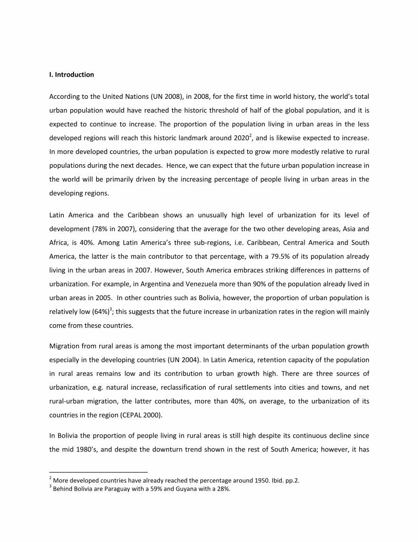
I. Introduction

According to the United Nations (UN 2008), in 2008, for the first time in world history, the world’s total

urban population would have reached the historic threshold of half of the global population, and it is

expected to continue to increase. The proportion of the population living in urban areas in the less

developed regions will reach this historic landmark around 20202, and is likewise expected to increase.

In more developed countries, the urban population is expected to grow more modestly relative to rural

populations during the next decades. Hence, we can expect that the future urban population increase in

the world will be primarily driven by the increasing percentage of people living in urban areas in the

developing regions.

Latin America and the Caribbean shows an unusually high level of urbanization for its level of

development (78% in 2007), considering that the average for the two other developing areas, Asia and

Africa, is 40%. Among Latin America’s three sub-regions, i.e. Caribbean, Central America and South

America, the latter is the main contributor to that percentage, with a 79.5% of its population already

living in the urban areas in 2007. However, South America embraces striking differences in patterns of

urbanization. For example, in Argentina and Venezuela more than 90% of the population already lived in

urban areas in 2005. In other countries such as Bolivia, however, the proportion of urban population is

relatively low (64%)3; this suggests that the future increase in urbanization rates in the region will mainly

come from these countries.

Migration from rural areas is among the most important determinants of the urban population growth

especially in the developing countries (UN 2004). In Latin America, retention capacity of the population

in rural areas remains low and its contribution to urban growth high. There are three sources of

urbanization, e.g. natural increase, reclassification of rural settlements into cities and towns, and net

rural-urban migration, the latter contributes, more than 40%, on average, to the urbanization of its

countries in the region (CEPAL 2000).

In Bolivia the proportion of people living in rural areas is still high despite its continuous decline since

the mid 1980’s, and despite the downturn trend shown in the rest of South America; however, it has

2 More developed countries have already reached the percentage around 1950. Ibid. pp.2.

3 Behind Bolivia are Paraguay with a 59% and Guyana with a 28%.

1

been projected that it will continue to fall during the following decades.4 Migration movements

originating in the rural area represent an annual 30% of the total migration flows in the country5, and

among those, rural-urban migrants represent an average of 59%,6 or approximately 26,700 households

per year. This number is expected to increase as already explained.

Todaro (1995) suggests several important questions in the study of migration that need to be addressed,

especially when the focus is on rural-urban migration. First, why do people migrate from their home

villages and what variables determine such decision? Second, how does migration affect the social and

economic development of the source and the destination regions? This paper concentrates on the first

of these questions.

It is widely accepted that economic considerations provide strong motivation to migrate.7 The absence

of crop insurance and shortage of liquidity are among the most important constraints that push rural

families to look for diversification across alternative sources of income, which will secure a source of

income not just for the migrants, but also for the family that stays behind in the village (Lucas 1997).

According to Taylor (1999), remittances represent the largest direct positive impact of migration on

incomes and production of the rural families, in particular, and on migrant sending areas in general.

Regmi and Tisdell (2002) explain that remittances are often the reason for the migration decision and its

most important consequence. The impact of remittances on migration varies across countries, and may

vary across regions within a country for several reasons. Impact depends on household characteristics;

the functioning of the market in which migration and remittances decisions are taken; constraints faced

by households; and, the tradition of migration/remittances-reception of the surrounding environment of

the households.

Despite the fact that remittances might not be the dominant source of income among rural households8,

their impact on income on those that receive them is considerable; based on case-studies in some

4 Since 1985 the decline in Bolivian rural population as a percentage of the total population has exceed the average

percentage of the rest of countries in South America by more than 1%, and it is projected to remain at that level for the next four decades (UN 2008). 5 The average includes migration flows in 1997 and 2002 from Tannuri-Pianto et. al. (2004). The other 70% is

originated in urban and metropolitan areas. 6 The remaining 41.4% are rural-rural migrants. Ibid. pp. 5.

7 Todaro (1995).

8 In Burkina Faso, only 6.3% of the rural households in the sample received internal remittances (Wourtese, 2008),

while in Guatemala the number was 14.6 % (Adams, 2004).

2

countries of the developing world, they represent up to 16% of the total household’s income9.

Unfortunately, no such information is available for Bolivia.

Among the large existing literature related to migration and remittances, two areas have been

extensively studied. The first relates to the effects of remittances on poverty and inequality; the

literature shows that remittances help reduce the incidence, depth and severity of poverty in developing

countries10; the evidence regarding the impact of remittances on inequality, however, has not been as

conclusive11. The second area relates to the motives of migrants for sending remittances; they range

from pure altruism (where the sole reason for the migrant for remitting is to support family

consumption back in the hometown), to pure self-interest (where remittances are made for the

aspiration to inherit or to invest in the rural town), or some combination of the two. Both areas have

been applied to migration across countries, and to migration within countries. However, in both cases

the analysis focused on the remitters’ characteristics and their contextual settings. 12

Adams et. al. (2008), using data from Ghana, takes a different approach. This paper analyzes

remittances in a framework where the focus was precisely on the origin of the income flows rather than

on the existence or not of migration assets in the rural household.

Finally, two are the main reasons that have been established to explain the presence of remittances

among the income sources. Taylor (1999) and Lucas (1997) suggest that remittances represent an

income diversification strategy. The World Bank (2006) posits that remittances ease working capital

constraints, and hence represent a source of liquidity for the farmer. This has yet to be tested

econometrically.

Therefore, the focus of the present work is on rural-urban migration, where migration remittances are

hypothesized to be an effort by rural households to overcome market failures for credit and insurance,

and hence a means to diversify their income sources into nonfarm activities. The rural households from

which the family members have been sent as migrants, their characteristics, and the contextual settings

9 In Burkina Faso, remittances as a share of total households income represent a 10.4% (Wourtese, 2008),

Guatemala on the same indicator is 15.78% (Adams, 2004), and Egypt 15% (Adams 1991). 10

See for example Adams et.al (2008) for Ghana, Wourtese (2008) for Burkina Faso, Taylor et. al (2005) for Mexico, and Adams (2004) for Guatemala. 11

The World Bank (2006) explains that the effect depends on who receives the remittances (the better-off or the less well-off), if we are considering the effects in the short or long term, and other variables that affect their distribution. 12

See for example Gopal and Tisdell (2002) for Nepal, Brown (1997) for the Pacific Island, Hoddinott (1992) for Kenya, and Lucas et. al. (1985) for Botswana.

3

in which they make decisions, is the framework we use to study the variables that make rural families

receive or not remittances, and diversify income into nonfarm activities or not.13

The analysis will be performed based on data from Bolivia and its rural-urban migrants. The existing

market failures that constrain production, the low urbanization rate of the country, and the prospects of

continuing and increasing migration from the countryside in the next decades, make the country an

attractive case to study. The distinct agroclimatic regions in which the country is geographically divided

will be properly considered when estimating the model to inquire regional differences.

The rest of the paper is organized as follows. In Section II the hypothesis regarding migration

remittances and their role for nonfarm income diversification strategies is proposed. Section III presents

the econometric model used to estimate the relationship between remittances and nonfarm income

diversification. Section IV outlines the database used for the modeling, and the variables involved in the

estimation process. Section IV presents the estimations’ results and relevant marginal probability

effects. Section V concludes.

II. The role of migration remittances in the farmers household’s budget

Remittances can affect households’ budget and wealth in different ways. Remittances directly increase

the income of the rural household that receives them; hence they could help poor farmers to escape

poverty. Remittances also contribute to smooth household consumption. They ease capital constraints,

faced primarily by poor rural farmers. Finally, remittances increase household expenditures (World

Bank, 2006). In this work, we focus our analysis in the role of migration remittances of providing working

capital.

Rural farmers choose between different types of income, which can be earned singly (no diversification)

or in various combinations (diversification). The alternative for rural residents are farm income, farm

income and remittances, farm income and income from other nonfarm activities, or finally from all three

sources of income simultaneously.

Before explaining the way in which we hypothesize how rural farmers decide on income diversification

through remittances, let us briefly make two notes in regards to migration decisions and the receipt of

remittances. First, not all migrants should be expected to migrate for reasons related to remittances.

13

Lucas (1997) establishes that one important group of factors that influence migration and remittances decisions are the contextual setting, or general characteristics of the sending community.

4

Even though an income diversification strategy through remittances may begin with the decision to send

family members away as migrants (e.g. rural-urban migration), the decision of sending migrants may be

motivated by other factors and necessities. Based on data provided by Andersen (2002) in his study on

rural-urban migration in Bolivia, at most 18% of the migrants had remittances as the primary reason

behind migration;14 but of course, not everyone migrant remits. Therefore, from the standpoint of

income diversification, the mere existence of remittances in the rural household is what matters, since

this is consistent with the desire to diversify income.

Second, following Niimi and Özden (2008), we assume that if remittances are observed as part of the

rural household’s income, it is because the household sent at least one family member away as migrant.

If it had not, no remittance would be observed. This rules out the possibility that the rural household

might receive remittances even if no family members have migrated; we treat this option as unlikely or

negligible.

We can now proceed with our proposition regarding the motivations and contextual conditionings

involved in the process of income diversification through migration remittances.

A good characterization of the limiting conditions that rural farmers in developing countries face is the

one developed by Lucas (1997), where the author states that agriculture is a high risk activity. Farmers

face the prospects of floods, droughts, pests and cattle disease for which insurance rarely exists, or

when it does exist, as Stark (1988) explains, the transaction costs may be prohibitive, especially for poor

small farmers. Hence, insurance may be impossible to obtain. If so, rural farmers must look for a

method of self-insurance, such as diversification across different sources of income. The object is to

develop sources of income that are not positively correlated with farm income, e.g. sending family

members as migrants to obtain remittances and/or diversify into other nonfarm activities.

Risks and lack of insurance are not, of course, the only limitation faced by rural farmers; lack of capital

and imperfect or inexistent credit markets might also constrain them (Taylor 1999) in their desire of

making farm and/or nonfarm investments (Taylor and Wyatt 1996).

14

Among rural-urban migrants, 50% stated that family reunion was the reason for migration, 26% said education, 4% due to job moved, and 2% for health; the remaining 18% mentioned job search as the reason for migrating to the urban area.

5

Under such characterization of the limitations faced by rural farmers, and the self-insurance strategies

that these agents follow to overcome them, a rural family may decide to diversify income15 using an

income source that counterbalances the lack of working capital due to the imperfect or inexistence

credit markets.16Therefore, we hypothesize that initially rural farmers diversify (e.g. through nonfarm

activities) as a self-insurance strategy against agricultural risks. However, if the farmer liquidity

constrained and faces an imperfect or inexistent credit market, he/she first need to loosen this

constraint in order to undertake any business venture off the farm. Therefore, remittances end up being

a means for income diversification, through the provision of working capital, to those households that

lack access to credit markets, or provide “cheaper” capital for those that can access the market but the

costs are extremely high.

In concordance with our hypothesis, we explore the effect of remittances on the propensity of rural

households to diversify income through nonfarm work, conditional on the characteristics of the

households and on the environment in which they make their decisions. The estimation method used

for this purpose is explained in the next section.

III. Econometric model and estimation

Given our hypothesis regarding the role of remittances in nonfarm income diversification strategies, the

goal is to model a situation in which the decision to remit affects the decision of a household to diversify

income through the nonfarm work. It is likely that unobserved factors affect both decisions for a typical

farmer and that the decisions share many of these.

The bivariate probit model, an extension of the probit model, allows the presence of two binary (0,1)

dependent variables correlated through their errors. Following Greene (2008), the outcomes of the two

discrete choices can be viewed as a result of an underlying regression or index function, which captures

the economic benefit calculation that leads to the decision of taking an action or not .

Denote each equation with subscript , and let be vectors of observed exogenous variables that affect

the utility of the decision-maker (e.g. household), be the error terms for the two possible discrete

outcomes, which are jointly normally distributed with means zero, variances equal to one, and, be the

15

Decisions on income diversification are now widely understood as a family strategy rather than a individualistic process, see for example Lucas (1997) and Taylor and Wyatt (1996). 16

The thesis that remittances are a diversification strategy has been widely analyzed and explained; see for example Taylor (1999) and Lucas (1997).

6

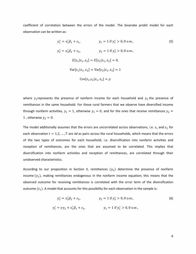
coefficient of correlation between the errors of the model. The bivariate probit model for each

observation can be written as:

(5)

where represents the presence of nonfarm income for each household and the presence of

remittances in the same household. For those rural farmers that we observe have diversified income

through nonfarm activities, , otherwise , and for the ones that receive remittances

, otherwise .

The model additionally assumes that the errors are uncorrelated across observations, i.e. and for

each observation are iid as pairs across the rural households, which means that the errors

of the two types of outcomes for each household, i.e. diversification into nonfarm activities and

reception of remittances, are the ones that are assumed to be correlated. This implies that

diversification into nonfarm activities and reception of remittances, are correlated through their

unobserved characteristics.

According to our proposition in Section II, remittances determine the presence of nonfarm

income , making remittances endogenous in the nonfarm income equation; this means that the

observed outcome for receiving remittances is correlated with the error term of the diversification

outcome . A model that accounts for this possibility for each observation in the sample is:

(6)

7

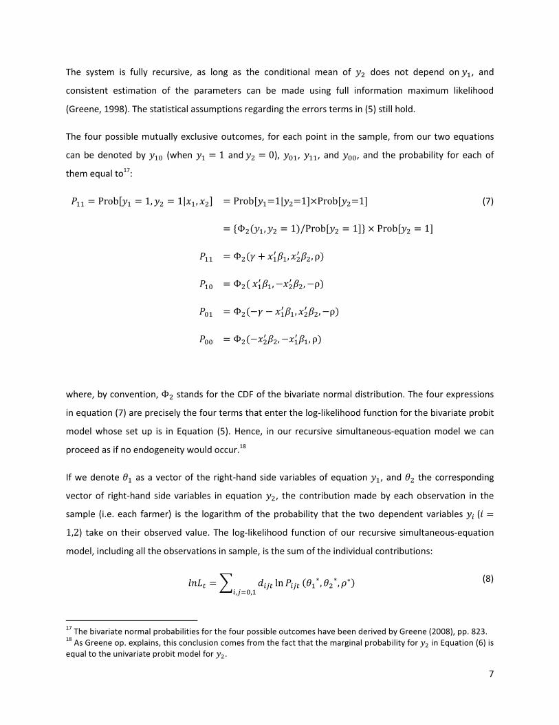
The system is fully recursive, as long as the conditional mean of does not depend on , and

consistent estimation of the parameters can be made using full information maximum likelihood

(Greene, 1998). The statistical assumptions regarding the errors terms in (5) still hold.

The four possible mutually exclusive outcomes, for each point in the sample, from our two equations

can be denoted by (when and ), , , and , and the probability for each of

them equal to17:

(7)

where, by convention, stands for the CDF of the bivariate normal distribution. The four expressions

in equation (7) are precisely the four terms that enter the log-likelihood function for the bivariate probit

model whose set up is in Equation (5). Hence, in our recursive simultaneous-equation model we can

proceed as if no endogeneity would occur.18

If we denote as a vector of the right-hand side variables of equation , and the corresponding

vector of right-hand side variables in equation , the contribution made by each observation in the

sample (i.e. each farmer) is the logarithm of the probability that the two dependent variables (

) take on their observed value. The log-likelihood function of our recursive simultaneous-equation

model, including all the observations in sample, is the sum of the individual contributions:

(8)

17

The bivariate normal probabilities for the four possible outcomes have been derived by Greene (2008), pp. 823. 18

As Greene op. explains, this conclusion comes from the fact that the marginal probability for in Equation (6) is equal to the univariate probit model for .

8

where is an indicator variable , equals one when its argument is true, and

zero otherwise, with and representing the actual choices of individual . In (6), equations and

describe a system of equations for which the parameters are to be estimated simultaneously. The

Full Information Maximum Likelihood (FIML) estimator is consistent and fully efficient for all the

parameters in the model (Greene, 1998).

Finally, we need to ensure the identification of the model. According to Maddala (1983), the

identification of the diversification equation requires that at least one variable from the remittances

equation be excluded from the diversification equation. Wilde (2000), however, establishes that in the

case of a bivariate model, the parameters are identified even if such exclusion restrictions do not exist.

He explains that identification is simply feasible based on the presence of varying exogenous regressors.

However, since identification based on exclusion restrictions is being found to be more robust (Yo ru k,

2009) we make sure to include those restrictions in the model.

IV. Data

The data used in the present work comes from the database of the Program for the Improvement of

Surveys and the Measurement of Living Conditions in Latin America and the Caribbean (MECOVI for its

acronym in Spanish)19, which is conducted by the INE (Bolivian Bureau of Census) in Bolivia, and provides

access to it through its web page www.ine.gov.bo.

The MECOVI’s have been conducted annually since 1999, and on-line information is available from the

surveys conducted during 1999 through 2002. Since each survey does not track the same households,

and some key questions are not asked in each survey, we perform a cross-section analysis for the survey

of the year 2000. The stratified sampling procedure in the MECOVI 2000 is designed to eliminate

sampling bias due to the household is included in the survey (Rivero and Mollinedo 2000).

The annual surveys collect data on such diverse topics such as income, expenditures, education, health,

employment, food consumption, assets holdings and migration. It needs to be emphasized, though, that

since the MECOVI surveys target variables related to the living conditions of the population and not

19

The Program is executed by the World Bank (IBRD), the Inter-American Development Bank (IDB) and the United Nations Economic Commission for Latin America and the Caribbean (ECLAC), as well as specialized institutions or agencies in countries participating in the Program. Subsequently other donors, such as Canada, Denmark, Germany, Japan, Norway, Sweden, UNDP, USA, and the Soros Foundation, have supported the Program.

9

migration and remittances specifically, they contain limited information on these topics. With respect to

migration, the information about migrants is available at the households of destination, and not at the

households of origin. This makes impossible to know if the migration assets are held by the rural

farmers, our target group.20 What we have is information regarding remittances, domestic and

international,21 and whether the households receive them or not. If they do, the exact amount is

provided. As Adams (2004) also establishes, it would be desirable to have information regarding the

migrants of the rural household. However, having detailed information about the characteristics and the

environment in which the farmers make decisions makes it possible to explore the role of remittances as

a diversification income strategy.

The MECOVI survey for 2000 covers sample units from urban and rural households; for the present work

we concentrate on the rural sample that comprises 2,108 households, or 9,092 persons, over 166

localities in the nine Departments of the country.22 However, among the total rural households only

1,960 are in our final sample since our goal is to estimate the degree of income diversification of the

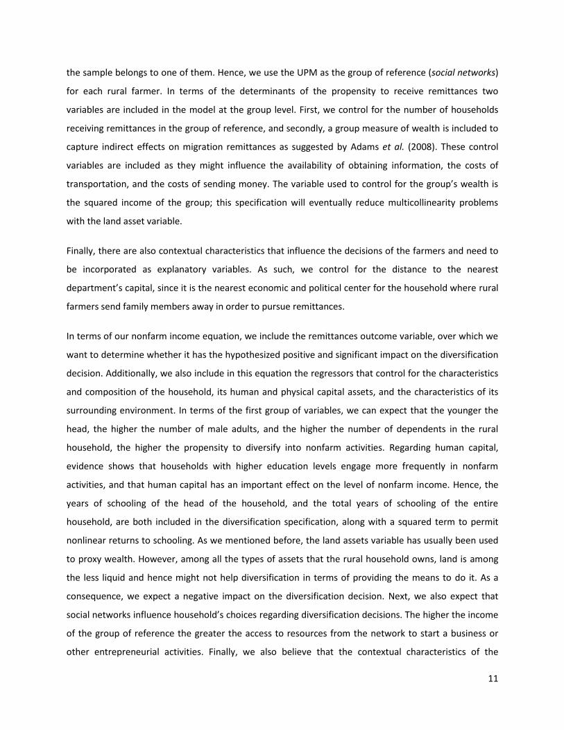
rural farmers thorough remittances and/or other nonfarm activities.23 Finally, the classification among

the 1,960 farmers according to income source is shown in Table 1.24

In the next sub-section, we specify the variables involved in the estimation of the bivariate probit model.

20

In relation to migration, the survey reports whether some member of a household is an immigrant, and if it is so, it provides information regarding the general location of the geographical area of origin (e.g. if the person has migrated from within the country they are asked the Department, Province and Municipality, and if they are from abroad, the country and city names). Unfortunately, this information is not enough to track the rural household from where the person would have migrated when the migration originated from another part of the country. The survey unfortunately does not ask if the households (rural or urban) have some members that have migrated and so are not present during the interview. Therefore, it is impossible to include information regarding the migrants that rural households might have sent, and then among those, to differentiate the ones that receive remittances. 21

The term domestic applies to remittances that are sent from anywhere within the country, and international for those remittances that are sent from abroad. 22

From the total 2,108 households, 825 are located in the Altiplano region, 756 in the Valles and, 527 in the Llanos. The survey also classifies the households according to their location into two groups: rural populated centers (212 households) and rural dispersed areas (1,896 households). 23

Rural households, whose primary and/or secondary occupation is not related with farm work, have been dropped from the sample. 24

We later drop 257 observations, and end up estimating the model with 1,703 households that have complete information.

Table 1. Rural households classification according to income source

Only farmers 1,086

Farmers receiving remittances 219

Farmers with nonfarm income 559

Farmers receiving both, remittances and

income from nonfarm work96

10

4.1 The independent variables

The variables included as explanatory are individual-specific and can broadly be classified within four

groups. These include household characteristics (such as the age of the head and the number of adult

and children members), household human capital assets (proxied by the head’s education attainment

and total number of years of education in the household), physical assets of the household (proxied by

its landholdings), and the contextual characteristics of the surrounding environment where the rural

household resides (proxied by some characteristics of the social networks of the household, and

distance to the nearest capital of Department).

The logic behind those explanatory variables lies, in general, on the standard available literature on

migration/remittances (Adams et. al. 2008) and diversification into nonfarm activities. In the case of the

characteristics of the household, we can expect that if the altruistic motive is behind remittances (Lucas

and Stark, 1985), households with older heads, fewer male members, and more children are more likely

to receive remittances. Migrants can be thought to remit more if among those left behind are elderly,

with little labor force, and many dependents25. With respect to human capital assets, and following

Hoddinot (1992), we can expect that the higher the education attainment the better access to the

formal sector of the rural labor market, and hence the rural household is less likely to be liquidity

constrained. Hence we expect a negative impact on the remittances outcome. We proxy human capital

with two variables: the years of schooling of the head of the household, and the total years of schooling

of the entire household. A squared specification is included to permit nonlinear returns to schooling.

Asset holdings, which are proxied by landholdings, have been extensively used to approximate the

wealth of the household in the study of migration/remittances (Wourtese 2008). If the aspiration to

inherit, for example, is an important reason to remit, as hypothesized (Lucas and Stark, 1985), the larger

the potential of inheritance, the higher the probability of the rural household to receive remittances. As

a consequence, we use landholdings per capita in the remittances equation to capture this effect.

It has also been widely explained and empirically demonstrated that social networks greatly affect the

decisions made by entities such a household (see for example Taylor et. al. 2005). For sampling reasons,

the INE divides the country geographically into UPM’s (Primary Sample Units)26, and each observation in

25

The composition of the household variables considers all the members left behind, after some have migrated. 26

The INE divides Bolivia into approximately 21,000 UPM, each bringing together an average of 50 housings. The master sample used for the survey in 2000 contains 2,500 UPM, and the final sample for the MECOVI 2000 encompasses 150 UPM. More details in http://www.eclac.cl/deype/mecovi/taller9.htm.

11

the sample belongs to one of them. Hence, we use the UPM as the group of reference (social networks)

for each rural farmer. In terms of the determinants of the propensity to receive remittances two

variables are included in the model at the group level. First, we control for the number of households

receiving remittances in the group of reference, and secondly, a group measure of wealth is included to

capture indirect effects on migration remittances as suggested by Adams et al. (2008). These control

variables are included as they might influence the availability of obtaining information, the costs of

transportation, and the costs of sending money. The variable used to control for the group’s wealth is

the squared income of the group; this specification will eventually reduce multicollinearity problems

with the land asset variable.

Finally, there are also contextual characteristics that influence the decisions of the farmers and need to

be incorporated as explanatory variables. As such, we control for the distance to the nearest

department’s capital, since it is the nearest economic and political center for the household where rural

farmers send family members away in order to pursue remittances.

In terms of our nonfarm income equation, we include the remittances outcome variable, over which we

want to determine whether it has the hypothesized positive and significant impact on the diversification

decision. Additionally, we also include in this equation the regressors that control for the characteristics

and composition of the household, its human and physical capital assets, and the characteristics of its

surrounding environment. In terms of the first group of variables, we can expect that the younger the

head, the higher the number of male adults, and the higher the number of dependents in the rural

household, the higher the propensity to diversify into nonfarm activities. Regarding human capital,

evidence shows that households with higher education levels engage more frequently in nonfarm

activities, and that human capital has an important effect on the level of nonfarm income. Hence, the

years of schooling of the head of the household, and the total years of schooling of the entire

household, are both included in the diversification specification, along with a squared term to permit

nonlinear returns to schooling. As we mentioned before, the land assets variable has usually been used

to proxy wealth. However, among all the types of assets that the rural household owns, land is among

the less liquid and hence might not help diversification in terms of providing the means to do it. As a

consequence, we expect a negative impact on the diversification decision. Next, we also expect that

social networks influence household’s choices regarding diversification decisions. The higher the income

of the group of reference the greater the access to resources from the network to start a business or

other entrepreneurial activities. Finally, we also believe that the contextual characteristics of the

12

environment where the rural household resides influence the decisions of the farmers regarding

undertaking nonfarm activities. The distance to the nearest department’s capital is included here as

well, since the department capital is the nearest economic and political center for the rural household,

where they might find nonfarm work.

Finally, dummy variables are conveniently included to capture the existence of possible regional effects.

Two of them are used to discriminate among the three agroclimatic regions (i.e. Altiplano, Valles, and

Llanos), and a third one to differentiate the regions where coca leaf production exits.

V. Estimation results

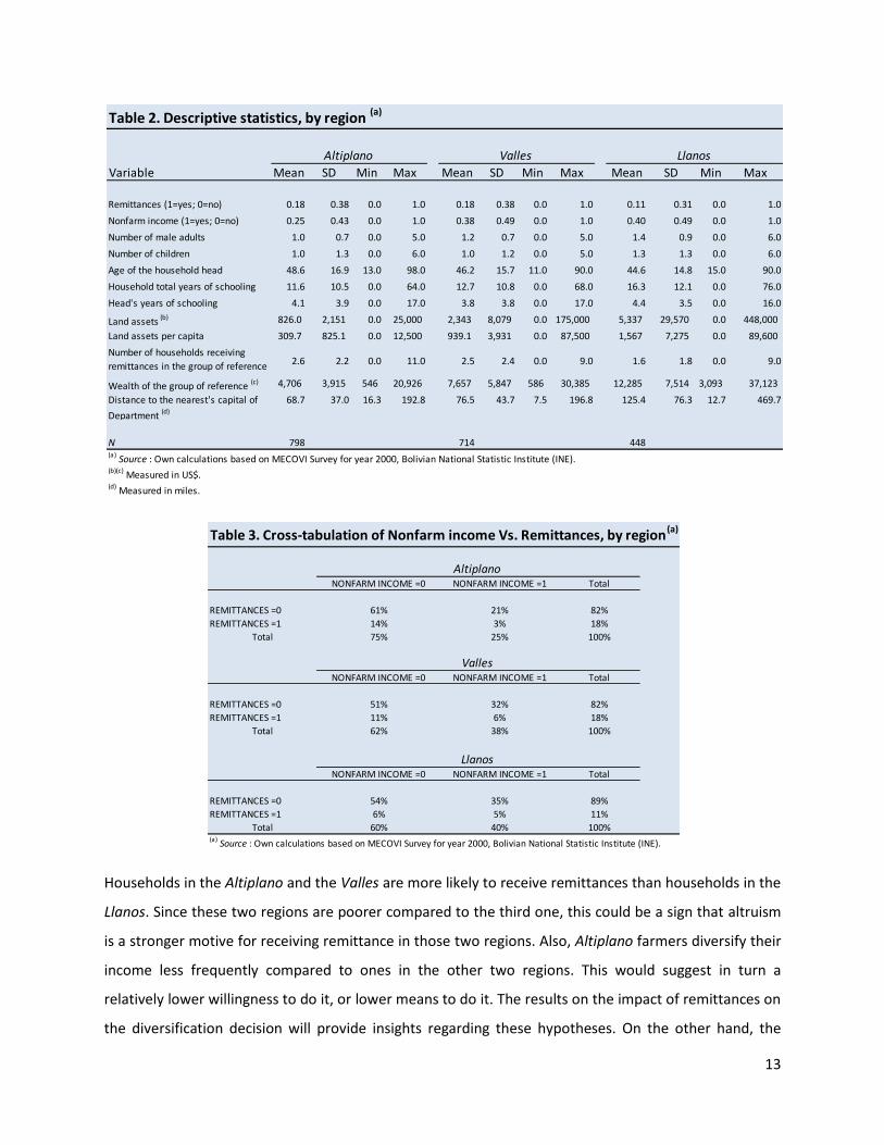
Table 2 includes some descriptive statistics of the variables used in the nonfarm income and remittances

equations of our bivariate probit model. Recall that nonfarm income refers to whether a household

diversifies farm income from nonfarm activities, and remittances in turn, to whether the household

receives remittances. Since we want to contrast among households coming from the three different

geographic regions, we present the data in this and the following tables, in regional terms.

With respect to human capital, Table 2 shows that households in the Llanos have more human capital

than households living in the other two regions. It also shows that while households living in the Llanos

have the highest mean land value, the asset is highly dispersed in all three regions. In terms of skewness

the asset is positively skewed, with the Valles region having a relative longer tail.27

In terms of our two binary outcomes, Table 3 provides a cross-tabulation statistics for each region.

According to it, a smaller percentage of households in the Llanos receive remittances compared to the

other two regions; however, it is precisely in that region where there is a higher portion of the

households having income coming from nonfarm work, while the smallest percentage of households

with nonfarm income among regions is in the Altiplano.

27

The overall skewness value for land is 20.11. In regional terms, the measure is 7.27 for the Altiplano, 16.29 for the Valles, and 11.13 for the Llanos.

13

Households in the Altiplano and the Valles are more likely to receive remittances than households in the

Llanos. Since these two regions are poorer compared to the third one, this could be a sign that altruism

is a stronger motive for receiving remittance in those two regions. Also, Altiplano farmers diversify their

income less frequently compared to ones in the other two regions. This would suggest in turn a

relatively lower willingness to do it, or lower means to do it. The results on the impact of remittances on

the diversification decision will provide insights regarding these hypotheses. On the other hand, the

Table 2. Descriptive statistics, by region (a)

Variable Mean SD Min Max Mean SD Min Max Mean SD Min Max

Remittances (1=yes; 0=no) 0.18 0.38 0.0 1.0 0.18 0.38 0.0 1.0 0.11 0.31 0.0 1.0

Nonfarm income (1=yes; 0=no) 0.25 0.43 0.0 1.0 0.38 0.49 0.0 1.0 0.40 0.49 0.0 1.0

Number of male adults 1.0 0.7 0.0 5.0 1.2 0.7 0.0 5.0 1.4 0.9 0.0 6.0

Number of children 1.0 1.3 0.0 6.0 1.0 1.2 0.0 5.0 1.3 1.3 0.0 6.0

Age of the household head 48.6 16.9 13.0 98.0 46.2 15.7 11.0 90.0 44.6 14.8 15.0 90.0

Household total years of schooling 11.6 10.5 0.0 64.0 12.7 10.8 0.0 68.0 16.3 12.1 0.0 76.0

Head's years of schooling 4.1 3.9 0.0 17.0 3.8 3.8 0.0 17.0 4.4 3.5 0.0 16.0

Land assets (b) 826.0 2,151 0.0 25,000 2,343 8,079 0.0 175,000 5,337 29,570 0.0 448,000

Land assets per capita 309.7 825.1 0.0 12,500 939.1 3,931 0.0 87,500 1,567 7,275 0.0 89,600

Number of households receiving

remittances in the group of reference 2.6 2.2 0.0 11.0 2.5 2.4 0.0 9.0 1.6 1.8 0.0 9.0

Wealth of the group of reference (c) 4,706 3,915 546 20,926 7,657 5,847 586 30,385 12,285 7,514 3,093 37,123

Distance to the nearest's capital of

Department (d)

68.7 37.0 16.3 192.8 76.5 43.7 7.5 196.8 125.4 76.3 12.7 469.7

N 798 714 448(a)

Source : Own calculations based on MECOVI Survey for year 2000, Bolivian National Statistic Institute (INE).(b)(c)

Measured in US$.(d) Measured in miles.

Altiplano Valles Llanos

Table 3. Cross-tabulation of Nonfarm income Vs. Remittances, by region(a)

NONFARM INCOME =0 NONFARM INCOME =1 Total

REMITTANCES =0 61% 21% 82%

REMITTANCES =1 14% 3% 18%

Total 75% 25% 100%

NONFARM INCOME =0 NONFARM INCOME =1 Total

REMITTANCES =0 51% 32% 82%

REMITTANCES =1 11% 6% 18%

Total 62% 38% 100%

NONFARM INCOME =0 NONFARM INCOME =1 Total

REMITTANCES =0 54% 35% 89%

REMITTANCES =1 6% 5% 11%

Total 60% 40% 100%(a)

Source : Own calculations based on MECOVI Survey for year 2000, Bolivian National Statistic Institute (INE).

Altiplano

Valles

Llanos

14

statistics also show that income diversification is more widespread in the Llanos. This could be driven by

a stronger willingness to undertake risk-spreading strategies in the region, and that households in that

region have more successfully found ways to reduce liquidity constraints. The Valles region is more of a

mixed story, with higher number of households receiving remittances, but a relatively high proportion of

them involve in nonfarm employment. Here we also want to investigate and bring some insights

regarding the role of remittances in the diversification strategies, in these high prone nonfarm

employment regions.

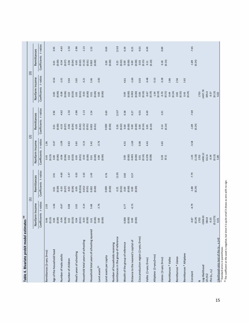
The full information maximum likelihood estimates from the bivariate probit model are given in Table 4.

As mentioned already, the estimator is consistent and fully efficient for all the parameters in the model.

Each set of results, marked with a number at the top, show the estimates of the remittances outcome

equation in the second column, and the estimates for the presence of nonfarm income in the first

column. Column (1) includes, in the nonfarm income equation, the remittances discrete variable, all the

household characteristics and human capital variables, along with a social network variable (wealth of

the group of reference), and a contextual variable (distance to the nearest capital of Department). The

specification of land in the diversification equation is the total value of the asset, and it acts as the

exclusion restriction that helps identify the presence of the remittances equation. The remittances

equation on the other hand, also includes the same household characteristics and human capital

variables, as well as the same social network and contextual variables. Additionally, we also add the

household’s land assets per capita, and the number of households receiving remittances in the group of

reference. These two variables are the exclusion restrictions that identify the nonfarm income equation.

15

Tab

le 4

. B

ivar

iate

pro

bit

mo

de

l est

imat

es

(a)

Co

effi

cien

tst

-rat

ios

Co

effi

cien

tst

-rat

ios

Co

effi

cien

tst

-rat

ios

Co

effi

cien

tst

-rat

ios

Co

effi

cien

tst

-rat

ios

Co

effi

cien

tst

-rat

ios

Rem

itta

nce

s (1

=yes

; 0=n

o)

0.4

62

.03

0.4

51

.96

(0.2

3)

(0.2

3)

Age

of

the

ho

use

ho

ld h

ead

0.0

0-1

.06

0.0

13

.91

0.0

0-0

.47

0.0

13

.96

0.0

0-0

.54

0.0

13

.95

(0.0

0)

(0.0

0)

(0.0

0)

(0.0

0)

(0.0

0)

(0.0

0)

Nu

mb

er o

f m

ale

adu

lts

-0.0

4-0

.67

-0.3

3-4

.60

-0.0

6-1

.09

-0.3

3-4

.62

-0.0

6-1

.01

-0.3

4-4

.63

(0.0

6)

(0.0

7)

(0.0

6)

(0.0

7)

(0.0

6)

(0.0

7)

Nu

mb

er o

f ch

ildre

n0

.02

0.6

8-0

.02

-1.4

70

.02

0.6

3-0

.06

-1.5

00

.02

0.6

4-0

.06

-1.5

0

(0.0

3)

(0.0

4)

(0.0

3)

(0.0

4)

(0.0

3)

(0.0

4)

He

ad's

yea

rs o

f sc

ho

olin

g0

.04

3.0

3-0

.05

-3.0

20

.05

3.6

5-0

.05

-2.8

60

.05

3.6

5-0

.05

-2.8

6

(0.0

1)

(0.0

16

)(0

.01

)(0

.02

)(0

.01

)(0

.02

)

Ho

use

ho

ld t

ota

l yea

rs o

f sc

ho

olin

g-0

.03

-3.1

4-0

.01

2-1

.02

-0.0

3-3

.15

-0.1

32

-1.1

3-0

.03

-3.2

1-0

.13

2-1

.13

(0.0

0)

(0.0

1)

(0.0

0)

(0.0

1)

(0.0

0)

(0.0

1)

Ho

use

ho

ld t

ota

l yea

rs o

f sc

ho

olin

g sq

uar

ed0

.01

5.4

80

.00

21

.49

0.0

15

.42

0.0

02

1.5

40

.01

5.4

60

.00

21

.53

(0.0

0)

(0.0

0)

(0.0

0)

(0.0

1)

(0.0

0)

(0.0

0)

Lan

d a

sset

s(b)

0.0

0-2

.76

0.0

0-2

.76

0.0

0-2

.82

(0.0

0)

(0.0

0)

(0.0

0)

Lan

d a

sset

s p

er c

apit

a0

.00

00

.76

0.0

00

0.6

90

.00

0.6

9

(0.0

0)

(0.0

0)

(0.0

0)

Nu

mb

er o

f h

ou

seh

old

s re

ceiv

ing

rem

itta

nce

s in

th

e gr

ou

p o

f re

fere

nce

0.2

51

2.9

50

.26

12

.67

0.2

51

2.6

3

(0.0

2)

(0.0

2)

(0.0

2)

Wea

lth

of

the

gro

up

of

refe

ren

ce0

.00

06

.77

0.0

00

.82

0.0

04

.55

0.0

00

.38

0.0

04

.61

0.0

00

.39

(0.0

0)

(0.0

0)

(0.0

0)

(0.0

0)

(0.0

0)

(0.0

0)

Dis

tan

ce t

o t

he

nea

rest

's c

apit

al o

f 0

.00

-0.7

30

.00

0.5

7-0

.00

1-1

.69

0.0

00

.27

-0.0

01

-1.6

00

.00

0.2

5

(0.0

0)

(0.0

0)

(0.0

0)

(0.0

0)

(0.0

0)

(0.0

0)

Co

ca p

rod

uct

ion

reg

ion

(1

=yes

; 0=n

o)

0.0

10

.08

0.0

0-0

.01

0.0

00

.03

-0.0

3-0

.01

(0.1

0)

(0.1

4)

(0.1

0)

(0.1

5)

Va

lles

(1

=yes

; 0=n

o)

0.3

78

4.4

30

.05

0.4

9-0

.67

-3.4

80

.11

0.4

9

(0.0

8)

(0.1

0)

(0.1

9)

(0.1

0)

Alt

ipla

no

(1

=yes

;0=n

o)

-1.0

4-5

.53

(0.1

9)

Lla

no

s (

1=y

es; 0

=no

)0

.39

3.6

50

.14

1.0

1-0

.70

-3.2

80

.18

0.8

9

(0.1

)(0

.14

)(0

.21

)(0

.14

)

Rem

itta

nce

s *

Va

lles

0.4

41

.86

(0.2

4)

Rem

itta

nce

s *

Lla

no

s0

.82

2.5

6

(0.3

2)

Rem

itta

nce

s *

Alt

ipla

no

0.4

31

.62

(0.2

4)

Co

nst

ant

-0.8

7-4

.79

-1.8

8-7

.79

-1.0

5-5

.58

-1.8

9-7

.69

-1.8

9-7

.65

(0.2

4)

(0.2

4)

(1.1

8)

(0.2

4)

(0.2

4)

N1

70

31

70

31

70

3

Log-

likel

iho

od

-15

04

.03

-14

90

.12

-14

97

.78

LR c

hi2

58

4.8

61

2.6

69

5.0

rho (ε 1

, ε2)

-0.3

3-0

.34

-0.3

7

(0.1

27

3)

(0.1

3)

(0.1

3)

Like

lihood-rat

io tes

t of rh

o (ε 1

, ε2)=

06

.01

5.8

06

.82

(a) S

tan

dar

d e

rro

rs in

par

enth

eses

.(b

) Th

e co

effi

cien

t o

n t

he

asse

t is

neg

ativ

e, b

ut

sin

ce it

is q

uit

e sm

all i

t sh

ow

s as

zer

o w

ith

no

sig

n.

(1)

(2)

(3)

No

nfa

rm In

com

eR

emit

tan

ces

No

nfa

rm In

com

eR

emit

tan

ces

No

nfa

rm In

com

eR

emit

tan

ces

16

As we can see from this first set of results, remittances are highly and positively related to

diversification. The head’s level of schooling, household total years of schooling, and income of the

reference group each have positive and significant impacts on the probability of income diversification.

The results on the total years of education for the household are quite interesting. Given the signs of the

coefficients, there exists a minimum education level (i.e. 1.5 years) above which the impact of education

on the probability to diversify income is not only positive, but increasingly positive. Below such

threshold, the impact is negative which can be interpreted as for those extremely low education levels,

the returns to education from farm work and from nonfarm work are similar. The coefficient of the land

assets variable is significant and with the expected sign, but since its magnitude is quite small, the

impact of the variable is almost negligible.

In turn, the remittances decision is, as expected, positively affected by the age of the household’s head

and adversely impacted by the number of male adults. In terms of human capital, the head’s number of

years of education reduces the probability of receiving remittances. The more educated the head of the

household, the less likely to receive remittances due to a loosening liquidity constrain. The number of

dependents, the income of the reference group, the value of land assets per capita, and distance to the

nearest capital of Department, have no effect on the propensity of remittances. Finally, the results show

that migration networks are an important consideration for remittances. The higher the number of

households in the social network who receive remittances, the higher the probability for each of them

to receive remittances as well.

In terms of the correlation coefficient between the two structural disturbances, rho, it has an estimated

value of -0.33. Given the standard error for the parameter (0.13), the Wald statistic for the hypothesis

that is 6.06 which is greater than the critical value for . This result suggests the likely

existence of unobservable characteristics of the households that influence both outcomes. An

asymptotic similar test to the Wald statistic was also obtained automatically after the estimation of the

model of Column (1).The value of a likelihood-ratio test of again confirms our earlier

results. With a test statistic of 5.54, the null hypothesis is rejected at the 5% level of significance.28

Therefore, the simultaneous estimation of both equations appears to be justified relative to the

estimation of independent probit models. The bivariate probit is thus consistent and provides fully

efficient estimates for our model (Greene 1998). The negative sign of the correlation coefficient implies

28

An extensive analysis of the different methods available to test the hypothesis , in simultaneous equations models, and involving limited dependent variables, can be found in Monfardini et. al. (2008).

17

that unobserved and/or unmeasured factors that increase the probability of receiving remittances also

decrease the nonfarm income diversification propensity. Finally, as Greene and Seaks (1998) show, the

results of the likelihood-ratio test can also be used, asymptotically, as a Hausman test for the exogeneity

of the remittances discrete outcome in the diversification equation. This means that the correlation

results also suggest that receiving remittances is, as expected, an endogenous variable in the model. Its

positive and highly significant coefficient confirms the role of remittances in relaxing capital constraints

that frequently prevent rural farmers from diversifying its sources of income.

The positive and significant effect of remittances on the nonfarm income diversification equation

remains robust to different specifications of the model as it is shown in Table 3. Column (2) adds two

dummy variables to the model to explore the possible existence of intercept regional differences. The

first one includes three categories to distinguish among the three geographic regions, and the other

aims to differentiate the regions where coca leaves are produced. The regional dummies for the Valles

and Llanos regions are found to be significant for the nonfarm income equation, (although not for

remittances), but the one for the coca leaves production region is not significant for neither of the

equations. 29

Independently of the individual significance of the dummy regional variables, we also need to test

whether they altogether significantly improve the prediction of our outcomes. This was done using the

likelihood-ratio test of the null hypothesis all regional dummy coe cients e ual to ero. Since the

test statistic value of 27.84 ( -value 0.000) was significantly larger compared to the relevant critical

value, there was sufficient evidence of the joint significance of the regional dummy variable.30

Based on those results and on the rejection of the equality of the model parameters across regions for

the income diversification equation, but not for the remittances equation,31 the last set of results in

Table 4, Column (3), includes interaction terms for the three regional dummy variables with the

remittances discrete outcome in the nonfarm income equation. This last specification aims to provide

29

The Valles and Llanos regional dummies coefficients represent deviations with respect to the reference category Altiplano, which has been dropped as customary to avoid multicollinearity. 30

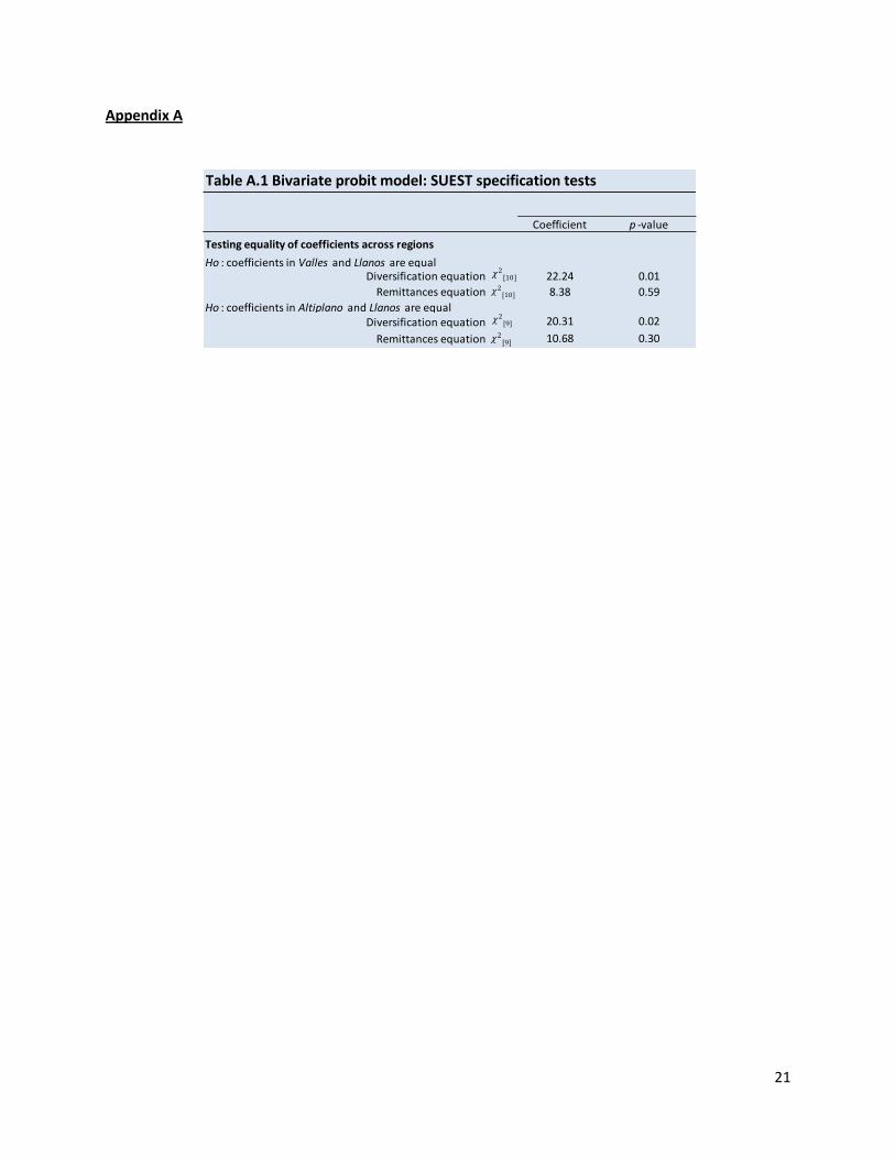
We also run the test including a dummy variable for coca leaf production regions (1 if the household is located in a region where it has been established there is coca production and 0 otherwise); the results confirmed the appropriateness of the inclusion of such regional dummy variables in the model. 31 We formally tested if the estimated coefficients for the three agroclimatic regions were equal to each other in

terms of each of the two equations in the model. We used the SUEST test, a variation of the Hausman specification test that ensures that the test will be well defined (i.e. the estimator of the variance of the difference between the two estimators is guaranteed to be positive semidefinite). The test statistic has a Chi-square distribution with degrees of freedom (White, 1982). The detailed results for the SUEST test are found in Appendix A.

18

more insights regarding the existence of regional effects in terms of the impact of remittances on the

nonfarm income diversification decision. The resulting coefficients show that two out of three regional

interaction coefficients are positive and significant at conventional levels. The coefficient for the

Altiplano region is positive and nearly significant at 10%. In terms of magnitudes, remittances in the

Llanos have a larger effect on diversification than they do in the Valles region.

Our battery of specification tests includes two final steps. First, we need to make sure that our

interaction terms for the three regions are jointly significant, and hence improve the specification of the

model. The Hausman test of the constraint that those coefficients are all zero has a chi-squared

distribution with 3 degrees of freedom. The resulting statistic of 6.75 with a -value of 0.07 allow us to

reject the null hypothesis at the 10% level. Secondly, we want to know if our regional interaction terms’

coefficients are all statistically equal to each other. Again for this purpose we use a Hausman test which

in this case has a chi-squared distribution with 2 degrees of freedom. The test statistic of 2.47 with a -

value of 0.292, tells us that there is no enough evidence to reject the null hypothesis of equality. This of

course could have been anticipated based on the almost identical coefficients of the Altiplano and Valles

regions.

It is worth to note that among all the different specifications in Table 4, the control variables have

always maintained their sign and significance level.

Before examining the magnitudes of the marginal effects, one more check of the specification is

performed. A consistent estimation of the parameters depends on the exogeneity of diversification in

the remittances equation. If it is endogenous then the system is not fully recursive and the estimates will

not be meaningful. Although this proposition is not directly testable, the possibility that the causality

should be reversed can be explored. To that effect the model is estimated treating the diversification as

being determined by all of its factors, save remittances, and treating diversification as an endogenous

determinant of remittances. This basically flips the model around; if diversification is insignificant in the

remittances equation then we have indirect evidence that the two are not jointly determined.

Thus, another bivariate probit model is estimated, but this time with the nonfarm income variable as

endogenous variable in the remittances equation. The estimated coefficient is -0.36 with a standard

error of 1.03. These results are consistent with the original specification that remittances affect

diversification and not vice versa.

19

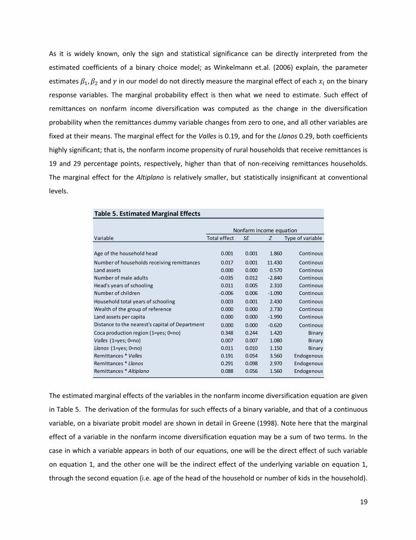
As it is widely known, only the sign and statistical significance can be directly interpreted from the

estimated coefficients of a binary choice model; as Winkelmann et.al. (2006) explain, the parameter

estimates and in our model do not directly measure the marginal effect of each on the binary

response variables. The marginal probability effect is then what we need to estimate. Such effect of

remittances on nonfarm income diversification was computed as the change in the diversification

probability when the remittances dummy variable changes from zero to one, and all other variables are

fixed at their means. The marginal effect for the Valles is 0.19, and for the Llanos 0.29, both coefficients

highly significant; that is, the nonfarm income propensity of rural households that receive remittances is

19 and 29 percentage points, respectively, higher than that of non-receiving remittances households.

The marginal effect for the Altiplano is relatively smaller, but statistically insignificant at conventional

levels.

The estimated marginal effects of the variables in the nonfarm income diversification equation are given

in Table 5. The derivation of the formulas for such effects of a binary variable, and that of a continuous

variable, on a bivariate probit model are shown in detail in Greene (1998). Note here that the marginal

effect of a variable in the nonfarm income diversification equation may be a sum of two terms. In the

case in which a variable appears in both of our equations, one will be the direct effect of such variable

on equation 1, and the other one will be the indirect effect of the underlying variable on equation 1,

through the second equation (i.e. age of the head of the household or number of kids in the household).

Table 5. Estimated Marginal Effects

Variable Total effect SE Z Type of variable

Age of the household head 0.001 0.001 1.860 Continous

Number of households receiving remittances 0.017 0.001 11.430 Continous

Land assets 0.000 0.000 0.570 Continous

Number of male adults -0.035 0.012 -2.840 Continous

Head's years of schooling 0.011 0.005 2.310 Continous

Number of children -0.006 0.006 -1.090 Continous

Household total years of schooling 0.003 0.001 2.430 Continous

Wealth of the group of reference 0.000 0.000 2.730 Continous

Land assets per capita 0.000 0.000 -1.990 Continous

Distance to the nearest's capital of Department 0.000 0.000 -0.620 Continous

Coca production region (1=yes; 0=no) 0.348 0.244 1.420 Binary

Valles (1=yes; 0=no) 0.007 0.007 1.080 Binary

Llanos (1=yes; 0=no) 0.011 0.010 1.150 Binary

Remittances * Valles 0.191 0.054 3.560 Endogenous

Remittances * Llanos 0.291 0.098 2.970 Endogenous

Remittances * Altiplano 0.088 0.056 1.560 Endogenous

Nonfarm income equation

20

A second case occurs when a variable appears just in the nonfarm income diversification equation, in

which case the effect of the explanatory variable is direct (i.e. the endogenous variable remittances

interacting with the regions, and land assets). We yet have a third possibility for other variables, such as

land assets per capita, that only appears in the remittances equation, and which marginal effect on

nonfarm income diversification decision will be indirect.

VI. Conclusions

This paper uses a nationally-representative household survey to study the role of migration remittances

in nonfarm income diversification strategies in Bolivia. There are three main findings.

First, and according to the literature, migration remittances represent a complementary income source

for rural households since they provide them with liquidity. The calculation of the marginal probability

effects show that, at the national level, nonfarm income propensity of rural households that receive

remittances is 13 percentage points higher than that of non-receiving remittances households.

Second, the results also suggest that the variable remittances is, in fact, endogenous and with a

significant effect on nonfarm income diversification; not taking this effect into account could result in

biased and inconsistent estimates. The significance of the correlation coefficient justifies the use of the

biprobit estimation model.

Third, accounting for the existence of significant regional differences, the paper finds that remittances

has a substantial positive effect on nonfarm income diversification in the Valles (with a marginal effect

of 0.19) and Llanos (with a marginal effect of 0.29) regions, but not in the Altiplano. These results are

consistent with the profile outlined for the existence of two different types of rural farmers in the

country. The small poor farmers, mainly located in the Andean region, are viewed as practicing

subsistent farming, where the reception of remittances may have the sole objective of supporting

consumption. In the other two regions, however, the existence of capitalist farming, oriented to the

domestic as well as foreign markets, could help explain the stronger willingness among those farmers to

undertake risk-spreading strategies. The imperfect and sometimes inexistent insurance and credit

markets make them search for diversified income sources off the farm. Hence, remittances are used in

those two regions as a source of liquidity that could help compensate the imperfect functioning of the

capital and credit markets in the country.

21

Appendix A

Table A.1 Bivariate probit model: SUEST specification tests

Testing equality of coefficients across regions

Ho : coefficients in Valles and Llanos are equalDiversification equation

Remittances equation

Ho : coefficients in Altiplano and Llanos are equalDiversification equation

Remittances equation

8.38 0.59

20.31 0.02

10.68 0.30

Coefficient p -value

22.24 0.01 2[10]

2[10]

2[9]

2[9]

22

References

Adams, Jr. R., A. Cuecuecha, and J. Page (2008). Impact of remittances on poverty and inequality in Ghana. World Bank Policy Research Working Paper 4732, Washington D.C.

Adams, Jr. R. (2004). Remittances and poverty in Guatemala. World Bank Policy Research Working Paper 3418, Washington D.C.

Adams, Jr. R. (1991). The Effects of International Remittances on Poverty, Inequality and Development in Rural Egypt. Research Report 86. International Food Policy Research Institute, Washington, DC. Andersen, L. (2002). Rural-urban migration in Bolivia: Advantages and disadvantages. Institute for Socio-Economic Research. La Paz Bolivia. (Manuscript).

Brown, R. (1997). Estimating remittance functions for Pacific Island migrants. World Development, Vol. 25(4): 613-626.

Comision Economica para America Latina y el Caribe (CEPAL) 2000. De la urbanizacion acelerada a la consolidación de los asentamientos humanos en America Latina y el Caribe: El espacio regional. Santiago de Chile: Centro de las Naciones Unidas para los Asentamientos Humanos (Habitat).

Gopal, R. and C. Tisdell (2002). Remitting Behavior of Nepalese Rural-to-Urban Migrants: Implications for Theory and Policy, Journal of Development Studies, Vol. 38 (3): 76-94. Greene, L. and T. Seaks (1998). A hausman test for a dummy variable in probit. Applied Economics Letters, Vol. 5: 321-323.

Greene, W. (2008). Econometric Analysis, sixth ed. Upper Saddle River, N.J.: Pearson/Prentice Hall.

Greene, W. (1998). Gender Economics Courses in liberal Arts Colleges: Further Results. Journal of Economic Education, Vol. 29 (4): 291-300.

Hoddinot, J. (1992). Modelling remittance flow in Kenya. Journal of African Studies, Vol. 1(2):206-232. Lucas, R. (1997). Internal Migration in Developing Countries, Handbook of Population and Family Economics, edited by M.R. Rosenzweig and O. Stark. London: Elsevier Science B.V.

Lucas, R. (1985).Motivation to remit: Evidence from Botswana. Journal of Political Economy, Vol. 93 (5): 901-918.

Maddala, G. (1983). Limited-Dependent and Qualitative Variables in Econometrics, Cambridge: Cambridge University Press. Monfardini, C. and R. Radice (2008). Testing Exogeneity in the Bivariate Probit Model: A Monte Carlo Study. Oxford Bulletin of Economics and Statistics, Vol. 70(2), pages 271-282, 04. Niimi, Y. and Ç. Özden (2008). Migration and Remittances in Latin America: Patterns and determinants, in Remittances and Development: Lessons from Latin America, edited by P. Fajnzylber and J. H. Lopez. Washington DC: The World Bank. Rivero, F. and F. Mollinedo (2002). Diseno y construccion de los marcos de muestreo para las encuestas de hogares; documento presentado en el Taller #9 del Programa para el Mejoramiento de las Encuestas y la Medicion de las Condiciones de Vida en America Latina y el Caribe, auspiciado por la ONU. Lima Peru. Document can be

downloaded from http://www.eclac.cl/deype/mecovi/taller9.htm

23

Stark, O. and R. Lucas (1988). Migration, remittances and the family. Economic Development and Cultural Change, Vol. 36(3): 465-481.

Tannuri-Pianto, M., D. Pianto, and O. Arias (2004). Rural-Urban Migration in Bolivia: An Escape Boat? Brazilian Association of Graduate Programs in Economics in its series Proceedings of the 32th Brazilian Economics Meeting with number 120.

Taylor, E., R. Adams, J. Mora, and A. Lopez-Feldman (2005).Remittances, Inequality and Poverty: Evidence from rural Mexico. ARE Working Papers, University of California.

Taylor, E. (1999).The New Economics of Labour Migration and the Role of Remittances in the Migration Process, International Migration Vol. 37( 1):63-88.

Taylor, E. and T. J. Wyatt (1996).The shadow value of migrant remittances, income and inequality in a household-farm economy. The Journal of Development Studies, Vol. 32(6): 899-912.

Todaro, Michael (1995). Internal Migration in Developing Countries: A survey. In Reflections on Economic Development, Edited by Michael Todaro. England: Cornwall.

United Nations (UN) 2004. World Urbanization prospects: The 2003 Revision. New York: Department of Economic and Social Affairs’ Population Division.

United Nations (UN) 2008. World Urbanization prospects: The 2007 Revision. New York: Department of Economic and Social Affairs’ Population Division.

White, H. 1982. Maximum likelihood estimation of misspecified models. Econometrica 50: 1–25.

Wilde, J. (2000). Identification of multiple equation probit models with endogenous dummy regressors. Economics Letters, 69: 309-312.

Winkelmann, S. and S. Boes (2006). Analysis of Microdata. Berlin: Springer-Verlag.

World Bank (2006). Global Economic Prospects: Economic implication of remittances and migration. Washington: The World Bank.

Wourtese, F. S. (2008). Migration, Poverty and Inequality: Evidence from Burkina Faso. Discussion Paper 00786 International Food Policy Research Institute (IFPRI), Washington D.C.

Yo ru k, B. (2009). How responsive are charitable donors to requests to give? Journal of Public Economics, 93: 1111-1117.