Reliability - JUfilesjufiles.com/wp-content/uploads/2016/05/Reliability.pdf · system as a whole...

INTRODUCTIONReliability is a measure of the ability of a product, service, part, or system to perform itsintended function under a prescribed set of conditions. In effect, reliability is a probability.

Suppose that an item has a reliability of .90. This means that it has a 90 percent proba-bility of functioning as intended. The probability it will fail is or 10 percent.Hence, it is expected that, on the average, 1 of every 10 such items will fail or, equiva-lently, that the item will fail, on the average, once in every 10 trials. Similarly, a reliabilityof .985 implies 15 failures per 1,000 parts or trials.

QUANTIFYING RELIABILITYEngineers and designers have a number of techniques at their disposal for assessing reliability.A discussion of those techniques is not within the scope of this text. Instead, let us turn to theissue of quantifying overall product or system reliability. Probability is used in two ways.

1. The probability that the product or system will function when activated.

2. The probability that the product or system will function for a given length of time.

The first of these focuses on one point in time and is often used when a system must oper-ate for one time or a relatively few number of times. The second of these focuses on thelength of service. The distinction will become more apparent as each of these approachesis described in more detail.

Finding the Probability of Functioning When ActivatedThe probability that a system or a product will operate as planned is an important conceptin system and product design. Determining that probability when the product or system

1 � .90 � .10,

Reliability The ability of aproduct, service, part, or systemto perform its intended functionunder a prescribed set of condi-tions.

SUPPLEMENT TO

C H A P T E R 4SUPPLEMENT OUTLINE

Introduction, 163

Quantifying Reliability, 163

Finding the Probability of FunctioningWhen Activated, 163

Finding the Probability of Functioning for aGiven Length of Time, 165

Availability, 169

Key Terms, 169

Solved Problems, 170

Discussion and Review Questions, 172

Problems, 172

LEARNING OBJECTIVES

After completing this supplement,you should be able to:

1 Define reliability.

2 Perform simple reliabilitycomputations.

3 Explain the purpose ofredundancy in a system.

Reliability

163

ste41912_ch04_123-175 3:16:06 01.29pm 63

consists of a number of independent components requires the use of the rules of probabil-ity for independent events. Independent events have no relation to the occurrence or nonoc-currence of each other. What follows are three examples illustrating the use of probabilityrules to determine whether a given system will operate successfully.

Rule 1. If two or more events are independent and success is defined as the probabilitythat all of the events occur, then the probability of success is equal to the product of theprobabilities of the events.

Example Suppose a room has two lamps, but to have adequate light both lamps must work(success) when turned on. One lamp has a probability of working of .90, and the other hasa probability of working of .80. The probability that both will work is Note that the order of multiplication is unimportant: Also note that if theroom had three lamps, three probabilities would have been multiplied.

This system can be represented by the following diagram:

.80 � .90 � .72..90 � .80 � .72.

Independent events Eventswhose occurrence or nonoccur-rence does not influence eachother.

.90 .80

Lamp 1 Lamp 2

Even though the individual components of a system might have high reliabilities, thesystem as a whole can have considerably less reliability because all components that arein series (as are the ones in the preceding example) must function. As the number of com-ponents in a series increases, the system reliability decreases. For example, a system thathas eight components in a series, each with a reliability of .99, has a reliability of only

Obviously, many products and systems have a large number of component parts that mustall operate, and some way to increase overall reliability is needed. One approach is to useredundancy in the design. This involves providing backup parts for some items.

Rule 2. If two events are independent and success is defined as the probability that at leastone of the events will occur, the probability of success is equal to the probability of eitherone plus 1.00 minus that probability multiplied by the other probability.

Example There are two lamps in a room. When turned on, one has a probability ofworking of .90 and the other has a probability of working of .80. Only a single lamp isneeded to light for success. If one fails to light when turned on, the other lamp is turnedon. Hence, one of the lamps is a backup in case the other one fails. Either lamp can betreated as the backup; the probability of success will be the same. The probability ofsuccess is .90 � (1 � .90) � .80 � .98. If the .80 light is first, the computation would be.80 � (1 � .80) � .90 � .98.


.998 � .923.

.90Lamp 1

.80Lamp 2 (backup)

Rule 3. If two or more events are involved and success is defined as the probability thatat least one of them occurs, the probability of success is (all fail).1 � P

Redundancy The use ofbackup components to increasereliability.

164 Part Three System Design

ste41912_ch04_123-175 3:16:06 01.29pm Page 164

Example Three lamps have probabilities of .90, .80, and .70 of lighting when turned on.Only one lighted lamp is needed for success; hence, two of the lamps are considered to bebackups. The probability of success is

1 � [(1 � .90) � (1 � .80) � (1 � .70)] � .994


Supplement to Chapter Four Reliability 165

.90Lamp 1

.80Lamp 2 (backup for Lamp 1)

.70Lamp 3 (backup for Lamp 2)

Determine the reliability of the system shown below.

.98 .90 .95

.90 .92

The system can be reduced to a series of three components:

.98 .90 � .90(1 � .90) .95 � .92(1 � .95)

The system reliability is, then, the product of these:

Finding the Probability of Functioning for a Given Length of TimeThe second way of looking at reliability considers the incorporation of a time dimension: Prob-abilities are determined relative to a specified length of time. This approach is commonly usedin product warranties, which pertain to a given period of time after purchase of a product.

A typical profile of product failure rate over time is illustrated in Figure 4S.1. Becauseof its shape, it is sometimes referred to as a bathtub curve. Frequently, a number of prod-ucts fail shortly after they are put into service, not because they wear out, but because they

.98 � .99 � .996 � .966

EXAMPLE 4S–1

S O L U T I O N

Infant

mortality

Few (random)

failures

Failures due

to wear-out

Time, T

0

Failu

re r

ate

FIGURE 4S.1Failure rate is a function of time

ste41912_ch04_123-175 3:16:06 01.29pm Page 165

are defective to begin with. The rate of failures decreases rapidly once the truly defectiveitems are weeded out. During the second phase, there are fewer failures because most ofthe defective items have been eliminated, and it is too soon to encounter items that failbecause they have worn out. In some cases, this phase covers a relatively long time. In thethird phase, failures occur because the products are worn out, and the failure rate increases.

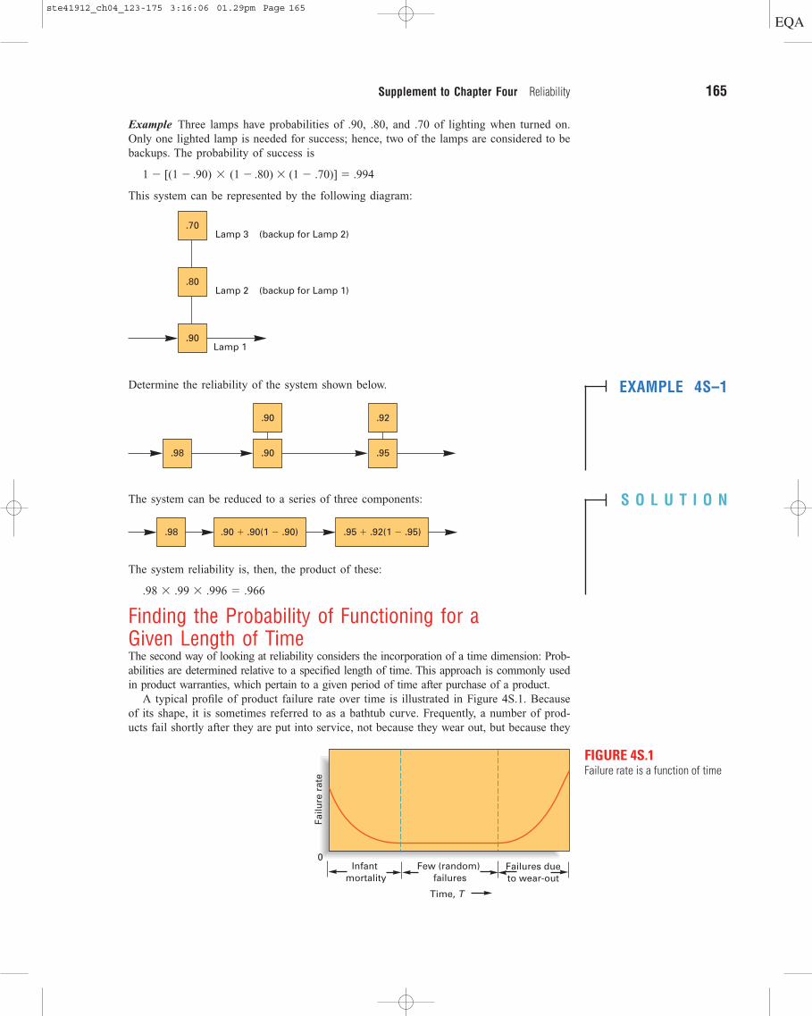
Information on the distribution and length of each phase requires the collection ofhistorical data and analysis of those data. It often turns out that the mean time betweenfailures (MTBF) in the infant mortality phase can be modeled by a negative exponentialdistribution, such as that depicted in Figure 4S.2. Equipment failures as well as product fail-ures may occur in this pattern. In such cases, the exponential distribution can be used todetermine various probabilities of interest. The probability that equipment or a product putinto service at time 0 will fail before some specified time, T, is equal to the area under thecurve between 0 and T. Reliability is specified as the probability that a product will last atleast until time T; reliability is equal to the area under the curve beyond T. (Note that thetotal area under the curve in each phase is treated as 100 percent for computational pur-poses.) Observe that as the specified length of service increases, the area under the curveto the right of that point (i.e., the reliability) decreases.

Determining values for the area under a curve to the right of a given point, T, becomesa relatively simple matter using a table of exponential values. An exponential distributionis completely described using a single parameter, the distribution mean, which reliabilityengineers often refer to as the mean time between failures. Using the symbol T to repre-sent length of service, the probability that failure will not occur before time T (i.e., the areain the right tail) is easily determined:

where

The probability that failure will occur before time T is:

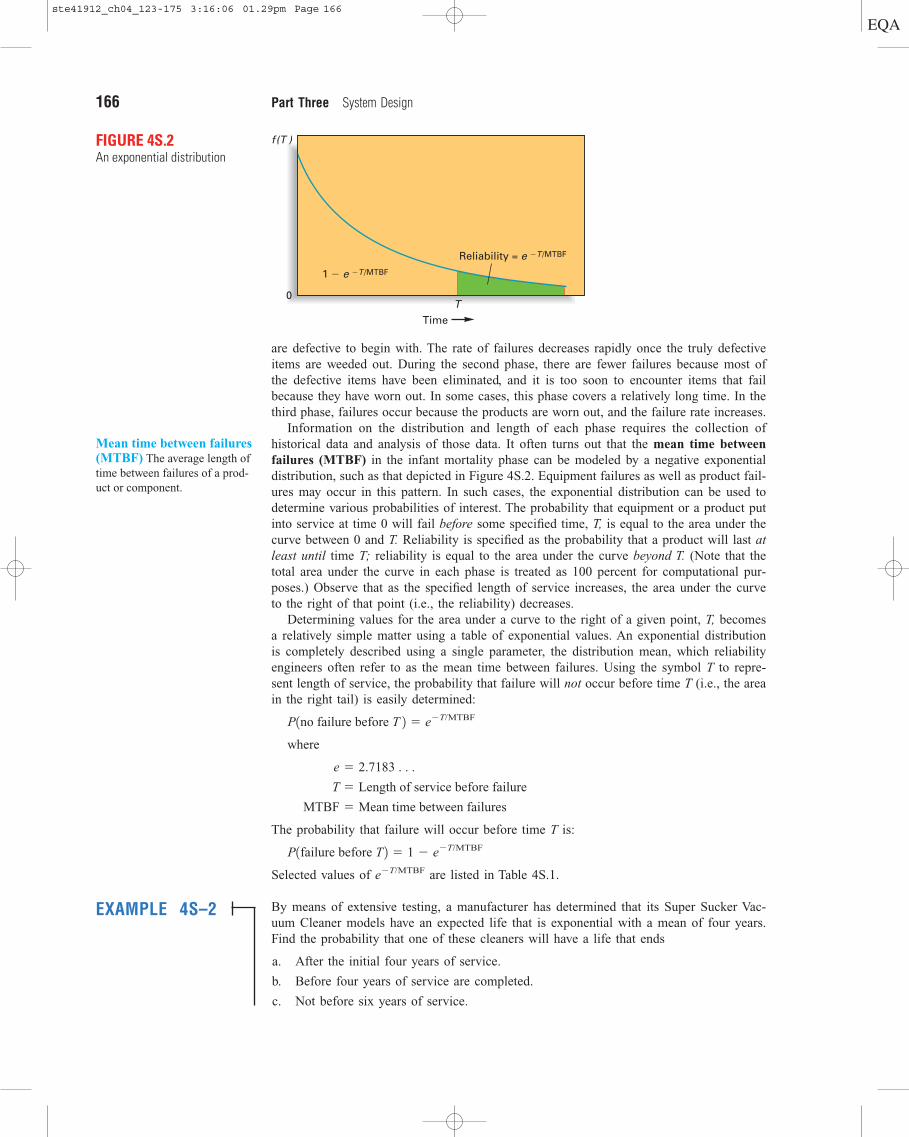
Selected values of are listed in Table 4S.1.

By means of extensive testing, a manufacturer has determined that its Super Sucker Vac-uum Cleaner models have an expected life that is exponential with a mean of four years.Find the probability that one of these cleaners will have a life that ends

a. After the initial four years of service.

b. Before four years of service are completed.

c. Not before six years of service.

e�T/MTBF

P1failure before T 2 � 1 � e�T/MTBF

MTBF � Mean time between failures

T � Length of service before failure

e � 2.7183 . . .

P1no failure before T 2 � e�T/MTBF


Mean time between failures(MTBF) The average length oftime between failures of a prod-uct or component.

TTime

Reliability = e �T /MTBF

1 � e �T /MTBF

0

f (T )FIGURE 4S.2An exponential distribution

EXAMPLE 4S–2

ste41912_ch04_123-175 3:16:06 01.29pm Page 166

a.

From Table 4S.1,

b. The probability of failure before years is or

c.

From Table 4S.1,

Product failure due to wear-out can sometimes be modeled by a normal distribution.Obtaining probabilities involves the use of a table (refer to Appendix Table B). The tableprovides areas under a normal curve from (essentially) the left end of the curve to a spec-ified point z, where z is a standardized value computed using the formula

Thus, to work with the normal distribution, it is necessary to know the mean of the distribu-tion and its standard deviation. A normal distribution is illustrated in Figure 4S.3. AppendixTable B contains normal probabilities (i.e., the area that lies to the left of z). To obtain a prob-ability that service life will not exceed some value T, compute z and refer to the table. To find

z �T � Mean wear-out time

Standard deviation of wear-out time

e�1.5 � .2231.

T/MTBF �6 years

4 years� 1.50

T � 6 years:

1 � .3679 � .6321.1 � e�1,T � 4

e�1.0 � .3679.

T/MTBF �4 years

4 years� 1.0

T � 4 years:

MTBF � 4 years


TABLE 4S.1Values of e�T/MTBFT/MTBF e�T/MTBF T/MTBF e�T/MTBF T/MTBF e�T/MTBF

0.10 .9048 2.60 .0743 5.10 .0061

0.20 .8187 2.70 .0672 5.20 .0055

0.30 .7408 2.80 .0608 5.30 .0050

0.40 .6703 2.90 .0550 5.40 .0045

0.50 .6065 3.00 .0498 5.50 .0041

0.60 .5488 3.10 .0450 5.60 .0037

0.70 .4966 3.20 .0408 5.70 .0033

0.80 .4493 3.30 .0369 5.80 .0030

0.90 .4066 3.40 .0334 5.90 .0027

1.00 .3679 3.50 .0302 6.00 .0025

1.10 .3329 3.60 .0273 6.10 .0022

1.20 .3012 3.70 .0247 6.20 .0020

1.30 .2725 3.80 .0224 6.30 .0018

1.40 .2466 3.90 .0202 6.40 .0017

1.50 .2231 4.00 .0183 6.50 .0015

1.60 .2019 4.10 .0166 6.60 .0014

1.70 .1827 4.20 .0150 6.70 .0012

1.80 .1653 4.30 .0136 6.80 .0011

1.90 .1496 4.40 .0123 6.90 .0010

2.00 .1353 4.50 .0111 7.00 .0009

2.10 .1255 4.60 .0101

2.20 .1108 4.70 .0091

2.30 .1003 4.80 .0082

2.40 .0907 4.90 .0074

2.50 .0821 5.00 .0067

S O L U T I O N

ste41912_ch04_123-175 3:16:06 01.29pm Page 167

the reliability for time T, subtract this probability from 100 percent. To obtain the value of Tthat will provide a given probability, locate the nearest probability under the curve to the leftin Table B. Then use the corresponding z in the preceding formula and solve for T.

The mean life of a certain ball bearing can be modeled using a normal distribution with amean of six years and a standard deviation of one year. Determine each of the following:

a. The probability that a ball bearing will wear out before seven years of service.

b. The probability that a ball bearing will wear out after seven years of service (i.e., findits reliability).

c. The service life that will provide a wear-out probability of 10 percent.

.

.

Wear-out life is normally distributed.

a. Compute z and use it to obtain the probability directly from Appendix Table B (seediagram).

Thus,

b. Subtract the probability determined in part a from 100 percent (see diagram).

1.00 � .8413 � .1587

P1T 6 72 � .8413.

z �7 � 6

1� � 1.00

Wear-out life standard deviation � 1 year

Wear-out life mean � 6 years


Reliability

0 zz scale

Mean life

Years

T

FIGURE 4S.3A normal curve

EXAMPLE 4S–3

0 +1.00

z scale

6

Years

7

.8413

0 +1.00

z scale

6

Years

7

.1587

S O L U T I O N

ste41912_ch04_123-175 3:16:06 01.29pm Page 168

c. Use the normal table and find the value of z that corresponds to an area under the curveof 10 percent (see diagram).

Solving for T, we find

AVAILABILITYA related measure of importance to customers, and hence to designers, is availability. Itmeasures the fraction of time a piece of equipment is expected to be operational (as opposedto being down for repairs). Availability can range from zero (never available) to 1.00 (alwaysavailable). Companies that can offer equipment with a high availability factor have a com-petitive advantage over companies that offer equipment with lower availability values. Avail-ability is a function of both the mean time between failures and the mean time to repair.The availability factor can be computed using the following formula:

where

A copier is able to operate for an average of 200 hours between repairs, and the mean repairtime is two hours. Determine the availability of the copier.

and

Two implications for design are revealed by the availability formula. One is that avail-ability increases as the mean time between failures increases. The other is that availabilityalso increases as the mean repair time decreases. It would seem obvious that designers wouldwant to design products that have a long time between failures. However, some designoptions enhance repairability, which can be incorporated into the product. Ink jet printers,for example, are designed with print cartridges that can easily be replaced.

Availability �MTBF

MTBF � MTR�

200

200 � 2� .99

MTR � 2 hoursMTBF � 200 hours

MTR � Mean time to repair

MTBF � Mean time between failures

Availability �MTBF

MTBF � MTR

T � 4.72 years.

z � �1.28 �T � 6

1


0z = �1.28

z scale

6

Years

90%

10%

4.72

Availability The fraction oftime a piece of equipment isexpected to be available foroperation.

S O L U T I O N

EXAMPLE 4S–4

KEY TERMSavailability, 169independent events, 164mean time between failures (MTBF), 166

redundancy, 164reliability, 163

ste41912_ch04_123-175 3:16:06 01.29pm Page 169

SOLVED PROBLEMS

Problem 1 A product design engineer must decide if a redundant component is cost-justified in a certain sys-tem. The system in question has a critical component with a probability of .98 of operating. Sys-tem failure would involve a cost of $20,000. For a cost of $100, a switch could be added thatwould automatically transfer the system to the backup component in the event of a failure. Shouldthe backup be added if the backup probability is also .98?

Because no probability is given for the switch, we will assume its probability of operating when neededis 100 percent. The expected cost of failure (i.e., without the backup) is

With the backup, the probability of not failing would be:

Hence, the probability of failure would be The expected cost of failure withthe backup would be the added cost of the backup component plus the failure cost:

Because this is less than the cost without the backup, it appears that adding the backup is defi-nitely cost justifiable.

Due to the extreme cost of interrupting production, a firm has two standby machines available incase a particular machine breaks down. The machine in use has a reliability of .94, and the back-ups have reliabilities of .90 and .80. In the event of a failure, either backup can be pressed intoservice. If one fails, the other backup can be used. Compute the system reliability.

and

The system can be depicted in this way:

R3 � .80R2 � .90,R1 � .94,

$100 � $20,0001.00042 � $108

1 � .9996 � .0004.

.98 � .021.982 � .9996

$20,000 � 11 � .982 � $400.Solution

Problem 2

Solution

Problem 3

Solution

Problem 4

Solution


.94

.90

.80

A hospital has three independent fire alarm systems, with reliabilities of .95, .97, and .99. In theevent of a fire, what is the probability that a warning would be given?

A warning would not be given if all three alarms failed. The probability that at least one alarmwould operate is (none operate):

A weather satellite has an expected life of 10 years from the time it is placed into earth orbit.Determine its probability of no wear-out before each of the following lengths of service. Assumethe exponential distribution is appropriate.

a. 5 years. b. 12 years. c. 20 years. d. 30 years.

MTBF � 10 years

P1warning2 � 1 � .000015 � .999985

P1none operate2 � 11 � .952 11 � .972 11 � .992 � .000015

1 � P

� .94 � .9011 � .942 � .8011 � .902 11 � .942 � .9988 Rsystem � R1 � R211 � R12 � R311 � R22 11 � R12

ste41912_ch04_123-175 3:16:06 01.29pm Page 170

Compute the ratio T/MTBF for 12, 20, and 30, and obtain the values of fromTable 4S.1. The solutions are summarized in the following table:

T MTBF T/MTBF

a. 5 10 0.50 .6065

b. 12 10 1.20 .3012

c. 20 10 2.00 .1353

d. 30 10 3.00 .0498

What is the probability that the satellite described in Solved Problem 4 will fail between 5 and 12years after being placed into earth orbit?

Using the probabilities shown in the previous solution, you obtain:

.3053

The corresponding area under the curve is illustrated as follows:

�P1failure after 12 years2 � .3012

P1failure after 5 years2 � .6065

� P1failure after 12 years2P15 years 6 failure 6 12 years2 � P1failure after 5 years2

e�T/MTBF

e�T/MTBFT � 5,

Problem 5

Solution

Problem 6

Solution


125

Years

0

f(t)

.3053

P (5 < Failure < 12)

One line of radial tires produced by a large company has a wear-out life that can be modeled usinga normal distribution with a mean of 25,000 miles and a standard deviation of 2,000 miles. Deter-mine each of the following:

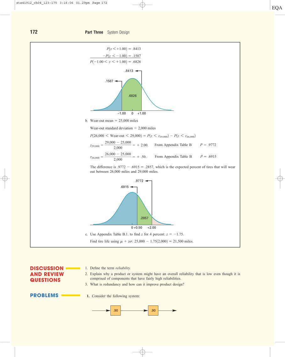
a. The percentage of tires that can be expected to wear out within miles of the average(i.e., between 23,000 miles and 27,000 miles).

b. The percentage of tires that can be expected to fail between 26,000 miles and 29,000 miles.

c. For what tire life would you expect 4 percent of the tires to have worn out?

Notes: (1) Miles are analogous to time and are handled in exactly the same way; (2) the term per-centage refers to a probability.

a. The phrase “within miles of the average” translates to within one standard deviation ofthe mean since the standard deviation equals 2,000 miles. Therefore the range of z is to , and the area under the curve between those points is found as the differencebetween and using values obtained from Appendix Table B.P1z 6 �1.002,P1z 6 �1.002

z � �1.00z � �1.00,

�2,000

�2,000

ste41912_ch04_123-175 3:16:06 01.29pm Page 171


b.

From Appendix Table B

From Appendix Table B

The difference is which is the expected percent of tires that will wearout between 26,000 miles and 29,000 miles.

c. Use Appendix Table B.1. to find z for 4 percent:

Find tire life using 25,000 � 1.7512,0002 � 21,500 miles.m � zs:

z � �1.75.

.9772 � .6915 � .2857,

P � .6915z26,000 �26,000 � 25,000

2,000� � .50.

P � .9772z29,000 �29,000 � 25,000

2,000� � 2.00.

P126,000 6 Wear-out 6 29,0002 � P1z 6 z29,0002 � P1z 6 z26,0002

Wear-out standard deviation � 2,000 miles

Wear-out mean � 25,000 miles

P1�1.00 6 z 6 �1.002 � .6826

�P1z 6 �1.002 � .1587

P1z 6 �1.002 � .8413

0 +1.00

.6826

–1.00

.1587

.8413

0 +0.50 +2.00

.6915

.9772

.2857

1. Define the term reliability.

2. Explain why a product or system might have an overall reliability that is low even though it iscomprised of components that have fairly high reliabilities.

3. What is redundancy and how can it improve product design?

1. Consider the following system:

.90 .90

DISCUSSIONAND REVIEW QUESTIONS

PROBLEMS

ste41912_ch04_123-175 3:16:06 01.29pm Page 172

a. .81b. .9801c. .9783

.9033

.9726

.93

a. .9315b. .9953c. .994

a. .7876b.

c. Add to component with .90reliability.

4th � .86643rd � .83492nd � .82701st � .8034

a. Plan 1: .9865Plan 2: .9934

b. See IM.c. space, cost, etc.

a. .0021b. .0022

Determine the probability that the system will operate under each of these conditions:a. The system as shown.b. Each system component has a backup with a probability of .90 and a switch that is 100 per-

cent reliable.c. Backups with .90 probability and a switch that is 99 percent reliable.

2. A product is composed of four parts. In order for the product to function properly in a given situa-tion, each of the parts must function. Two of the parts have a .96 probability of functioning, and twohave a probability of .99. What is the overall probability that the product will function properly?

3. A system consists of three identical components. In order for the system to perform as intended,all of the components must perform. Each has the same probability of performance. If the sys-tem is to have a .92 probability of performing, what is the minimum probability of performingneeded by each of the individual components?

4. A product engineer has developed the following equation for the cost of a system component:where C is the cost in dollars and P is the probability that the component will oper-

ate as expected. The system is composed of two identical components, both of which must oper-ate for the system to operate. The engineer can spend $173 for the two components. To the near-est two decimal places, what is the largest component probability that can be achieved?

5. The guidance system of a ship is controlled by a computer that has three major modules. In orderfor the computer to function properly, all three modules must function. Two of the modules havereliabilities of .97, and the other has a reliability of .99.a. What is the reliability of the computer?b. A backup computer identical to the one being used will be installed to improve overall relia-

bility. Assuming the new computer automatically functions if the main one fails, determinethe resulting reliability.

c. If the backup computer must be activated by a switch in the event that the first computer fails,and the switch has a reliability of .98, what is the overall reliability of the system? (Both theswitch and the backup computer must function in order for the backup to take over.)

6. One of the industrial robots designed by a leading producer of servomechanisms has four majorcomponents. Components’ reliabilities are .98, .95, .94, and .90. All of the components must func-tion in order for the robot to operate effectively.a. Compute the reliability of the robot.b. Designers want to improve the reliability by adding a backup component. Due to space limi-

tations, only one backup can be added. The backup for any component will have the samereliability as the unit for which it is the backup. Which component should get the backup inorder to achieve the highest reliability?

c. If one backup with a reliability of .92 can be added to any one of the main components, whichcomponent should get it to obtain the highest overall reliability?

7. A production line has three machines A, B, and C, with reliabilities of .99, .96, and .93, respec-tively. The machines are arranged so that if one breaks down, the others must shut down. Engi-neers are weighing two alternative designs for increasing the line’s reliability. Plan 1 involvesadding an identical backup line, and plan 2 involves providing a backup for each machine. Ineither case, three machines (A, B, and C) would be used with reliabilities equal to the origi-nal three.a. Which plan will provide the higher reliability?b. Explain why the two reliabilities are not the same.c. What other factors might enter into the decision of which plan to adopt?

8. Refer to the previous problem.a. Assume that the single switch used in plan 1 is 98 percent reliable, while reliabilities of the

machines remain the same. Recalculate the reliability of plan 1. Compare the reliability of thisplan with the reliability of plan 1 calculated in solving the original problem. How much didthe reliability of plan 1 decrease as a result of a 98 percent reliable switch?

b. Assume that the three switches used in plan 2 are all 98 percent reliable, while reliabilities ofthe machines remain the same. Recalculate the reliability of plan 2. Compare the reliabilityof this plan with the reliability of plan 2 calculated in solving the original problem. How muchdid the reliability of plan 2 decrease?

9. A Web server has five major components that must all function in order for it to operate asintended. Assuming that each component of the system has the same reliability, what is the min-imum reliability each one must have in order for the overall system to have a reliability of .98?

C � 110P22,


.996

ste41912_ch04_123-175 3:16:06 01.29pm Page 173


10. Repeat Problem 9 under the condition that one of the components will have a backup with areliability equal to that of any one of the other components.

11. Hoping to increase the chances of reaching a performance goal, the director of a research projecthas assigned three separate research teams the same task. The director estimates that the team prob-abilities are .9, .8, and .7 for successfully completing the task in the allotted time. Assuming thatthe teams work independently, what is the probability that the task will not be completed in time?

12. An electronic chess game has a useful life that is exponential with a mean of 30 months. Deter-mine each of the following:a. The probability that any given unit will operate for at least (1) 39 months, (2) 48 months,

(3) 60 months.b. The probability that any given unit will fail sooner than (1) 33 months, (2) 15 months, (3) 6

months.c. The length of service time after which the percentage of failed units will approximately equal

(1) 50 percent, (2) 85 percent, (3) 95 percent, (4) 99 percent.

13. A manufacturer of programmable calculators is attempting to determine a reasonable free-serviceperiod for a model it will introduce shortly. The manager of product testing has indicated that thecalculators have an expected life of 30 months. Assume product life can be described by an expo-nential distribution.a. If service contracts are offered for the expected life of the calculator, what percentage of those

sold would be expected to fail during the service period?b. What service period would result in a failure rate of approximately 10 percent?

14. Lucky Lumen light bulbs have an expected life that is exponentially distributed with a mean of5,000 hours. Determine the probability that one of these light bulbs will lasta. At least 6,000 hours.b. No longer than 1,000 hours.c. Between 1,000 hours and 6,000 hours.

15. Planetary Communications, Inc., intends to launch a satellite that will enhance reception of tel-evision programs in Alaska. According to its designers, the satellite will have an expected life ofsix years. Assume the exponential distribution applies. Determine the probability that it will func-tion for each of the following time periods:a. More than 9 years.b. Less than 12 years.c. More than 9 years but less than 12 years.d. At least 21 years.

16. An office manager has received a report from a consultant that includes a section on equipmentreplacement. The report indicates that scanners have a service life that is normally distributed witha mean of 41 months and a standard deviation of 4 months. On the basis of this information, deter-mine the percentage of scanners that can be expected to fail in the following time periods:a. Before 38 months of service.b. Between 40 and 45 months of service.c. Within months of the mean life.

17. A major television manufacturer has determined that its 19-inch color TV picture tubes have amean service life that can be modeled by a normal distribution with a mean of six years and astandard deviation of one-half year.a. What probability can you assign to service lives of at least (1) Five years? (2) Six years?

(3) Seven and one-half years?b. If the manufacturer offers service contracts of four years on these picture tubes, what per-

centage can be expected to fail from wear-out during the service period?

18. Refer to Problem 17. What service period would achieve an expected wear-out rate ofa. 2 percent?b. 5 percent?

19. Determine the availability for each of these cases:a.b.

20. A machine can operate for an average of 10 weeks before it needs to be overhauled, a processwhich takes two days. The machine is operated five days a week. Compute the availability of thismachine. (Hint: All times must be in the same units.)

average repair time � 6 hours.MTBF � 300 hours,average repair time � 3 days.MTBF � 40 days,

� 2

.006

a. (1): .2725(2): .2019(3): .1353

b. (1): .6671(2): .3935(3): .1813

c. (1): 21 months(2): 57 months(3): 90 months(4): 138 months

a. .6321b. 3 months

a. .3012b. .1813c. .5175

a. .2231b. .8647c. .0878d. .0302

a. 22.66%b. 44%c. 38.3%

a. (1): z � �2.00

(2):

(3): z � �3.00

� .0013 P � 13/10,000

P � .5000 z � 0.00 P � .9772

b.nearly zero

z � �4.00

.995

a.4.97 years

b.5.18 years

a. .930b. .980

z � �1.645

z � �2.055

.962

ste41912_ch04_123-175 3:16:06 01.29pm Page 174

21. A manager must decide between two machines. The manager will take into account eachmachine’s operating costs and initial costs, and its breakdown and repair times. Machine A hasa projected average operating time of 142 hours and a projected average repair time of 7 hours.Projected times for machine B are an average operating time of 65 hours and a repair time of2 hours. What are the projected availabilities of each machine?

22. A designer estimates that she can (a) increase the average time between failures of a part by5 percent at a cost of $450, or (b) reduce the average repair time by 10 percent at a cost of $200.Which option would be more cost-effective? Currently, the average time between failures is 100hours and the average repair time is 4 hours.

23. Auto batteries have an average life of 2.7 years. Battery life is normally distributed with a meanof 2.7 years and a standard deviation of .3 year. The batteries are warranted to operate for a min-imum of 2 years. If a battery fails within the warranty period, it will be replaced with a new bat-tery at no charge. The company sells and installs the batteries. Also, the usual $5 installationcharge will be waived.a. What percentage of batteries would you expect to fail before the warranty period expires?b. A competitor is offering a warranty of 30 months on its premium battery. The manager of this

company is toying with the idea of using the same battery with a different exterior, labelingit as a premium battery, and offering a 30-month warranty on it. How much more would thecompany have to charge on its “premium” battery to offset the additional cost of replacingbatteries?

c. What other factors would you take into consideration besides the price of the battery?

Machine Machine B � .970

A � .953

(a) .9633, .9653(b) yields greater availability for

less cost.

a. 1%b. $5


ste41912_ch04_123-175 3:16:06 01.29pm Page 175

Reliability - JUfilesjufiles.com/wp-content/uploads/2016/05/Reliability.pdf · system as a whole...

Documents

Transcript of Reliability - JUfilesjufiles.com/wp-content/uploads/2016/05/Reliability.pdf · system as a whole...