Reject Inference Methods in Credit Scoring: A rational review

HAL Id: hal-03087279https://hal.inria.fr/hal-03087279v2

Submitted on 31 Dec 2021

HAL is a multi-disciplinary open accessarchive for the deposit and dissemination of sci-entific research documents, whether they are pub-lished or not. The documents may come fromteaching and research institutions in France orabroad, or from public or private research centers.

L’archive ouverte pluridisciplinaire HAL, estdestinée au dépôt et à la diffusion de documentsscientifiques de niveau recherche, publiés ou non,émanant des établissements d’enseignement et derecherche français ou étrangers, des laboratoirespublics ou privés.

Reject Inference Methods in Credit ScoringAdrien Ehrhardt, Christophe Biernacki, Vincent Vandewalle, Philippe

Heinrich, Sébastien Beben

To cite this version:Adrien Ehrhardt, Christophe Biernacki, Vincent Vandewalle, Philippe Heinrich, Sébastien Beben. Re-ject Inference Methods in Credit Scoring. Journal of Applied Statistics, Taylor & Francis (Routledge),2021. �hal-03087279v2�

https://hal.inria.fr/hal-03087279v2

https://hal.archives-ouvertes.fr

APPLICATION NOTE

Reject Inference Methods in Credit Scoring

Adrien Ehrhardta and Christophe Biernackib, c and Vincent Vandewalleb, d andPhilippe Heinrichc and Sebastien Bebene

aGroupe Credit Agricole, Groupe de Recherche Operationnelle, Montrouge, France; bInria;cUniversite de Lille, Laboratoire Paul Painleve, Villeneuve d’Ascq, France; dULR 2694 -METRICS : Evaluation des technologies de sante et des pratiques medicales, F-59000 Lille,France; eBNP Paribas Personal Finance, Levallois-Perret, France.

ARTICLE HISTORY

Compiled February 23, 2021

ABSTRACT

The granting process of all credit institutions is based on the probability that theapplicant will refund his/her loan given his/her characteristics. This probability alsocalled score is learnt based on a dataset in which rejected applicants are de factoexcluded. This implies that the population on which the score is used will be di↵erentfrom the learning population. Thus, this biased learning can have consequenceson the scorecard’s relevance. Many methods dubbed “reject inference” have beendeveloped in order to try to exploit the data available from the rejected applicantsto build the score. However most of these methods are considered from an empiricalpoint of view, and there is some lack of formalization of the assumptions that arereally made, and of the theoretical properties that can be expected. In order topropose a formalization of such usually hidden assumptions for some of the mostcommon reject inference methods, we rely on the general missing data modellingparadigm. It reveals that hidden modelling is mostly incomplete, thus prohibitingto compare existing methods within the general model selection mechanism (exceptby financing “non-fundable” applicants, which is rarely performed in practice). So,we are reduced to empirically assess performance of the methods in some controlledsituations involving both some simulated data and some real data (from CreditAgricole Consumer Finance (CACF), a major European loan issuer). Unsurprisingly,no method seems uniformly dominant. Both these theoretical and empirical resultsnot only reinforce the idea to carefully use the classical reject inference methods butalso to invest in future research works for designing model-based reject inferencemethods, which allow rigorous selection methods (without financing “non-fundable”applicants).

KEYWORDSreject inference, credit risk, scoring, data augmentation, scorecard, semi-supervisedlearning

1. Introduction

Corresponding Author: Adrien Ehrhardt. Email: [email protected]

1.1. Aim of reject inference

For a new applicant’s profile and credit’s characteristics, the lender aims atestimating the repayment probability. To this end, the credit modeler fits apredictive model, often a logistic regression, between already financed clients’characteristics x = (x1, . . . , xd), here d characteristics, and their repayment status,a binary variable y 2 {0, 1} (where 1 corresponds to “good” clients and 0 to “bad”clients). The model is then applied to the new applicant and yields an estimate ofits repayment probability, called score after an increasing transformation (e.g. thelogit in the case of logistic regression). Over some cut-o↵ value of the score, theapplicant is accepted, except if further “expert” rules (e.g. credit bureauinformation, overindebtedness) or an operator come into play.

The through-the-door population (all applicants) can be classified into twocategories thanks to a binary variable z taking values in {f, nf} where f stands forfinanced applicants and nf for non-financed ones. As the repayment variable y ismissing for non-financed applicants, credit scorecards are only constructed onfinanced clients’ data but then applied to the whole through-the-door population.The relevance of this process is a natural question which is dealt in the field ofreject inference. The idea is to use the characteristics of non-financed clients in thescorecard building process to avoid a population bias, and thus to improve theprediction on the whole through-the-door population. Such methods have beendescribed in [2, 9, 19, 24] among others.

1.2. Literature review

Formalization of the reject inference problem is of first importance given thepotential financial stakes for credit organizations we previously mentioned. It hasnotably been investigated in [8] who first saw reject inference as a missing dataproblem. More precisely, it can be addressed as a part of the semi-supervisedlearning setting, which consists in learning from both labelled and unlabelled data.However, in the semi-supervised setting, it is generally assumed that labelled dataand unlabelled data come from the same distribution (see [4]), which is rarely thecase in Credit Scoring. Note that the case of a global misspecified model (both forlabelled and unlabelled data), addressed by the initial work in [11], can alsocomplicate this concern. Moreover, the main use case of semi-supervised learning iswhen the number of unlabelled data is far larger than the number of labelled data,which is not the case in Credit Scoring since the number of rejected clients andaccepted clients is often balanced and depends heavily on the financial institution,the portfolio considered, etc. Consequently, reject inference and related methodsrequire specific studies.

Recent papers (see [12], [10], [1], [14], [16], [21], [26]) proposed reject inferencetechniques for other models than the usual logistic regression on which we focushere. Some of them can be cast into the general framework we introduce inSection 2.4: we elaborate on these in Section 3.8. In a nutshell, the proposedmethods in [26], [1] and [14] use the same principle as the “Reclassification”method (Section 3.4): we show that in the case of logistic regression, this methodproduces a biased estimate. For other models however, little can be said exceptthat discarding not financed clients (see Section 3.2 and Appendix B) might indeedyield a biased model: logistic regression, being a “local” model in the sense of [27],i.e. directly modelling p(y|x), is immune (under thereafter detailed assumptions)to biasedness in x which is not the case of e.g. generative, tree-based methods, orSVMs which explicitly make use of p(x).

Moreover, the conclusions drawn in [26], [1] and [14] stem either from numericalexperiments on financed clients only, with sample weights depending on theoutcome of the loan, which might also influence the estimate’s properties, or fromfirst inferring the status of not financed clients by the proposed model itself,prohibiting the access to a true test set. We show in Section 2.5 that this isinherently flawed and warn that reporting performance metrics on rejectedapplicants for which the repayment status is inferred is deceptive. We take anopposite stance in Section 4 by simulating a stricter financing mechanism so as tosimulate rejected loans for which we know the status and thus control themissingness mechanism. However, when the model is “live” and depending on thefinancial institution, the latter is not known such that these experiments are not

2

generally conclusive either. In [12], a complex heuristic algorithm involvingXGBoost and Isolation Forest is presented without theoretical results. Empiricalresults are also given on the basis of inferred status of not financed clients.Ultimately, these methods bear the same two major flaws the usual (logisticregression-based) ones do: they are heuristics with implicit hypotheses and withouttheoretical guarantees; they cannot be empirically evaluated either sinceexperiments always rely on biased samples. In [16], a generative model, similar tothe one we use in Section 4.1 but with a richer hypothesis space, is used. Thesetypes of models, by estimating the joint distribution p(x, y) can bestraightforwardly applied to partially-labeled data, but require stronger hypotheseson the data generating mechanism which can lead to worse results thandiscriminative models, as we show. However, generative models are probably themost promising in reject inference, since they can be evaluated on informationcriteria (Section 2.4) and are semi-supervised “out-of-the-box” in contrast withsupervised methods which require some heuristics to first infer a label for rejectedclients.

1.3. Outline of the paper

The purpose of the present paper is thus to revisit most widespread rejectinference methods in order to clarify which mathematical hypotheses, if any,underlie these heuristics. This rational review is a fundamental step for raisingclear conclusions on their relevance. The question of retaining a reject inferencemethod has also to be addressed in a formal way, namely in the general modelselection paradigm.

The outline of the paper is the following. In Section 2, we recast the rejectinference concern as a missing data problem embedded in a general parametricmodelling. It allows to discuss related missing data mechanisms, a standardlikelihood-based estimation process and also some possible model selectionstrategies. In Section 3, the most common reject inference methods are describedand their mathematical properties are exhibited. These latter mostly rely on themissing data framework previously introduced in Section 2. However, we show thatsuch a theoretical understanding cannot assess the expected quality of the scoreprovided by each method. Subsequently, each method is empirically tested andcompared on simulated and real data from CACF in Section 4 to illustrate that nomethod is universally superior. Finally, some guidelines are given to bothpractitioners (when using existing reject inference methods) and statisticians(when designing new reject inference methods) in Section 5.

2. Credit Scoring modelling

2.1. Data

The decision process of financial institutions to accept a credit application is easilyembedded in the probabilistic framework. The latter o↵ers rigorous tools for takinginto account both the variability of applicants and the uncertainty on their abilityto pay back the loan. In this context, the important term is p(y|x), designating theprobability that a new applicant (described by his characteristics x) will pay backhis loan (y = 1) or not (y = 0). Estimating p(y|x) is thus an essential task of anyCredit Scoring process.

To perform estimation, a specific n-sample (the observed sample) T is available,decomposed into two disjoint and meaningful subsets, denoted by Tf and Tnf

(T = Tf [ Tnf, Tf \ Tnf = ;). The first subset (Tf) corresponds to applicantsxi = (xi,1, . . . , xi,d), described by d features, who have been financed (zi = f) and,consequently, for whom the repayment status yi is known. With their respectivenotation xf = {xi}i2F, yf = {yi}i2F and zf = {zi}i2F, where F = {i : zi = f}denotes the corresponding subset of indexes, we have thus Tf = {xf,yf, zf}. Thesecond subset (Tnf) corresponds to other applicants xi who have not been financed(zi = nf) and, consequently, for who the repayment status yi is unknown. Withtheir respective notation xnf = {xi}i2NF, ynf = {yi}i2NF and znf = {zi}i2NF,where NF = {i : zi = nf} denotes the corresponding subset of indexes, we havethus Tnf = {xnf, znf}. We notice that yi values (i 2 NF) are excluded from theobserved sample Tnf, since they are missing. Finally, the following notation will bealso used: x = {xf,xnf}.

It should be noticed that we use the “financed” versus “not financed”

3

terminology whereas most previous work use “accepted” versus “rejected” clients.Indeed, these two concepts are di↵erent: one might be accepted, but never returnthe contract and / or supporting documents, thus being not financed and yieldinga missing label y (this client might have had a better o↵er elsewhere). Also, a“rejected” client, be it by the score, or specific rules, might be (manually) financedby an operator, who might have had “proof” that the client is good. In these twocases, the common assumption that rejected clients would be performing worsethan accepted ones, all else being equal, is false. As discussed in Section 3.7, thesekinds of unverifiable assumptions fail to generalize from one financial institution toanother. We thus make no distinction inside the “not financed” population in whatfollows.

2.2. General parametric model

Estimation of p(y|x) has to rely on modelling since the true probabilitydistribution is unknown. Firstly, it is both convenient and realistic to assume thattriplets in the complete sample Tc = {xi, yi, zi}1in are all independent andidentically distributed (i.i.d.), including the unknown values of yi when i 2 NF.Secondly, it is usual and convenient to assume that the unknown distributionp(y|x) belongs to a given parametric family {p✓(y|x)}✓2⇥, where ⇥ is theparameter space. For instance, logistic regression is often considered in practice,even if we will be more general in this section. However, logistic regression will beimportant for other sections since some standard reject inference methods arespecific to this family (Section 3) and numerical experiments (Section 4) willimplement them.

As in any missing data situation (here z indicates if y is observed or not), therelative modelling process, namely p(z|x, y), has also to be clarified. Forconvenience, we can also consider a parametric family {p�(z|x, y)}�2�, where �denotes the parameter and � the associated parameter space of the financingmechanism. Note that we consider here the most general missing data situation,namely a Missing Not At Random (MNAR) mechanism (see [15]). It means that zcan be stochastically dependent on some missing data y, i.e. p(z|x, y) 6= p(z|x).We will discuss this fact in Section 2.4.

Finally, combining both previous distributions p✓(y|x) and p�(z|x, y) leads toexpress the joint distribution of (y, z) conditionally to x as:

p�(y, z|x) = p�(�)(z|y,x)p✓(�)(y|x) (1)

where {p�(y, z|x)}�2� denotes a distribution family indexed by a parameter �evolving in a space �. Here it is clearly expressed that both parameters � and ✓can depend on �, even if in the following we will note shortly � = �(�) and✓ = ✓(�). In this very general missing data situation, the missing process is said tobe non-ignorable, meaning that parameters � and ✓ can be functionally dependent(thus � 6= (�,✓)). We also discuss this fact in Section 2.4.

2.3. Maximum likelihood estimation

Mixing previous model and data, the maximum likelihood (ML) principle can beinvoked for estimating the whole parameter �, thus yielding as a by-product anestimate of the parameter ✓. Indeed, ✓ is of particular interest, the goal of thefinancial institutions being solely to obtain an estimate of p✓(y|x). The observedlog-likelihood can be written as:

`(�; T ) =X

i2F

ln p�(yi, f|xi) +X

i02NF

ln

2

4X

y2{0,1}

p�(y, nf|xi0)

3

5 . (2)

Within this missing data paradigm, the Expectation-Maximization (EM)algorithm (see [5]) can be used: it aims at maximizing the expectation of thecomplete likelihood `c(�; Tc) (defined hereafter) over the missing labels. Starting

4

from an initial value �(0), iteration (s) of the algorithm is decomposed into thefollowing two classical steps:

E-step: compute the conditional probabilities of missing yi values (i 2 NF):

y(s)i = p✓(�(s�1))(1|xi, nf) =

p�(s�1)(1, nf |xi)Py02{0,1} p�(s�1)(y0, nf |xi)

; (3)

M-step: maximize the conditional expectation of the complete log-likelihood:

`c(�; Tc) =nX

i=1

ln p�(yi, zi|xi) =X

i2F

ln p�(yi, f |xi) +X

i2NF

ln p�(yi0 , nf |xi0), (4)

leading to:

�(s) = argmax�2�

Eynf[`c(�; Tc)|T ,�(s�1)]

= argmax�2�

X

i2F

ln p�(yi, f |xi) +X

i02NF

X

y2{0,1}

y(s)i0 ln p�(y, nf |xi0).

Usually, stopping rules rely either on a predefined number of iterations, or on apredefined stability criterion of the observed log-likelihood.

2.4. Some current restrictive missingness mechanisms

The latter parametric family is very general since it considers both that themissingness mechanism is MNAR and non-ignorable. But in practice, it is commonto consider ignorable models for the sake of simplicity, meaning that � = (�,✓).Missingness mechanisms and ignorability are more formally defined inAppendix A. There exists also some restrictions to the MNAR mechanism.

The first restriction to MNAR is the Missing Completely At Random (MCAR)setting, meaning that p(z|x, y) = p(z). In that case, applicants should be acceptedor rejected without taking into account their descriptors x. Such a process is notrealistic at all for representing the actual process followed by financial institutions.Consequently it is always discarded in Credit Scoring.

The second restriction to MNAR is the Missing At Random (MAR) setting,meaning that p(z|x, y) = p(z|x). The MAR missingness mechanism seems realisticfor Credit Scoring applications, for example when financing is based solely on afunction of x, e.g. in the case of a score associated to a cut-o↵, provided all clients’characteristics of this existing score are included in x. It is a usual assumption inCredit Scoring even if, in practice, the financing mechanism may depend also onunobserved features (thus not present in x), which is particularly true when anoperator adds a subjective, often intangible, expertise. In the MAR situation thelog-likelihood (2) can be reduced to:

`(�; T ) = `(✓; Tf) +nX

i=1

ln p�(zi|xi), (5)

with `(✓; Tf) =P

i2F ln p✓(yi|xi). Combining it with the ignorable assumption,estimation of ✓ relies only on the first part `(✓; Tf), since the value � has noinfluence on ✓. In that case, invoking an EM algorithm due to missing data y is nolonger required as will be made explicit in Section 3.2.

2.5. Model selection

At this step, several kinds of parametric model (1) have been assumed. It concernsobviously the parametric family {p✓(y|x)}✓2⇥, and also the missingnessmechanism MAR or MNAR. However, it has to be noticed that MAR versus

5

MNAR cannot be tested since we do not have access to y for non-financed clients(see [18]). However, model selection is possible by modelling also the wholefinancing mechanism, namely the family {p�(z|x, y)}�2�.

Scoring for credit application can be recast as a semi-supervised classificationproblem (see [4] for a thorough reference). In this case, following works in [23],classical model selection criteria can be divided into two categories: either scoringperformance criteria as e.g. error rate on a test set T test, or information criterialike e.g. the Bayesian Information Criterion (BIC).

In the category of error rate criteria, the typical error rate is expressed asfollows:

Error(T test) =1

|T test|X

i2T test

I(yi 6= yi), (6)

where T test is an i.i.d. test sample from p(y|x) and where yi is the estimated valueof the related yi value involved by the estimated model at hand. The model leadingto the lowest error value is then retained. However, in the Credit Scoring contextthis criterion family is not available since no sample T test is itself available. Thisproblem can be exhibited through the following straightforward expression

p(y|x) =X

z2{f,nf}

p(y|x, z)p(z|x) (7)

where p(y|x, z) is unknown and p(z|x) is known since this latter is implicitlydefined by the financial institution itself. We notice that obtaining a sample fromp(y|x) would require that the financial institution draws ztest i.i.d. from p(z|x)before observing the results ytest i.i.d. from p(y|x, z). But in practice it isobviously not the case, a threshold being applied to the distribution p(z|x) forretaining only a set of fundable applicants, the non-fundable applicants beingdefinitively discarded, preventing us from getting a test sample T test from p(y|x).As a matter of fact, only a sample T test

f of p(y|x, f) is available, irrevocablyprohibiting the calculus of (6) as a model selection criterion.

In the category of information criteria, the BIC criterion is expressed as thefollowing penalization of the maximum log-likelihood:

BIC = �2`(�; T ) + dim(�) lnn, (8)

where � is the maximum likelihood estimate (MLE) of � and dim(�) is thenumber of parameters to be estimated in the model at hand. The model leading tothe lowest BIC value is then retained. Many other BIC-like criteria exist (see [23])but the underlined idea is unchanged. Contrary to the error rate criteria like (6), itis thus possible to compare models without funding “non-fundable applicants”since only the available sample T is required. However, computing (8) requires toprecisely express the model families {p�(y, z|x)}�2� which compete.

2.6. Reject inference heuristics

Proposed reject inference methods are not usually examined through the modelselection lens, as presented in the previous section; they are heuristics consisting inalgorithms inferring the label y of non-financed clients, which make the use ofclassical supervised methods possible on the whole dataset. However and as seen inthe previous section, failing to compare them on a test set where both populationsare financed make empirical results superfluous. Consequently, we focus in the nextsection on formalizing the implicit hypotheses which underlie these heuristics anddraw theoretical conclusions on which methods shall work in practice depending onthe missingness mechanism. We focus on most widespread methods for logisticregression, however, as promised in our literature review, without loss of generality,and state in Section 3.8 how more recent approaches (see Section 1.2) based onother methods integrate with this framework.

6

3. Rational reinterpretation of reject inference methods

3.1. The reject inference challenge

As discussed in the previous section, a rigorous way to use the whole observedsample T in the estimation process implies some challenging modelling andassumption steps. A method using the whole sample T is traditionally called areject inference method since it uses not only financed applicants (sample Tf) butalso non-financed, or rejected, applicants (sample Tnf). Since modelling thefinancing mechanism p(z|x, y) is sometimes a too heavy task, such methodspropose alternatively to use the whole sample T in a more empirical manner.However, this is somehow a risky strategy since we have also seen in the previoussection that validating methods with error rate like criteria is not possible throughthe standard Credit Scoring process. As a result, some strategies are proposed toperform a “good” score function estimation without access to their realperformance, including ignoring non-financed clients as is usually done.

Nevertheless, most of the proposed reject inference strategies have hiddenassumptions on the modelling process. Our present challenge is to reveal as far aspossible such hidden assumptions to then discuss how realistic these are, if we failto compare them by the model selection principle.

3.2. Strategy 1: ignoring non-financed clients

3.2.1. Definition

The simplest reject inference strategy is to ignore non-financed clients forestimating ✓. Thus it consists in estimating ✓ by maximizing the log-likelihood`(✓; Tf).

3.2.2. Missing data reformulation

In fact, this strategy is equivalent to using the whole sample T (financed andnon-financed applicants) under both the MAR and ignorable assumptions. See therelated explanation in Section 2.4 and works in [27]. Consequently, this strategy istruly a particular “reject inference” strategy although it does not seem to be.

3.2.3. Estimate property

Denoting by ✓f and ✓ the MLE of `(✓; Tf) and `(✓; Tc), respectively, provided weknow yi for i 2 NF, classical ML properties (see [25] and [27]) yield under awell-specified model hypothesis (there exists ✓? s.t. p(y|x) = p✓?(y|x) for all(x, y)) and a MAR ignorable missingness mechanism that ✓ ⇡ ✓f for large enoughsamples Tf and T .

3.3. Strategy 2: Fuzzy Augmentation

3.3.1. Definition

This strategy can be found in [19] and is developed in depth in Appendix C.1. Itcorresponds to an algorithm which is starting with ✓(0) = ✓f (see previous section).

Then, all {yi}i2NF are imputed by their expected value given by: y(1)i = p✓(0)(1|xi)

(notice that these imputed values are not in {0, 1} but in ]0, 1[). The complete

log-likelihood `c(✓; T (1)c ) given in (4) in a broader context with T (1)

c = T [ y(1)nf is

maximized, with y(1)nf = {y(1)

i }i2NF, and yields final parameter estimate ✓(1).

7


Following the notations introduced in Section 2.3, and recalling that this methoddoes not take into account the financing mechanism p(z|x, y), this methodcorresponds to a unique iteration of an EM-algorithm yielding✓(1) = argmax✓ Eynf

[`c(✓; T (1)c )|T , ✓(0)]. Since � is not involved in this process, we

first deduce from Section 2.4 that, again, MAR and ignorable assumptions arepresent.


Some straightforward algebra (solving the M-step of the related EM algorithm)

allow to obtain that argmax✓ `c(✓; T(1)c ) = ✓f, regardless of any assumption on the

missingness mechanism or the true model hypothesis. In other words we have✓(1) = ✓f, so that this method is strictly equivalent to the scorecard learnt on thefinanced clients (Strategy 1 described in Section 3.2).

3.4. Strategy 3: Reclassification

3.4.1. Definition

This strategy corresponds to an algorithm which is starting with ✓(0) = ✓f (seeSection 3.2). Then, all {yi}i2NF are imputed by the maximum a posteriori (MAP)

principle given by: y(1)i = argmaxy2{0,1} p✓(0)(y|xi). The complete log-likelihood

`c(✓; T (1)c ) given in (4) in a broader context with T (1)

c = T [ y(1)nf , with

y(1)nf = {y(1)

i }i2NF, is maximized and yields parameter estimate ✓(1).

Its first variant stops at this value ✓(1). Its second variant iterates until potentialconvergence of the parameter sequence (✓(s)), after alternating s iterations

between ✓(s) and y(s)nf in a similar way as described above for the first iteration

s = 1. In practice and for logistic regression, this method can be found in [9] underthe name “Iterative Reclassification”, in [24] under the name “Reclassification” orunder the name “Extrapolation” in [2]. It is developed in depth in Appendix C.2.


This algorithm is equivalent to the so-called Classification-EM algorithm where aClassification (or MAP) step is inserted between the Expectation andMaximization steps of an EM algorithm (described in Section 2.3).Classification-EM aims at maximizing the complete log-likelihood `c(✓; Tc) overboth ✓ and ynf. Since � is not involved in this process, we first deduce fromSection 2.4 that, again, MAR and ignorable assumptions are present.


Standard properties of the estimate maximizing the complete likelihood indicatethat it is not a consistent estimate of ✓ according to [3], contrary to the traditionalML one. The related Classification-EM algorithm is also known for “sharpening”the decision boundary: predicted probabilities are closer to 0 and 1 than their truevalues as is illustrated from simulated data with a MAR ignorable mechanism onFigure 1. The scorecard ✓f on financed clients (in green) is asymptoticallyconsistent as was emphasized in Section 3.2 while the reclassified scorecard (in red)is biased even asymptotically.

3.4.3.1. Experimental setup of Figure 1 . The setup is similar tothe experiment of Section 4.1.1 with d = 1 and a single simulated cutpoint: wedraw 1 dataset of 10,000 observations of continuous data, homoscedastic andnormally distributed s.t. Y s B( 12 ) and X|Y = y s N (y, 1). We learn a logistic

regression of coe�cient ✓ and consider that rejected clients (xnf) correspond to the

8

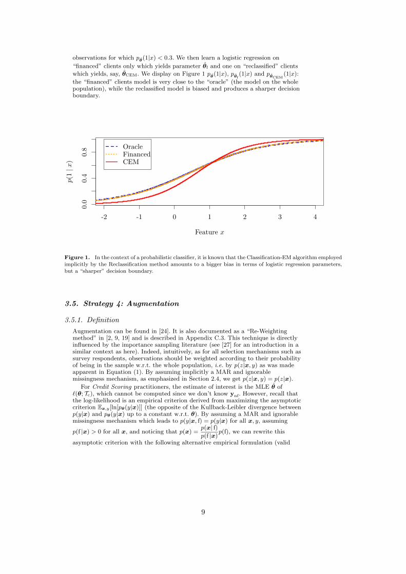
observations for which p✓(1|x) < 0.3. We then learn a logistic regression on

“financed” clients only which yields parameter ✓f and one on “reclassified” clientswhich yields, say, ✓CEM. We display on Figure 1 p✓(1|x), p✓f

(1|x) and p✓CEM(1|x):

the “financed” clients model is very close to the “oracle” (the model on the wholepopulation), while the reclassified model is biased and produces a sharper decisionboundary.

-2 -1 0 1 2 3 4

0.0

0.4

0.8

Feature x

p(1|x

)

OracleFinancedCEM

Figure 1. In the context of a probabilistic classifier, it is known that the Classification-EM algorithm employedimplicitly by the Reclassification method amounts to a bigger bias in terms of logistic regression parameters,but a “sharper” decision boundary.

3.5. Strategy 4: Augmentation

3.5.1. Definition

Augmentation can be found in [24]. It is also documented as a “Re-Weightingmethod” in [2, 9, 19] and is described in Appendix C.3. This technique is directlyinfluenced by the importance sampling literature (see [27] for an introduction in asimilar context as here). Indeed, intuitively, as for all selection mechanisms such assurvey respondents, observations should be weighted according to their probabilityof being in the sample w.r.t. the whole population, i.e. by p(z|x, y) as was madeapparent in Equation (1). By assuming implicitly a MAR and ignorablemissingness mechanism, as emphasized in Section 2.4, we get p(z|x, y) = p(z|x).

For Credit Scoring practitioners, the estimate of interest is the MLE ✓ of`(✓; Tc), which cannot be computed since we don’t know ynf. However, recall thatthe log-likelihood is an empirical criterion derived from maximizing the asymptoticcriterion Ex,y[ln[p✓(y|x)]] (the opposite of the Kullback-Leibler divergence betweenp(y|x) and p✓(y|x) up to a constant w.r.t. ✓). By assuming a MAR and ignorablemissingness mechanism which leads to p(y|x, f) = p(y|x) for all x, y, assuming

p(f |x) > 0 for all x, and noticing that p(x) =p(x| f)p(f |x)p(f), we can rewrite this

asymptotic criterion with the following alternative empirical formulation (valid

9

when n ! 1; recall we denote by X the space of x):

Ex,y[ln[p✓(y|x)]] =1X

y=0

Z

Xln p✓(y|x)p(y|x)p(x)dx

=1X

y=0

Z

Xp(f) ln p✓(y|x)

p(x| f)p(f |x)p(y|x)dx

= p(f)1X

y=0

Z

X

ln p✓(y|x)p(f |x) p(x, y| f)dx

⇡ p(f)n

X

i2F

1p(f |xi)

ln p✓(yi|xi). (9)

Recall that the summation over i 2 F means our observations (xi, yi) are drawnfrom p(x, y| f), which are precisely the ones we have at hand. Advantage of thisnew likelihood expression is that, had we access to p(f |x), the parametermaximizing this likelihood would asymptotically be equal to the MLE ✓maximizing the “classical” log-likelihood `(✓; Tc). However, p(f |x) must beestimated by any method retained by the practitioner, which can be a challengingtask by itself. In practice, the usual way is to propose to bin observations in T inK equal-length intervals of the score given by p✓f

(1|x) (often K = 10) and then tosimply estimate p(z|x) as the proportion of financed clients in each of these bins.The inverse of this estimate is then used to weight financed clients in Tf and finallythe score model is retrained within this new context (see again Appendix C.3 forall the detailed procedure).


The method aims at correcting for the selection procedure yielding the trainingdata Tf in the MAR case. As was argued in Section 3.2, if the model iswell-specified, such a procedure is superfluous as the estimated parameter ✓f isconsistent. In the misspecified case however, ✓f does not converge to the parameterof the best logistic regression approximation p✓?(y|x) of p(y|x) w.r.t. theaforementioned asymptotic criterion, contrary to the parameter given by thismethod by construction.


The importance sampling paradigm requires p(f |x) > 0 for all x, to ensure finitevariance of the targeted estimate, which is clearly not the case here: for example,jobless people are never financed. In practice, it is also unclear if the apparentbenefit of this method, all assumptions being met, is not o↵set by the addedestimation procedure of p(f |x) which remains challenging by itself.

3.6. Strategy 5: Twins

3.6.1. Definition

This reject inference method is documented internally at CACF and inAppendix C.4. It consists in combining two logistic regression-based scorecards:one predicting y learnt on financed clients (denoted by ✓f as previously), the otherpredicting z learnt on all applicants (denoted by �), before learning the finalscorecard using the predictions made by both previous scorecards on financedclients. The detailed procedure is provided in Appendix C.4.

10


The method aims at re-injecting information about the financing mechanism in theMAR non-ignorable missingness mechanism by estimating � as a logisticregression on all applicants, calculating scores (1,x)0✓f and (1,x)0� and use theseas two continuous features in a third logistic regression predicting again therepayment feature y, thus using only financed clients in Tf.


From the log-likelihood (C1) of Appendix C.4, it can be straightforwardly noticedthat the logit of p✓(yi|(1,xi)

0✓f, (1,xi)0�f) is simply a linear combination of x,

since both (1,xi)0✓f and (1,xi)

0�f are themselves a linear combination of x.Consequently, we strictly obtain ✓twins = ✓f. Finally, the last step of the Twinsmethod is known to let the scorecard estimated unchanged (it corresponds to theFuzzy Augmentation method, see Section 3.3), which allows to conclude thatTwins method is strictly identical to the financed clients method given inSection 3.2 (it provides a final scorecard ✓f).

3.7. Strategy 6: Parcelling

3.7.1. Definition

The parcelling method can be found in works in [2, 9, 24]. It is also described inAppendix C.5. This method aims to correct the log-likelihood estimation in theMNAR case by making further assumptions on p(y|x, z). It is a little deviationfrom the Fuzzy Augmentation method (Section 3.3) in a MNAR setting, where the

payment status y(1)i for non-financed clients (i 2 NF) is estimated by a quantity

now di↵ering from this one associated to financed clients (which was namelyp✓(0)(1|xi, f), with ✓(0) = ✓f). The core idea is to propose an estimate

y(1)i = p(1|xi, nf) = 1� p(0|xi, nf), for i 2 NF, with

p(0|xi, nf) / ✏k(xi)p✓(0)(0|xi, f),

where k(x) is the scoreband index among K equal-length scorebands B1, . . . , BK

(see Step (b) in Appendix C.3) and ✏1, . . . , ✏K are so-called “prudence factors”.These latter are generally such that 1 < ✏1 < · · · < ✏K , and they aim tocounterbalance the fact that non-financed low refunding probability clients areconsidered way riskier, all other things being equal, than their financedcounterparts. All these ✏k values have to be fixed by the practitioner. The methodis thereafter strictly equivalent to Fuzzy Reclassification by maximizing over ✓ thecomplete log-likelihood `c(✓; T (1)

c ) with T (1)c = T [ y(1)

nf and y(1)nf = {y(1)

i }i2NF. It

yields a final parameter estimate ✓(1).


By considering not-financed clients as riskier than financed clients with the samelevel of score, i.e. p(0|x, nf) > p(0|x, f), it is implicitly assumed that operators thatmight have interfered with the system’s decision have access to additionalinformation, say x such as supporting documents, that influence the outcome yeven when x is accounted for. In this setting, rejected and accepted clients withthe same score di↵er only by x, to which we do not have access and is accountedfor “quantitatively” in a user-defined prudence factor ✏ = (✏1, . . . , ✏K) stating thatrejected clients would have been riskier than accepted ones.


The prudence factor encompasses the practitioner’s belief about the e↵ectivenessof the operators’ rejections. It cannot be estimated from the data nor tested and is

11

consequently a matter of unverifiable expert knowledge.

3.8. Other methods related to previous strategies

In [26], [1], and [14] the “Reclassification” scheme (Section 3.4) is used inconjunction with LightGBM (and isolation forests for reject inference), Bayesiannetworks and SVMs respectively. In all three cases, “global” models (in the senseof [27]) are used. Since these rely on an estimate of p(x) at some point to obtain anestimate p(y|x), the first model, called ✓(0) in Section 3.4, used to infer theoutcome of rejected applications, is biased. By how much this biasedness willimpact the performance of the proposed method on the through-the-doorpopulation Tc w.r.t. the financed clients cannot be computed and is highlydata-dependent. Additionally and as seen with logistic regression in Section 3.4which results hold for other “local” models, the subsequent steps of the“Reclassification” procedure (referred to as ✓(s)) introduce bias on their own byimputing the labels ynf via the MAP principle (or the isolation forest for [26]): ascredit scoring datasets are relatively imbalanced (few defaults), the defaultprobability is relatively low. Consequently the MAP label of most (if not all)rejects is a “good” outcome. This yields a biased and “sharper” decision boundaryas detailed in Section 3.4.3.1.

4. Numerical experiments

Several authors compared the previously defined reject inference methods throughexperiments without concluding on what method is best and why, or if so, theirresults were in contradiction with some other works. For example, it is concludedin [2, 24] that reject inference techniques could not improve credit scorecards.In [9, 19], the opposite is stated. This emphasizes the heuristical nature of thesemethods, the absence of theoretical guarantees and consequently the fact that thesuperiority of a method on the others is highly data-dependent. In the previoussection, we showed that in theory no reject inference method produces auniversally better estimator than the financed clients model ✓f (Section 3.2). Tosupport these theoretical findings, we first use simulated data to control underwhich assumptions (missingness mechanism and well-specified model) we operate.Then we use real data from CACF where we simulate rejected applicants amongthe financed clients.

4.1. Simulated data

4.1.1. Results for MAR and well-specified model case

We draw 20 learning and 1 test datasets of 10,000 and 100,000 observationsrespectively of continuous data, homoscedastic and normally distributed s.t.Y s B( 12 ) and X|Y = y s N (µy, 2I) for y 2 {0, 1} with µ0 = 0, µ1 = 1, and

where I denotes the identity matrix. For each learning dataset, we first estimate ✓using all observations. Then, we hide yi by progressively raising the simulatedcut-o↵ defining Z = f if p✓(1|xi) > cut , and Z = nf otherwise. For each cut-o↵value cut and for each training set, all reject inference methods are trained and werepresent their mean Gini (common performance metric in Credit Scoringproportional to the Area Under the ROC Curve - higher is better).

This setting is equivalent to a MAR and ignorable missingness mechanism.Logistic regression is well-specified, such that, following our findings in Section 3,we naturally obtained the exact same results from three methods: the logisticregression on financed clients only, the logistic regression using FuzzyAugmentation and the logistic regression using the Twins method (Strategies 1, 2and 5 respectively).

We are left with the following four models displayed on Figure 2 and calculatedwith d = 8: the logistic regression on financed clients only, the logistic regressionon reclassified data, the logistic regression on augmented data and the logisticregression on parceled data with 10 equal-width score-bands and ✏k = 1.15 for

12

Cut-o↵ value

Ginion

test

set

0 0.2 0.4 0.6 0.8

0.77

0.78

0.79

0.8

0.81

0.82

0.83

0.84

0.85

Logistic regressionAugmentationReclassificationParcellingGaussian mixture

Figure 2. Comparison of reject inference methods with a well-specified model.

1 k K (common in-house practice), corresponding to Strategies 1, 3, 4 and 6respectively.

What can be concluded from Figure 2 is that logistic regression on financedclients is fine as expected. It is not statistically di↵erent from the reclassifieddataset and it is significantly better than reject inference using augmented orparceled data as the cut becomes larger.

To challenge logistic regression with a “natural” semi-supervised learningapproach, we used generative models in the form of Gaussian mixtures (i.e.X|Y = y s N (µy,⌃y) - see [17] for an introduction) for continuous features andmultinomial mixtures for categorical ones (see Appendix B for technicalities).

The Gaussian mixture model is not only as good as logistic regression on theleft side of Figure 2, all observations being labeled, which was to be expected sinceit is also well-specified and subsequently benefits from a smaller asymptoticalvariance (see [6, 20]), but it becomes better than logistic regression-based modelswhen the cut-o↵ becomes larger. This is due to their native use of unlabeled dataas detailed in Section 3.

4.1.2. Results for MAR and misspecified model case

In Section 3, we saw that in the MAR and misspecified model case, if some clientsbeneath the cut-o↵ are accepted so that for all x, p(f|x) > 0 then theAugmentation method is well-suited. However, as financing is deterministic here(recall we defined Z = f if p✓(1|xi) > cut, and Z = nf otherwise), this assumptiondoes not hold. To show numerically the consequences of misspecification, wereproduced the same experience as in the previous section, but this time usingdi↵erent variance-covariance matrices for each population (i.e.X|Y = y s N (µy,⌃y) by drawing two random positive definite matrices ⌃y fory 2 {0, 1}1). In this situation, logistic regression is misspecified whereas theGaussian mixture remains well-specified. Results are displayed on Figure 3. Thegap between logistic regression-based models and the generative model at thebeginning of the curve is a clear sign of misspecification for logistic regression.Among logistic regression-based models, the financed clients performed best, the

1Using the proposed implementation at: https://stat.ethz.ch/pipermail/r-help/2008-February/153708

13

Cut-o↵ value

Ginion

test

set

0 0.2 0.4 0.6 0.8

0.74

0.76

0.78

0.8

0.82

0.84

0.86

0.88

0.9

0.92

Logistic regressionAugmentationReclassificationParcellingGaussian mixture

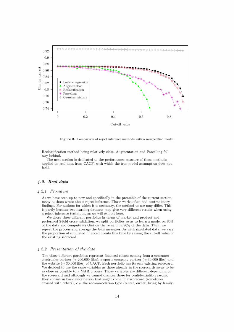
Figure 3. Comparison of reject inference methods with a misspecified model.

Reclassification method being relatively close. Augmentation and Parcelling fallway behind.

The next section is dedicated to the performance measure of those methodsapplied on real data from CACF, with which the true model assumption does nothold.

4.2. Real data

4.2.1. Procedure

As we have seen up to now and specifically in the preamble of the current section,many authors wrote about reject inference. Those works often had contradictoryfindings. For authors for which it is necessary, the method to use may di↵er. Thisis partly because two learning datasets may give very di↵erent results when usinga reject inference technique, as we will exhibit here.

We chose three di↵erent portfolios in terms of market and product andperformed 5-fold cross-validation: we split portfolios so as to learn a model on 80%of the data and compute its Gini on the remaining 20% of the data. Then, werepeat the process and average the Gini measures. As with simulated data, we varythe proportion of simulated financed clients this time by raising the cut-o↵ value ofthe existing scorecard.

4.2.2. Presentation of the data

The three di↵erent portfolios represent financed clients coming from a consumerelectronics partner (⇡ 200,000 files), a sports company partner (⇡ 30,000 files) andthe website (⇡ 30,000 files) of CACF. Each portfolio has its own existing scorecard.We decided to use the same variables as those already in the scorecards so as to beas close as possible to a MAR process. Those variables are di↵erent depending onthe scorecard and although we cannot disclose those for confidentiality reasons,they consist in basic information that might come in a scorecard (sometimescrossed with others), e.g. the accommodation type (renter, owner, living by family,

14

Rejection rate (above current level)

Ginion

test

set

0 0.1 0.2 0.3 0.4

0.25

0.3

0.35

0.4

0.45

0.5

0.55

0.6

Logistic regressionAugmentationReclassificationParcellingGenerative model

Figure 4. Comparison of several reject inference techniques for the consumer electronics dataset.

. . . ), the marital status, the age, information on eventual cosigner, etc.Note that there are both categorical and continuous variables. One common

practice in the field of Credit Scoring is to discretize every continuous variable andgroup categorical features’ levels, if numerous. Again, as we used variables alreadyin the existing scorecard, they are all categorical with 3 to 7 factor levelsdepending on the variable of interest. Depending on the dataset, there containapproximately 2 to 6% of “bad” clients.

4.2.3. Results

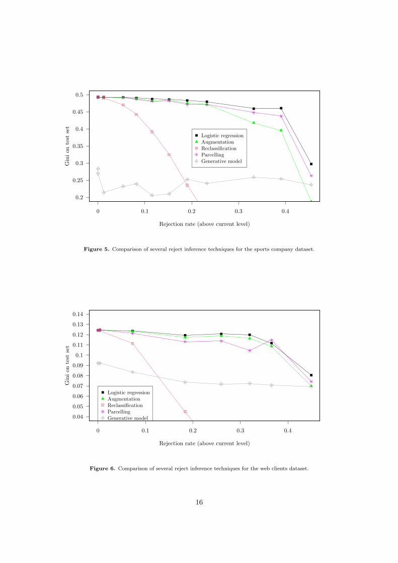
Fuzzy Augmentation and Twins had the exact same performance as logisticregression on financed clients, as shown in Section 3, that is why they wereexcluded from the analysis that follows. Results are displayed on Figures 4, 5 and6. All logistic regression-based models start at the same Gini because for the firstpoint, there are no rejected applicants. Graphically, it seems that all modelsproduce very similar results for a low cut-o↵ value (left side of the plot) and getbad as soon as it is high. Figures have been voluntarily stopped at approximately50% acceptance rate due to computational problems: not enough bad clients left inlearning set, some categorical features’ values not observed anymore in thelearning set but present in the test set, etc.

The generative approach (a multinomial model here) is not quite as good aslogistic regression for low cut-o↵ values most probably for two reasons: first, itmakes more assumptions (on p(x) - see [17]) which leads to a greater modellingmisspecification; second, the features which were selected were engineeredspecifically for logistic regression. Nevertheless, its ability to natively use theunlabeled information showed promising results for large cut-o↵ values.

To conclude, Figures 4, 5 and 6 show that no method works significantly anduniformly better than logistic regression on financed clients on all three portfolios.

In previous works, such experiments (often on a single portfolio and a singledata point, i.e. a single rejection rate) led researchers to conclude positively ornegatively on the benefit of reject inference methods. However, given ourtheoretical findings in Section 3, the fact that in our experiments the results seemhighly dependent on the data and/or the proportion of financed clients, the factthat the performance di↵erences were not statistically significant, we shall

15


Ginion

test

set

0 0.1 0.2 0.3 0.4

0.2

0.25

0.3

0.35

0.4

0.45

0.5


Figure 5. Comparison of several reject inference techniques for the sports company dataset.


Ginion

test

set

0 0.1 0.2 0.3 0.4

0.04

0.05

0.06

0.07

0.08

0.09

0.1

0.11

0.12

0.13

0.14


Figure 6. Comparison of several reject inference techniques for the web clients dataset.

16

conclude that reject inference provides no scope for improving the currentscorecard construction methodology with logistic regression.

5. Discussion: choosing the right model

5.1. Sticking with the financed clients model

Constructing scorecards by using a logistic regression on financed clients is atrade-o↵: on the one hand, it is implicitly assumed that it is well-specified, andthat the missingness mechanism governing the observation of y is MAR andignorable. In other words, we suppose p(y|x) = p✓?(y|x, f). On the other hand,these assumptions, which seem strong at first hand, cannot really be relaxed: first,the use of logistic regression is a requirement from the financial institution.

Second, the comparison of models cannot be performed using standardtechniques since ynf is missing (Section 2.5). Third, strategies 4 (Augmentation)and 6 (Parcelling) which tackle the misspecified model and MNAR settingsrespectively require additional estimation procedures that, supplemental to theirestimation bias and variance, take time from the practitioner’s perspective and arerather subjective (see Sections 3.5 and 3.7), which is not ideal in the bankingindustry since there are auditing processes and model validation teams that mightquestion these practices.

5.2. MCAR through a Control Group

Another simple solution would be to keep a small portion of the population whereapplicants are not filtered: everyone gets accepted, thus creating a true test set asadvocated for in Section 2.5.

Although theoretically perfect, this solution faces a major drawback: it is costly,as many more loans will default. To construct the scorecard, a lot of data isrequired, so the minimum size of the Control Group leads to a much bigger lossthan the amount a bank would accept to lose to get a few more Gini points.

5.3. Keep several models in production: “champion challengers”

Several scorecards could also be developed, e.g. one using each reject inferencetechnique. Each application is randomly scored by one of these scorecards. As timegoes by, we would be able to put more weight on the most performing scorecard(s)and progressively less on the least performing one(s): this is the field ofReinforcement Learning (see [22] for a thorough introduction).

The major drawback of this method, although its cost is very limited unlike theControl Group, is that it is very time-consuming for the credit modeller who has todevelop several scorecards, for the IT who has to put them all into production, forthe auditing process and for the regulatory institutions.

6. Concluding remarks

For years, the necessity of reject inference at CACF and other institutions (as itseems from the large literature coverage this research area has had) has been aquestion of personal belief. Moreover, there even exists contradictory findings inthis area.

By formalizing the reject inference problem in Section 2, we were able topinpoint in which cases the current scorecard construction methodology, using onlyfinanced clients’ data, could be unsatisfactory: under a MNAR missingnessmechanism and/or a misspecified model. We also defined criteria to reinterpretexisting reject inference methods and assess their performance in Section 2.5. Weconcluded that no current reject inference method could enhance the currentscorecard construction methodology: only the Augmentation method (Strategy 4)and the Parcelling method (Strategy 6) had theoretical justifications but introduce

17

other estimation procedures. Additionally, they cannot be compared throughclassical model selection tools (Section 2.5).

We confirmed numerically these findings: given a true model and the MARassumption, no logistic regression-based reject inference method performed betterthan the current method. In the misspecified model case, the Augmentationmethod seemed promising but it introduces a model that also comes with its biasand variance resulting in very close performances compared with the currentmethod. With real data provided by CACF, we showed that all methods gave verysimilar results: the “best” method (by the Gini) was highly dependent on the dataand/or the proportion of unlabelled observations. Last but not least, in practicesuch a benchmark would not be tractable as ynf is missing, thus making it alsohighly dependent on the way we simulate not-financed clients from previouslyfinanced clients. In light of those limitations, adding to the fact that implementingthose methods is a non-negligible time-consuming task, we recommend creditmodellers to work only with financed loans’ data unless there is significantinformation available on either rejected applicants (ynf - credit bureau informationfor example, which does not apply to France) or on the acceptance mechanism �in the MNAR setting. On a side note, it must be emphasized that this work onlyapplies to logistic regression but can be extended to all “local” models per theterminology introduced in [27]. For “global” models, explicitly or implicitlyobtaining their predictive model p✓(y|x) as a by-product of modelling p(x) orp(x|y), e.g. decision trees, it can be shown that they are biased even in the MARand well-specified settings, thus requiring ad hoc reject inference techniques suchas an adaptation of the Augmentation method (Strategy 4).

All experiments (except on real data) can be reproduced by using the Rpackage scoringTools (see [7] and Appendix B).

References

[1] B. Anderson, Using Bayesian networks to perform reject inference, Expert Systems withApplications 137 (2019), pp. 349–356.

[2] J. Banasik and J. Crook, Reject inference, augmentation, and sample selection, EuropeanJournal of Operational Research 183 (2007), pp. 1582–1594. Available at http://www.sciencedirect.com/science/article/pii/S0377221706011969.

[3] G. Celeux and G. Govaert, A classification em algorithm for clustering and two stochasticversions, Computational statistics & Data analysis 14 (1992), pp. 315–332.

[4] O. Chapelle, B. Schlkopf, and A. Zien, Semi-Supervised Learning, 1st ed., The MIT Press,2010.

[5] A.P. Dempster, N.M. Laird, and D.B. Rubin, Maximum likelihood from incomplete datavia the em algorithm, Journal of the royal statistical society. Series B (methodological)(1977), pp. 1–38.

[6] B. Efron, The e�ciency of logistic regression compared to normal discriminant analysis,Journal of the American Statistical Association 70 (1975), pp. 892–898.

[7] A. Ehrhardt, Credit Scoring Tools: the scoringTools package (2020). Availableat https://CRAN.R-project.org/package=scoringTools, https://adimajo.github.io/scoringTools.

[8] A. Feelders, Credit scoring and reject inference with mixture models, International Jour-nal of Intelligent Systems in Accounting, Finance & Management 9 (2000), pp. 1–8. Available at http://www.ingentaconnect.com/content/jws/isaf/2000/00000009/00000001/art00177.

[9] A. Guizani, B. Souissi, S.B. Ammou, and G. Saporta, Une comparaison de quatre tech-niques d’inference des refuses dans le processus d’octroi de credit, in 45 emes Journeesde statistique. 2013. Available at http://cedric.cnam.fr/fichiers/art_2753.pdf.

[10] Y. Kang, R. Cui, J. Deng, and N. Jia, A novel credit scoring framework for auto loan usingan imbalanced-learning-based reject inference, in 2019 IEEE Conference on ComputationalIntelligence for Financial Engineering & Economics (CIFEr). IEEE, 2019, pp. 1–8.

[11] N.M. Kiefer and C.E. Larson, Specification and informational issues in credit scoring,

18

Available at SSRN 956628 (2006). Available at http://papers.ssrn.com/sol3/papers.cfm?abstract_id=956628.

[12] N. Kozodoi, P. Katsas, S. Lessmann, L. Moreira-Matias, and K. Papakonstantinou, Shal-low Self-Learning for Reject Inference in Credit Scoring, in Joint European Conference onMachine Learning and Knowledge Discovery in Databases. Springer, 2019, pp. 516–532.

[13] R. Lebret, S. Iovle↵, F. Langrognet, C. Biernacki, G. Celeux, and G. Govaert, Rmixmod:the r package of the model-based unsupervised, supervised and semi-supervised classifica-tion mixmod library, Journal of Statistical Software (2015), pp. In–press.

[14] Z. Li, Y. Tian, K. Li, F. Zhou, and W. Yang, Reject inference in credit scoring usingsemi-supervised support vector machines, Expert Systems with Applications 74 (2017),pp. 105–114.

[15] R.J. Little and D.B. Rubin, Statistical analysis with missing data, John Wiley & Sons,2014.

[16] R.A. Mancisidor, M. Kamp↵meyer, K. Aas, and R. Jenssen, Deep generative models forreject inference in credit scoring, Knowledge-Based Systems (2020), p. 105758.

[17] G. McLachlan and D. Peel, Finite mixture models, John Wiley & Sons, 2004.[18] G. Molenberghs, C. Beunckens, C. Sotto, and M.G. Kenward, Every missingness not at

random model has a missingness at random counterpart with equal fit, Journal of theRoyal Statistical Society: Series B (Statistical Methodology) 7 (2008), pp. 371–388.

[19] H.T. Nguyen, Reject inference in application scorecards: evidence from France, Tech. Rep.,University of Paris West-Nanterre la Defense, EconomiX, 2016. Available at http://economix.fr/pdf/dt/2016/WP_EcoX_2016-10.pdf.

[20] T.J. O’neill, The general distribution of the error rate of a classification procedure withapplication to logistic regression discrimination, Journal of the American Statistical As-sociation 75 (1980), pp. 154–160.

[21] F. Shen, X. Zhao, and G. Kou, Three-stage reject inference learning framework for creditscoring using unsupervised transfer learning and three-way decision theory, Decision Sup-port Systems 137 (2020), p. 113366.

[22] R.S. Sutton and A.G. Barto, Reinforcement Learning: An Introduction, 2nd ed., The MITPress, 2018, Available at http://incompleteideas.net/book/the-book-2nd.html.

[23] V. Vandewalle, Estimation et selection en classification semi-supervisee, Theses, Uni-versite des Sciences et Technologie de Lille - Lille I, 2009. Available at https://tel.archives-ouvertes.fr/tel-00447141.

[24] E. Viennet, F.F. Soulie, and B. Rognier, Evaluation de techniques de traitement des refusespour l’octroi de credit, arXiv preprint cs/0607048 (2006). Available at http://arxiv.org/abs/cs/0607048.

[25] H. White, Maximum likelihood estimation of misspecified models, Econometrica 50 (1982),pp. 1–25. Available at http://www.jstor.org/stable/1912526.

[26] Y. Xia, X. Yang, and Y. Zhang, A rejection inference technique based on contrastivepessimistic likelihood estimation for p2p lending, Electronic Commerce Research and Ap-plications 30 (2018), pp. 111–124.

[27] B. Zadrozny, Learning and evaluating classifiers under sample selection bias, in Proceed-ings of the twenty-first international conference on Machine learning. ACM, 2004, p. 114.

AppendicesAppendix A. Missingness mechanism: definitions

When Z = nf, Y is not observed. In presence of covariates X, there are threeclassical situations regarding p(x, y, z) first investigated in [15], worth discussing inCredit Scoring : MCAR, MAR and MNAR.

19

A.1. Missing Completely At Random (MCAR)

The financing mechanism Z is considered independent of the covariates X and therepayment Y (given the covariates X), s.t.:

8x, y, z, p(z|x, y) = p(z).

A.2. Missing At Random (MAR)

The financing mechanism Z is considered independent of the repayment Y , s.t.:

8x, y, z, p(z|x, y) = p(z|x).

Most importantly for Credit Scoring applications, this is equivalent to:

8x, y, z, p(y|x, z) = p(y|x).

A.3. Missing Not At Random (MNAR)

This is the most general case where:

9x, y, p(z|x, y) 6= p(z|x).

In other words, financing depends on the creditworthiness of the client evenafter taking into account covariates X. In particular, this impliesp(y|x, nf) 6= p(y|x, f), which is implicitly assumed by most Credit Scoringpractitioners when they refer to reject inference.

A.4. Ignorability

Complementary to the stochastic dependencies between X, Y and Z, there is afunctional dependence between p(z|x, y) and p(y|x) when modelled through thegeneral parametric family p�(y, z|x) as in Equation (1), i.e. in general, � 6= (�,✓).In other words, in the MAR ignorable case, we have � = (�,✓) such that thelog-likelihood `(�; T ) consists in two independent terms depending respectively on✓ and � (Equation (5)). Since we are only interested in p(y|x), we can safely“ignore” p�(z|x) and maximize the quantity of interest: `(✓; Tf).

Appendix B. Computational considerations

Logistic regression is fitted using the R function glm which estimates logisticregression parameters by a Newton-Raphson algorithm similar to the onesimplemented in SAS (proc logistic), classically used in credit scoring. Generativemodels use Gaussian mixtures for continuous features and multinomial models forcategorical data. To benefit from their native use of unlabeled information thanksto the EM-algorithm as introduced in Section 2.3, we used the Rmixmod package(see [13]).

Additionally, reject inference methods were coded in the R packagescoringTools (see [7]) which can be found on CRAN. Installation instructions,additional remarks, and access to the scripts used to generate the plots of thisarticle are given on https://adimajo.github.io/scoringTools.

In particular, typing vignette(‘scoringTools’), vignette(‘figure1’),vignette(‘figure2’), vignette(‘figure3’),

20

vignette(‘appendix tree biasedness’) will respectively present the code usedfor how to use the package and Figures 1, 2, 3, and a similar example with adecision tree which, contrary to logistic regression (to some extent) becomes “morebiased” as the number of simulated reject applicants grows.

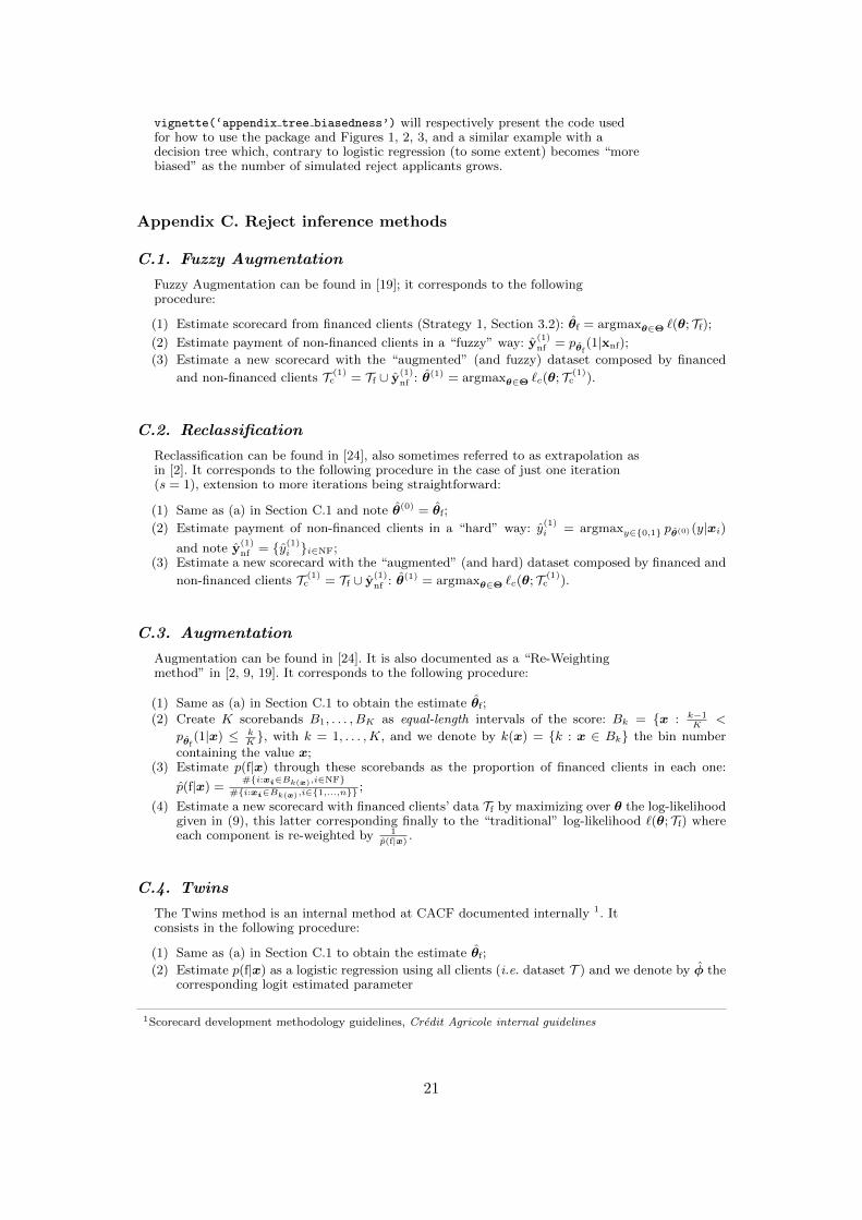
Appendix C. Reject inference methods

C.1. Fuzzy Augmentation

Fuzzy Augmentation can be found in [19]; it corresponds to the followingprocedure:

(1) Estimate scorecard from financed clients (Strategy 1, Section 3.2): ✓f = argmax✓2⇥ `(✓; Tf);

(2) Estimate payment of non-financed clients in a “fuzzy” way: y(1)nf = p✓f

(1|xnf);(3) Estimate a new scorecard with the “augmented” (and fuzzy) dataset composed by financed

and non-financed clients T (1)c = Tf [ y(1)

nf : ✓(1) = argmax✓2⇥ `c(✓; T (1)

c ).

C.2. Reclassification

Reclassification can be found in [24], also sometimes referred to as extrapolation asin [2]. It corresponds to the following procedure in the case of just one iteration(s = 1), extension to more iterations being straightforward:

(1) Same as (a) in Section C.1 and note ✓(0) = ✓f;

(2) Estimate payment of non-financed clients in a “hard” way: y(1)i = argmaxy2{0,1} p✓(0)(y|xi)

and note y(1)nf = {y(1)

i }i2NF;(3) Estimate a new scorecard with the “augmented” (and hard) dataset composed by financed and

non-financed clients T (1)c = Tf [ y(1)

nf : ✓(1) = argmax✓2⇥ `c(✓; T (1)

c ).

C.3. Augmentation

Augmentation can be found in [24]. It is also documented as a “Re-Weightingmethod” in [2, 9, 19]. It corresponds to the following procedure:

(1) Same as (a) in Section C.1 to obtain the estimate ✓f;(2) Create K scorebands B1, . . . , BK as equal-length intervals of the score: Bk = {x : k�1

K <p✓f

(1|x) kK }, with k = 1, . . . ,K, and we denote by k(x) = {k : x 2 Bk} the bin number

containing the value x;(3) Estimate p(f|x) through these scorebands as the proportion of financed clients in each one:

p(f|x) = #{i:xi2Bk(x),i2NF}#{i:xi2Bk(x),i2{1,...,n}} ;

(4) Estimate a new scorecard with financed clients’ data Tf by maximizing over ✓ the log-likelihoodgiven in (9), this latter corresponding finally to the “traditional” log-likelihood `(✓; Tf) whereeach component is re-weighted by 1

p(f|x) .

C.4. Twins

The Twins method is an internal method at CACF documented internally 1. Itconsists in the following procedure:

(1) Same as (a) in Section C.1 to obtain the estimate ✓f;(2) Estimate p(f|x) as a logistic regression using all clients (i.e. dataset T ) and we denote by � the

corresponding logit estimated parameter

1Scorecard development methodology guidelines, Credit Agricole internal guidelines

21

(3) Estimate a new scorecard with financed clients’ data merging two novel covariates, namely(1,xf)

0✓f and (1,xf)0�, thus it consists in maximizing over ✓ the following log-likelihood:

`(✓; (1,xf)0✓f, (1,xf)

0�f,yf) =X

i2F

ln(p✓(yi|(1,xi)0✓f, (1,xi)

0�)), (C1)

providing an estimated denoted by ✓twins;(4) Estimate now the final scorecard, this time by using the Fuzzy Augmentation method where

✓f is replaced by ✓twins at Step (a).

C.5. Parcelling

Parcelling is a process of reweighing according to the probability of default byscore-band that is adjusted by the credit modeler. It has been documented in[2, 9, 24], as well as an internal document of CACF 1. It corresponds to thefollowing steps:

(1) Same as (a) in Section C.1 to obtain the estimate ✓f;(2) Same as (b) in Section C.3 to create K scorebands B1, . . . , BK ;

(3) Estimate payment of non-financed clients in a “fuzzy” way: y(1)i = 1 � ✏k(xi)p✓f

(0|xi, f), for

i 2 NF, and then note y(1)nf = {y(1)

i }i2NF;(4) Estimate a new scorecard by Step (c) of the Fuzzy Augmentation method in Section C.1.

22

Reject Inference Methods in Credit Scoring: A rational review

Documents

Transcript of Reject Inference Methods in Credit Scoring: A rational review