Regulating Conglomerates: Evidence from anEnergy Conservation Program in China∗

Qiaoyi Chen Zhao Chen Zhikuo LiuFudan University Fudan University Fudan University

Juan Carlos Suarez Serrato Daniel Yi XuDuke University Duke University

& NBER & NBER

July 15, 2021

Abstract

We study a prominent energy regulation affecting large Chinese manufacturers that arepart of broader conglomerates. Using detailed firm-level data and difference-in-differencesresearch designs, we show that regulated firms cut output and shifted production to unreg-ulated firms in the same conglomerate instead of improving their energy efficiency. Con-glomerate spillovers account for 40% of the output loss of regulated firms and substantiallyreduce aggregate energy savings. Using a structural model, we show that alternative po-lices that use public information on business networks could lower the shadow cost of theregulation by more than 40% and increase aggregate energy savings by 10%.JEL Codes: Q48, L51, O44, H23.

∗We are very grateful for discussions from Stefan Lamp, Mar Reguant, Nick Ryan, and Shaoda Wang andfor comments from Hunt Allcott, Soren Anderson, Prabhat Barnwal, Raj Chetty, Julie Cullen, David Cutler,Michael Davidson, Michael Dinerstein, Matt Gentzkow, Ed Glaeser, Ken Gillingham, Josh Gottlieb, MichaelGreenstone, Caroline Hoxby, Kelly Jones, Matthew Kahn, Louis Kaplow, Lawrence Katz, Stephanie Kestelman,Justin Kirkpatrick, Thibaut Lamadon, Ashley Langer, Shanjun Li, Neale Mahoney, Justin Marion, Leslie Martin,Magne Mogstad, Ben Olken, Edson Severnini, Joe Shapiro, Felix Soliman, Michael Song, Stefanie Stantcheva,Chris Timmins, Reed Walker, Heidi Williams, Xiaodong Zhu, and seminar participants at American University,ASSA, Barcelona Summer Forum, Cowles Foundation Summer Conference, Fudan University, FRB of Atlanta,Harvard, Helsinki GSE, Michigan State University, NBER Public, NBER China, Paris School of Economics,Peking University, SHUFE, Stanford University, University of Chicago, University of Toronto, UCSC, UCSD,University du Quebec a Montreal, University of Oxford, University of Michigan, and the 9th Mannheim Conferenceon Energy and the Environment. We thank IntSig Information for providing China’s Administrative RegistrationData (CARD). All errors remain our own.

Balancing economic growth with the negative side effects of industrialization—such as carbon

emissions and pollution—is a central problem of governments in emerging economies. Nowhere

is this problem more important or consequential than in China. As Figure 1 shows, energy

regulation is of national and global importance given that the industrial energy use of China

overshadowed that of other leading economies in the early years of the 21st century.

This paper studies the effects of a large program aimed at curbing the energy use of Chinese

industrial firms. The regulation that we study—the “Top 1,000” program—targeted the largest

energy-consuming firms in the most energy-intensive industries. The regulation was designed

following examples of “voluntary agreement” programs in developed countries that relied on the

belief that firms could significantly reduce their energy use by improving their energy efficiency.

The implementation of the program was adjusted to Chinese institutions and constraints, with

the result that in practice, lowering energy consumption became the main regulatory objective.

Understanding the effects of this regulation is central to broader questions of energy conservation

in China. This is both because the firms regulated by this program accounted for 47% of total

industrial energy use in China in 2004 and because the perceived success of the regulation led

the government to significantly expand the program in later years.

This paper asks four questions that characterize the effectiveness of the Top 1,000 program.

Importantly, these questions account for the fact that, as in several developing countries, in-

dustrial firms in China are often part of much larger business networks.1 First, how does the

regulation impact the production and energy use of regulated firms and firms that are related

through ownership networks? Second, what are the distortionary effects of the regulation and

how does the ability to shift production within a conglomerate lower the cost of the program

for regulated firms? Third, how do conglomerate and market spillovers alter the effects of the

policy on industrial energy use and welfare? Finally, can the government use information on

conglomerate networks to improve energy regulation?

We answer these questions by combining difference-in-differences research designs with an

industry equilibrium model featuring conglomerate production. First, using a difference-in-

differences strategy, we estimate that regulated firms reduced their energy use by 12%–16%.

Regulated firms achieved these reductions by lowering output; we find no impact on their energy

efficiency. Second, we use detailed data on business networks to study whether conglomerates

reallocated production across related firms. Using a second difference-in-differences design, we

find that unregulated firms in the same conglomerate as regulated firms increased both output

and energy use. This result uncovers an important margin of adjustment that allowed Chinese

conglomerates to shift 40% of the output decline in regulated firms to unregulated affiliates.

1Ramachandran et al. (2013) describe the growing importance of conglomerates in India, China, and LatinAmerica.

1

Third, we specify and estimate a model of conglomerate production that matches our setting

and the estimated impacts of the policy. We quantify that the ability of conglomerates to shift

production lowered the shadow cost of the regulation from 11.2% of input costs to 8.7%. We also

evaluate the welfare effects of the program and quantify that the Top 1,000 program improves

welfare when the social cost of carbon exceeds $160.2 Finally, we show that the government can

use public information on conglomerate networks to design a conglomerate-level regulation that

would increase energy savings by 10% for the same welfare cost.

Overall, we find that while the regulation reduced the energy consumption of large firms,

the promise of achieving these savings through improved energy efficiency failed to materialize.

Instead, regulated firms reduced their energy use by decreasing their output and by reallocating

part of the lost economic activity across business networks, which significantly lowered the pol-

icy’s impact on energy reduction. While the ability to shift production lowered the shadow cost

for regulated conglomerates, the Top 1,000 program distorted the within-conglomerate allocation

of production. The government can alleviate this distortion by using publicly available data on

business networks to improve the design of energy regulation.

We develop these results in three steps. First, we implement a difference-in-differences strat-

egy using firms in similar industries that were regulated in later years as controls. We use an

event-study specification to show that Top 1,000 firms and unregulated firms had similar trends

prior to the regulation. We estimate that regulated firms reduced their energy use by about

12%–16%. These estimates are robust to inclusion of industry-by-year and province-by-year

fixed effects and of controls for firm characteristics. Since the regulated firms consumed 670

million tons of coal equivalent (tce) in 2004, taking these results at face value would imply a

direct reduction in energy use amounting to close to 100 million tce annually. However, we also

document that these firms saw a decline in output of between 10% and 23%, and we do not find

meaningful or statistically significant changes in energy efficiency. The lack of gains in energy

efficiency suggest two hypotheses. The first is that firms had limited potential to increase energy

efficiency from a technological perspective—i.e., that there was no “low-hanging fruit” (e.g., All-

cott and Greenstone, 2012). A second hypothesis is that firms were able to escape the regulatory

burden by shifting production to related parties.

Our second set of analyses leverages detailed business registration data to map the conglom-

erate networks of regulated firms. If regulated firms were able to escape the regulation by shifting

production to related parties, we would expect to see an increase in both the output and energy

use of firms linked to regulated firms through ownership networks. We test this hypothesis using

2The Top 1,000 program had the stated goal of reducing industrial energy use to lower emissions that con-tribute to global warming. While energy use reductions also lower local pollution, pollution reduction was not astated goal of the program (Price et al., 2010). Our welfare analyses evaluate the program’s objective to reduceaggregate energy use.

2

a difference-in-differences strategy that compares unregulated but related firms to unregulated

and unrelated firms. To ensure that these two groups of firms are similar, we use a matching

procedure based on pre-regulation characteristics to find a suitable set of control firms. These

analyses show that after the reform, regulated conglomerates shifted production to affiliates that

were not subject to the regulation. Specifically, we find an increase in firm output of 13% and

similar increases in other measures such as profits, sales, capital, labor, and energy use.3 Impor-

tantly, we find increases in the economic activity of related firms only when their line of business

coincides with the narrowly defined (4-digit) industry classification of the regulated firm. As a

placebo test, we show that related firms in other industries did not see an increase in economic

activity. Because related firms are smaller than regulated firms, we calculate that conglomerates

were able to shift 40% of the output decline in regulated firms to related parties. We corroborate

the finding that conglomerates were not able to fully shift the production decline in Top 1,000

firms to affiliates by showing that unregulated and unrelated firms also increase output as a

result of the regulation. These results show that a complete assessment of the effects of the Top

1,000 program must take into account both within-conglomerate and market-level leakage.

Our last set of analyses use an industry equilibrium model of conglomerate production that

accounts for within-conglomerate spillovers to related firms as well as for market spillovers. The

model clarifies the interpretation of our difference-in-differences estimates, computes the shadow

cost of the regulation at the conglomerate level, and quantifies the aggregate and welfare effects

of the Top 1,000 program. We estimate the model parameters by matching moments of the

firm size distribution and patterns of within-conglomerate allocation of production prior to the

regulation. We then use our reduced-form estimates as out-of-sample validations of the model,

which show that our estimated model is able to replicate the estimated effects of the policy.

Our estimated model quantifies the shadow cost of the Top 1,000 program at 8.7% of input

costs. The ability of conglomerates to shift production across related firms decreased the shadow

cost of the program. The shadow cost of the program would have been 11.2% in a hypothetical

case where the government prevented conglomerate-level leakage. The shadow cost of the pro-

gram would have been 40% smaller had the government instead regulated the total energy use

of the conglomerate.

We then use the model to quantify the aggregate and welfare effects of the Top 1,000 pro-

gram. Accounting for market and conglomerate leakage, we calculate that the program reduced

aggregate energy use by 4%, an annual decrease of about 48 million tce. A calibration of the

social cost of energy-related emissions shows that the program raises welfare as long as the social

cost of carbon exceeds $160 per ton of carbon. Using the model, we show that expanding the

3In Appendix C we show that the program did not significantly shift production to more polluted or populatedareas. For this reason, our model and welfare analyses abstract from spatial implications of the policy.

3

program by increasing the number of regulated firms or by tightening energy saving targets leads

to similar trade-offs. A government facing administrative constraints would thus prefer to tighten

the stringency of the regulation rather than increase the number of regulated firms.

The model allows us to compare the aggregate and welfare effects of incomplete regulations,

such as the Top 1,000 program, to policies that would be preferable absent political or administra-

tive constraints, such as a universal energy tax. First, we show that the government can increase

aggregate energy savings by 10% for the same welfare cost by leveraging publicly available data

on the ownership networks of regulated conglomerates. By targeting conglomerates instead of

firms, such a regulation would avoid distorting the within-conglomerate allocation of production.

Second, the model shows that a conglomerate-level regulation closely approximates the effects of

a size-dependent energy tax that applies to all affiliates in conglomerates with Top 1,000 firms.

Finally, we find that this size-dependent tax is only slightly inferior to a universal energy tax.

These results highlight the promise of using information on the conglomerate networks of large

Chinese manufacturers to improve the design of energy regulations.

Finally, we show that our model results are robust to using a wide range of alternative model

specifications and parameter values. First, we extend the model to consider the possibility that

firms responded to the regulating by improving their energy efficiency. Consistent with our

empirical results, we find that firms faced significant costs of improving their energy efficiency.

Second, we extend the model to allow for preexisting differences in energy efficiency between

regulated and unregulated firms. Finally, we show that our results are robust to alternative as-

sumptions of parameter values and model specifications. Across these wide-ranging assumptions,

we estimate that the SCC that rationalizes the policy is between $112 and $196.

This paper contributes to our understanding of whether energy regulations and interventions

aimed at improving energy efficiency are effective in developing countries (e.g., Duflo et al., 2013,

2018; Greenstone and Jack, 2015; Ryan, 2018; Ito and Zhang, 2020).4 In the Chinese context,

the government’s use of high-powered incentives that tie environmental performance to cadre

promotion has been shown to provide a strong mechanism to enforce environmental policies

(Kahn et al., 2015; Jia, 2017; He et al., 2020). In their discussion of recent efforts to curb energy

use in China, Auffhammer and Gong (2015) note that the Top 1,000 program along with its

expanded version in later years are the “most significant national programs” focusing on energy

efficiency and energy conservation. Using industry-level data, Ke et al. (2012) argue that the

4See Gillingham et al. (2018) for a review of this literature in the context of developed countries. While thisliterature mostly focuses on non-industrial energy use, some of the rationales explaining the under-investmentin energy efficiency—such as imperfect information or behavioral biases—may also apply to firms. For instance,Anderson and Newell (2004) show that, while some US firms adopt energy conservation projects in response toenergy audits, economic considerations play an important role in explaining why not all firms adopt these projects.In our setting, the ability of firms to escape the burden of the regulation by shifting production to related firmsadds to the potential explanations for under-investment in energy efficiency.

4

Top 1,000 program led to significant declines in the energy intensity of regulated sectors. By

using detailed firm-level data and tracing the effects of the regulation along business ownership

networks, our results provide a fundamental reassessment of the effectiveness of the Top 1,000

program.

The result that the Top 1,000 program impacted economic activity in regulated and unreg-

ulated firms contributes to the literature studying the economic costs of environmental regula-

tions. In the US, researchers have documented significant effects of environmental regulations on

emissions and economic activity (e.g., Greenstone, 2002; Greenstone et al., 2012; Walker, 2013;

Shapiro and Walker, 2018; Curtis, 2018). Colmer et al. (2020) find that French firms that are

subject to the European Union’s emissions trading scheme do not experience significant declines

in production and that their declines in energy do not spill over to unregulated firms. He et

al. (2020) show that Chinese firms that face more stringent regulations experience significant

decreases in productivity. Our paper contributes to our understanding of the economic cost of

energy regulation in China, which consumes the lion’s share of global industrial energy.

Researchers have also documented that regulations can have spillover effects along firm net-

works. For instance, Hanna (2010) finds that multinational firms respond to domestic environ-

mental regulations by increasing their investment in foreign countries, and Gibson (2019) and

Soliman (2020) find that firms may also shift economic activity to unregulated plants in counties

that are subject to less stringent regulations. Conglomerate spillovers are particularly important

in our setting since the Top 1,000 program targeted very large firms with elaborate ownership

networks. Our detailed business registration data provide a unique view into how this regulation

affected the production decisions of large Chinese conglomerates and how conglomerate spillovers

impacted the effectiveness of the regulation. Our model leverages these spillovers to quantify the

marginal cost of the regulation, using the fact that conglomerates incur a loss when they distort

the within-conglomerate allocation of production (see, e.g., Anderson and Sallee, 2011).

Our paper also takes into account the roles of leakage and market competition in environmen-

tal regulation. Research has shown that emissions leakage to unregulated firms can significantly

alter the effects and design of environmental policies (e.g., Fowlie, 2009; Holland, 2012; Fischer

and Fox, 2012; Bushnell et al., 2014; Baylis et al., 2014; Fowlie and Reguant, 2021). We abstract

from strategic interactions between firms in a setting with monopolistic competition since we

study manufacturing industries with a large number of firms that compete in national markets.5

This paper quantifies the aggregate and welfare effects of the Top 1,000 program by combining

microdata on the operations of Chinese industrial firms, transparent research designs that iden-

tify direct and spillover effects of a prominent energy regulation, and an industry equilibrium

5Studies of energy regulation with strategic interaction often focus on concentrated industries (see, e.g.,Mansur, 2007; Ryan, 2012; Fowlie et al., 2016).

5

model that is consistent with the estimated effects of the program. The combination of these

approaches accounts for market competition and leakage effects and shows that conglomerate

spillovers are a distinct force that plays a quantitatively important role in the context of China

and that feasible conglomerate-level regulations can improve the regulation of energy.

This paper is organized as follows. Section 1 describes the policy context and the data that we

use to measure firm responses to the regulation and the ownership networks of regulated firms.

Section 2 estimates direct effects of the Top 1,000 program on regulated firms, and Section 3

estimates indirect effects on unregulated firms that belong to the business networks of regulated

firms. Section 4 describes our model of conglomerate regulation, and Section 5 estimates the

model parameters. Section 6 uses the model to quantify the shadow cost of the policy and to

analyze the aggregate and welfare effects of the regulation. Section 7 explores extensions of the

model, and Section 8 concludes.

1 Policy Background and Data

This section describes the Top 1,000 energy savings program. We also describe the different

datasets that we use to measure economic activity and energy use as well as our strategy to map

the ownership networks of Chinese conglomerates.

1.1 The Top 1,000 Program

To save energy and reduce related carbon emissions, the Chinese government’s 11th Five-Year

Plan (11FYP) set an ambitious goal of reducing the country’s energy intensity—defined as energy

consumption per unit of GDP—by 20% between 2006 and 2011 (Price et al., 2010). Since

the industrial sector accounts for 70% of total energy consumption, the government designed

policies that focused on nine energy-intensive industries, which accounted for 80% of the country’s

industrial energy use. One of these key initiatives was the Top 1,000 Energy Saving Program,

which targeted the firms with the highest energy consumption in the most energy-intensive

industries.

The Top 1,000 program was first announced by the National Development and Reform Com-

mission in April 2006, and the corresponding monitoring and assessment measures were released

in 2007. The name “Top 1,000” refers to the 1, 008 industrial firms in the nine energy-intensive in-

dustries with energy consumption above 180 thousand tce in 2004. The total energy consumption

of these 1,008 super-firms was 670 million tce in 2004, accounting for 47% of China’s industrial

energy consumption and 33% of its total energy consumption. Importantly, since the policy was

announced in 2006 and selected firms based on their retrospective 2004 energy consumption,

it was not possible to manipulate the list of program participants. Moreover, the list of firms

6

regulated by the program did not change during the five-year period. Table 1 reports the number

of firms and their share of energy consumption in each of the regulated industries. Among Top

1,000 firms, those in the iron and steel, chemical, and electric power industries accounted for

around 63% of the firms and 68% of the regulated energy consumption in 2005.

The Top 1,000 program was designed based on the belief that Chinese industries could sig-

nificantly increase energy efficiency at a low cost (e.g., McKinsey & Co., 2009). The program

was influenced by voluntary agreement programs in developed countries and had two stated

goals: to significantly increase the energy efficiency of these super-firms and to save 100 million

tce in energy consumption by 2011. Given the program’s quick implementation, many aspects

of voluntary agreement programs (such as providing technological expertise or financing energy

efficiency improvements) played a relatively minor role (Price et al., 2010). In practice, firms

were regulated based on energy use only and not on energy efficiency.

To implement the policy, the central government assigned a target reduction in energy use to

each provincial government. In turn, local officials assigned individual quotas to each of the Top

1,000 firms. These firms were subject to annual energy audits carried out by a third party and

also faced potential additional audits from the Ministry of Industry and Information Technology

and the National Energy Administration. Leaders of provincial governments and state-owned

enterprises were then evaluated on whether these energy saving targets were met. As a result,

local government officials monitored and enforced the energy saving targets of Top 1,000 firms

very closely.6 The effect of this strict supervision is evident in Table A.1, where we report the

results of the government’s annual assessment. This table shows a very high compliance rate. In

fact, the total energy saving target was achieved in 2008, two years ahead of schedule. At the

end of the 11FYP, the government estimated energy savings of 165.49 million tce, far beyond

the original target of 100 million tons.7

Due to this perceived success under the 11FYP, the Top 1,000 program was expanded into

the “Top 10,000” Energy Savings Program during the 12th Five-Year Plan (12FYP) in 2012. In

this case, “Top 10,000” refers to 16,078 energy-intensive firms with energy consumption above

10 thousand tce in 2010. These firms account for 60% of China’s total energy consumption. As

in the Top 1,000 program, firms among the Top 10,000 were required to improve their energy

efficiency with a goal of saving a total of 250 million tce during the 12FYP. Our primary analysis

6Under the “one-vote veto” criteria, officials would not be considered for promotions or awards if the provinceor any of the local Top 1,000 firms did not achieve their targets. Similarly, the leaders of state-owned enterprisesthat did not meet the target did not receive annual bonuses. In interviews with executives of Top 1,000 firms,we confirmed that local officials had the power to stop production at regulated firms if the firm did not meet itsenergy target. In this way, the Chinese setting contrasts with other developing country settings where the designof incentives for energy auditors plays a key role (e.g., Duflo et al., 2013, 2018).

7While government estimates of compliance may be subject to misreporting (Karplus et al., 2020), our analysesrely on multiple measures of output and energy use from survey and administrative data that are unrelated tothe government’s evaluation of the program.

7

focuses on Top 1,000 firms between 2001 and 2011. Since the industrial firms in the Top 10,000

(but not in the Top 1,000) were also energy intensive but were not regulated during the 11FYP,

they serve as useful controls for our empirical analysis.8

1.2 Firm Data

Our empirical analyses combine several rich datasets that describe production and energy use at

these firms. The first dataset that we use is the list of firms in the Top 1,000 and Top 10,000

programs from the National Development and Reform Commission. We merge these lists with

the Annual Survey of Industrial Firms (ASIF) from the National Bureau of Statistics (2001–2009

and 2011).9 This dataset provides detailed information on a firm’s industry, address, ownership,

output, and financial information and covers all industrial firms with annual revenue above 5

million RMB (approximately 800,000 USD).

We complement these data with two additional datasets. First, we collect detailed information

on firm energy consumption from 2001 to 2010 from China’s Environmental Statistics Database

(CESD) provided by China’s Ministry of Environmental Protection. The CESD data are subject

to audits by environmental protection agencies at both local and national levels. Second, we

merge data from the Annual Tax Survey (ATS) for 2009 and 2010. One advantage of using

multiple datasets is that we can cross-check our data to ensure our results are not driven by

misreporting or other data quality issues. In Figure A.1, we show that firms report similar

output and coal consumption in the CESD and tax data, which are collected independently and

are not used to evaluate compliance with energy and environmental policies.

Panel A of Table 2 reports summary statistics for the Top 1,000 and Top 10,000 firms in

our sample. This sample includes about 8,700 observations for Top 1,000 firms and 81,000

observations for Top 10,000 firms over a period of 10 years. Our combined datasets therefore

capture the majority of the economic activity in the Top 1,000 and Top 10,000 firms. Because the

CESD reports energy consumption only from primary sources (e.g., coal, oil, gas), our analyses

of energy use and energy efficiency exclude firms in industries that rely mainly on electricity.10

For this reason, the sample of firms with energy consumption data is smaller.

As we show in Panel A of Table 2, Top 1,000 firms are larger, older, more likely to be state

owned, and more export oriented than Top 10,000 firms. This table also shows that Top 1,000

8An important consideration is whether firms that were later part of the Top 10,000 expected that the Top1,000 program would be expanded. This is unlikely to be the case since the details of the program were developedafter the 12FYP by the National Development and Reform Commission, which did not announce the Top 10,000program until 2012.

9Appendix A describes our merged data. As is well known in the literature, data for the 2010 ASIF displaya number of irregularities and are often excluded from statistical analyses. As we show below, our results arerobust to using administrative tax data on production and energy use for 2009 and 2010.

10In practice, we exclude industries where electricity consumption accounts for more than 30% of total energyconsumption. As we show below, our results are robust to setting this threshold to between 15% and 50%.

8

firms are slightly less energy efficient (defined as the ratio of output to energy use) than Top

10,000 firms. However, this difference is driven mostly by industry differences, since Top 1,000

firms are more likely to be in energy-intensive heavy industries. As we show below, our empirical

analyses are robust to controlling for these firm-level characteristics.11

1.3 Mapping Conglomerate Networks

We identify firms’ ownership networks using data from China’s Administrative Registration

Database (CARD). These data are collected by the State Administration of Industry and Com-

merce and list the registration information of all firms in China starting in 1980, including firm

name, registration number, date of establishment, address, ownership, registered capital and re-

lated legal persons. Importantly, the data provide detailed shareholder information, which allows

us to construct firm ownership networks at multiple levels.

We construct ownership networks using the four types of linkages displayed in Figure 2. First,

we include wholly owned subsidiaries of regulated firms as related parties. Second, we include

firms that are at least partially owned by regulated firms. We consider firms to be related if they

are owned by a regulated firm by up to two levels of investment relations. Although in practice

most related firms are fully owned, we require that the regulated firm own at least 25% of the

related firm at each level of investment. Third, we include shareholders of regulated firms, and

we allow up to two levels of shareholder links. Finally, we also include firms that are fully or

partly owned by the shareholders of a regulated firm.12 We exclude firms that are related only

through the state-owned management committee.

Panel B of Table 2 shows that we can identify 46,178 related parties of Top 1,000 firms in

the CARD. Since a large number of related parties are service firms or small firms not recorded

in the ASIF, we match 7,329 firms in the ASIF. In our baseline regressions, we require related

firms to be in the same 4-digit industry as a related Top 1,000 firm. Our main sample of related

firms includes 2,466 industrial firms.13 Since it is likely very hard to shift production to firms in

other narrowly defined industries, we analyze firms within the same 2-digit industry but outside

4-digit industries in a placebo test. A potential concern with CARD data is that some of the

related firms may not be engaged in production and may, in fact, be holding companies. By

merging the CARD data with the ASIF and the CESD, we ensure that our results are driven by

real economic activity in industrial firms.

Panel B of Table 2 also examines the robustness of our network definitions to alternative

11Section 4 shows that we can also identify the effects of the policy using a within-conglomerate difference-in-differences research strategy that compares firms with similar conglomerate-level characteristics.

12We again allow two levels of investment, and we require ownership to be at least 25% at each level. FigureA.2 depicts all the possible links that we consider.

13Omitting firms in unrelated industries is unlikely to affect our results since super-firms like Top 1,000 firmswould not be able to shift production to service firms or very small firms.

9

assumptions. Allowing for up to six levels of relations does not have a large effect on our sample

of related firms in the same 4-digit industry. Decreasing the ownership requirements to 20%

has a small effect on the number of related firms, and the number of related parties is similar

when we increase the ownership ratio to 51%. These results suggest that within narrowly defined

industries, firm ownership networks are very compact. Importantly, our measure of firm networks

uses data from 2018, after the policy was implemented. Therefore, our business networks include

any firms that may have been acquired by regulated conglomerates as a result of the regulation.14

Moreover, it is important to note that regulated firms could not escape the regulation by splitting

into smaller firms. Since local policymakers face regional energy use targets, they have strong

incentives to ensure that any initially regulated firm meets its energy target. If firms split, the

energy use targets would accompany the firms after any such separation.

The merged CARD and ASIF data reveal some interesting patterns. First, we find that

Top 1,000 firms have an average of 2.45 related parties in narrowly defined industries. Second,

since Top 1,000 firms are, in most cases, the largest firms in each industry, their related parties

are smaller. On average, the output of related firms is 19.3% of the output of regulated firms.

These facts imply that conglomerates may have had significant scope to substitute production

across related firms.15 However, it is also unlikely that related parties could fully make up for

production declines in Top 1,000 firms. Third, firms within conglomerates have an interesting

relative size distribution. To produce Panel A of Figure 3, we compute each firm’s size relative

to the largest firm in the group; we then plot the average relative size by firm rank. A striking

fact of this graph is that the average relative size within a conglomerate declines sharply with

firm rank: the second-largest firm in a conglomerate is only 29% as large as the largest firm, on

average. Interestingly, the decline in relative firm size is almost geometric, a fact that we use in

our structural model. Finally, Panel B of Figure 3 shows the relation between the output of the

largest firm and the number of firms in a conglomerate. The fact that conglomerates with more

firms also have larger leading firms suggests that the number of firms in a conglomerate might

depend on technological efficiencies shared by all firms in a conglomerate.

14Using the ownership change information in the CARD, we estimate that between 2007 and 2018, less than4% of related firms experienced significant ownership changes—defined as an ownership transfer of more than25% to or from firms that are not in the same conglomerate.

15In Chen et al. (2021), we show that most related parties of regulated firms are located in the same provinceas the regulated firm. For this reason, we do not expect substitution of production across related parties tosignificantly affect the provincial distribution of energy use or related pollution. In Section 2, we also show thatthe program did not significantly alter the allocation of production across cities with different levels of emissionsand population density.

10

2 Effects of the Policy on Regulated Firms

As detailed in Section 1, the Top 1,000 program mandated that firms reduce their energy use.

To study the effects of the policy, we compare the activities of regulated firms relative to those of

other large firms operating in energy-intensive industries. Specifically, we use firms that became

regulated after 2011 as part of the Top 10,000 program as controls. Because related firms in the

same conglomerate as a regulated Top 1,000 firm may be indirectly affected by the policy, we

remove these firms from the set of control firms.

The identifying assumption of this difference-in-differences analysis is that absent the Top

1,000 regulation, the energy use and output of Top 10,000 firms would have trended similarly to

those of Top 1,000 firms. To provide evidence that these firms had similar trends prior to the

implementation of this regulation, we use firm data from the CESD to estimate an event-study

analysis of the form:

Yijkt =2010∑

τ 6=2006

βτ × Treati × Y earτ + αi + ηjt + δkt + εijkt, (1)

where Yijkt is a dependent variable for firm i in industry j, province k and year t. Treati is a

treatment group indicator that equals 1 for Top 1,000 firms and 0 for Top 10,000 firms. The

coefficients βτ from this specification represent differences in the dependent variable between

Top 1,000 and Top 10,000 firms in each year. Given that the policy evaluation began in 2007,

we identify the effects of the policy relative to performance before 2006. We include firm-level

fixed effects αi and year fixed effects in all regressions, and we show that our result are robust

to inclusion of (2-digit) industry-by-year fixed effects ηjt and province-by-year fixed effects δkt.

We cluster standard errors at the firm level.16

Figure 4 presents a visual implementation of our difference-in-differences estimation strategy.

Panel A in Figure 4 displays the βτ coefficients when the outcome variable is firm-level energy use

(total coal consumption equivalent). This figure shows that prior to the implementation of the

regulation, our treatment and control firms had similar trends. Additionally, this figure makes

clear that the policy did indeed succeed in lowering the energy use of regulated firms relative

to that of unregulated firms.17 Panel B of this figure compares these year-by-year effects to the

16While the setting of the Top 1,000 program may seem amenable to a regression discontinuity design, inpractice, there are few treated and control firms at the energy use threshold, which makes such an approachunfeasible.

17One potential concern is that our results may be contaminated by mean reversion. Because firms wereregulated based on their 2004 energy use, one possibility is that regulated firms had idiosyncratically large levelsof energy use in 2004 that reverted to lower levels in later years. As this and other similar graphs show, theoutcomes for 2004 are not significantly different from those for 2001–2003, nor do we see large differences fromthe outcomes for 2005–2006.

11

overall trend in energy consumption.18 As this figure shows, the program successfully arrested

the explosive growth in the energy use of regulated firms.

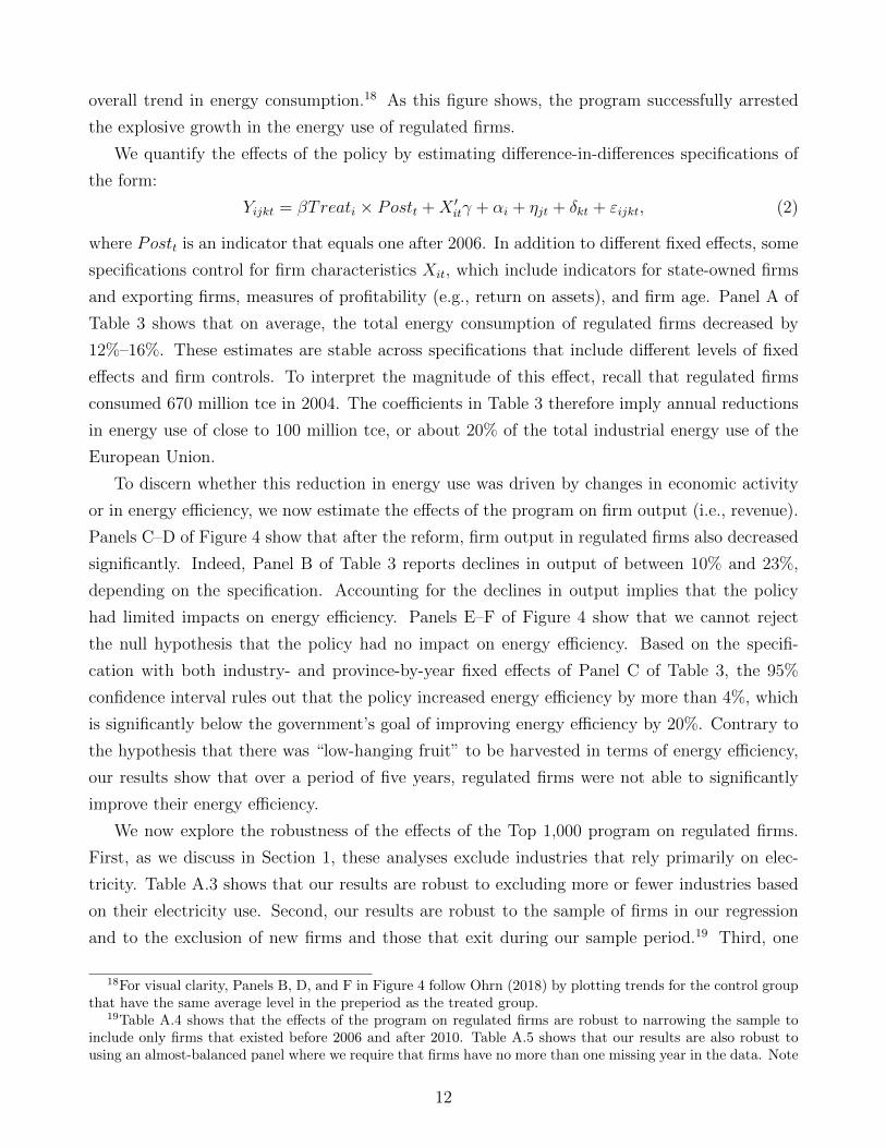
We quantify the effects of the policy by estimating difference-in-differences specifications of

the form:

Yijkt = βTreati × Postt +X ′itγ + αi + ηjt + δkt + εijkt, (2)

where Postt is an indicator that equals one after 2006. In addition to different fixed effects, some

specifications control for firm characteristics Xit, which include indicators for state-owned firms

and exporting firms, measures of profitability (e.g., return on assets), and firm age. Panel A of

Table 3 shows that on average, the total energy consumption of regulated firms decreased by

12%–16%. These estimates are stable across specifications that include different levels of fixed

effects and firm controls. To interpret the magnitude of this effect, recall that regulated firms

consumed 670 million tce in 2004. The coefficients in Table 3 therefore imply annual reductions

in energy use of close to 100 million tce, or about 20% of the total industrial energy use of the

European Union.

To discern whether this reduction in energy use was driven by changes in economic activity

or in energy efficiency, we now estimate the effects of the program on firm output (i.e., revenue).

Panels C–D of Figure 4 show that after the reform, firm output in regulated firms also decreased

significantly. Indeed, Panel B of Table 3 reports declines in output of between 10% and 23%,

depending on the specification. Accounting for the declines in output implies that the policy

had limited impacts on energy efficiency. Panels E–F of Figure 4 show that we cannot reject

the null hypothesis that the policy had no impact on energy efficiency. Based on the specifi-

cation with both industry- and province-by-year fixed effects of Panel C of Table 3, the 95%

confidence interval rules out that the policy increased energy efficiency by more than 4%, which

is significantly below the government’s goal of improving energy efficiency by 20%. Contrary to

the hypothesis that there was “low-hanging fruit” to be harvested in terms of energy efficiency,

our results show that over a period of five years, regulated firms were not able to significantly

improve their energy efficiency.

We now explore the robustness of the effects of the Top 1,000 program on regulated firms.

First, as we discuss in Section 1, these analyses exclude industries that rely primarily on elec-

tricity. Table A.3 shows that our results are robust to excluding more or fewer industries based

on their electricity use. Second, our results are robust to the sample of firms in our regression

and to the exclusion of new firms and those that exit during our sample period.19 Third, one

18For visual clarity, Panels B, D, and F in Figure 4 follow Ohrn (2018) by plotting trends for the control groupthat have the same average level in the preperiod as the treated group.

19Table A.4 shows that the effects of the program on regulated firms are robust to narrowing the sample toinclude only firms that existed before 2006 and after 2010. Table A.5 shows that our results are also robust tousing an almost-balanced panel where we require that firms have no more than one missing year in the data. Note

12

potential concern is that our results may be influenced by other, concurrent policies. Appendix

B clarifies that this is not the case by showing that our estimates are independent of the effects of

other pollution monitoring policies. As we show in Table A.6, these policies did not significantly

impact the operations of Top 1,000 firms, and our results are robust to excluding firms that are

part of these other programs. Finally, we explore the potential for heterogeneous effects across

industries. Given the small number of regulated firms in each industry, we estimate heteroge-

neous effects across broad industry groups. Table A.7 shows similar effects of the program across

different industry groups.20

The effects of the policy on regulated firms paint a picture of mixed success. On the one

hand, the regulation succeeded in achieving a meaningful reduction in the energy use of energy-

intensive firms. However, this reduction did not come about through a significant increase in

energy efficiency, which—while not directly targeted—was one of the underlying intents of the

policy. The next section studies whether conglomerates avoided the burden of the regulation by

shifting economic activity to related parties.

3 Spillover Effects of the Policy through Ownership

Networks

Regulated firms have strong incentives to shift production to related parties. By shifting pro-

duction, conglomerates can partially offset declines in economic activity in regulated firms. Such

shifting also allows conglomerates to comply with the letter of the regulation—if not with its

intent—without having to invest in potentially costly improvements to energy efficiency.

To measure the empirical importance of conglomerate spillovers, we use CARD data on the

ownership networks of regulated firms to identify firms that may have indirectly expanded as a

consequence of the Top 1,000 regulation. We then use matching methods to identify control firms

that were (1) not part of the Top 1,000 program, (2) not related to a regulated firm, and (3) in the

same industry and of similar size (measured in output) in the years prior to the regulation. Using

these firms as controls, we then conduct event-study and difference-in-differences analyses using

specifications similar to those in Equations (1) and (2).21 In this setting, the Treati variable is

now an indicator of whether a firm is related to a Top 1,000 firm. As we discuss in Section 1,

that due to the survey nature of the CESD data, our sample is substantially smaller in this case. Nonetheless,these results show that our estimates are not driven by firms entering the sample or ceasing operations.

20We also explore the effects of the program on other outcomes. In Table A.8 and Figure A.3, we show thatregulated firms experienced a decline in the probability of investing after the regulation was enacted. Additionally,we test the Porter and van der Linde (1995) hypothesis by examining whether firms became more innovative afterthe regulation. Figure A.4 shows no increase in the filing of patents related to energy efficiency in regulated firms.

21Specifically, we use one-to-one matching within 4-digit industries based on the Euclidean distance in outputlevels before the policy. To ensure that matches are comparable to related firms, we drop 5% of observations withthe least comparable matches. As we show below, our results are robust to using alternative matching methods.

13

we focus our study of spillovers on related firms in the same 4-digit industry as the regulated

firm. This restriction follows from the logic that only firms selling products similar to those of

the regulated firms may be able to make up for the production decline in Top 1,000 firms.

Figure 5 plots the results of these event-study analyses using ASIF data. Panel A shows that

prior to the regulation, related firms had output trends similar to those of unrelated firms. After

the regulation, firms related to Top 1,000 firms saw significant increases in output that persisted

for several years. The last column of Panel A of Table 4 shows that related firms expanded by

13%, on average, after the regulation. This table also shows that we obtain very similar results

across specifications with different levels of fixed effects and with firm-level controls.

To gauge the magnitude of these spillover effects, it is important to account for the number

of related parties of each regulated firm and for their relative size. On average, Top 1,000 firms

have 2.45 related parties. However, since the average related firm is only 19.3% as large as

its regulated counterpart, we calculate that conglomerates could only shift close to 41% of the

output decline in regulated firms.22 This result is informative for a couple of reasons. First,

this result shows that conglomerates were not able to fully circumvent the regulation. Second,

combined with the null effect of the program on the energy efficiency of regulated firms, this

result shows that firms were unable or unwilling to increase their energy efficiency in production

processes even if this meant losing profits to competitors.

The result that related firms display an increase in economic activity is robust to a number

of checks. First, we show that we obtain similar results when we use the entropy balancing

method of Hainmueller (2012) to find controls for related firms (see Figure A.5 and Tables

A.9–A.10).23 Second, we show that only those related firms operating in regulated firms’ own

narrowly defined industries—and that could thus possibly produce substitute output—increased

their economic activity. Indeed, Panel B of Figure 5 and Panel B of Table 4 show no impact

on the output of related firms operating outside the 4-digit industry of the regulated firm (but

still in the same 2-digit industry). This placebo test rules out the possibility that firms related

to large conglomerates saw increases in economic activity after 2007, say, in response to the

financial crisis or other shocks or trends. Third, these results are robust to alternative definitions

of ownership networks. Table A.11 shows similar spillover effects when we drop related firms

22Using the estimate on related firms from column (4) of Panel A of Table 4 of 12.7%, we calculate that theoverall increase in related firms amounted to 6%(≈ 2.45× 19.3%× 12.7%) of the output of regulated firms. Thisincrease is 41% of the comparable 14.5% decrease from column (4) of Panel B of Table 3. Using estimates fromthe specifications in columns (3), we obtain an estimate of 27%. (i.e., 27% ≈ 2.45× 19.3%× 11.8%/20.4%). Wecan also gauge the sensitivity of this estimate to the measurement of business networks. Supposing that regulatedfirms had an average of 3 related firms, spillovers would account for 51% of the output decline in regulated firms.

23Our estimates of spillover effects are also not driven by the entry and exit of related firms. To find asuitable control, our matching analysis requires firms to have existed prior to 2006. Moreover, because we mapbusiness networks in 2018, our estimates include the effects on firms that joined regulated business groups afterthe program.

14

with ownership changes between 2007 and 2018, when we restrict the sample by requiring 51%

ownership at each link, and when we expand the sample to include 6 levels of relations and 20%

ownership stakes. Fourth, these results are robust to dropping firms in power generation (see

Table A.12 and Figure A.6). Finally, we assuage concerns that our results may be affected by

data quality issues by showing similar effects when we rely on tax data to measure the output

of related firms (see Figure A.7 and Table A.13).24

We now explore the potential for heterogeneous spillovers across related firms. Panel C of

Table 4 shows that related firms in higher terciles of the size distribution display larger increases in

output. This result suggests that larger related firms were more able to expand or, alternatively,

that these firms had larger installed production capacity. As in our analysis of regulated firms,

we explore potential heterogeneous effects across industries. Table A.15 shows no significant

differences in how related firms in different industries responded to the program. Finally, we

explore the possibility that the regulation shifted economic production and related emissions to

more populated or more polluted areas. As we show in Appendix C, the spillover effects of the

regulation do not disproportionately shift production to areas with higher population density or

with higher preexisting levels of industrial emissions.

Having established that conglomerates shifted output across related parties, we now explore

whether these firms also saw changes in energy use and energy efficiency. Panels C and D of

Figure 5 report these results using data from the CESD. Panel C shows that related firms saw

an increase in energy use after the regulation. Panel A of Table 5 shows that energy use in

related firms increased by 30%–32% after the regulation. Note that the number of observations

in this panel is smaller than that in Panel A of Table 4. This is because related firms are overall

smaller and only the larger related firms are included in the CESD. These larger effects are

consistent with our results in Panel C of Table 4 showing larger spillover effects on larger related

firms. While the available data include firms across all affected industries, caution is warranted

in ascribing these increases in energy use to all related firms. Panel D of Figure 5 and Panel

B of Table 5 show that these firms did not experience statistically significant changes in energy

efficiency.

Overall, we find robust evidence that conglomerates shifted production across related parties.

On average, this shifting behavior allowed conglomerates to recover about 40% of the output

reduction in regulated firms. As we show in Section 6, the ability to shift production to related

firms diminishes the aggregate energy savings and lowers the shadow cost of the regulation.

24We also find positive spillover effects on other measures of economic activity. Table A.14 shows estimates ofpositive spillover effects on sales, profits, capital and labor (see Figure A.8 for corresponding event studies).

15

Market-level Spillovers

Since related parties could not make up the entire output loss of Top 1,000 firms, other firms

in regulated industries may have been indirectly affected by the energy saving program due to

reduced competition. To examine this indirect effect of the regulation, we estimate the following

difference-in-differences specification:

Yijt = βspilloverj × Postt +X ′itγ + αi + τt + εijt, (3)

where spilloverj is the proportion of the total energy saving targets of Top 1,000 firms for industry

j in total energy consumption of industry j in 2004. To interpret the coefficient β as the average

spillover effect, we normalize the spilloverj variable by the average exposure across regulated

industries. Since the variation in the independent variable is at the industry-year level, we do

not include industry-by-year fixed effects in this regression. We instead use firm fixed effects

and year fixed effects only and we additionally control for overall output and energy use at the

industry-year level.25 Finally, to ensure that market-level spillovers are not contaminated by

ownership-network spillovers, we exclude firms related to Top 1,000 firms from this specification.

Figure 6 shows that unregulated firms in industries with stricter regulation increased their

output significantly after the policy was implemented. Table 6 shows that across all industries,

the average market-level spillover led to a 7%–8% increase in the output of unregulated firms.

The regressions in the first two columns of this table include both regulated and unregulated

industries. We find similar increases (8%) when we include only firms in regulated industries.

In this case, the identifying variation is driven solely by differences in regulation intensity across

industries.26

These results yield a couple of insights. First, the findings further confirm our previous

estimates that related parties were not able to make up for the full output loss of Top 1,000 firms.

Second, a full accounting of the spillover effects of the regulation needs to include both within-

conglomerate spillovers and market-level spillovers. Third, a potential limitation of the difference-

in-differences analyses is that their interpretation depends on the strength of conglomerate and

market spillovers. The next section builds on these insights by proposing a model of conglomerate

production. The model clarifies the interpretation of our reduced-form estimates in the presence

of market and conglomerate spillovers, computes the aggregate effects of the Top 1,000 program,

and allows us to consider the effects of alternative policies.

25Note that the variation in spilloverj is absorbed in our previous specifications that include industry-by-yearfixed effects. By controlling for industry-level aggregates, the coefficient β in Equation 3 captures the impact ofthe regulation on the market share of unregulated firms.

26As with our previous analyses, we confirm that our results are not driven by firm entry. Specifically, in TableA.16, we report similar estimates of market-level spillovers when we restrict the sample to firms in operation priorto 2006.

16

4 A Model of Conglomerates with Regulation

This section presents an industry equilibrium model of conglomerate production that is consis-

tent with the cross-sectional data patterns and reduced-form responses to the policy of energy

regulation. Appendix D provides detailed derivations of the model results.

4.1 Demand and Technology

Our industry equilibrium model draws the structure of product differentiation and monopolistic

competition from Melitz (2003). We consider an individual sector with an exogenous aggregate

expenditure R. The representative consumer has CES preferences over a continuum of varieties

ω ∈ Ω:

U =

[∫ω∈Ω

q(ω)ρdω

]1/ρ

,

where q(ω) represents the consumption level of variety ω and σ = 1/(1 − ρ) > 1 denotes the

elasticity of substitution between varieties.27

Utility maximization by the representative consumer yields the following residual demand

curve for each variety ω:

q(ω) = RP σ−1p(ω)−σ,

where P = [∫ω∈Ω

p(ω)1−σdω]1

1−σ is the aggregate price index.28

We define a conglomerate in our model by the presence of a variety ω that can be manu-

factured by multiple affiliates.29 Each conglomerate starts with a central producer—the model

counterpart of a Top 1,000 firm. Conglomerates have heterogeneous production efficiencies φ,

which are drawn from the distribution G(φ) with density g(φ).

Production at each affiliate i requires capital ki, energy ei, and variable inputs li. Energy and

variable inputs are combined using Leontief technology li = minli, eiνi, where νi is the affiliate’s

energy efficiency. The assumption that energy and variable inputs are perfect complements

follows recent work in this area (e.g., van Biesebroeck, 2003; Fabrizio et al., 2007; Gao and

Van Biesebroeck, 2014; Ryan, 2018).30 Production at affiliate i is then qi = φilαli k

αki , which is

27Since the regulated firms produce raw and intermediate materials, one can view the representative consumeras a stand-in for the downstream industry.

28This market structure implicitly assumes that this industry is not characterized by dominant firms that mayact strategically. This is a reasonable assumption in our setting since we study manufacturing industries that,even when narrowly defined, feature a large number of firms and that serve a national market.

29This assumption implies that the outputs of related firms are perfect substitutes. We relax this assumptionin Section 7.4, where we allow the outputs of related firms to be imperfect substitutes.

30Fabrizio et al. (2007); Gao and Van Biesebroeck (2014) adopt this assumption from van Biesebroeck (2003)in the context of energy generation. Gao and Van Biesebroeck (2014) study the case of China. Ryan (2018)estimates a production function with energy using data from India and finds that energy and unskilled labor areclose to being perfect complements.

17

subject to decreasing returns to scale, i.e., α = αk + αl < 1. The decreasing-returns-to-scale

assumption is consistent with the literature on span of control. Intuitively, conglomerates may

operate more firms as a way to escape decreasing returns to scale and as a way to share production

knowledge φ across firms. However, as we show in Panel A of Figure 3, conglomerates are not

able to replicate the same scale across related firms. To match this fact, we assume that the

productivity of the ith affiliated firm is δi−1φ. This assumption can be interpreted as either a

limit on the span of managerial control or as a measure of imperfect knowledge-sharing across

firms. Finally, each manufacturing establishment incurs a fixed outlay of capital denoted by f .

This assumption is motivated by the fact that conglomerates have a finite number of affiliates.

We consider the conglomerate’s problem in two stages. Prior to the regulation, conglomerates

observe their productivity φ and optimally choose the number of affiliated firms n and the amount

of capital kini=1 and variable inputs lini=1 for each affiliate.31 After the regulation, since capital

is quasifixed, the conglomerate adjusts its variable inputs to maximize profits. We initially assume

energy efficiency is constant and fixed (i.e., νi = 1 for all firms) but consider costly investments

to improve energy efficiency and heterogeneous efficiencies in Sections 7.1 and 7.2.

4.2 Profit Maximization

The conglomerate takes the prices of energy pe, capital r, and the variable input bundle w as

given. Given the Leontief technology, the conglomerate sets li = ei so that the cost of intermediate

inputs is w + pe. Holding the number of affiliates n constant, the conglomerate maximizes

π(φ, n) = maxlini=1,kini=1

R1−ρP ρ

[n∑i=1

φδi−1kαki lαli

]ρ− (w + pe)

n∑i=1

li − rn∑i=1

ki

. (4)

For a firm i, the first-order conditions for li and ki imply that li = αlαk

r(w+pe)

ki. Substituting this

expression and comparing the first-order conditions for k1 and ki, we obtain the following result.

Proposition 1 (Within-Conglomerate Distribution). Absent regulation, the inputs and the out-

put of producers in a conglomerate follow a decreasing geometric sequence given by

qiq1

=kik1

=lil1

=eie1

= δi−11−α . (5)

The within-conglomerate distribution described in Proposition 1 is broadly consistent with

the empirical pattern in Panel A of Figure 3, where the average output of the second-largest

affiliate in a conglomerate is less than 30% of that of the largest one and where the output of

other affiliated producers in the conglomerate decreases exponentially with their rank i. Equation

5 links this distribution to two model parameters. First, the size gap among affiliates is larger if

31Conglomerates can choose n = 0, which we interpret as an exit decision.

18

within-group knowledge depreciation is more severe (lower δ). Second, if firms are closer to having

constant-returns-to-scale production (α is closer to one), the conglomerate concentrates more

activity in its top producer, which increases the dispersion of the within-group size distribution.

To consider the choice of total capital Kn =∑n

i ki, define the conglomerate’s total produc-

tivity φ∆n = φ[∑n

i=1(δi−1)1

1−α ]1−α and the constant Cπ = (1−αρ)[(

ραlw+pe

)αlρ (ραkr

)αkρ] 11−αρ

. We

reformulate Equation 4 using the results of Proposition 1 so the optimal choice of capital Kn

solves

π(φ, n) = maxKn

R1−ρP ρC1−αρ

π

(1− αρ)1−αρ

(ραkr

)−αρ(φ∆n)ρKαρ

n − r(α

αk

)Kn

.

The optimal capital Kn and the firm profits for a conglomerate of size n are then

Kn =R

1−ρ1−αρP

ρ1−αρCπ

(1− αρ)

ραkr

(φ∆n)ρ

1−αρ and π(φ, n) = R1−ρ1−αρP

ρ1−αρCπ (φ∆n)

ρ1−αρ .

Consider now the optimal number of affiliates. The conglomerate adds an affiliate if

π(φ, n+ 1)− π(φ, n)− fr = R1−ρ1−αρP

ρ1−αρCπ ×

[(φ∆n+1)

ρ1−αρ − (φ∆n)

ρ1−αρ

]− fr > 0. (6)

Adding a new affiliate can improve the conglomerate’s revenue and profit by lowering its overall

marginal cost curve. On the other hand, the conglomerate incurs a fixed cost of fr when adding

a new affiliate. While the marginal benefit of adding a new affiliate is increasing in φ, it is also

decreasing in the number of existing affiliates n. Since the fixed cost is the same for all affiliates,

Equation 6 guarantees the existence of a cutoff value φn, where conglomerates with efficiency

φ > φn operate at least n affiliated producers.

Proposition 2 (Optimal Conglomerate Size). Without regulation, the optimal number of firms

in a conglomerate n is nondecreasing in its fundamental efficiency φ. For n > 1, a conglomerate

chooses to have n affiliated producers when φn ≤ φ < φn+1, where

φn+1 =(fr)

1−ραρ

R1−ρρ PC

1−ραρ

π

(∆

ρ1−ραn+1 −∆

ρ1−ραn

) 1−ραρ

. (7)

Let π(φ) = maxn π(φ, n)−nfr be the profit for a conglomerate of efficiency φ at the optimal

number of affiliates. The prediction from Proposition 2 is consistent with the observation in

Panel B of Figure 3 that conglomerates with higher efficiency have, on average, a larger number

of affiliated firms.

4.3 Equilibrium and Welfare

The unique equilibrium of the model is characterized by product-market clearing, the zero cut-off

profit condition, and the free entry condition.

19

With M denoting the mass of active firms, the aggregate price index is given by

P =

[∫ ∞φ1

p(φ)1−σ g(φ)M

1−G(φ1)dφ

] 11−σ

. (8)

Conglomerates operate whenever

π(φ) ≥ 0 ⇒ φ ≥ φ1 =(fr)

1−ραρ

R1−ρρ PC

1−ραρ

π

. (9)

Equation 9 shows that only firms with φ > φ1 choose to participate in the market.32

To enter the market, an entrepreneur pays an entry cost rfe. Upon entry, the efficiency of

the conglomerate φ is realized. Since the conglomerate operates only if φ > φ1, the free entry

condition is given by ∫ ∞φ1

π(φ)g(φ)dφ− rfe = 0. (10)

An equilibrium is given by the exit threshold φ1 and the mass of active conglomerates M

such that (1) conglomerates make optimal allocation and size decisions, (2) the product market

clears, and (3) the zero profit and free entry conditions (Equations 9–10) are satisfied.

Welfare depends on consumption utility and on the utility costs of carbon emissions from

energy use. The CES preferences of the representative consumer imply that indirect utility is

given by RP, where R is total expenditure. Utility is decreasing in total emissions βE, where E

denotes aggregate energy use and β captures the carbon dioxide emitted per unit of energy. We

assume that welfare takes the form

W =

(R

P

)1−κ(1

βE

)κ, (11)

where the parameter κ captures the social welfare losses from emissions.33

4.4 Effects of the Top 1,000 Program

We denote outcomes in the unregulated equilibrium with an asterisk to differentiate them from

those in the regulated equilibrium. Since the Top 1,000 program targeted very large firms, we

assume that only conglomerates with φ above an efficiency level φ are subject to the regulation.

The regulation sets a proportional input quota for the largest firm in each conglomerate, which is

the model counterpart of a Top 1,000 firm. Specifically, the energy use of regulated firms cannot

exceed e1(φ) = ξe∗1(φ), where ξ < 1 and e∗1 is the unregulated optimal energy use. At the time of

32φ1 is the minimum efficiency for a single-firm conglomerate, so that π(φ1) = 0.33See Shapiro (2021) for a similar formulation of social welfare. Since we find that the regulation does not

significantly shift the geographic distribution of energy use, our welfare measure does not account for the locationof emissions (e.g., as in Shapiro, 2016).

20

the regulation, the conglomerate’s capital allocations k∗i ni=1 are quasifixed, but it can respond

by adjusting its use of inputs li, eini=1. Our model characterizes firm-level, conglomerate-level,

and industry-wide effects of the program.

We first study how the regulation impacts firm-level production decisions. To do so, we

substitute the result from Proposition 1 that ki = δi−11−αk1 into Equation 4, define φ∗ = φ(k∗1)αk ,

and let λ be the Lagrange multiplier associated with the regulatory constraint.34 The first-order

conditions for li (1 ≤ i ≤ n) are then

∂π

∂li= R1−ρP ρ︸ ︷︷ ︸

Market Demand

ρ

[φ∗

n∑i=1

δ(i−1)(1−αl)

1−α lαli

]ρ−1

︸ ︷︷ ︸Residual Revenue

φ∗δ(i−1)(1−αl)

1−α αl(li)αl−1︸ ︷︷ ︸

Marginal Product

= w + pe + λ(φ)I[i = 1]︸ ︷︷ ︸Shadow Cost

of Regulation

. (12)

An important insight of this expression is that conglomerates internalize the marginal product of

inputs across firms through the residual revenue term, which is common to all firms in the con-

glomerate. The impact of energy regulations on the residual revenue term is key to understanding

the difference between within-conglomerate and market-level spillovers.

This equation shows that the regulation distorts the allocation of inputs within a conglomerate

by adding a shadow cost λ(φ) to the input of the regulated firm. Because conglomerates with

more affiliates can shift more production to related parties, conditional on being regulated, more

efficient conglomerates (those with a higher φ) are subject to a smaller shadow cost λ(φ). Since

only conglomerates with φ > φ are part of the Top 1,000 program, the regulation also distorts

input use across conglomerates.

The following proposition shows that the regulation leads conglomerates to allocate more

inputs to the unregulated firms than in the case without the regulation.

Proposition 3 (Within-Conglomerate Distribution under Regulation). Under the Top 1,000

regulation, the inputs and the output of producers follow the sequences given by

eje2

=ljl2

=qjq2

= δj−21−α for j > 2,

eie1

=lil1

= δi−11−α ×

[1 +

λ(φ)

w + pe

] 11−αl

andqiq1

= δi−11−α ×

[1 +

λ(φ)

w + pe

] αl1−αl

for i > 1.

Even though conglomerates substitute production across firms, the regulation leads to an over-

all reduction in the conglomerate’s output. The following proposition describes the conglomerate-

level effects of the regulation on output and energy use.

34Note that k∗1 = K∗n(∆n)−11−α .

21

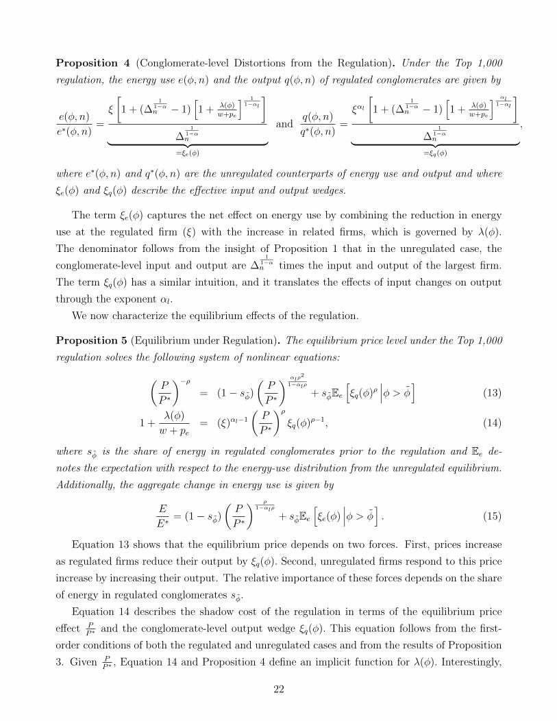
Proposition 4 (Conglomerate-level Distortions from the Regulation). Under the Top 1,000

regulation, the energy use e(φ, n) and the output q(φ, n) of regulated conglomerates are given by

e(φ, n)

e∗(φ, n)=

ξ

[1 + (∆

11−αn − 1)

[1 + λ(φ)

w+pe

] 11−αl

]∆

11−αn︸ ︷︷ ︸

=ξe(φ)

andq(φ, n)

q∗(φ, n)=

ξαl[1 + (∆

11−αn − 1)

[1 + λ(φ)

w+pe

] αl1−αl

]∆

11−αn︸ ︷︷ ︸

=ξq(φ)

,

where e∗(φ, n) and q∗(φ, n) are the unregulated counterparts of energy use and output and where

ξe(φ) and ξq(φ) describe the effective input and output wedges.

The term ξe(φ) captures the net effect on energy use by combining the reduction in energy

use at the regulated firm (ξ) with the increase in related firms, which is governed by λ(φ).

The denominator follows from the insight of Proposition 1 that in the unregulated case, the

conglomerate-level input and output are ∆1

1−αn times the input and output of the largest firm.

The term ξq(φ) has a similar intuition, and it translates the effects of input changes on output

through the exponent αl.

We now characterize the equilibrium effects of the regulation.

Proposition 5 (Equilibrium under Regulation). The equilibrium price level under the Top 1,000

regulation solves the following system of nonlinear equations:(P

P ∗

)−ρ= (1− sφ)

(P

P ∗

) αlρ2

1−αlρ

+ sφEe[ξq(φ)ρ

∣∣∣φ > φ]

(13)

1 +λ(φ)

w + pe= (ξ)αl−1

(P

P ∗

)ρξq(φ)ρ−1, (14)

where sφ is the share of energy in regulated conglomerates prior to the regulation and Ee de-

notes the expectation with respect to the energy-use distribution from the unregulated equilibrium.

Additionally, the aggregate change in energy use is given by

E

E∗= (1− sφ)

(P

P ∗

) ρ1−αlρ

+ sφEe[ξe(φ)

∣∣∣φ > φ]. (15)

Equation 13 shows that the equilibrium price depends on two forces. First, prices increase

as regulated firms reduce their output by ξq(φ). Second, unregulated firms respond to this price

increase by increasing their output. The relative importance of these forces depends on the share

of energy in regulated conglomerates sφ.

Equation 14 describes the shadow cost of the regulation in terms of the equilibrium price

effect PP ∗

and the conglomerate-level output wedge ξq(φ). This equation follows from the first-

order conditions of both the regulated and unregulated cases and from the results of Proposition

3. Given PP ∗, Equation 14 and Proposition 4 define an implicit function for λ(φ). Interestingly,

22

the shadow cost λ(φ) and the conglomerate-level wedge ξq(φ) are step functions of φ. While

these functions depend on the number of affiliates in a conglomerate n, they are constant across

conglomerates of the same size but with different values of φ.35 Intuitively, this result is a

consequence of the fact that the energy cap in the regulation is proportional to the firm’s prior

energy use, which itself depends on φ.

The equilibrium under the regulation is then determined by a single shadow cost for every

value of n along with the equilibrium price PP ∗, which greatly facilitates the computation of the

new equilibrium. Equation 15 then shows that the equilibrium effect on energy depends on the

net change in conglomerate energy use ξe(φ) and the market leakage to unregulated firms.

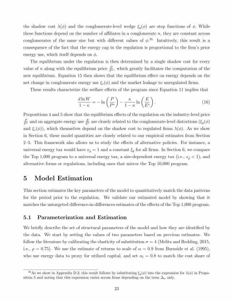
These results characterize the welfare effects of the program since Equation 11 implies that

d lnW

1− κ= − ln

(P

P ∗

)− κ

1− κln

(E

E∗

). (16)

Propositions 4 and 5 show that the equilibrium effects of the regulation on the industry-level pricePP ∗

and on aggregate energy use EE∗

are closely related to the conglomerate-level distortions (ξq(φ)

and ξe(φ)), which themselves depend on the shadow cost to regulated firms λ(φ). As we show

in Section 6, these model quantities are closely related to our empirical estimates from Section

2–3. This framework also allows us to study the effects of alternative policies. For instance, a

universal energy tax would have sφ = 1 and a constant ξq for all firms. In Section 6, we compare

the Top 1,000 program to a universal energy tax, a size-dependent energy tax (i.e., sφ < 1), and

alternative forms or regulations, including ones that mirror the Top 10,000 program.

5 Model Estimation

This section estimates the key parameters of the model to quantitatively match the data patterns

for the period prior to the regulation. We validate our estimated model by showing that it

matches the untargeted difference-in-differences estimates of the effects of the Top 1,000 program.

5.1 Parameterization and Estimation

We briefly describe the set of structural parameters of the model and how they are identified by

the data. We start by setting the values of two parameters based on previous estimates. We

follow the literature by calibrating the elasticity of substitution σ = 4 (Melitz and Redding, 2015,

i.e., ρ = 0.75). We use the estimate of returns to scale of α = 0.9 from Burnside et al. (1995),

who use energy data to proxy for utilized capital, and set αl = 0.8 to match the cost share of

35As we show in Appendix D.2, this result follows by substituting ξq(φ) into the expression for λ(φ) in Propo-sition 5 and noting that this expression varies across firms depending on the term ∆n only.

23

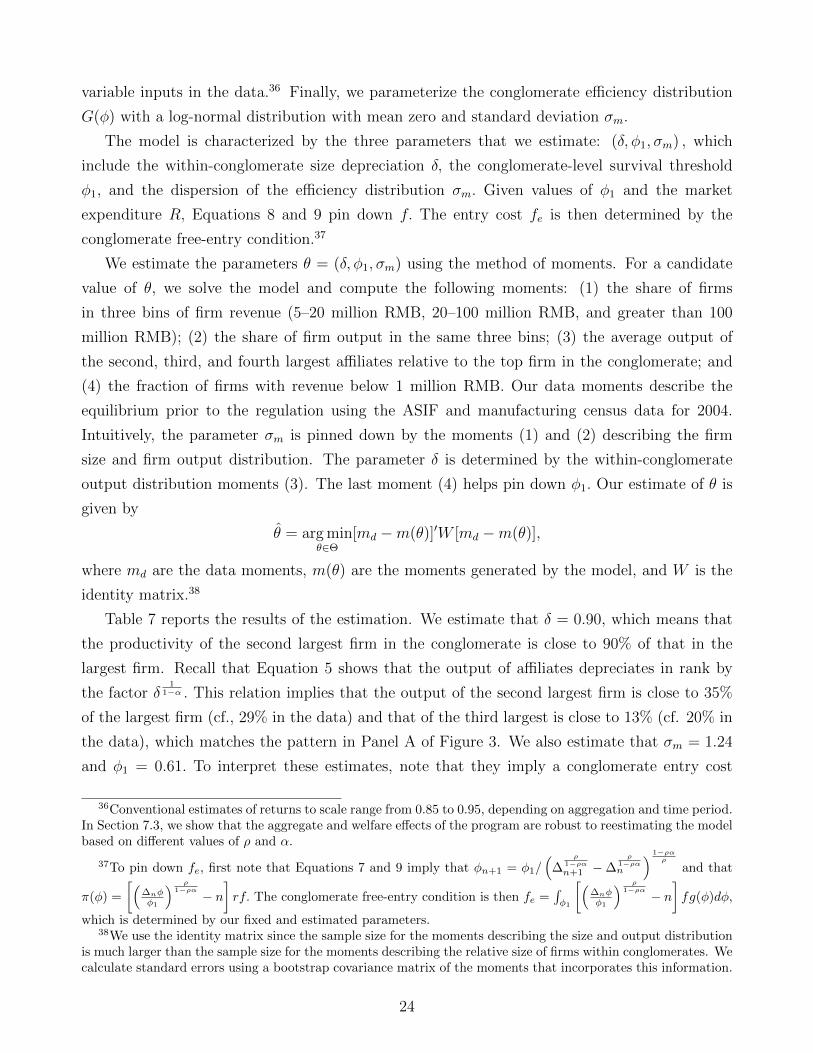
variable inputs in the data.36 Finally, we parameterize the conglomerate efficiency distribution

G(φ) with a log-normal distribution with mean zero and standard deviation σm.

The model is characterized by the three parameters that we estimate: (δ, φ1, σm) , which

include the within-conglomerate size depreciation δ, the conglomerate-level survival threshold

φ1, and the dispersion of the efficiency distribution σm. Given values of φ1 and the market

expenditure R, Equations 8 and 9 pin down f. The entry cost fe is then determined by the

conglomerate free-entry condition.37

We estimate the parameters θ = (δ, φ1, σm) using the method of moments. For a candidate

value of θ, we solve the model and compute the following moments: (1) the share of firms

in three bins of firm revenue (5–20 million RMB, 20–100 million RMB, and greater than 100

million RMB); (2) the share of firm output in the same three bins; (3) the average output of

the second, third, and fourth largest affiliates relative to the top firm in the conglomerate; and

(4) the fraction of firms with revenue below 1 million RMB. Our data moments describe the

equilibrium prior to the regulation using the ASIF and manufacturing census data for 2004.

Intuitively, the parameter σm is pinned down by the moments (1) and (2) describing the firm

size and firm output distribution. The parameter δ is determined by the within-conglomerate

output distribution moments (3). The last moment (4) helps pin down φ1. Our estimate of θ is

given by

θ = arg minθ∈Θ

[md −m(θ)]′W [md −m(θ)],

where md are the data moments, m(θ) are the moments generated by the model, and W is the

identity matrix.38

Table 7 reports the results of the estimation. We estimate that δ = 0.90, which means that

the productivity of the second largest firm in the conglomerate is close to 90% of that in the

largest firm. Recall that Equation 5 shows that the output of affiliates depreciates in rank by

the factor δ1

1−α . This relation implies that the output of the second largest firm is close to 35%

of the largest firm (cf., 29% in the data) and that of the third largest is close to 13% (cf. 20% in

the data), which matches the pattern in Panel A of Figure 3. We also estimate that σm = 1.24

and φ1 = 0.61. To interpret these estimates, note that they imply a conglomerate entry cost

36Conventional estimates of returns to scale range from 0.85 to 0.95, depending on aggregation and time period.In Section 7.3, we show that the aggregate and welfare effects of the program are robust to reestimating the modelbased on different values of ρ and α.

37To pin down fe, first note that Equations 7 and 9 imply that φn+1 = φ1/(

∆ρ

1−ραn+1 −∆

ρ1−ραn

) 1−ραρ

and that

π(φ) =

[(∆nφφ1

) ρ1−ρα − n

]rf. The conglomerate free-entry condition is then fe =

∫φ1

[(∆nφφ1

) ρ1−ρα − n

]fg(φ)dφ,

which is determined by our fixed and estimated parameters.38We use the identity matrix since the sample size for the moments describing the size and output distribution

is much larger than the sample size for the moments describing the relative size of firms within conglomerates. Wecalculate standard errors using a bootstrap covariance matrix of the moments that incorporates this information.

24

of fe = 8.9 million RMB (or about 1.1 million USD), which is reasonably commensurate with

average profit in the economy. The per-firm operating fixed cost is determined by the average

sales per conglomerate in the data, which implies that f = 44, 000 RMB. Panel A of Figure 7

shows that our model does a good job of fitting both the observed firm-size distribution and the

concentration of output prior to the regulation.

5.2 Model Response to the Top 1,000 Program

We need two additional parameters to implement the Top 1,000 program in our model. As

discussed in Section 4, our version of the regulation targets conglomerates with efficiency level φ

above φ. We choose the threshold φ to match the share of total energy consumed by regulated

firms within energy-intensive industries. Given our estimated parameters, the model implies

a value of φ = 9.29, which reproduces the fact that regulated firms account for 56% of total

energy consumption in energy-intensive industries. Finally, we take the policy intensity ξ from

the 11FYP, which targeted an energy reduction of 20%. For this reason, we set ξ = 0.8. Table 7

collects the model parameters.

We now use our estimated model to compute the effects of the Top 1,000 program. As in

Section 4.4, we assume conglomerates take the number of affiliates and capital allocation as

given. The new industry equilibrium ensures that (1) regulated conglomerates allocate variable

inputs optimally (as in Equation 12), (2) unregulated firms increase output to respond to the

increase in market prices, and (3) the product market clears (as in Equation 8).

Panel B of Figure 7 compares our difference-in-differences estimates to simulated model ana-

logues. The model does a remarkable job of matching the estimated effects on firm output. This

is true for regulated firms, related firms, and market-level spillovers. The model prediction of

the change in input use of regulated firms is within the 95% confidence interval of our empirical

estimate, but the model has a hard time fitting the effect on the energy use of related firms. This

may reflect the fact that, as we discuss in Section 3, this estimate is based on a smaller sample

of larger firms and may not be representative of the overall response. However, the model does

a good job of matching the effects of the program on the energy efficiency of both regulated

and related firms. Overall, these results show that our model can reproduce the effects of the

regulation on the output of regulated, related, and unrelated firms, which is remarkable since

these are all out-of-sample predictions of the model.

5.3 Using the Model to Interpret Difference-in-Differences Estimates

An important force in the model is that unregulated firms are impacted by the regulation through

the market spillover. This force contributes to the effects of the program on the equilibrium price

25

and aggregate energy use. We now use our model to understand how this market spillover impacts

our difference-in-differences estimates.

To see how the regulation in our model connects to our difference-in-differences analysis, note

that we can write conglomerate j’s revenue from affiliate i as follows:

ln Revenueij = ln(Production Shareij)︸ ︷︷ ︸Allocation Effect

+ ρ ln

(∑i∈j

qij

)︸ ︷︷ ︸Residual Revenue

+ ln(R1−ρP ρ)︸ ︷︷ ︸Market Demand

, (17)

where Production Shareij = qij/∑i∈jqij.

39 Equation 17 clarifies the three ways in which the Top

1,000 program impacts the revenue of regulated firms. First, when firm i is regulated, the

conglomerate is forced to reallocate inputs to other firms, which lowers the production share

in regulated firms. Panel A of Table 8 reports that in our model, the share of production in

regulated firms within a conglomerate decreases by 12.9%. Second, since the marginal cost goes

up at the conglomerate level, the market share of the conglomerate’s variety decreases, which

lowers the group’s residual revenue. Table 8 shows that regulated conglomerates see their residual

revenue decrease by 3.7%. Finally, the Top 1,000 program impacts the industry-level price P.

This price increase has a countervailing effect on the revenue of the regulated firm and lessens

the overall decline by 2.6%. Combining these three forces, our model implies that regulated firms

decreased their output by 14%.

Equation 17 also characterizes the impact of the regulation on the control firms in our

difference-in-differences analyses. Since these firms are not regulated or related to Top 1,000

firms, the regulation does not impact the within-conglomerate allocation of production. Control

firms see an increase in their residual and firm-level revenue as the market reallocates demand.

Table 8 shows that the residual revenue of control firms increases by 3.9%. As in the case of

regulated firms, unregulated firms also benefit from the equilibrium impact on market demand.

This discussion clarifies that our difference-in-differences estimates differ from the total effect

on Top 1,000 firms along two margins. First, the difference-in-differences estimator captures both

the within- and across-conglomerate reallocation of production. This leads to an overestimate of

the effect of the program on regulated firms of 3.9%. Second, since the market effect cancels out,

the difference-in-differences estimator does not capture the countervailing effect on the industry-

level price, which further overestimates the effect of the program by 2.6%.40

Similarly, our model allows us to decompose the estimates of the spillover effects of the

regulation through ownership networks. Panel B of Table 8 shows that related firms share the

residual revenue and market effect terms but have a positive allocation effect as their share of

39Equation 17 follows by multiplying conglomerate j’s inverse residual demand by affiliate i’s production.40Note that the first channel arises from the impact of the regulation on the control firms. The second channel

is an aggregate effect that is not identified by a difference-in-differences research design.

26

production within the conglomerate increases. The total effect on related firms is an output

increase of 19.3%. The effects on control firms is the same as that in Panel A. By ignoring the

positive market effect and subtracting the residual revenue effect on control firms, the difference-

in-differences estimator understates the spillover effect on related firms by 6.5%.

In addition to clarifying the interpretation of our reduced-form estimates, our model also

motivates an alternative approach that does not the depend on the residual revenue or market

effects. Specifically, consider a within-conglomerate difference-in-differences estimator where

treated firms are the regulated Top 1,000 firms and the control firms are unregulated firms in

the same conglomerate. Because Equation 17 shows that the residual revenue and market effect

are common to a given conglomerate, this estimator captures only the allocation effects of the

program. Figure 8 implements this within-conglomerate difference-in-differences approach. This

figure plots the results from an event-study specification similar to Equation 1 but where we

additionally include conglomerate-by-year fixed effects. Consistent with our previous results, we

find a significant decline in the output of Top 1,000 firms relative to that of other firms in their

same conglomerates. Table 9 reports estimates of these relative declines of between -31.5% and

-36.7%. As with our previous reduced-form effects, Panel B of Figure 7 shows that the model

matches this within-conglomerate effect very well. Moreover, Panel C of Table 8 confirms that

this effect is a combination of the allocation effects on regulated and related firms.

These insights highlight the importance of interpreting quasirandom estimates through the

lens of a model that accounts for within- and across-conglomerate reallocation of production as

well as equilibrium impacts on industry-level prices.

6 Policy Analysis

This section uses our estimated model to capture the effects of the Top 1,000 program by quan-

tifying the shadow cost to regulated firms, the aggregate effects on prices and energy use, and

the implied welfare trade-off of the program. We then consider the effects of alternative poli-

cies including program expansions (e.g., the Top 10,000 program) and the possibility that the

government can use information on business networks to improve energy regulation.

6.1 Effects of the Top 1,000 Program

Given that the shadow cost is the fundamental building block of our model outcomes, we first

quantify this cost of the policy.

27

6.1.1 Shadow Cost of the Policy

To compute the shadow cost of the policy, we solve for the regulated equilibrium as in Proposition

5. Panel A of Figure 9 plots the implied shadow cost as a function of efficiency φ. The blue line

plots the shadow cost of our computed Top 1,000 program. This shadow cost is zero for firms

with φ < φ and jumps to an average of 8.7% for regulated firms. Since the shadow cost has

the same scale as the cost of variable inputs, we can interpret this value as an equivalent tax

on variable inputs. While 8.7% might seem like a small number, recall that inputs constitute a

large tax base, especially relative to profits.41

A somewhat surprising feature of Panel A of Figure 9 is that the shadow cost appears to be

constant with respect to conglomerate productivity φ. Panel B of Figure 9 zooms in to show the

different shadow costs for regulated firms (i.e., φ > φ). As we discuss in Section 4, the shadow

cost is constant for conglomerates with the same number of related firms. This result follows

from the fact that the regulation is based on previous energy use, which is proportional to firm

productivity. When φ crosses the thresholds that define conglomerate size (Proposition 2), we

see that the shadow cost drops as conglomerates with more affiliates are more able to escape the

burden of the regulation. However, the differences in shadow costs are very small in comparison

to the overall difference between regulated and unregulated conglomerates. This small impact is

driven by the decay in within-conglomerate size, which implies that the marginal (nth) affiliate

may not be able to supplant a large fraction of the combined activity of all the other affiliates

(1 through n− 1) in the conglomerate.

We now validate the magnitude of the shadow cost using an additional implication of the

model. Recall the insight from Proposition 3 that the shadow cost is related to the within-

conglomerate output distribution after the regulation. Based on this insight, we can write the

output difference between the Top 1,000 firm and related firms as follows:

ln RevenueTop1000,jt − ln RevenueRelated,jt = ln (qTop1000,j)− ln

( ∑i 6=Top1000,j

qij

)

= − αl1− αl

ln

[1 +

λ(φ)

w + pe

]− ln

(∆

11−αn − 1

).

By definition, λ(φ) = 0 prior to the regulation, and ∆n is constant over time. Therefore, taking

a time difference of this expression shows that the within-conglomerate difference-in-differences

estimation identifies the term − αl1−αl

ln[1 + λ(φ)

w+pe

]. Using the estimate in the first column of

Table 9 of −34.3% and our value of αl = 0.80, we estimate a shadow cost of 8.95%.42 Given that

41Indeed, in models with constant marginal cost and with a similar value of σ, inputs are (σ − 1) = 3−timesas large as profits. An equivalent profit tax would then be 26.1%.

42This calculation follows from 1+ λ(φ)w+pe

= exp−β 1−αlαl = exp0.343 1−0.8

.8 = 1.0895. In principle, we identify

the average value of this quantity across firms. However, as we show in Figure 9, there is little variation in λ(φ).

28

the shadow cost plays an important role in our quantification exercises of the aggregate effects of

the program, it is reassuring that our estimated magnitude is consistent with the reduced-form

pattern of within-conglomerate reallocation of production.

Our model allows us to consider how different mechanisms impact the shadow cost of the

program. The top line of Panel A of Figure 9 shows that shutting down the market and con-

glomerate spillovers would increase the shadow cost to 15.6%. That is, the equilibrium price

increase and the ability to shift production to related firms lowered this mechanical effect by

almost 50%. The model also allows us to isolate how the ability of conglomerates to shift pro-

duction to related firms lowered the shadow cost of the regulation. The second line from the top

in Panel A of Figure 9 plots the shadow cost under the assumption that market prices adjust but

that regulated firms are not able to shift production to related parties. In this case, the shadow

cost of the regulation would be 11.2% of input costs, which is about 30% larger than the level in

the baseline case.43 These calculations showcase the importance of accounting for both market

and conglomerate spillovers in the measurement of the shadow cost of the regulation.

6.1.2 Aggregate and Welfare Effects of the Program

The analysis so far has focused on the distortionary aspects of the regulation. We now evaluate

the aggregate and welfare effects of the policy by considering the social welfare function of a

government concerned with both decreases in energy-use-related emissions and the impact of

distortions to production on consumption.44

We compute the aggregate effects of the program by solving the equilibrium conditions in

Proposition 5. Panel A of Figure 10 plots the effects of the Top 1,000 program in the space of

price increase and energy reduction. The red diamond in this figure shows that the Top 1,000

program led to a price increase of about 3.5% and an aggregate energy use reduction of close

to 4%. Equation 15 helps us understand how we obtain a 4% aggregate reduction in energy

use. First, we find that—including within-conglomerate reallocation—regulated conglomerates

reduced their energy use by 1−Ee[ξe(φ)

∣∣∣φ > φ]

= 5.8%. Second, the unregulated conglomerates

increased their energy use by close to 6.5%. Finally, we obtain the aggregate 4% decline by using

the fact that the share of energy in regulated conglomerates is sφ = 86%.45 Thus, even though

we find in Section 2 that Top 1,000 firms reduced their energy use by close to 100 million tce,

43This counterfactual assumes that, similar to unregulated firms, the production of related firms responds toequilibrium price increases. Restricting production in related firms to pre-regulation levels further increases theshadow cost to 14%.

44To match the short-run nature of our empirical analysis, we focus our discussion on the short-run effects ofthe policy, ignoring the entry of new conglomerates. Later changes to regulations and the overall environmentalso complicate the simulation of long-run impacts.

45The energy increase for unregulated firms is given by(PP∗

) ρ1−αlρ = (1.035)

0.751−0.8∗0.75 ≈ 1.065. Recall that

regulated firms account for 56% of energy use; accounting for related firms in the same conglomerate raises thisfraction to 86%. The aggregate effect is then −4% = ln(1.06 ∗ 0.14 + 0.942 ∗ 0.86).

29

the annual aggregate reduction—including conglomerate and market leakage—was closer to 48

million tce.46

While reducing energy use improves welfare by lowering related carbon emissions, the over-

all effects of the program on welfare also depend on how the program impacts consumption.

According to Equation 16, welfare increases when the aggregate price-to-energy use elasticity(i.e.,

− ln( PP∗ )

ln( EE∗ )

)is smaller than κ

1−κ . Given our aggregate estimates of the effects of the Top 1,000

program, we find that the program raises welfare as long as κ1−κ < 3.5

4= 0.875. That is, the

Top 1,000 program raises welfare as long as the government is willing to accept a 0.875% price

increase for every 1% reduction in energy use.

To obtain a more concrete interpretation of this condition, we calibrate κ by building on the

Cobb-Douglas intuition that exponents are related to expenditure shares. This intuition implies

that we can approximate κ as follows:

κ =Social Cost of Carbon× Carbon Emissions

Aggregate Income× 0.8.

The adjustment factor 0.8 comes from the fact that the Chinese government declared in the

11FYP that relative to its policy goals, the government was underspending on reducing emissions

by 20%. We implement this equation with 2006 data on overall emissions in China (6.38 billion

tons of carbon) and national income (2.752 trillion USD). We can then compute a value of

κ that corresponds to an estimate of the social cost of carbon (SCC). In the US, the Biden

administration has recently proposed using an SCC of $51 (IWG, 2021), although researchers

have recently argued for a higher value of $125 (Carleton and Greenstone, 2021). In contrast,

Germany has proposed an SCC value of $218.

Figure 10 implements this calibration by plotting black indifference curves where κ varies

according to different values of the SCC. That is, for a given SCC value, these lines plot combi-

nations of price and energy use changes that yield the same effect on welfare. The red diamond

in this figure shows that the Top 1,000 program lies on the indifference curve that corresponds

to an SCC of $160. This implies that this policy is desirable from a welfare perspective only if

policymakers use relatively higher values of the SCC.

6.2 Alternative Policies

We now use the model to consider alternative policies. We first explore different ways in which

the Top 1,000 program could be expanded or contracted. This exercise is motivated by the fact

that the Chinese government expanded the program to include more than 14,000 firms in the

46In Appendix D.2.3, we connect the model solution to our reduced-form estimates by showing that we cansolve an approximate version of the equilibrium using the value of λ that is implied by the within-conglomeratedifference-in-differences results.

30

Top 10,000 program in 2012. We then explore the effects of alternative regulations and energy

taxes to examine the degree to which the government can improve the regulation of energy.

We explore two ways to change the scope of the Top 1,000 program. First, we consider the

effect of varying the regulation threshold φ, which changes the number of firms affected by the

program. The blue dots in Panel A of Figure 10 show the effects of changing the size threshold,

φ. The first blue dot (left of the red diamond) considers the effect of decreasing the number

of regulated firms to cover only 50% of the energy use in the regulated industry (relative to

the current 56%). The second blue dot lowers φ so that the regulation instead covers 60% of

the industry’s energy use. As would be expected, we find larger energy decreases when the

program covers a larger fraction of overall energy use. However, Figure 10 shows that expanding

or contracting the number of firms in the program does not alter the fundamental trade-off that

the government faces between price increases and reductions in energy use.

An alternative way to change the scope of the Top 1,000 program is to increase or decrease the

energy use quota ξ. The maroon squares in Panel A of Figure 10 plot the effects of policies where

1 − ξ varies in 5% increments between 5% and 30%. Larger values of 1 − ξ lead to both larger

price increases and larger energy reductions. Taking both changes into account, we find that the

implied SCC increases with the required energy reduction and equals $165 when 1 − ξ = 30%.

This result is valuable since the government may be concerned about the administrative costs of

regulating a larger number of firms. Since increasing ξ and lowering φ have similar welfare effects,

it may therefore be desirable to place stricter energy use limits on fewer firms if the government

lacks the capacity or the funds to conduct additional energy audits.

We now consider the effects of an alternative policy that targets the energy use of all firms in

a given conglomerate.47 The orange crosses in Panel B of Figure 10 plot the effects of this type

of regulation for different values of ξ. These policies have the benefit that they do not distort

the within-conglomerate distribution of production. Panel A of Figure 9 shows that regulating

conglomerates has a lower shadow cost of 4.9% (instead of 8.7%). Such a policy is preferable

to the Top 1,000 program from a welfare perspective since it can achieve larger energy use

reductions for a given price increase. As we show in Panel B of Figure 10, this type of regulation

can yield a 4.36% reduction in aggregate energy use for the same price increase as the Top 1,000

program. This is a 10% increase from the energy reduction of the Top 1,000 program, which

corresponds to additional energy savings of 5 million tce. This policy improves welfare as long

as the SCC≥ $152. While this program would involve monitoring additional firms, the number

of firms related to Top 1,000 firms is less than 20% of the number of firms in the Top 10,000

program. These results show that the government can improve the regulation of energy by using

47We derive equilibrium conditions under these alternative regulations in Appendix E. To make this casecomparable, we model the effects of a regulation that limits the conglomerate-level use of energy to the levels ofthe Top 1,000 program. That is, we set ξ to values corresponding to ξe(φ) in the Top 1,000 program.

31

publicly available data on business networks to target conglomerates and that doing so would be

more effective than regulating additional unrelated firms, as with the Top 10,000 program.

Finally, we consider the effects of energy taxes. We first model the effects of a tax that

affects only firms in conglomerates with Top 1,000 firms (i.e., with φ > φ). Panel A of Figure 9

shows that we would obtain the same energy reduction as that under the Top 1,000 program by

taxing inputs at 4.9%.48 The green circles in Panel B of Figure 10 show that the effects of this

energy tax are very close to those of the conglomerate-level regulation.49 We further consider

the effects of a universal energy tax such that sφ = 100% instead of 86%. Panel B of Figure 10

shows that while a universal energy tax yields a slight improvement over the size-dependent tax

(SCC= $151), both the size-dependent tax and the conglomerate-level regulations imply very

similar welfare trade-offs.

The preferred policy solution for most economists on the regulation of carbon emissions related

to energy use is a universal carbon tax. In practice, this policy may not be feasible given legal,

administrative, or political constraints. The results in this section inform the efficacy and design

of a prominent real-world policy that regulates quantities and has incomplete coverage. We

find that the government can achieve similar aggregate effects by either expanding the program

through stricter regulations for current firms or increasing the number of firms in the program.

While the former has narrower coverage and generates larger inequities between regulated and

unregulated firms, the latter may require an increase in administration costs. We also find

that the government can improve the regulation of energy by targeting the ownership networks

of regulated firms. This policy increases aggregate energy savings by 10% without increasing

welfare costs. Moreover, this policy can be implemented with publicly available data, has a

lower administrative cost than the Top 10,000 program, and implies a welfare trade-off close to

that under a universal energy tax.

7 Extensions and Robustness

This section explores four extensions of our model. First, we consider the possibility of firms

responding to the regulation by investing in energy efficiency. Second, we consider how preex-

isting differences in energy efficiency across firms may alter the overall energy savings from the

program. Third, we study the robustness of our welfare calculations to alternative parameter-

48As with the Top 1,000 regulation, the shadow cost of the conglomerate-level regulation decreases slightly asthe number of related firms increases. In contrast, the shadow cost of the size-dependent energy tax is constantfor all firms affected by it. Since energy costs are close to 15% of variable input costs for Top 1,000 firms, theequivalent energy tax would be closer to 32.7%(≈ 4.9%

15% ).49It is worth noting that our quantification lacks two features that often motivate the use of taxes over

regulation. First, in our calculations, the revenue from the tax is not rebated to consumers; this calculationignores potential “double dividend” effects. Second, firms in our setting have homogeneous abatement costs; in asetting with heterogeneous abatement costs, a tax would additionally reallocate production to “cleaner” firms.

32

izations of the model. Finally, we extend our model to allow imperfect substitution between

products produced by firms in a given conglomerate.

7.1 Endogenous Energy Efficiency

Our baseline analysis assumes that in the short run, firms do not make any investments to improve

their energy efficiency. This assumption is consistent with our empirical results in Sections 2–

3. Following the intent of the Top 1,000 program, we now extend our model to allow firms to

respond by adjusting their energy efficiency. Appendix G.1 provides additional details of this

model extension.

We assume that the conglomerate can improve energy efficiency at firm i, νi, by spending

lic(νi), where c′(νi) > 0 and c′′(νi) ≥ 0. We can then restate the regulated conglomerate’s problem

as

π(φ, n) = maxlini=1,νini=1

R1−ρP ρ

[φ∗

n∑i=1

δ(i−1)(1−αl)

1−α lαli

]ρ−

n∑i=1

li

(w +

peνi

+ c(νi)

),

where we omit the cost of fixed capital. Absent the regulation, the conglomerate sets c′(ν∗)ν∗2 =

pe for all firms. This result implies that Propositions 1–2 continue to describe the equilibrium

prior to the regulation. To simplify the exposition, we assume that c(ν) = νγ

1+γ, where γ ≥ 1.

This implies that the effective price of energy inclusive of investments in energy efficiency ispeν∗

+ c(ν∗) = c′(ν∗)ν∗ + c(ν∗) = (ν∗)γ.

Consider now the effects of the regulation. First, note that the Top 1,000 regulation does not

impact the choice of νi for unregulated firms. We then use these results and the fact that νi = liei

to restate the conglomerate problem as

π(φ, n) = maxlini=1

R1−ρP ρ

[φ∗

n∑i=1

δ(i−1)(1−αl)

1−α lαli

]ρ− (w + (ν∗)γ)

n∑i=1

li −l1[

1

1 + γ

(l1ξe∗1

)γ− (ν∗)γ

],

where we substitute the regulatory constraint into the cost of energy efficiency and where we

abstract away from the cost of the regulated energy, peξe∗1, since it is a constant.

The conglomerate’s first-order conditions for li (1 ≤ i ≤ n), i.e., ∂π∂li

, are then

R1−ρP ρ︸ ︷︷ ︸Market Demand

ρ

[φ∗

n∑i=1

δ(i−1)(1−αl)

1−α lαli

]ρ−1

︸ ︷︷ ︸Residual Revenue

φ∗δ(i−1)(1−αl)

1−α αl(li)αl−1︸ ︷︷ ︸

Marginal Product

= w + (ν∗)γ +

[(l1ξe∗1

)γ− (ν∗)γ

]︸ ︷︷ ︸

Shadow Cost

of Regulation

I[i = 1].

Interestingly, this extension of the model yields very similar results to those in Equation 12. For

the case of unregulated firms (i.e, li for i > 1), we simply substitute pe with the effective price

33

of energy: (ν∗)γ. The first-order condition for the regulated firm implies that the shadow cost of

the regulation is given byλ(φ)

w + (ν∗)γ= se

[(ν1

ν∗

)γ− 1],

where se is the share of variable input costs accounted for by energy and where energy efficiency

at the Top 1,000 firm improves by ν1ν∗

relative to that in the unregulated case.50 The results of

Proposition 3 continue to hold using this definition of the shadow cost of the regulation, which

captures the incremental cost of improving energy efficiency in the regulated firm.

This framework allows us to infer how costly it would have been for regulated firms to have

improved their energy efficiency. We implement this calculation using our estimated model

parameters. Our estimated model fundamentals remain valid since Propositions 1–2 continue

to describe the unregulated equilibrium and since we estimated the model with data from prior

to the regulation. To implement this model extension, we set se = 15% based on our data and

solve for the new equilibrium for different assumed values of γ. To find a lower bound for the

value of γ, we compare the improvement in the revenue-to-energy ratio that is predicted by the

model with our estimates from Section 2. Since we do not find a statistically significant effect,

we use the confidence intervals to guide our calibration of γ.51 In Appendix G.1, we show that

when γ = 7.4, the improvement in the revenue-to-energy ratio of Top 1,000 firms in our model

equals 11.6%, which matches the 95% confidence interval of column (1) in Panel C of Table 3.52

The ability to improve the energy efficiency of the regulated firm lowers the shadow cost of the

regulation, as it loosens the energy use restriction on the Top 1,000 firm. In this case, the shadow

cost is 6.5% instead of the 8.7% in our baseline scenario.

This model extension also allows to quantify the aggregate effects of the policy under different

assumptions of the costs of improving energy efficiency. Panel A of Figure 11 plots the aggregate

effects of the regulation for different values of γ. This model nests our baseline model under

the assumption that γ → ∞. In this case, firms do not improve their energy efficiency, which

is consistent with our empirical results. When the cost of improving energy efficiency decreases

(lower values of γ), the Top 1,000 program achieves greater energy reductions and results in

smaller price increases. Both of these forces imply that the SCC that rationalizes the program

also increases with γ. For our calibrated value of γ = 7.4, the Top 1,000 program reduces

aggregate energy use by 5.6% for a price increase of 2.8%. This calculation also yields a bound

50The functional form assumption for c(ν) only simplifies the derivation. Absent this assumption, one canreplace pe in Equation 12 with the effective cost of energy ν∗c′(ν∗) + c(ν∗). Similarly, the shadow cost would beλ(φ) = [ν1c

′(ν1) + c(ν1)]− (ν∗c′(ν∗) + c(ν∗)).51We also show in the appendix that the Top 1,000 program did not lead to improvements in the variable

costs-to-energy ratio. Figure A.9 and Table A.18 show a null effect on this measure of energy efficiency forregulated firms, and Figure A.10 and Table A.19 find the same result for related firms.

52Alternatively, our model implies a value of γ = 12.8 if we target the 99% confidence interval of column (4)of Panel C of Table 3.

34

on the SCC since as we show in Panel B of Figure 11, the program raises welfare for this value

of γ as long as the SCC≥ $112.53

We can also use our model to calculate the value of γ that would have allowed regulated firms

to improve their revenue-to-energy ratio by 20%. We find that firms would have met this energy

efficiency improvement target if γ = 0.55. In this case, the shadow cost of the regulation would

have been 1.6%. This scenario represents the “low-hanging fruit” perspective according to which

small investments can lead to large gains in energy efficiency. While it is possible that firms may

find ways to improve their energy efficiency over the long run, our results suggest that firms did

not expect to recoup the costs of improving energy efficiency over a five-year period.54

7.2 Heterogeneous Energy Efficiency

The previous section showed that allowing endogenous investments in energy efficiency does

not significantly alter our results. We now explore the possibility that—even prior to the Top

1,000 program—regulated, related, and unrelated firms operated under heterogeneous energy

efficiencies.

One possibility is that the government targeted Top 1,000 firms because they were particularly

energy inefficient. Similarly, the production increase in unrelated firms may have smaller effects

on overall energy use if these firms are more energy efficient. In both of these cases, the regulation

may be more effective to the extent that it shifts production to more energy-efficient firms.

Alternatively, the Top 1,000 program may lead to smaller reductions in energy use if Top 1,000

firms are more energy efficient than other firms.

Appendix G.2 generalizes our analysis to allow the energy efficiency of related firms to differ

from that of Top 1,000 firms by a factor of νR. Differences in energy efficiency would alter the

pattern of production within a conglomerate even prior to the regulation. This is because energy

efficiency influences the unit cost of related firms. Differences in energy efficiency would then

influence the allocation of production within the conglomerate. We can additionally assume

that other unrelated firms have an energy efficiency that differs from that of Top 1,000 firms

by a factor of νO. These differences impact both the response of related and other firms to the

regulation and overall energy use. To explore the sensitivity of our results to differences in energy

efficiency, we solve the model under different values of νR and νO. We allow for νO and νR to be

up to 20% lower (which would exacerbate energy leakage) or to be 20% greater than that of the

53The result that the conglomerate-level regulation would increase energy savings by 10% for the same welfarecost is robust to allowing firms to improve their energy efficiency.

54The fact that conglomerates were able to shift production to related affiliates lowered the incentive forregulated firms to invest in energy efficiency. Using our baseline calibration of γ = 7.4, we calculate that regulatedfirms would have increased their revenue-to-energy ratio by 13.8% if they had not been able to shift productionto related firms.

35

Top 1,000 firms (leading to negative leakage, e.g., Baylis et al., 2014).55

Panel B of Figure 11 shows the effect of heterogeneous energy efficiency on our welfare calcu-

lations. We first assume that firms related to Top 1,000 firms are 20% less energy efficient, i.e.

νR = 0.80. This case implies a larger welfare loss due to a larger price increase as well as smaller

energy savings. Under this assumption, the SCC that rationalizes the program increases to $191.

Further assuming that other firms are also 20% less energy efficient, i.e. νO = 0.80, also increases

prices, decreases energy savings, and is rationalized by an SCC of $196. These calculations show

that the within-conglomerate energy leakage is an important contributor to the overall energy

effects of the program. If we alternatively assume that Top 1,000 firms are particularly energy

inefficient, i.e. νR = νO = 1.2, the program can be rationalized with SCC values as low as $133.

To the best of our knowledge, Top 1,000 firms are not relatively inefficient in comparison to their

related firms. Nonetheless, this calculation provides an interesting bound for the welfare effects

of the program.

7.3 Robustness to Alternative Parameters

The structural model in Section 4 used calibrated values for the decreasing-returns-to-scale pa-

rameter α and for ρ, which determines the elasticity of substitution σ = 11−ρ . This section

discusses how our results are affected by changing the values of these parameters. To do so, we

first vary the values of these parameters. We then reestimate the structural parameters following

the same procedure as in Section 4. Finally, we solve for the regulated equilibrium that is implied

by every pair of values of α and ρ.56

Panel C of Figure 11 shows how varying these parameters affects the estimated aggregate

effects of the Top 1,000 program and the implied SCC. The red diamond plots the effects of the

program under our baseline parameterization that sets α = 0.90 and ρ = 0.75. Consider first

the effects of fixing α = 0.90 and setting ρ at either 0.70 (so that σ = 3.33) or at 0.90 (so that

σ = 10). These two cases are denoted in Panel C of Figure 11 by the green circles, which show

that the aggregate effects of the policy are barely altered by changing σ. This result is driven by

the fact that when σ is larger, the distributions of firm size and output imply a smaller variance

of firm productivity φ. Thus, even though we would expect a larger market spillover for a larger

value of σ, this effect is offset by the decrease in the dispersion in firm productivity.

Consider now the effect of fixing ρ = 0.75 and setting α to either 0.85 or 0.95. These two

cases are denoted in Panel C of Figure 11 by the blue triangles. In this case, we find that lower

55Unfortunately, since the CESD surveys larger firms, our data are not able to precisely measure differencesin energy efficiency between regulated, related, and other competing firms in the market.

56The value of αl is determined by the value of α and the cost share of variable inputs. Additionally, we solvefor a new regulation threshold φ to match the share of energy in regulated firms. Table A.17 reports the estimatedmodel parameters across different specifications.

36

values of α lead to both larger energy use reductions and larger price increases. The intuition

for this result is that when production faces more decreasing returns to scale, conglomerates are

less able to substitute production across related firms. Similarly, unregulated firms are less able

to respond to the price increase by increasing their own production. Both of these forces lead to

larger energy use reductions and price increases.

Across these cases, the reduction in aggregate energy use ranges between 2.9% (α = 0.95)

and 4.9% (α = 0.85). In terms of the total reduction in energy use, these values imply annual

aggregate energy savings of between 37 and 57 million tce. Since the parameter α governs the

extent of energy leakage to related and unregulated firms, it is reasonable that uncertainty in this

parameter should generate uncertainty in the aggregate energy use reduction. Interestingly, the

change in the aggregate price covaries with the reduction in energy use. As a result, the ratio of

the price change to the energy change varies very little. We denote this in the graph by plotting

gray lines that correspond to the implied values of the SCC for each case. These lines show that

across all these different parameterizations, the implied SCC that rationalizes the policy varies

only between $154 and $165.

Overall, the values of α and ρ do not significantly affect our quantitative assessment of the

fundamental trade-off faced by the government.

7.4 Imperfect Substitution within Conglomerates

The previous section shows that the welfare effects of the Top 1,000 program are robust to the

use of a range of values for the parameters ρ and α. This section explores the robustness of our

results to allowing the outputs of firms within a conglomerate to be imperfect substitutes. We now

assume that conglomerates produce a composite good q(ω) = (∑

i q(ω, i)ρc)1/ρc , where 0 < ρ <

ρc < 1. This assumption implies that consumers have a larger elasticity of substitution between

products of firms in a given conglomerate than across goods produced by different conglomerates,

i.e., 11−ρ <

11−ρc . As we show in Appendix G.3, many of the results of our baseline model extend

to this case after slight modifications.57 For instance, we redefine the total productivity of a

conglomerate as φ∆Cn , where ∆C

n =[∑n

i=1 δ(i−1)ρc1−αρc

] 1−αρcρc

.

To operationalize this extension, we first reestimate the model assuming that ρc = 0.90. To

gain intuition into how this extension impacts our model parameters, note that the share of

the conglomerate’s revenue from the ith affiliate is now(δi−1

∆Cn

) ρc1−αρc

. Since ρc < 1, the within-

conglomerate distribution of output in Panel A of Figure 3 implies a lower value of δ. Intuitively,

since firms related to Top 1,000 firms are now less productive, the firm faces a greater productivity

loss when shifting output to related firms. As a result, we estimate that δ = 0.80 when we

reestimate the model, which implies a larger shadow cost of the regulation of about 11%.

57Indeed, we obtain our baseline when ρc = 1. Table A.17 reports the estimated model under this extension.

37

The black square in Panel C of Figure 11 plots the aggregate effects of the program under

the assumption that ρc = 0.90. Two features of the model lead to larger decreases in energy use.

First, the imperfect substitution of output within the conglomerate limits the extent to which

regulated conglomerates can shift production to related firms. Second, the lower value of δ limits

the extent of these spillovers. Both of these forces limit within-conglomerate leakage of energy

use. However, these forces also lead to a larger price increase, which exacerbates market leakage

by shifting production to unrelated firms. On the whole, we find larger price effects and energy

savings. As the black square in Panel C of Figure 11 shows, these effects imply an SCC that is

quite close to our baseline estimate.

8 Conclusion

This paper studies the effects of a prominent energy conservation program in China. We combine

detailed data on energy use and business networks to study the effects of the regulation on both

regulated firms and unregulated firms within the same conglomerate. While the program led

regulated firms to decrease their energy use, this decrease was driven by a decline in production

output and not by an increase in energy efficiency. We show that the program led to large

increases in the output and energy use of unregulated firms in the same conglomerate. By shifting

production to related firms, regulated conglomerates escaped close to 40% of the regulation-driven

output reduction. The facts that regulated conglomerates were unable to fully shift lost output

to related firms and that we find no impacts on the energy efficiency of regulated firms imply

that regulated firms found it costly to increase their energy efficiency.

We calculate the shadow cost of the regulation using a model of conglomerate production

that matches our setting and the reduced-form effects of the regulation. The model shows that

even with the ability to shift some production to related firms, the regulation increased the cost

of conglomerate production by 8.7%.

A welfare analysis of the aggregate effects of the policy on consumption and energy use

characterizes the social cost of carbon that would be required for the Top 1,000 program to

raise welfare. Our results suggest that the program increases welfare as long as the social cost

of carbon exceeds $160. We characterize uncertainty in this estimate by exploring a number of

alternative model specifications and parameter values. Across these wide-ranging assumptions,

we find that the SCC value that rationalizes the policy lies between $112 and $196. We also

show that the government can improve the regulation of energy by targeting the energy use of

conglomerates. These policies have lower shadow costs and are more effective from a welfare

perspective.

Overall, this paper shows that the economic effects and the efficacy of policies that target

38

large firms are modulated by substitution along ownership networks. Since ownership networks

are public information, the results of our paper reveal a potential avenue for improvement of

existing energy regulations.

39

References

Allcott, Hunt and Michael Greenstone, “Is There an Energy Efficiency Gap?,” Journal ofEconomic Perspectives, February 2012, 26 (1), 3–28.

Anderson, Soren T. and James M. Sallee, “Using Loopholes to Reveal the Marginal Cost ofRegulation: The Case of Fuel-Economy Standards,” American Economic Review, June 2011,101 (4), 1375–1409.

and Richard G Newell, “Information programs for technology adoption: the case of energy-efficiency audits,” Resource and Energy Economics, 2004, 26 (1), 27–50.

Auffhammer, Maximilian and Yazhen Gong, “China’s Carbon Emissions from Fossil Fuelsand Market-Based Opportunities for Control,” Annual Review of Resource Economics, 2015,7 (1), 11–34.

Baylis, Kathy, Don Fullerton, and Daniel H. Karney, “Negative Leakage,” Journal of theAssociation of Environmental and Resource Economists, 2014, 1 (1/2), 51–73.

Burnside, Craig, Martin Eichenbaum, and Sergio Rebelo, “Capacity Utilization andReturns to Scale,” NBER Macroeconomics Annual, 1995, 10, 67–110.

Bushnell, James, Yihsu Chen, and Matthew Zaragoza-Watkins, “Downstream regula-tion of CO2 emissions in California’s electricity sector,” Energy Policy, 2014, 64, 313–323.

Carleton, Tamma and Michael Greenstone, “Updating the United States Government’sSocial Cost of Carbon,” Working Paper 2021-04, EPIC 2021.

Chen, Qiaoyi, Zhao Chen, Zhikuo Liu, Juan Carlos Suarez Serrato, and Daniel YiXu, “Industrial Energy Regulation: The Role of Business Conglomerates in China,” AEAPapers and Proceedings, May 2021.

Colmer, Jonathan, Ralf Martin, Mirabelle Muuls, and Ulrich J. Wagner, “Does pricingcarbon mitigate climate change? Firm-level evidence from the European Union emissionstrading scheme,” Discussion Paper, Center for Economic Performance 2020.

Curtis, E. Mark, “Who Loses under Cap-and-Trade Programs? The Labor Market Effects ofthe NOx Budget Trading Program,” The Review of Economics and Statistics, 03 2018, 100(1), 151–166.

Duflo, Esther, Michael Greenstone, Rohini Pande, and Nicholas Ryan, “Truth-tellingby Third-party Auditors and the Response of Polluting Firms: Experimental Evidence fromIndia,” The Quarterly Journal of Economics, 2013, 128 (4), 1499–1545.

, , , and , “The Value of Regulatory Discretion: Estimates from Environmental In-spections in India,” Econometrica, 2018, 86 (6), 2123–2160.

Fabrizio, Kira R., Nancy L. Rose, and Catherine D. Wolfram, “Do Markets ReduceCosts? Assessing the Impact of Regulatory Restructuring on US Electric Generation Effi-ciency,” American Economic Review, September 2007, 97 (4), 1250–1277.

40

Fischer, Carolyn and Alan K. Fox, “Comparing policies to combat emissions leakage: Bordercarbon adjustments versus rebates,” Journal of Environmental Economics and Management,2012, 64 (2), 199–216.

Fowlie, Meredith L., “Incomplete Environmental Regulation, Imperfect Competition, andEmissions Leakage,” American Economic Journal: Economic Policy, August 2009, 1 (2), 72–112.

and Mar Reguant, “Mitigating Emissions Leakage in Incomplete Carbon Markets,” Journalof the Association of Environmental and Resource Economics, 2021, forthcoming.

, , and Stephen P. Ryan, “Market-Based Emissions Regulation and Industry Dynamics,”Journal of Political Economy, 2016, 124 (1), 249–302.

Gao, Hang and Johannes Van Biesebroeck, “Effects of Deregulation and Vertical Un-bundling on the Performance of China’s Electricity Generation Sector,” The Journal of Indus-trial Economics, 2014, 62 (1), 41–76.

Gibson, Matthew, “Regulation-Induced Pollution Substitution,” The Review of Economicsand Statistics, December 2019, 101 (5), 827–840.

Gillingham, Kenneth, Amelia Keyes, and Karen Palmer, “Advances in Evaluating En-ergy Efficiency Policies and Programs,” Annual Review of Resource Economics, 2018, 10 (1),511–532.

Greenstone, Michael, “The Impacts of Environmental Regulations on Industrial Activity: Ev-idence from the 1970 and 1977 Clean Air Act Amendments and the Census of Manufactures,”Journal of Political Economy, 2002, 110 (6), 1175–1219.

and B. Kelsey Jack, “Envirodevonomics: A Research Agenda for an Emerging Field,”Journal of Economic Literature, March 2015, 53 (1), 5–42.

, John A List, and Chad Syverson, “The Effects of Environmental Regulation on theCompetitiveness of U.S. Manufacturing,” Working Paper 18392, National Bureau of EconomicResearch September 2012.

Hainmueller, Jens, “Entropy Balancing for Causal Effects: A Multivariate ReweightingMethod to Produce Balanced Samples in Observational Studies,” Political Analysis, 2012,20 (1), 25–46.

Hanna, Rema, “US Environmental Regulation and FDI: Evidence from a Panel of US-BasedMultinational Firms,” American Economic Journal: Applied Economics, July 2010, 2 (3),158–89.

He, Guojun, Shaoda Wang, and Bing Zhang, “Watering Down Environmental Regulationin China,” The Quarterly Journal of Economics, 06 2020, 135 (4), 2135–2185.

Holland, Stephen P., “Emissions taxes versus intensity standards: Second-best environmentalpolicies with incomplete regulation,” Journal of Environmental Economics and Management,2012, 63 (3), 375–387.

Ito, Koichiro and Shuang Zhang, “Reforming Inefficient Energy Pricing: Evidence fromChina,” Working Paper 26853, National Bureau of Economic Research March 2020.

41

IWG, “Technical Support Document: Social Cost of Carbon, Methane, and Nitrous OxideInterim Estimates under Executive Order 13990,” United States Government, InteragencyWorking Group on Social Cost of Greenhouse Gases February 2021.

Jia, Ruixue, “Pollution for Promotion,” 21st Century China Center Research Paper No. 2017-05, 2017, (March 21, 2017).

Kahn, Matthew E., Pei Li, and Daxuan Zhao, “Water Pollution Progress at Borders:The Role of Changes in China’s Political Promotion Incentives,” American Economic Journal:Economic Policy, November 2015, 7 (4), 223–42.

Karplus, Valerie J., Xingyao Shen, and Da Zhang, “Herding Cats: Firm Non-Compliancein China’s Industrial Energy Efficiency Program,” The Energy Journal, October 2020, 41 (1),1944–9089.

Ke, Jing, Lynn Price, Stephanie Ohshita, David Fridley, Nina Zheng Khanna, NanZhou, and Mark Levine, “China’s Industrial Energy Consumption Trends and Impacts ofthe Top-1000 Enterprises Energy-Saving Program and the Ten Key Energy-Saving Projects,”Energy Policy, 2012, 50, 562 – 569.

Mansur, Erin T, “Prices vs. Quantities: Environmental Regulation and Imperfect Competi-tion,” Working Paper 13510, National Bureau of Economic Research October 2007.

McKinsey & Co., “Unlocking Energy Efficiency in the U.S. Economy,” Technical Report 2009.

Melitz, Marc J., “The Impact of Trade on Intra-Industry Reallocations and Aggregate IndustryProductivity,” Econometrica, 2003, 71 (6), 1695–1725.

and Stephen J. Redding, “New Trade Models, New Welfare Implications,” AmericanEconomic Review, 2015, 105 (3), 1105–46.

Ohrn, Eric, “The Effect of Corporate Taxation on Investment and Financial Policy: Evidencefrom the DPAD,” American Economic Journal: Economic Policy, May 2018, 10 (2), 272–301.

Porter, Michael E. and Claas van der Linde, “Green and Competitive,” Harvard BusinessReview, Sept-October 1995, pp. 120–134.

Price, Lynn, Xuejun Wang, and Jiang Yun, “The Challenge of Reducing Energy Con-sumption of the Top-1000 Largest Industrial Enterprises in China,” Energy Policy, 2010, 38(11), 6485–6498.

Ramachandran, J, K S Manikandan, and Anirvan Pant, “Why Conglomerates Thrive(Outside the U.S.),” Harvard Business Review, 2013, Dec 1, 2013.

Ryan, Nicholas, “Energy Productivity and Energy Demand: Experimental Evidence fromIndian Manufacturing Plants,” Working Paper 24619, National Bureau of Economic ResearchMay 2018.

Ryan, Stephen P., “The Costs of Environmental Regulation in a Concentrated Industry,”Econometrica, 2012, 80 (3), 1019–1061.

Shapiro, Joseph S., “Trade Costs, CO2, and the Environment,” American Economic Journal:Economic Policy, November 2016, 8 (4), 220–54.

42

, “The Environmental Bias of Trade Policy*,” The Quarterly Journal of Economics, 5 2021,136 (2), 831–886.

and Reed Walker, “Why Is Pollution from US Manufacturing Declining? The Roles ofEnvironmental Regulation, Productivity, and Trade,” American Economic Review, December2018, 108 (12), 3814–54.

Soliman, Felix Samy, “Intrafirm Leakage,” Technical Report 2020.

van Biesebroeck, Johannes, “Productivity Dynamics with Technology Choice: An Applica-tion to Automobile Assembly,” The Review of Economic Studies, 01 2003, 70 (1), 167–198.

Walker, W. Reed, “The Transitional Costs of Sectoral Reallocation: Evidence from the CleanAir Act and the Workforce,” The Quarterly Journal of Economics, 09 2013, 128 (4), 1787–1835.

43

Figures

Figure 1: Cross-Country Differences in Industrial Energy Use

China

EU

USA

India

025

050

010

0015

00En

ergy

Con

sum

ptio

n (M

TCE)

1990 1995 2000 2005 2010 2015 2020Year

Notes: Authors’ calculations using data from the IEA. This figure plots aggregate industrialenergy consumption in China, the US, the EU and India from 1990 to 2018 using units ofmillion tons of coal equivalent (MTCE). The industrial energy consumption of China increaseddramatically after 2000, by more than threefold, while the industrial energy consumption of theUS and EU remained relatively stable with a slight downward trend. The red line marks thestart year of the Top 1,000 Energy Saving Program.

44

Figure 2: Examples of Firm Relations

A. Subsidiary B. Investment

Shanxi Fenxi Mining(Group) Co., Ltd.

Shanxi Fenxi Mining(Group) Co., Ltd.

Gaoyang Coal MiningEnterprise

Shanxi Fenxi Mining(Group) Co., Ltd.

Shuguang Coal MiningEnterprise

Jilin YataiCement Co., Ltd.

Jilin Yatai MingchengCement Co., Ltd.

56.14%

Yatai Group TonghuaCement Co., Ltd.

99.83%

Yatai Group YitongCement Co., Ltd.

100%

C. Shareholder D. Shareholder Investment

Qingdao ChanghuaGroup Co., Ltd

Qingdao RunhuaChemical Co., Ltd

Qingdao Jinlang ChemicalGroup Co., Ltd

62.02%

100%

Taigelin PaperGroup Co., Ltd

China PaperInvestment Co. Ltd

China ChengtongHolding Group Co., Ltd

Zhongye PaperGroup Co., Ltd

100%

Zhongye MeiliPulp & Paper Co., Ltd

83.37%

100%

55.92%

Notes: Authors’ calculations using data from CARD. This figure shows examples of relatedfirms, including wholly owned subsidiary firms in Panel A, investment firms in Panel B, share-holder firms in Panel C and shareholder investment firms in Panel D. Firms shaded in gray arepart of the Top 1,000 program; firms without shading are part of the same conglomerate. InPanel D, we denote firms not in the same 4-digit industry as the Top 1,000 firm with dashedlines. Ownership share is reported next to each link. See Section 1.3 for the definition of relatedfirms.

45

Figure 3: Conglomerate Size and Production Allocation

A. Relative Firm Size

0.2

.4.6

.81

Rela

tive

Size

1 2 3 4 5Rank

B. Output and Conglomerate Size

05

1015

Num

ber o

f Firm

s in

the

Cong

lom

erat

e

12 13 14 15 16 17ln(Output of the Largest Firm in Conglomerate)

Notes: Authors’ calculations using data from ASIF and CARD. This figure shows stylizedfacts about conglomerate size and relative firm size within conglomerate. Panel A plots theaverage relative size within a Top 1,000 conglomerate (each firm’s size relative to the largestfirm in the conglomerate). Firms are ranked by size from the largest to the smallest, and sizeis measured by industrial output. This figure shows that firm size declines very quickly in aconglomerate, with the second largest firm accounting for only 29% of the size of the largest.Panel B plots the results of a regression of firm number on log output of the largest firm in a Top1,000 conglomerate. It shows that conglomerates with larger leading firms usually have morefirms. See Section 1.3 for additional discussion.46

Figure 4: Effects of the Program on Regulated Firms

A. Energy Use: Coefficients B. Energy Use: Event Study

-.4-.3

-.2-.1

0.1

.2.3

2001 2002 2003 2004 2005 2006 2007 2008 2009 2010

Estimate 95% CI

10.0

010

.10

10.2

010

.30

10.4

010

.50

2002 2003 2004 2005 2006 2007 2008 2009 2010

Top 1,000 Top 10,000

C. Output: Coefficients D. Output: Event Study

-.4-.3

-.2-.1

0.1

.2.3

2001 2002 2003 2004 2005 2006 2007 2008 2009 2010

Estimate 95% CI

11.0

011

.50

12.0

012

.50

2002 2003 2004 2005 2006 2007 2008 2009 2010

Top 1,000 Top 10,000

E. Energy Efficiency: Coefficients F. Energy Efficiency: Event Study

-.3-.2

-.10

.1.2

.3

2001 2002 2003 2004 2005 2006 2007 2008 2009 2010

Estimate 95% CI

1.00

1.20

1.40

1.60

1.80

2002 2003 2004 2005 2006 2007 2008 2009 2010

Top 1,000 Top 10,000

Notes: Authors’ calculations using data from the CESD. This figure shows estimates ofEquation 1 where the dependent variable is log firm energy consumption in Panels A and B,log firm output in Panels C and D, and log firm energy efficiency in Panels E and F. Energyefficiency is defined as output per unit of energy consumption. This figure shows that regulatedfirms (Top 1,000 firms) decreased their energy consumption and output substantially relative tosimilar control firms (Top 10,000 firms not related to Top 1,000 firms) after the regulation, whileno improvement in energy efficiency in these regulated firms can be found. Point estimates aredisplayed in Table 3. See Section 2 for additional discussion. Standard errors are clustered atthe firm level.

47

Figure 5: Spillover Effects on Related Firms

A. Output B. Placebo

-.10

.1.2

.3

2001 2002 2003 2004 2005 2006 2007 2008 2009 2010 2011

Estimate 95% CI

-.2-.1

0.1

.2

2001 2002 2003 2004 2005 2006 2007 2008 2009 2010 2011

Estimate 95% CI

C. Energy Use D. Energy Efficiency

-.4-.2

0.2

.4.6

2001 2002 2003 2004 2005 2006 2007 2008 2009 2010

Estimate 95% CI

-.4-.2

0.2

.4.6

2001 2002 2003 2004 2005 2006 2007 2008 2009 2010

Estimate 95% CI

Notes: Authors’ calculations using data from ASIF. This figure shows the effects of the Top1,000 Energy Saving Program on the related parties of regulated firms. Panel A shows thatrelated firms in the same 4-digit industry as regulated firms increased their output significantlyafter the policy implementation relative to similar control firms and that this effect persistedduring the policy period. See Section 3 for a description of the procedure used to identify thecomparison firms. The point estimate for Panel A is displayed in Panel A of Table 4. Panel Bplots the output results for placebo firms (related firms in the same 2-digit industry but outsidethe 4-digit industry of regulated firms). This graph shows that placebo firms were not affectedby the regulation. The point estimate for Panel B is displayed in Panel B of Table 4. Panels Cand D show that related firms in the same 4-digit industry increased their energy consumptionafter the regulation but did not improve their energy efficiency relative to similar control firms.The point estimates for Panels C and D are displayed in Table 5. See Section 3 for additionaldiscussion. The results of robustness checks using an alternative matching method are shown inFigure A.5. Standard errors are clustered at the firm level.

48

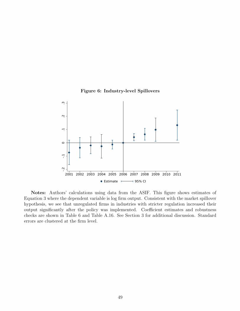
Figure 6: Industry-level Spillovers

-.2-.1

0.1

.2.3

2001 2002 2003 2004 2005 2006 2007 2008 2009 2010 2011

Estimate 95% CI

Notes: Authors’ calculations using data from the ASIF. This figure shows estimates ofEquation 3 where the dependent variable is log firm output. Consistent with the market spilloverhypothesis, we see that unregulated firms in industries with stricter regulation increased theiroutput significantly after the policy was implemented. Coefficient estimates and robustnesschecks are shown in Table 6 and Table A.16. See Section 3 for additional discussion. Standarderrors are clustered at the firm level.

49

Figure 7: Structural Model Fit and Out-of-Sample Validation

A. Moments: Data vs. Model

Share of Firms Share of Output Relative Output

0.2

.4.6

.8M

omen

t Val

ue

<1 5-20 20-100 100+ 5-20 20-100 100+ 1st-2nd 2nd-3rd

Model Data

B. Out-of-Sample Validation: Difference-in-Differences Effects of the Program

OutputRegulated Firms

Related Firms

Market Spillover

Within-Conglomerate

InputsRegulated Firms

Related Firms

Energy EfficiencyRegulated Firms

Related Firms

-50 -40 -30 -20 -10 0 10 20 30 40 50Estimate vs. Model Prediction

Model Prediction 95% CI of Estimate

Notes: This figure shows the model fitting for both the firm size distribution prior to thepolicy and the firm response after the policy. Panel A plots the size distribution of firms predictedby our model in blue bars and the size distribution calculated from the ASIF and economic censusof 2004 in red bars. It shows that our model fits the data well for both the observed firm sizedistribution and the concentration of output prior to the regulation. Panel B plots the firmresponse predicted by the model in red squares and the firm response obtained from our previousdifference-in-differences estimates in blue diamonds. The blue lines span the 95% confidenceinterval for our difference-in-differences estimates. This graph shows that our model does a goodjob of fitting the output, input, and efficiency response of firms, with almost all model-predictedvalues lying within the 95% confidence intervals. See Section 5.2 for additional discussion.

50

Figure 8: Within-Conglomerate Difference-in-Differences

-.6-.3

0.3

.6

2001 2002 2003 2004 2005 2006 2007 2008 2009 2010 2011

Estimate 95% CI

Notes: Authors’ calculations using data from the ASIF. This figure plots the output changeof regulated firms relative to their (same 4-digit industry) related firms within the same con-glomerate. We see a strong and persistent output reallocation following the regulation fromregulated firms to their related firms. Point estimates are displayed in Table 9. See Section 5.3for additional discussion. Conglomerate-by-year fixed effects are included, and standard errorsare clustered at the conglomerate level.

51

Figure 9: Model-Based Estimates of the Shadow Costs of Regulation

A. Shadow Costs of Alternative Regulations

Regulation Threshold

Conglomerate RegulationEnergy Tax

Top 1,000 Program

No Spillover

No Conglomerate Spillover

02.

55

7.5

1012

.515

17.5

20

Shad

ow C

ost o

f Reg

ulat

ion

λ(φ)

0 10 20 30 40 50Conglomerate Productivity

φ

B. Size Distortions in Top 1,000 Program

Conglomerate Size Thresholds

8.67

8.67

58.

688.

685

8.69

8.69

58.

7

Shad

ow C

ost o

f Reg

ulat

ion

λ(φ)

10 20 30 40 50Conglomerate Productivity

φ

Notes: This figure shows the implied shadow cost of different regulations estimated by ourmodel. Panel A plots the shadow cost of our baseline regulation (the Top 1,000 Energy SavingProgram) with the blue line, the shadow cost of the counterfactual in which both conglomeratespillovers and market spillovers are shut down with the gray line, the shadow cost of the coun-terfactual in which only conglomerate spillovers are shut down with the yellow line, the shadowcost of regulating conglomerates with the same energy saving amount with the green line, andthe shadow cost of imposing an energy tax with the same energy saving amount with the dashedred line. For each scenario, we solve the model and calculate the corresponding shadow cost. SeeAppendix E for the equilibrium conditions under these alternative regulations. We can see thatboth market spillovers and conglomerate spillovers lower the shadow cost substantially, whileregulating conglomerates and imposing an energy tax can further lower the shadow cost by over40% with the same amount of energy saving. Panel B zooms in to show the shadow cost un-der our baseline regulation. We see that shadow costs are no longer constant among differentconglomerates as in Panel A. Conglomerates with more firms have a slightly lower shadow cost,while conglomerates with the same number of firms have the same shadow cost. See Section 6.1and Section 6.2 for additional discussion.

52

Figure 10: Welfare Effects of Alternative Regulations

A. Changes to Top 1,000 Program

SCC=$51

SCC=$125

SCC=$160

SCC=$210

Top 1,000→20%

30%

5%

56%

60%

50%-6

-4-2

0

Wel

fare

Cos

t of P

rice

Incr

ease

-ln(P

/P* )

0 2 4 6Reduction in Energy Use

ln(E/E*)

Varying RegulationThreshold φ∼

Varying RegulationIntensity ξ

B. Alternative Regulations

SCC=$160→

Top 1,000→

3.96→ ←4.36

Universal←Energy Tax

SCC=$151

-6-4

-20

Wel

fare

Cos

t of P

rice

Incr

ease

-ln(P

/P* )

0 2 4 6Reduction in Energy Use

ln(E/E*)

Conglomerate-levelRegulation

Size-dependentEnergy Tax

Notes: This figure shows the welfare effects of different regulations measured by the trade-off between reductions in energy use and the welfare cost of price increases. Panel A shows thewelfare effects of the Top 1,000 program. The black lines are indifference curves for different SSCs.The red diamond shows that the Top 1,000 program led to an aggregate energy consumptionreduction of close to 4% and a price level increase of about 3.5%, which can be rationalized withan SSC=$160. The navy line indicates that expanding or contracting policy coverage to coverbetween 50% and 60% of an industry’s energy use does not change the fundamental trade-offbetween reductions in energy consumption and price increases. The crimson line indicates thatincreasing the input reduction quota from 5% to 30% makes this trade-off slightly worse. SeeSection 6.1 for additional discussion. Panel B shows the welfare effects under alternative typesof regulations. Regulating conglomerates and imposing a size-dependent energy tax show asimilar trade-off at an SSC=$152, which is a better performance than that of the original policy.A universal energy tax performs even better, with SSC=$151. See Section 6.2 for additionaldiscussion.

53

Figure 11: Welfare Effects: Robustness

A. Endogenous Energy Efficiency

Baseline→

SCC=$160γ=∞

SCC=$129γ=12.8

SCC=$112γ=7.4

11.6%10.4%

-6-4

-20

Wel

fare

Cos

t of P

rice

Incr

ease

-ln(P

/P* )

0 2 4 6 8 10 12Reduction in Energy Use

ln(E/E*)

C. Alternative Parameters

SCC=$165→SCC=$160→

←SCC=$154

α=0.95α=0.85

ρC=0.9

-6-4

-20

Wel

fare

Cos

t of P

rice

Incr

ease

-ln(P

/P* )

0 2 4 6Reduction in Energy Use

ln(E/E*)

Baseline α=0.9, ρ=0.75 Vary ρ∈0.7,0.9 Vary α∈0.85,0.95 ρC=0.9

B. Heterogeneous Energy Efficiency

Baseline→νR=0.8

νR=0.8νO=0.8

νR=1.2

νR=1.2νO=1.2

SCC=$160

SCC=$191SCC=$196

SCC=$135

SCC=$133

-6-4

-20

Wel

fare

Cos

t of P

rice

Incr

ease

-ln(P

/P* )

0 2 4 6Reduction in Energy Use

ln(E/E*)

Notes: This figure shows the robustness of the welfare effects ofthe Top 1,000 program. The black lines plot indifference curvesfor the baseline value of SCC=$160, and the light gray lines plotvalues of the SCC according to different extensions. Panel Ashows the effects under different values of the parameter γ, whichdetermines the cost of improving energy efficiency. See Section 7.1for details. Panel B shows the effects when we assume preexistingdifferences in energy efficiency. νR > 1 denotes that related firmsare more energy efficient than Top 1,000 firms, while νO < 1denotes that unregulated and unrelated firms are less efficientthan Top 1,000 firms and vice versa. See Section 7.2 for details.Panel C shows the effects when we assume different values ofthe calibrated parameters. Blue triangles hold α = 0.9 and varyρ ∈ 0.7, 0.9, while green circles hold ρ = 0.75 and vary α ∈0.85, 0.98. See Section 7.3 for details. The black square in PanelC plots the effects when we assume that the outputs of firms ina conglomerate are imperfect substitutes (i.e., ρc = 0.9). SeeSection 7.4 for details. Across these wide-ranging assumptions,the SCC that rationalizes the Top 1,000 program lies between$112 and $196.

54

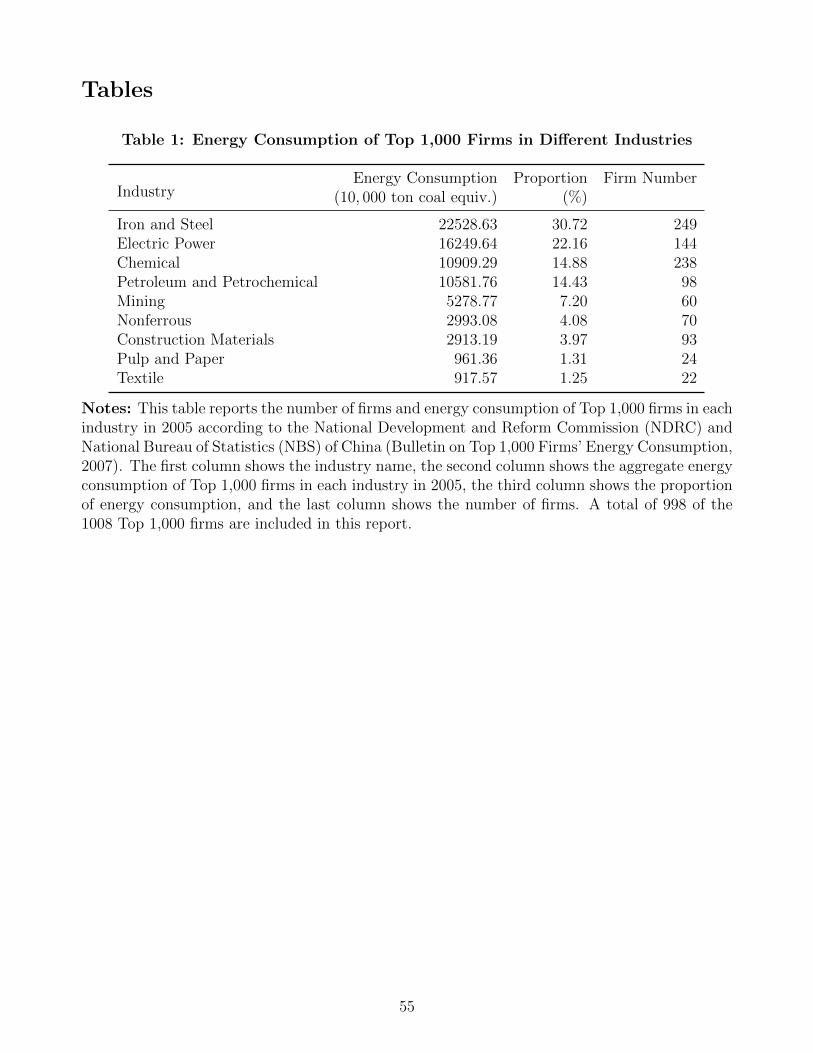
Tables

Table 1: Energy Consumption of Top 1,000 Firms in Different Industries

IndustryEnergy Consumption Proportion Firm Number

(10, 000 ton coal equiv.) (%)

Iron and Steel 22528.63 30.72 249Electric Power 16249.64 22.16 144Chemical 10909.29 14.88 238Petroleum and Petrochemical 10581.76 14.43 98Mining 5278.77 7.20 60Nonferrous 2993.08 4.08 70Construction Materials 2913.19 3.97 93Pulp and Paper 961.36 1.31 24Textile 917.57 1.25 22

Notes: This table reports the number of firms and energy consumption of Top 1,000 firms in eachindustry in 2005 according to the National Development and Reform Commission (NDRC) andNational Bureau of Statistics (NBS) of China (Bulletin on Top 1,000 Firms’ Energy Consumption,2007). The first column shows the industry name, the second column shows the aggregate energyconsumption of Top 1,000 firms in each industry in 2005, the third column shows the proportionof energy consumption, and the last column shows the number of firms. A total of 998 of the1008 Top 1,000 firms are included in this report.

55

Table 2: Summary Statistics

A. Firm-level Data

Source VariablesTop 1,000 Top 10,000

(Excluding Top 1,000)

Obs Mean SD Obs Mean SD

ASIF

ln(Output) 8,745 14.15 1.58 81,547 12.18 1.60Soe 8,787 0.31 0.46 81,833 0.09 0.29ROA 8,564 0.05 0.10 79,944 0.08 0.16Age 8,777 23.03 20.32 81,721 12.55 13.67Export 8,789 0.34 0.47 81,845 0.26 0.44

CESD

ln(Energy) 3,419 12.37 1.48 20,207 9.84 1.58ln(Coal) 3,419 12.41 1.47 20,207 9.91 1.59ln(Output) 3,381 13.69 1.66 20,076 11.26 1.58ln(Efficiency) 3,381 1.31 1.45 20,076 1.42 1.71

B. Conglomerate Networks: Related Parties

DatasetsTwo Levels Six Levels

25% 20% 51% 20%

CARD 46,178 50,846 30,096 77,783CARD&ASIF 7,329 7,907 5,061 9,832CARD&ASIF (same 2-digit industry) 3,992 4,137 2,941 4,800CARD&ASIF (same 4-digit industry) 2,466 2,514 1,963 2,827

Notes: This table reports summary statistics for Top 1,000 firms, Top 10,000 firms, and theconglomerate networks of Top 1,000 firms. Panel A shows the mean characteristics and firmcounts with nonmissing data from the ASIF and CESD for Top 1,000 and Top 10,000 firms.We exclude related firms from the same 4-digit industry as Top 10,000 firms for both datasets.Additionally, for the CESD data, we exclude all industries whose electricity consumption accountsfor more than 30% of total industry energy consumption. See Section 1.2 for a detailed datadescription and the cleaning procedure. Panel B shows the total number of related firms thatTop 1,000 firms have under different definitions of related parties. With 2 levels and a 25%ownership requirement, Top 1,000 firms have 3,992 related firms in the same 2-digit industry inthe ASIF and 2,466 related firms in the same 4-digit industry in the ASIF. See Section 1.3 foradditional discussion.

56

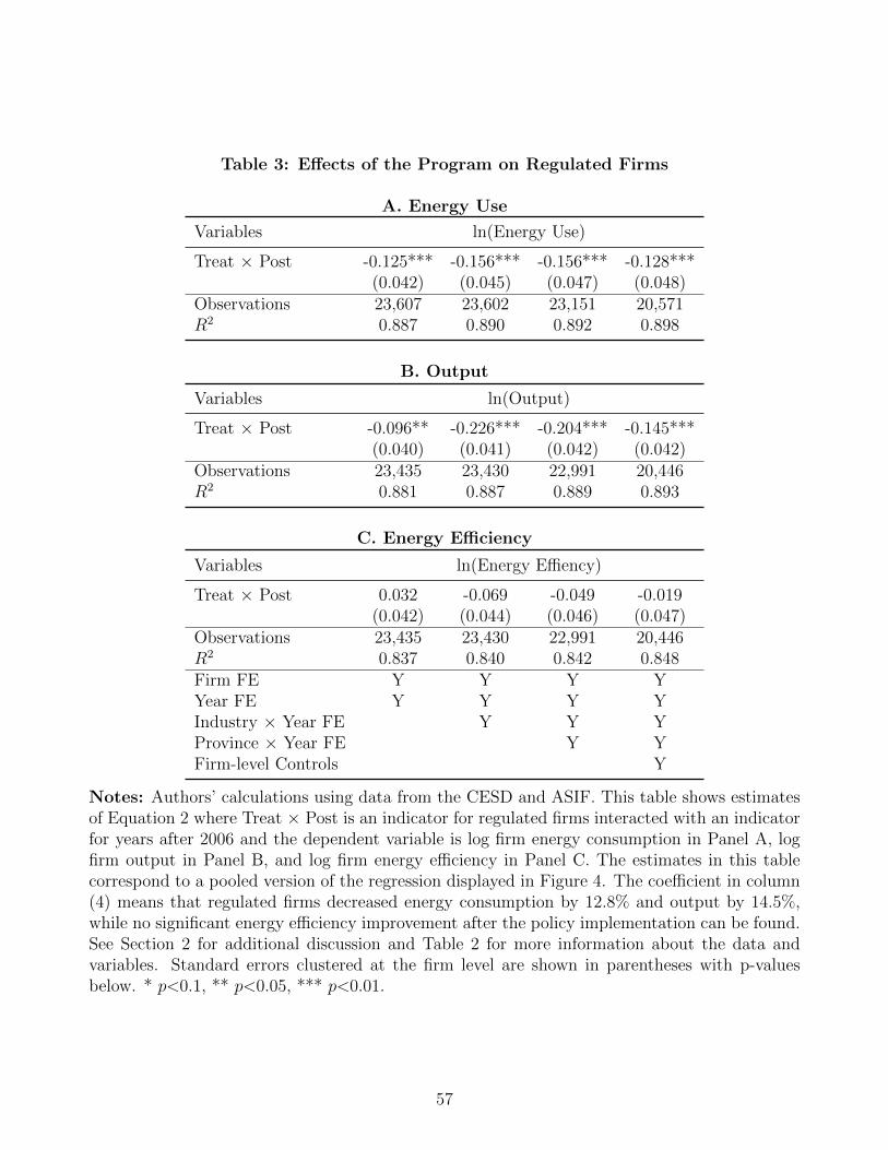
Table 3: Effects of the Program on Regulated Firms

A. Energy Use

Variables ln(Energy Use)

Treat × Post -0.125*** -0.156*** -0.156*** -0.128***(0.042) (0.045) (0.047) (0.048)

Observations 23,607 23,602 23,151 20,571R2 0.887 0.890 0.892 0.898

B. Output

Variables ln(Output)

Treat × Post -0.096** -0.226*** -0.204*** -0.145***(0.040) (0.041) (0.042) (0.042)

Observations 23,435 23,430 22,991 20,446R2 0.881 0.887 0.889 0.893

C. Energy Efficiency

Variables ln(Energy Effiency)

Treat × Post 0.032 -0.069 -0.049 -0.019(0.042) (0.044) (0.046) (0.047)

Observations 23,435 23,430 22,991 20,446R2 0.837 0.840 0.842 0.848Firm FE Y Y Y YYear FE Y Y Y YIndustry × Year FE Y Y YProvince × Year FE Y YFirm-level Controls Y

Notes: Authors’ calculations using data from the CESD and ASIF. This table shows estimatesof Equation 2 where Treat × Post is an indicator for regulated firms interacted with an indicatorfor years after 2006 and the dependent variable is log firm energy consumption in Panel A, logfirm output in Panel B, and log firm energy efficiency in Panel C. The estimates in this tablecorrespond to a pooled version of the regression displayed in Figure 4. The coefficient in column(4) means that regulated firms decreased energy consumption by 12.8% and output by 14.5%,while no significant energy efficiency improvement after the policy implementation can be found.See Section 2 for additional discussion and Table 2 for more information about the data andvariables. Standard errors clustered at the firm level are shown in parentheses with p-valuesbelow. * p<0.1, ** p<0.05, *** p<0.01.

57

Table 4: Spillover Effects on the Output of Related Firms

A. Output

Variables ln(Output)

Related × Post 0.152*** 0.147*** 0.118*** 0.127***(0.037) (0.037) (0.037) (0.035)

Observations 18,423 18,420 18,418 17,905R2 0.865 0.873 0.881 0.889

B. Placebo Test on Output

Variables ln(Output)

Related × Post -0.026 -0.025 -0.015 -0.003(0.040) (0.039) (0.039) (0.038)

Observations 8,923 8,921 8,905 8,730R2 0.898 0.903 0.911 0.919

C. Heterogeneous Effects on Output by Firm Size

Variables ln(Output)

Related × Post(0%-30%) 0.104* 0.109** 0.048 0.078(0.054) (0.052) (0.052) (0.051)

Related × Post(30%-60%) 0.130*** 0.123*** 0.096** 0.111**(0.047) (0.045) (0.046) (0.043)

Related × Post(60%-100%) 0.164*** 0.156*** 0.161*** 0.161***(0.045) (0.044) (0.043) (0.040)

Observations 17,691 17,691 17,689 17,212R2 0.892 0.900 0.907 0.915Firm FE Y Y Y YYear FE Y Y Y YIndustry × Year FE Y Y YProvince × Year FE Y YFirm-level Controls Y

Notes: Authors’ calculations using data from the ASIF. This table shows estimates of Equation2 where Related × Post is an indicator for related firms interacted with an indicator for yearsafter 2006 and the dependent variable is log firm output. The estimates in Panel A correspondto a pooled version of the regression displayed in Panel A of Figure 5. It shows that related firmsin the same 4-digit industries increased output by 11.8%–15.2% after the policy implementation.The estimates in Panel B correspond to a pooled version of the regression displayed in PanelB of Figure 5 and show that related firms outside the 4-digit industry of regulated firms (butstill in the same 2-digit industry) were not significantly affected by the policy. Panel C showsestimates of heterogeneous spillover effects by terciles of firm size. We can see that the relatedspillovers are greater for larger related firms. See Section 3 for additional discussion. The resultsof robustness checks with additional matching methods are shown in Table A.9. Standard errorsclustered at the firm level are shown in parentheses with p-values below. * p<0.1, ** p<0.05,*** p<0.01.

58

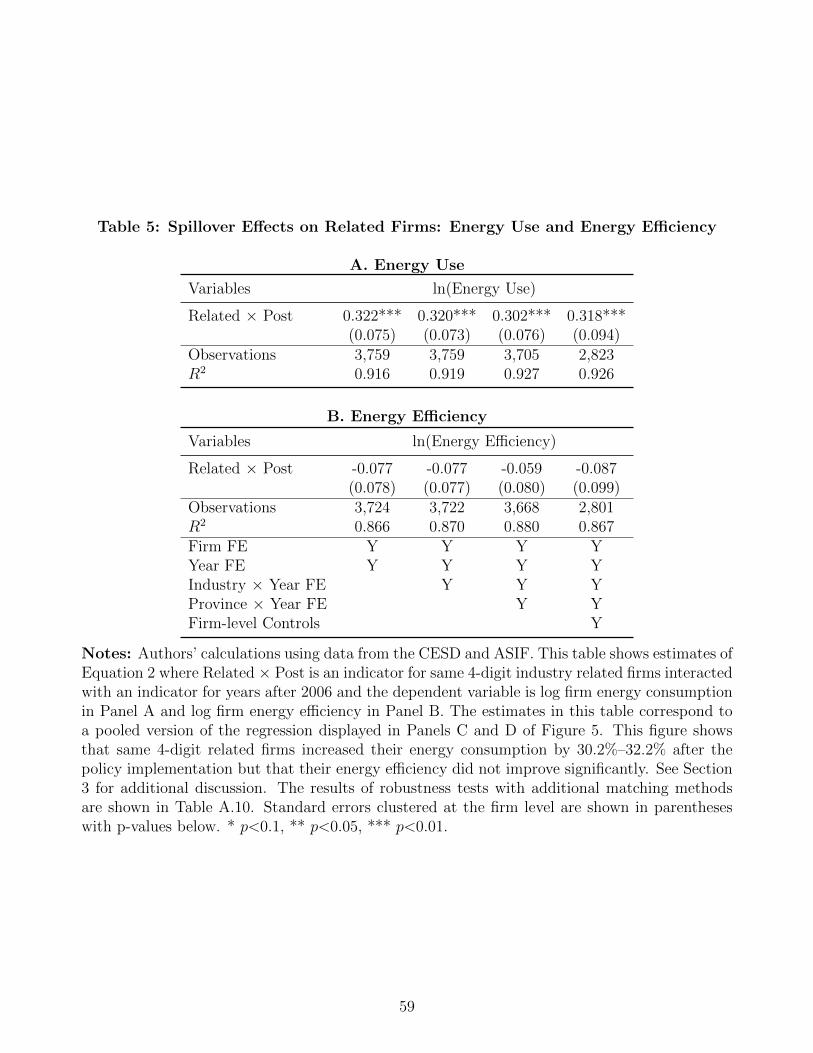
Table 5: Spillover Effects on Related Firms: Energy Use and Energy Efficiency

A. Energy Use

Variables ln(Energy Use)

Related × Post 0.322*** 0.320*** 0.302*** 0.318***(0.075) (0.073) (0.076) (0.094)

Observations 3,759 3,759 3,705 2,823R2 0.916 0.919 0.927 0.926

B. Energy Efficiency

Variables ln(Energy Efficiency)

Related × Post -0.077 -0.077 -0.059 -0.087(0.078) (0.077) (0.080) (0.099)

Observations 3,724 3,722 3,668 2,801R2 0.866 0.870 0.880 0.867Firm FE Y Y Y YYear FE Y Y Y YIndustry × Year FE Y Y YProvince × Year FE Y YFirm-level Controls Y

Notes: Authors’ calculations using data from the CESD and ASIF. This table shows estimates ofEquation 2 where Related × Post is an indicator for same 4-digit industry related firms interactedwith an indicator for years after 2006 and the dependent variable is log firm energy consumptionin Panel A and log firm energy efficiency in Panel B. The estimates in this table correspond toa pooled version of the regression displayed in Panels C and D of Figure 5. This figure showsthat same 4-digit related firms increased their energy consumption by 30.2%–32.2% after thepolicy implementation but that their energy efficiency did not improve significantly. See Section3 for additional discussion. The results of robustness tests with additional matching methodsare shown in Table A.10. Standard errors clustered at the firm level are shown in parentheseswith p-values below. * p<0.1, ** p<0.05, *** p<0.01.

59

Table 6: Industry-level Spillovers

Variables ln(Output)All Sample Energy-Intensive Industries

Spillover × Post 0.081*** 0.073*** 0.083*** 0.084**(0.022) (0.019) (0.023) (0.027)

Observations 2,557,940 2,557,940 843,313 843,313R2 0.840 0.856 0.831 0.848Firm FE Y Y Y YYear FE Y Y Y YIndustry-level Controls Y Y Y YFirm-level Controls Y Y

Notes: Authors’ calculations using data from the ASIF. This table shows estimates of Equation3 where Spillover × Post is an indicator for industry-level exposure to the Top 1,000 programinteracted with an indicator for years after 2006 and the dependent variable is log firm output.Exposure to Top 1,000 program is defined as the proportion of total energy saving targets of Top1,000 firms relative to the total energy consumption in 2004 for each industry. The estimates inthis table correspond to a pooled version of the regression displayed in Figure 6. The results showthat the average market-level spillover led to a 7.3%–8.4% increase in the output of unregulatedfirms. See Section 3 for additional discussion. Standard errors clustered at the firm level areshown in parentheses with p-values below. * p<0.1, ** p<0.05, *** p<0.01.

Table 7: Structural Model Parameters

Parameter Value Target

1. Fixed ValuesElasticity of substitution σ = 1

1−ρ 4.00 Melitz and Redding (2015)

Returns to scale α 0.90 Burnside et al. (1995)Returns to scale (Labor Share) αl 0.80 Cost share of variable inputs2. Method of MomentsEfficiency depreciation δ 0.900 Within-conglomerate distribution

(0.003)Dispersion of ln-ability φ σm 1.239 Firm size distribution

(0.055)Survival threshold φ1 0.609 Share of small firms

(0.166)3. Policy Parameters

Policy threshold φ 9.29 Energy share of Top 1,000 firmsInput quota 1− ξ 0.20 11th Five Year Plan

Notes: This table summarizes the parameters that we set or estimate to solve the model.Standard errors are calculated using a bootstrapped variance-covariance matrix of data moments.See Section 5.1 for the detailed estimation procedure.

60

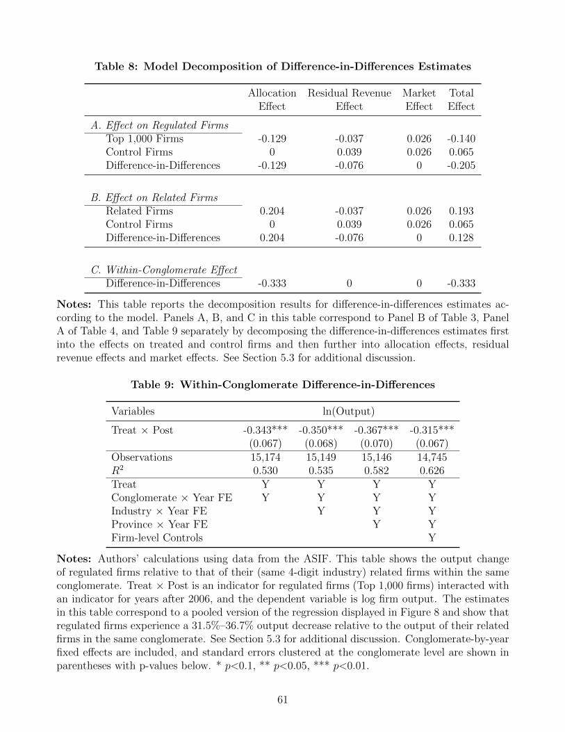
Table 8: Model Decomposition of Difference-in-Differences Estimates

Allocation Residual Revenue Market TotalEffect Effect Effect Effect

A. Effect on Regulated FirmsTop 1,000 Firms -0.129 -0.037 0.026 -0.140Control Firms 0 0.039 0.026 0.065Difference-in-Differences -0.129 -0.076 0 -0.205

B. Effect on Related FirmsRelated Firms 0.204 -0.037 0.026 0.193Control Firms 0 0.039 0.026 0.065Difference-in-Differences 0.204 -0.076 0 0.128

C. Within-Conglomerate EffectDifference-in-Differences -0.333 0 0 -0.333

Notes: This table reports the decomposition results for difference-in-differences estimates ac-cording to the model. Panels A, B, and C in this table correspond to Panel B of Table 3, PanelA of Table 4, and Table 9 separately by decomposing the difference-in-differences estimates firstinto the effects on treated and control firms and then further into allocation effects, residualrevenue effects and market effects. See Section 5.3 for additional discussion.

Table 9: Within-Conglomerate Difference-in-Differences

Variables ln(Output)

Treat × Post -0.343*** -0.350*** -0.367*** -0.315***(0.067) (0.068) (0.070) (0.067)

Observations 15,174 15,149 15,146 14,745R2 0.530 0.535 0.582 0.626Treat Y Y Y YConglomerate × Year FE Y Y Y YIndustry × Year FE Y Y YProvince × Year FE Y YFirm-level Controls Y

Notes: Authors’ calculations using data from the ASIF. This table shows the output changeof regulated firms relative to that of their (same 4-digit industry) related firms within the sameconglomerate. Treat × Post is an indicator for regulated firms (Top 1,000 firms) interacted withan indicator for years after 2006, and the dependent variable is log firm output. The estimatesin this table correspond to a pooled version of the regression displayed in Figure 8 and show thatregulated firms experience a 31.5%–36.7% output decrease relative to the output of their relatedfirms in the same conglomerate. See Section 5.3 for additional discussion. Conglomerate-by-yearfixed effects are included, and standard errors clustered at the conglomerate level are shown inparentheses with p-values below. * p<0.1, ** p<0.05, *** p<0.01.

61

Online Appendix: Not For Publication

This appendix contains multiple additional analyses. Appendix A describes in more detail

the data construction. Appendix B shows that our results are robust to accounting for competing

policies in this time period. Appendix C shows that the program did not lead to a significant

shift in production toward locations with higher emissions and population density. Appendix

D provides a detailed derivation of our baseline model. Appendix E describes how we model

alternative regulations. Appendix F examines the effects of the program when we shut down

market and conglomerate-level spillovers. Finally, Appendix G details the extensions of the

model.

A Details of the Data Merge

Table A.2 shows the results of our data construction. We merge the lists of regulated firms using

both firm name and the unique legal identifier. Since the Top 1,000 and Top 10,000 firms are

all large firms, the match rate with the ASIF is very high. We match over 99% of Top 1,000

firms and over 97% of Top 10,000 firms. We also have a fairly good match rate with the CESD,

where we match over 80% of Top 1,000 and over 70% of Top 10,000 firms. Overall, our combined

datasets capture the majority of the economic activity in Top 1,000 and Top 10,000 firms.

B Robustness of Effects on Regulated Firms to

Competing Policies

This appendix explores the robustness of our results to competing polices. Specifically, in the

same time period when the Top 1,000 program was implemented, the Chinese government also

adopted the National Specially Monitored Firms (NSMF) program. This is an environmental

policy targeting over 6,500 firms in China listed as high polluters in 2007 with a selection rule

for firms’ COD, NH+4 , SO2, smoke and industrial dust emissions in 2005. Half of Top 1,000 firms

and 14% of Top 10,000 firms were included on the NSMF list.

We now show that our estimated effects of the Top 1,000 program are not driven by this

competing policy. Consider first the effect of the NSMF program within the group of firms in the

Top 1,000 program. Panel A of Table A.6 reports estimates of a difference-in-differences model of

the effects of the NSMF program and shows that it had little effect on the energy use, output, and

energy efficiency of Top 1,000 firms. We also consider whether the NSMF program impacts our

estimates of the effects of the Top 1,000 program on regulated firms. Panel B reports estimates

of the effects of the Top 1,000 program when we exclude all treated firms included under both

polices. Panel B shows that we obtain results similar to those in our baseline regressions when

62

we leave out the all Top 1,000 firms included under the NSMF program. These findings suggest

that taking the NSMF program into account does not affect our main results.

C Heterogeneous Effects of Spillovers by Local Density

and Pollution

One important concern is that the spillovers that we identify may have shifted the location

of production and of related emissions to more populated areas and areas with higher levels

of preexisting industrial emissions. To address this concern, we first use data on city-level

sulphur dioxide emissions and population density to generate the following measure of exposure:City SO2 Emission×Population

CityArea. We then calculate the difference in this exposure measure between each

pair of regulated and related firms. Next, we split our sample by terciles of this measure. Table

A.20 shows that related firms in places with lower or similar exposure increased their output by

10%, while those in more exposed areas saw larger increases of close to 22%. However, because

a higher share of the output of related firms was concentrated in less exposed areas (58% in

relatively less exposed vs. 28% in relatively more exposed areas), we find similar increases in

production across more and less exposed areas. Overall, the spillover effects of the regulation

did not disproportionately shift production to areas with higher population density or higher

preexisting levels of industrial emissions.

D Model Appendix

This appendix provides detailed model derivations.

D.1 Model Equilibrium

Recall that the conglomerate takes the prices of energy pe, capital r, and the variable input

bundle w as given. Given the Leontief technology, the conglomerate sets li = ei so that the cost

of intermediate inputs is w + pe. Holding the number of affiliates n constant, the conglomerate

maximizes

π(φ, n) = maxlini=1,kini=1

R1−ρP ρ

[n∑i=1

φδi−1kαki lαli

]ρ− (w + pe)

n∑i=1

li − rn∑i=1

ki

.

For a firm i, the first-order conditions for li and ki imply that li = αlαk

r(w+pe)

ki.

Substituting this expression, we can write the profit maximization problem as

π(φ, n) = maxkini=1

R1−ρP ρ

[n∑i=1

φδi−1kαi

(αlαk

r

(w + pe)

)αl]ρ−(α

αkr

) n∑i=1

ki

.

63

Comparing the first-order conditions for k1 and ki, we find that kik1

= δi−11−α . The final result from

Proposition 1 follows since

qi = φδi−1kαi

(αlαk

r

(w + pe)

)αl= φδ

i−11−αkα1

(αlαk

r

(w + pe)

)αl= δ

i−11−α q1.

Using these results, we can write the profit maximization problem in terms of Kn =∑n

i ki.

To do so, we define the conglomerate’s total productivity φ∆n = φ[∑n

i=1(δi−1)1

1−α ]1−α and the

constant Cπ = (1− αρ)[(

ραlw+pe

)αlρ (ραkr

)αkρ] 11−αρ

to obtain

π(φ, n) = maxKn

R1−ρP ρC1−αρ

π

(1− αρ)1−αρ

(ραkr

)−αρ(φ∆n)ρKαρ

n − r(α

αk

)Kn

.

The optimal capital Kn and the firm profits for a conglomerate of size n are then

Kn =R

1−ρ1−αρP

ρ1−αρCπ

(1− αρ)

ραkr

(φ∆n)ρ

1−αρ and π(φ, n) = R1−ρ1−αρP

ρ1−αρCπ (φ∆n)

ρ1−αρ .

The optimal profit given φ is then

π(φ) = maxn

π(φ, n)− rfn = maxn

R1−ρ1−αρP

ρ1−αρCπ × (φ∆n)

ρ1−αρ − rfn.

Solving for indifference points φn yields the result of Proposition 2 and the zero-profit condition

(Equation 7).

We now compute the price level. For given quantities q(φ, n), the price level is given by

P−ρ = R−ρ∫φ1

q(φ, n)ρg(φ)M

1−G(φ1)dφ.

To differentiate from the regulated case below, we use starred variables to denote prices and

quantities in the unregulated case. To derive q∗(φ, n), note from Proposition 1 that Kn = k1∆1

1−αn

and also recall that l1 = αlαk

r(w+pe)

k1. We then have

q∗(φ, n) = ∆1

1−αn q∗1(φ, n)

= ∆1

1−αn φ

(αlαk

r

(w + pe)

)αlk∗1

α

= (φ∆n)1

1−αρ R(1−ρ)α1−αρ P ∗

ρα1−αρ ρ

α1−αρ

[(αl

w + pe

)αl (αkr

)αk] 11−αρ

︸ ︷︷ ︸=CQ

. (D.1)

64

The price level absent the regulation is then

P ∗−ρ = R−ρ∫φ1

((φ∆n)

11−αρ R

(1−ρ)α1−αρ P ∗

ρα1−αρCQ

)ρ g(φ)M

1−G(φ1)dφ

P ∗−ρ

1−αρR(1−α)ρ1−αρ C−ρQ =

∫φ1

(φ∆n)ρ

1−αρg(φ)M

1−G(φ1)dφ.

P ∗−ρ

1−αρR(1−α)ρ1−αρ C−ρQ

1−G(φ1)

M=

∫φ1

(φ∆n)ρ

1−αρ g(φ)dφ

P ∗−ρ

1−αρR(1−α)ρ1−αρ C−ρQ

1−G(φ1)

M=

∑n

∆ρ

1−αρn

φn+1∫φn

(φ)ρ

1−αρ g(φ)dφ

︸ ︷︷ ︸=πn

=∑n

∆ρ

1−αρn πn.

Given the assumption that φ follows a log-normal distribution, we can express

πn =

φn+1∫φn

(φ)ρ

1−αρ g(φ)dφ = exp

σ2

2

[Φ(bn+1 − σ)− Φ(bn − σ)],

where σ = ρ1−αρσφ and bn = ρ

1−αρln(φn)σ

. Note also that Equations 6 and 7 imply that

φn+1 =φ1(

∆ρ

1−ραn+1 −∆

ρ1−ραn

) 1−ραρ

.

Thus, πn depends on φ1; it does not directly depend on equilibrium prices P ∗.

D.2 Response to Top 1,000 Program

The Top 1,000 program limits energy use at the largest firm e1 to a fraction ξ < 1 of the energy

use in the unregulated case e∗1; recall that we use starred variables to denote the optimal choices

in the unregulated case. We assume that the number of firms n and the capital allocations

k∗i ni=1 are quasifixed but that the conglomerate can adjust lini=1.

Regulated Conglomerates

Using the fact that k∗i = k∗1δi−11−α , we can write the profit maximization problem as

maxlin1

R1−ρP ρ

[φ∗

n∑i=1

δ(i−1)(1−αl)

1−α lαli

]ρ− (w + pe)

n∑i=1

li − rn∑i=1

k∗i

subject to l1 ≤ ξl∗1,

where φ∗ = φ(k∗1)αk . The first-order conditions for li (1 ≤ i ≤ n) are then

∂π

∂li= R1−ρP ρ︸ ︷︷ ︸

Market Demand

ρ

[φ∗

n∑i=1

δ(i−1)(1−αl)

1−α lαli

]ρ−1

︸ ︷︷ ︸Residual Revenue

φ∗δ(i−1)(1−αl)

1−α αl(li)αl−1︸ ︷︷ ︸

Marginal Product

= w + pe + λ(φ)I[i = 1]︸ ︷︷ ︸Shadow Cost

of Regulation

.

65

These conditions yield the results in Proposition 3.

We now show that given n, λ(φ) does not depend on φ. To do so, we note that an implication

of Proposition 3 is that we can write total conglomerate production under the regulation as

q(φ, n) =n∑i

qi(φ, n) = q1(φ, n)

[1 +

n∑i>1

δi−11−α

[1 +

λ(φ)

w + pe

] αl1−αl

].

In contrast, recall from Proposition 1 that in the unregulated case total conglomerate output is

q∗(φ, n) =n∑i

q∗i (φ, n) = q∗1(φ, n)n∑i

δi−11−α .

To connect these expressions, note that since k∗1 is fixed and l1 = ξl∗1, we have that

q1(φ, n) = φ(k∗1)αk(l1)αl = φ(k∗1)αk(l∗1)αlξαl = q∗1(φ, n)ξαl .

Together, the last three expression imply that

q(φ, n) = q∗(φ, n)ξαl

[1 +

n∑i>1

δi−11−α

[1 + λ(φ)

w+pe

] αl1−αl

]n∑i

δi−11−α

= q∗(φ, n)

ξαl 1 + (∆1

1−αn − 1)

[1 + λ(φ)

w+pe

] αl1−αl

∆1

1−αn

︸ ︷︷ ︸

=ξq,n

,

(D.2)

where ξq,n captures the impact of the regulation on conglomerate output.

Using this expression and the fact that l1 = ξl∗1, we can rewrite the first-order condition for

l1 in terms of the capital and labor choices in the unregulated case:

R1−ρP ∗ρρ

[φ

n∑i=1

δi−11−α (k∗i )

αk(l∗i )αl

]ρ−1

× φαl(k∗1)αk(l∗1)αl−1

︸ ︷︷ ︸FOC Unregulated Case

×(ξ)αl−1

(P

P ∗

)ρ ξαl 1 + (∆1

1−αn − 1)

[1 + λ(φ)

w+pe

] αl1−αl

∆1

1−αn

ρ−1

= w + pe + λ(φ),

where PP ∗

is the equilibrium change in the industry-level price. Using the fact that the first-order

condition in the unregulated case equals w + pe, we have

(ξ)αl−1

(P

P ∗

)ρ ξαl 1 + (∆1

1−αn − 1)

[1 + λ(φ)

w+pe

] αl1−αl

∆1

1−αn

(ρ−1)

= 1 +λ(φ)

w + pe. (D.3)

66

This expression shows that conditional on n, the shadow cost does not depend on φ, and so we

now write λn. The expression above is equivalent to[1 +

λnw + pe

] 11−ρ[

1 + (∆1

1−αn − 1)

[1 +

λnw + pe

] αl1−αl

]=

(P

P ∗

) ρ1−ρ

ξ−(1−αlρ)

1−ρ ∆1

1−αn . (D.4)

This expression does not have a general closed-form solution. Consider, however, the special

case where 11−ρ = αl

1−αl.58 In this special case, we can write this expression as

(∆1

1−αn − 1)x2 + x−

(P

P ∗

) ρ1−ρ

ξ−(1−αlρ)

1−ρ ∆1

1−αn = 0,

where x =[1 + λn

w+pe

] 11−ρ

=[1 + λn

w+pe

] αl1−αl , which allows us to solve for λn using the quadratic

formula. Focusing on the positive root implies

1 +λn

w + pe=

−1 +

√1 + 4(∆

11−αn − 1)

(PP ∗

) ρ1−ρ ξ

−(1−αlρ)1−ρ ∆

11−αn

2(∆1

1−αn − 1)

1−ρ

.

Note that λn depends on the equilibrium price P in both the expression above and in Equation

D.4. In this case, we also have

ξq,n = ξαl1 +

√1 + 4(∆

11−αn − 1)

(PP ∗

) ρ1−ρ ξ

−(1−αlρ)1−ρ ∆

11−αn

2∆1

1−αn

.

Unregulated Conglomerates

Unregulated conglomerates are affected by the policy through the price adjustment in the product

market. The first-order conditions for li (1 ≤ i ≤ n) are then

∂π

∂li= R1−ρP ρρ

[φ∗

n∑i=1

δ(i−1)(1−αl)

1−α lαli

]ρ−1

φ∗δ(i−1)(1−αl)

1−α αl(li)αl−1 = w + pe.

Since these firms do not face a shadow cost, the conditions of Proposition 1 continue to hold.

Using these results to solve for l1, we obtain

l1 =

R1−ρP ρρ[φ(k∗1)αk ]ρ∆ρ−11−αn αl

w + pe

11−αlρ

.

This further implies that

l1 = l∗1

(P

P ∗

) ρ1−αlρ

(D.5)

58While this is a knife-edge case, it holds in the empirically relevant case of ρ = .75 and αl = 0.8, so that1

1−ρ = αl1−αl = 4.

67

and both

q1(φ, n) = q∗1(φ, n)

(P

P ∗

) αlρ

1−αlρ

and q(φ, n) = q∗(φ, n)

(P

P ∗

) αlρ

1−αlρ

. (D.6)

D.2.1 Product Market Equilibrium

We now derive the equilibrium price under the Top 1,000 program. Recall that only conglomer-

ates with φ ≥ φ have a regulated firm. Under the definition of ξq,n in Equation D.2 for regulated

firms and Equation D.6 for unregulated firms, the price level under the regulation is then

P−ρ = R−ρ∫ φ

φ1

((P

P ∗

) αlρ

1−αlρ

(φ∆n)1

1−αρ R(1−ρ)α1−αρ P ∗

ρα1−αρCQ

)ρ

g(φ)M

1−G(φ1)dφ

+ R−ρ∫φ

(ξq,n (φ∆n)

11−αρ R

(1−ρ)α1−αρ P ∗

ρα1−αρCQ

)ρ g(φ)M

1−G(φ1)dφ.

As in the case of the unregulated equilibrium, we use πn to denote the output of conglomerates

with n affiliates. However, the regulation threshold φ in general does not line up with the size

thresholds φn that define πn. Let n denote the smallest firm size for regulated conglomerates.

We split πn into π1 and π2 as follows:

π1 =

φ∫φn

(φ)ρ

1−αρ g(φ)dφ and π2 =

φn+1∫φ

(φ)ρ

1−αρ g(φ)dφ.

We can then manipulate the expression for the equilibrium price as follows:

P−ρP ∗−ρ2α1−αρR

(1−α)ρ1−αρ C−ρQ

1−G(φ1)

M=

(P

P ∗

) αlρ2

1−αlρ(n−1∑n=1

∆ρ

1−αρn πn + ∆

ρ1−αρn π1

)+ ξρq,n∆

ρ1−αρn π2 +

∑n=n+1

ξρq,n∆ρ

1−αρn πn.

Note that this equation holds in the case absent the regulation if we set ξq,n = 1 and P = P ∗.

Let sφ =∆

ρ1−αρn π2+

∑n=n+1

∆ρ

1−αρn πn

∑n

∆ρ

1−αρn πn

be the output share of the Top 1,000 conglomerates prior to the

regulation. Additionally, we introduce the notation:

Ee[xn

∣∣∣φ > φ]

= xn

∆ρ

1−αρn π2

∆ρ

1−αρn π2 +

∑n=n+1

∆ρ

1−αρn πn

+∑n=n+1

xn

∆ρ

1−αρn πn

∆ρ

1−αρn π2 +

∑n=n+1

∆ρ

1−αρn πn

to denote the average of a size-dependent variable xn conditional on being part of the Top 1,000

program with respect to the distribution of energy use in the unregulated equilibrium.

68

Assuming that the regulation does not impact r and w, taking the ratio of price levels before

and after the regulation, we obtain

(P

P ∗

)−ρ= (1− sφ)

(P

P ∗

) αlρ2

1−αlρ

+ sφEe[ξρq,n

∣∣∣φ > φ]. (D.7)

Equations D.4 and D.7 jointly determine the shadow costs of the regulation λnn≥n and the

increase in the price level PP ∗

.

D.2.2 Characterizing Energy Use

Recall that the energy use in firm 1 before the regulation is

e∗1(φ, n) = l∗1(φ, n) =

(αlαk

r

(w + pe)

)k∗1(φ, n) =

(αlαk

r

(w + pe)

)(K∗n

∆1

1−αn

).

The energy use for the conglomerate before the regulation is then

e∗(φ, n) =

(αlαk

r

(w + pe)

)K∗n

= (φ∆n)ρ

1−αρ R1−ρ1−αρP ∗

ρ1−αρ ρ

11−αρ

[(αl

w + pe

)1−αkρ (αkr

)αkρ] 11−αρ

︸ ︷︷ ︸=CE

. (D.8)

The total energy use prior to the regulation is then

E∗ =

∫φ1

e∗(φ, n)g(φ)M

1−G(φ1)dφ

= R1−ρ1−αρP ∗

ρ1−αρ

CEM

1−G(φ1)

∑n

(∆n)ρ

1−αρ πn.

Regulated Conglomerates

We now characterize the change in energy use for regulated conglomerates. The fact that ei = li

and the results of Proposition 1 imply that the energy use for an unregulated conglomerate is

e∗(φ, n) =∑i

e∗i (φ, n) = e∗1(φ, n)n∑i

δi−11−α .

Proposition 3 implies that the energy use for a regulated conglomerate is

e(φ, n) =∑i

ei(φ, n) = e1(φ, n)

[1 +

n∑i>1

δi−11−α

[1 +

λnw + pe

] 11−αl

].

69

Using the fact that e1 = ξe∗1, we then have

e(φ, n) = e∗(φ, n)

ξ

[1 +

n∑i>1

δi−11−α

[1 + λn

w+pe

] 11−αl

]n∑i

δi−11−α︸ ︷︷ ︸

=ξe,n

,

where ξe,n captures the effect of the regulation on the energy use of a regulated conglomerate.

Unregulated Conglomerates

Proposition 1 and Equation D.5 imply that for unregulated conglomerates,

e1(φ, n) = e∗1(φ, n)

(P

P ∗

) ρ1−αlρ

and additionally that

e(φ, n) = e∗(φ, n)

(P

P ∗

) ρ1−αlρ

.

Aggregate Change in Energy

Putting the above together, total energy use after the regulation is now

E =

∫φ1

e(φ, n)g(φ)M

1−G(φ1)dφ =

φ∫φ1

(P

P ∗

) ρ1−αlρ

e∗(φ, n)g(φ)M

1−G(φ1)dφ+

∫φ

ξe,ne∗(φ, n)

g(φ)M

1−G(φ1)dφ

= R1−ρ1−αρP ∗

ρ1−αρ

CEM

1−G(φ1)

[(n−1∑n=1

∆ρ

1−αρn πn + ∆

ρ1−αρn π1

)(P

P ∗

) ρ1−αlρ

+ ξe,n∆ρ

1−αρn π2 +

∑n=n+1

ξe,n∆ρ

1−αρn πn

].

This implies that

E

E∗=

(n−1∑n=1

∆ρ

1−αρn πn + ∆

ρ1−αρn π1

)(PP ∗

) ρ1−αlρ + ξe,n∆

ρ1−αρn π2 +

∑n=n+1

ξe,n∆ρ

1−αρn πn∑

n

(∆n)ρ

1−αρ πn

= (1− sφ)

(P

P ∗

) ρ1−αlρ

+ sφEe[ξe,n

∣∣∣φ > φ]. (D.9)

Equation D.9—along with the equilibrium price increase and shadow costs determined by

Equations D.4 and D.7—allows us to compute the effect of the regulation on welfare.

70

D.2.3 Solving the New Equilibrium Using Reduced-Form Estimates

In Section 6, we present the full solution to the model using the derivations above. This appendix

shows that we can also solve for an approximation of the equilibrium based on our reduced-form

estimates. To do so, we make the assumption that λ and ∆ are constant for regulated firms.

Taking the value of λ implied by our reduced-form estimate of 8.95% and ∆1

1−α = 1.6 (which

approximates the value for n = 6), we use Proposition 4 to compute the production distortion

ξq = 0.9648. Equation 14 delivers the equilibrium price change: ln(PP ∗

)= 4.2%. We then compute

that regulated conglomerates lower their energy use by 5.6%. Finally, we use these numbers to

implement Equation 15, where we find that ln(EE∗

)= −3.65%. The advantage of this calculation

is that it relies on only a handful of calibrated parameter values and the result of the within-

conglomerate difference-in-differences estimation. In particular, this calculation does not rely on

distributional assumptions for G(φ). It is thus reassuring that we obtain aggregate quantities

close to those in the full model solution.

E Alternative Regulations

Conglomerate-level Regulation

Suppose that instead of regulating the energy use of the top firm, the government restricted the

energy use of all firms in a conglomerate to at most ξ of the energy use at the Top 1,000 firm

plus the energy use at related firms. The regulatory constraint would be

e(φ, n) ≤ ξe,ne∗(φ, n).

Arguments similar to the derivation for Equation D.9 imply that

EC

E∗= (1− sφ)

(PC

P ∗

) ρ1−αlρ

+ sφEe[ξe,n|φ > φ

], (E.1)

where we use the superscript C to denote the case of the conglomerate-level regulation.

Since energy use in all firms contributes equally to the regulatory constraint, this regulation

does not distort the allocation of inputs across related firms; i.e., Proposition 1 continues to hold.

This implies that li = ξe,nl∗i for all firms i in the conglomerate. It further implies that

q(φ, n) = (ξe,n)αl q∗(φ, n).

Arguments similar to the derivation for Equation D.7 imply that

(PC

P ∗

)−ρ= (1− sφ)

(PC

P ∗

) αlρ2

1−αlρ

+ sφEe[

(ξe,n)αlρ|φ > φ]. (E.2)

71

We now derive the shadow cost of this regulation. Substituting li into the first-order condition

for firm 1 implies that

R1−ρP ∗ρρ

[φ

n∑i=1

δi−11−α (k∗i )

αk(l∗i )αl

]ρ−1

× φαl(k∗1)αk(l∗1)αl−1

︸ ︷︷ ︸FOC Unregulated Case

× (ξe,n)αl−1

(PC

P ∗

)ρ[(ξe,n)αl ]

ρ−1= w + pe + λC(φ).

Using the fact that the first-order condition in the unregulated case equals w + pe, we obtain[1 +

λCnw + pe

]=

(PC

P ∗

)ρ(ξe,n)−(1−αlρ) .

Size-dependent Energy Tax

Suppose that the government instituted a per-unit energy tax for all the affiliates of conglomerates

with φ > φ. As in the case above, this policy would not impact the within-conglomerate allocation

of inputs of regulated firms, and Proposition 1 would continue to hold. That is, related firms

would all reduce their energy use by the same proportion. Let λτξ be the tax associated with a

proportional energy reduction use of 1− ξτ . The first-order condition for firm 1 is then

R1−ρP ∗ρρ

[φ

n∑i=1

δi−11−α (k∗i )

αk(l∗i )αl

]ρ−1

× φαl(k∗1)αk(l∗1)αl−1

︸ ︷︷ ︸FOC Unregulated Case

× (ξτ )αl−1

(P τ

P ∗

)ρ[ξαlτ ]ρ−1 = w + pe + λτξ ,

where we use the superscript τ to denote this case. Using the fact that the first-order condition

in the unregulated case equals w + pe, we obtain[1 +

λτξw + pe

]=

(P τ

P ∗

)ρ(ξτ )

−(1−αlρ) .

Since all related firms reduce their energy use by the same proportion, it follows that e(φ, n) =

ξτe∗(φ, n) for regulated firms. Arguments similar to the derivation for Equation D.9 imply that

Eτ

E∗= (1− sφ)

(P τ

P ∗

) ρ1−αlρ

+ sφξτ . (E.3)

Noting that q(φ, n) = ξαlτ q∗(φ, n) then implies that

(P τ

P ∗

)−ρ= (1− sφ)

(P τ

P ∗

) αlρ2

1−αlρ

+ sφ(ξτ )αlρ. (E.4)

72

To make this case comparable to the Top 1,000 regulation, we implement a tax that leads to the

same average energy reduction:[1 +

λτξw + pe

]=

(P τ

P ∗

)ρ (Ee[ξe,n

∣∣∣φ > φ])−(1−αlρ)

;

that is, ξτ = Ee[ξe,n

∣∣∣φ > φ]. Note that the aggregate effects differ to the extent that we obtain

different price responses (and therefore different responses from unregulated firms).

F Inspecting the Effect Mechanisms of the Top 1,000

Regulation

Shutting down Market Leakage

In this case, firms believe that prices do not adjust. The perceived shadow cost is given by the

solution to [1 +

λnw + pe

] 11−ρ[

1 + (∆1

1−αn − 1)

[1 +

λnw + pe

] αl1−αl

]= ξ

−(1−αlρ)1−ρ ∆

11−αn .

We recompute ξe,n and ξq,n based on these shadow costs. Aggregate energy use is then given by

E

E∗= (1− sφ) + sφEe

[ξe,n

∣∣∣φ > φ].

The new price is given by(P

P ∗

)−ρ= (1− sφ) + sφEe

[ξρq,n

∣∣∣φ > φ].

The actual shadow cost follows Equation 14 by incorporating the equilibrium price adjustment.

Shutting down Conglomerate Leakage

In this case, we set e1(φ, n) ≤ ξe∗1(φ, n). We further assume that firms related to regulated firms

do not take into account the reduction in e1(φ, n) but do respond to the market price increase,

so that ei(φ, n) =(PP ∗

) ρ1−αlρ e∗i (φ, n) for i ≥ 2. We then have

e(φ, n) = ξe∗1(φ, n) +∑i=2

e∗i (φ, n)

(P

P ∗

) ρ1−αlρ

= e∗1(φ, n)

(ξ +

(P

P ∗

) ρ1−αlρ

(∆

11−αn − 1

))

= e∗(φ, n)

ξ +(PP ∗

) ρ1−αlρ

(∆

11−αn − 1

)∆

11−αn

.

73

Aggregate energy use is then

E

E∗= (1− sφ)

(P

P ∗

) ρ1−αlρ

+ sφEe

ξ +(PP ∗

) ρ1−αlρ

(∆

11−αn − 1

)∆

11−αn

∣∣∣∣∣∣∣∣φ > φ

.Similarly, the effect on total production is

q(φ, n) = ξαlq∗1(φ, n) +∑i=2

q∗i (φ, n)

(P

P ∗

) αlρ

1−αlρ

= q∗1(φ, n)

(ξαl +

(P

P ∗

) αlρ

1−αlρ(

∆1

1−αn − 1

))

= q∗(φ, n)

ξαl +(PP ∗

) αlρ

1−αlρ

(∆

11−αn − 1

)∆

11−αn

.

Aggregate prices are then

(P

P ∗

)−ρ= (1− sφ)

(P

P ∗

) αlρ2

1−αlρ

+ sφEe

ξ

αl +(PP ∗

) αlρ

1−αlρ

(∆

11−αn − 1

)∆

11−αn

ρ∣∣∣∣∣∣∣∣φ > φ

.We now derive the shadow cost of the regulation for the Top 1,000 firm. Substituting li into

the first-order condition for firm 1 implies that

R1−ρP ∗ρρ

[φ

n∑i=1

δi−11−α (k∗i )

αk(l∗i )αl

]ρ−1

× φαl(k∗1)αk(l∗1)αl−1

︸ ︷︷ ︸FOC Unregulated Case

× (ξ)αl−1

(P

P ∗

)ρ ξαl +

(PP ∗

) αlρ

1−αlρ

(∆

11−αn − 1

)∆

11−αn

ρ−1

= w + pe + λ(φ)

Using the fact that the first-order condition in the unregulated case equals w + pe, we obtain

[1 +

λnw + pe

]=

(P

P ∗

)ρξ−(1−αl)

ξαl +

(PP ∗

) αlρ

1−αlρ

(∆

11−αn − 1

)∆

11−αn

−(1−ρ)

.

Shutting down Both Market and Conglomerate Leakage

Energy use and production at regulated conglomerates is the same as in the case in which only

the conglomerate leakage is shut down. Unregulated firms assume that there will be no price

increase, such that the aggregate energy use is then

E

E∗= (1− sφ) + sφEe

ξ − 1 + ∆1

1−αn

∆1

1−αn

∣∣∣∣∣∣φ > φ

.74

Aggregate prices are then(P

P ∗

)−ρ= (1− sφ) + sφEe

ξαl − 1 + ∆1

1−αn

∆1

1−αn

ρ∣∣∣∣∣∣φ > φ

.The actual shadow cost follows Equation 14 using the following definition of ξq(φ) = ξ−1+∆

11−αn

∆1

1−αn

and the equilibrium price above.

G Model Extensions

G.1 Endogenous Energy Efficiency

Assume that the conglomerate can improve energy efficiency at firm i, νi, by spending lic(νi),

where c′(νi) > 0 and c′′(νi) ≥ 0. The conglomerate’s problem is then

π(φ, n) = maxlini=1,νini=1

R1−ρP ρ

[φ∗

n∑i=1

δ(i−1)(1−αl)

1−α lαli

]ρ−

n∑i=1

li

(w +

peνi

+ c(νi)

),

where we omit the cost of fixed capital. Absent the regulation, the conglomerate sets c′(ν∗)ν∗2 =

pe for all firms, so that Proposition 1 continues to hold.

We assume that c(ν) = νγ

1+γ, where γ ≥ 1, so the effective price of energy is (ν∗)γ. Additionally,

note that the Top 1,000 regulation does not impact the choice of νi for unregulated firms. Using

these results and the fact that νi = liei, we can restate the conglomerate problem as

π(φ, n) = maxlini=1

R1−ρP ρ

[φ∗

n∑i=1

δ(i−1)(1−αl)

1−α lαli

]ρ− (w + (ν∗)γ)

n∑i=1

li −l1[

1

1 + γ

(l1ξe∗1

)γ− (ν∗)γ

],

where we substitute the regulatory constraint into the cost of energy efficiency and abstract away

from the cost of the regulated energy.

Deriving the Shadow Cost of Regulation

The conglomerate’s first-order conditions for li (1 ≤ i ≤ n), i.e., ∂π∂li

, are then

R1−ρP ρρ

[φ∗

n∑i=1

δ(i−1)(1−αl)

1−α lαli

]ρ−1

φ∗δ(i−1)(1−αl)

1−α αl(li)αl−1 = w + (ν∗)γ +

[(l1ξe∗1

)γ− (ν∗)γ

]I[i = 1].

We can write the binding energy use constraint as ξe∗1 = e1 = l1ν1

so that ν1 = l1ξe∗1. It is also useful

to write the share of variable input costs accounted for by energy as se = (ν∗)γ

w+(ν∗)γ. The shadow

cost of the policy as a fraction of variable inputs is then

λ(φ)

w + (ν∗)γ=

1

w + (ν∗)γ

[(l1ξe∗1

)γ− (ν∗)γ

]= se

((ν1

ν∗

)γ− 1).

75

Using these expressions, we can then write the ratios of these first-order conditions between j ≥ 2

and the Top 1,000 firm as

ljl1

= δj−11−α

[1 + se

((ν1

ν∗

)γ− 1)] 1

1−αl = δj−11−α

[1 +

λ(φ)

w + (ν∗)γ

] 11−αl

,

which confirms that the results of Proposition 3 extend to the case of endogenous energy efficiency.

We can then write the first-order condition for the Top 1,000 firm as

R1−ρ(P ∗)ρρ

[φ∗

n∑i=1

δ(i−1)(1−αl)

1−α (l∗i )αl

]ρ−1

φ∗αl(l∗1)αl−1

︸ ︷︷ ︸FOC Unregulated

(P

P ∗

)ρ(G.1)

(ξν1

ν∗

)αl [1 +[1 + λ(φ)

w+(ν∗)γ

] αl1−αl ∑

j>1 δj−11−α

]∑

i δj−11−α︸ ︷︷ ︸

ξνq,n

ρ−1

×(ξν1

ν∗

)αl−1

= (w + (ν∗)γ)

[1 +

λ(φ)

w + (ν∗)γ

].

This equation also defines the relevant decrease in conglomerate-level production ξνq,n, which we

use to solve the new product market equilibrium (cf. Propositions 4–5). Noting that the first-

order condition for the unregulated firm equals w+ (ν∗)γ, we can derive the following expression

[1 +

λ(φ)

w + (ν∗)γ

] 11−ρ[

1 + (∆1

1−αn − 1)

[1 +

λ(φ)

w + (ν∗)γ

] αl1−αl

]=

(P

P ∗

) ρ1−ρ(ξν1

ν∗

)−(1−αlρ)1−ρ

∆1

1−αn . (G.2)

This equation has one difference from Equation D.4. Since conglomerates can avoid the impact

of the regulation by increasing the energy efficiency of the Top 1,000 firm, the effective regulation

is now ξν1ν∗. That is, conglomerates have less of a need to reduce their energy use if they increase

ν1. This also implies that λ(φ) is decreasing in ν1. Similar to Equation D.4, note that in this

equation, the ratio ν1ν∗

is an implicit function of quantities that are common for firms with the

same number of affiliates n. This implies that firms with different values of φ have the same

shadow cost and improvement to energy efficiency as long as they belong to a conglomerate of

the same size. We then write λn and ν1,n to signify the dependence of these variables on n.

Aggregate Energy Use

Prior to the regulation, we have that e∗(φ, n) = l∗(φ,n)ν∗

for both regulated and unregulated

firms. For unregulated firms, we still have e(φ, n) = l(φ,n)ν∗

since these firms do not change their

76

investment in energy efficiency. However, for regulated conglomerates, we have

e(φ, n) =l1ν1,n

+1

ν∗

∑i>1

li =l1ν1,n

(1 +

ν1,n

ν∗(∆

11−αn − 1)

[1 +

λnw + (ν∗)γ

] 11−αl

)

= e1(φ, n)

(1 +

ν1,n

ν∗(∆

11−αn − 1)

[1 +

λnw + (ν∗)γ

] 11−αl

)

= e∗1(φ, n)ξ

(1 +

ν1,n

ν∗(∆

11−αn − 1)

[1 +

λnw + (ν∗)γ

] 11−αl

)

= e∗(φ, n)

ξ 1 + ν1,nν∗

(∆1

1−αn − 1)

[1 + λn

w+(ν∗)γ

] 11−αl

∆1

1−αn

︸ ︷︷ ︸

≡ξνe,n

.

The term ξνe,n incorporates the insight that the shifting of production to related firms now leads

to a larger increase in total energy use since these firms do not improve their energy efficiency,

i.e., ν1,nν∗

> 1. Using this term in Equation D.9 yields the aggregate change in energy use when

firms can respond to the regulation by improving their energy efficiency.

Relation to Empirical Measures of Energy Efficiency

We now discuss how we connect the model to our difference-in-differences estimate of the effect

of the Top 1,000 program on the energy efficiency of regulated firms. In the data, we measure

energy efficiency as R1−ρP ρq(φ,n)ρ−1q1(φ,n)e1(φ,n)

. Note that for Top 1,000 firms,

R1−ρP ρq(φ, n)ρ−1q1(φ, n)

e1(φ, n)=R1−ρP ∗ρ(q(φ, n)∗)ρ−1q∗1(φ, n)

e∗1(φ, n)×(PP ∗

)ρ(ξνq,n)ρ−1

(ξ ν1,nν∗

)αlξ

.

Note also that the first term after the equation is the energy efficiency prior to the regulation.

We can then manipulate the second term using Equation G.1 as follows:(PP ∗

)ρ(ξνq,n)ρ−1

(ξ ν1,nν∗

)αlξ

=(ν1,n

ν∗

) [1 + se

((ν1,n

ν∗

)γ− 1)].

The log time difference in energy efficiency for a given regulated firm is then

ln(ν1,n

ν∗

)+ ln

[1 + se

((ν1,n

ν∗

)γ− 1)].

Note that the second term in this equation is equal to ln[1 + λn

w+(ν∗)γ

].

Since unregulated firms do not have an incentive to invest in energy efficiency, their energy

efficiency depends only on the output price. Recall from above that we have

e1(φ, n)

e∗1(φ, n)=

e(φ, n)

e∗(φ, n)=

(P

P ∗

) ρ1−αlρ

andq1(φ, n)

q∗1(φ, n)=

q(φ, n)

q∗(φ, n)=

(P

P ∗

) αlρ

1−αlρ

.

77

We then have

R1−ρP ρq(φ, n)ρ−1q1(φ, n)

e1(φ, n)=

R1−ρ(P ∗)ρ(q(φ, n)∗)ρ−1q∗1(φ, n)(PP ∗

)ρ ( PP ∗

) αlρ2

1−αlρ

e∗1(φ, n)(PP ∗

) ρ1−αlρ

=R1−ρ(P ∗)ρ(q(φ, n)∗)ρ−1q∗1(φ, n)

e∗1(φ, n).

That is, the Top 1,000 program does not impact the energy efficiency of unregulated firms.

Letting βEE denote the difference-in-differences estimate of the effect of the Top 1,000 pro-

gram on energy efficiency, we then have

βEE = E[

ln(ν1,n

ν∗

)∣∣∣φ > φ]

+ E[

ln[1 + se

((ν1,n

ν∗

)γ− 1)]∣∣∣φ > φ

]. (G.3)

Calibration of γ

For a range of values of γ, we compute the following:

1. Solve for the values of ν1,nn≥n and PP ∗

that jointly satisfy Equation G.2 and(P

P ∗

)−ρ= (1− sφ)

(P

P ∗

) αlρ2

1−αlρ

+ sφEe[(ξνq,n)ρ

∣∣∣φ > φ].

2. Implement the right-hand side of Equation G.3.

We then choose the value of γ that is consistent with our empirical estimates of βEE. Since we

estimate zero or negative values for βEE, we can bound γ by choosing the value that implies the

upper bound of the confidence interval of βEE.

G.2 Heterogeneous Energy Efficiency

We now explore the potential that regulated firms differ in their energy efficiency from other

firms in the economy. We assume that regulated firms have energy efficiency ν1, that related

firms in the same conglomerate have νR, and that other firms in the economy have νO.

Unregulated Conglomerates

Firms in these conglomerates face an effective price for variable inputs of w + peνO. The results of

Propositions 1–3 continue to hold for these firms. We therefore have that in this case

q∗(φ, n) = (φ∆n)1

1−αρ R(1−ρ)α1−αρ P ∗

ρα1−αρρ

α1−αρ

[(αl

w + peνO

)αl (αkr

)αk] 11−αρ

= (φ∆n)1

1−αρ R(1−ρ)α1−αρ P ∗

ρα1−αρ ρ

α1−αρ

[(αl

w + peν1

)αl (αkr

)αk] 11−αρ

︸ ︷︷ ︸=CQ

(dO)−αl1−αρ ,

78

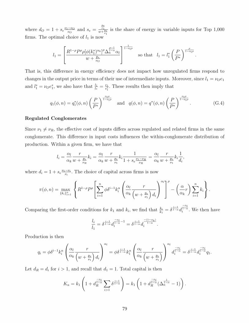
where dO = 1 + seν1−νOνO

and se =peν1

w+ peν1

is the share of energy in variable inputs for Top 1,000

firms. The optimal choice of l1 is now

l1 =

R1−ρP ρρ[φ(k∗1)αk ]ρ∆ρ−11−αn αl

w + peνO

11−αlρ

so that l1 = l∗1

(P

P ∗

) ρ1−αlρ

.

That is, this difference in energy efficiency does not impact how unregulated firms respond to

changes in the output price in terms of their use of intermediate inputs. Moreover, since l1 = νOe1

and l∗1 = νOe∗1, we also have that l1

l∗= e1

e∗1. These results then imply that

q1(φ, n) = q∗1(φ, n)

(P

P ∗

) αlρ

1−αlρ

and q(φ, n) = q∗(φ, n)

(P

P ∗

) αlρ

1−αlρ

. (G.4)

Regulated Conglomerates

Since ν1 6= νR, the effective cost of inputs differs across regulated and related firms in the same

conglomerate. This difference in input costs influences the within-conglomerate distribution of

production. Within a given firm, we have that

li =αlαk

r

w + peνR

ki =αlαk

r

w + peν1

ki1

1 + seν1−νRνR

=αlαk

r

w + peν1

ki1

di,

where di = 1 + seν1−νiνi

. The choice of capital across firms is now

π(φ, n) = maxkini=1

R1−ρP ρ

n∑i=1

φδi−1kαi

αlαk

r(w + pe

ν1

)di

αlρ − ( α

αkr

) n∑i=1

ki

.

Comparing the first-order conditions for k1 and ki, we find that kik1

= δi−11−αd

−αl1−αi . We then have

lil1

= δi−11−αd

−αl1−α−1

i = δi−11−αd

−(1−αk)1−α

i .

Production is then

qi = φδi−1kαi

αlαk

r(w + pe

ν1

)di

αl

= φδi−11−αkα1

αlαk

r(w + pe

ν1

)αl

d−αl1−αi = δ

i−11−αd

−αl1−αi q1.

Let dR = di for i > 1, and recall that d1 = 1. Total capital is then

Kn = k1

(1 + d

−αl1−αR

∑i>1

δi−11−α

)= k1

(1 + d

−αl1−αR (∆

11−αn − 1)

).

79

Define ∆n =

(1 + d

−αl1−αR (∆

11−αn − 1)

)1−α

. The analysis for the optimal choice of Kn now holds

with ∆n in place of ∆n. In the case of regulated firms, we have

q∗(φ, n) =(φ∆n

) 11−αρ

R(1−ρ)α1−αρ P ∗

ρα1−αρ ρ

α1−αρ

[(αl

w + peν1

)αl (αkr

)αk] 11−αρ

︸ ︷︷ ︸=CQ

. (G.5)

Moreover, the thresholds defining the optimal number of conglomerates in Proposition 2

continue to hold using ∆n. Note, however, that our assumption that energy costs change discon-

tinuously at φ implies that regulated and unregulated conglomerates have different thresholds

φn. Let φOn be the set of size thresholds for unregulated conglomerates and φRn be the set of

related conglomerates. Let n′ be the largest firm size for unregulated firms (so that φOn′+1 > φ)

and n′′ be the smallest size of regulated conglomerates (so that φRn′′ < φ). The combined set

of size thresholds is then φOn n′n=1, φ, φRnn=n′′+1. We include φ in this list since it is possible

that the change in energy efficiency for regulated firms leads to a change in firm size, though

(depending on the differences in energy efficiency) this may not always be the case.

Consider now the response of the firms to the regulation. Using the fact that k∗i = k∗1δi−11−αd

−αl1−αi ,

we can write the profit maximization problem as

maxlin1

R1−ρP ρ

[φ∗

n∑i=1

δ(i−1)(1−αl)

1−α lαli d−αlαk1−αi

]ρ−(w +

peν1

) n∑i=1

dili − rn∑i=1

k∗i

subject to l1 ≤ ξl∗1,

where φ∗ = φ(k∗1)αk . The first-order conditions for li (1 ≤ i ≤ n) are then

R1−ρP ρ︸ ︷︷ ︸Market Demand

ρ

[φ∗

n∑i=1

δ(i−1)(1−αl)

1−α lαli d−αlαk1−αi

]ρ−1

︸ ︷︷ ︸Residual Revenue

φ∗δ(i−1)(1−αl)

1−α αl(li)αl−1d

−αlαk1−αi︸ ︷︷ ︸

Marginal Product

=

(w +

peν1

)di + λ(φ)I[i = 1]︸ ︷︷ ︸

Shadow Cost

of Regulation

.

Taking the ratio of the conditions for l1 and li(i > 1), we have

(lil1

)1−αl= δ

(i−1)(1−αl)1−α

1 +λ(φ)(w + pe

ν1

) d−αlαk1−α −1

i

(lil1

)1−αl= δ

(i−1)(1−αl)1−α

1 +λ(φ)(w + pe

ν1

) d−(1−αl)(1−αk)

1−αi

lil1

= δ(i−1)1−α

1 +λ(φ)(w + pe

ν1

) 1

1−αl

d−(1−αk)

1−αi .

80

The residual revenue term now becomes

φ(k∗1)αk lαl1

1 +∑i>1

δi−11−αd

−αl1−αi

1 +λ(φ)(w + pe

ν1

)

αl1−αl

= φ(k∗1)αk(l∗1)αlξαl

1 + (∆1

1−αn − 1)

1 +λ(φ)(w + pe

ν1

)

αl1−αl

.The first-order condition for the regulated firm is then

R1−ρP ∗ρρ

[φ

n∑i=1

δi−11−α (k∗i )

αk(l∗i )αl

]ρ−1

× φαl(k∗1)αk(l∗1)αl−1

︸ ︷︷ ︸FOC Unregulated Case

×(ξ)αl−1

(P

P ∗

)ρξαl

1 + (∆1

1−αn − 1)

[1 + λ(φ)(

w+ peν1

)] αl

1−αl

∆1

1−αn︸ ︷︷ ︸

≡ξdq,n

ρ−1

=

(w +

peν1

)+ λ(φ),

where q(φ,n)q∗(φ,n)

= ξdq,n. Using the fact that the first-order condition in the unregulated case equals(w + pe

ν1

), we obtain

1 +λ(φ)(w + pe

ν1

) = (ξ)αl−1

(P

P ∗

)ρ(ξdq,n)(ρ−1). (G.6)

Product Market Equilibrium

The price level absent the regulation is then

P ∗−ρ = R−ρ∫ φ

φ1

((φ∆n)

11−αρ R

(1−ρ)α1−αρ P ∗

ρα1−αρCQ (dO)

−αl1−αρ

)ρ g(φ)M

1−G(φ1)dφ

+ R−ρ∫φ1

((φ∆n

) 11−αρ

R(1−ρ)α1−αρ P ∗

ρα1−αρCQ

)ρg(φ)M

1−G(φ1)dφ

P ∗−ρ

1−αρR(1−α)ρ1−αρ C−ρQ

1−G(φ1)

M=

∫ φ

φ1

(φ∆nd

−αlO

) ρ1−αρ g(φ)dφ+

∫φ

(φ∆n

) ρ1−αρ

g(φ)dφ

P ∗−ρ

1−αρR(1−α)ρ1−αρ C−ρQ

1−G(φ1)

M=

n−1∑n=1

(∆nd−αlO )

ρ1−αρπn + (∆nd

−αlO )

ρ1−αρ π1

+ (∆n)ρ

1−αρ π2 +∑n=n+1

(∆n)ρ

1−αρπn.

After the regulation, the equilibrium is then

P−ρ = R−ρ∫ φ

φ1

((P

P ∗

) αlρ

1−αlρ

(φ∆n)1

1−αρ R(1−ρ)α1−αρ P ∗

ρα1−αρCQ (dO)

−αl1−αρ

)ρ

g(φ)M

1−G(φ1)dφ

+ R−ρ∫φ

(ξdq,n

(φ∆n

) 11−αρ

R(1−ρ)α1−αρ P ∗

ρα1−αρCQ

)ρg(φ)M

1−G(φ1)dφ

81

P−ρP ∗−ρ2α1−αρR

(1−α)ρ1−αρ C−ρQ

1−G(φ1)

M=

∫ φ

φ1

(P

P ∗

) αlρ2

1−αlρ (φ∆nd

−αlO

) ρ1−αρ g(φ)dφ+

∫φ

(ξdq,n)ρ(φ∆n

) ρ1−αρ

g(φ)dφ

P−ρP ∗−ρ2α1−αρR

(1−α)ρ1−αρ C−ρQ

1−G(φ1)

M=

n−1∑n=1

(P

P ∗

) αlρ2

1−αlρ

(∆nd−αlO )

ρ1−αρπn +

(P

P ∗

) αlρ2

1−αlρ

(∆nd−αlO )

ρ1−αρ π1

+ (ξdq,n)ρ(∆n)ρ

1−αρ π2 +∑n=n+1

(ξdq,n)ρ(∆n)ρ

1−αρπn.

Comparing the regulated and unregulated equilibrium conditions, we then have

(P

P ∗

)−ρ= (1− sd

φ)

(P

P ∗

) αlρ2

1−αlρ

+ sdφEe[(ξdq,n)ρ

∣∣∣φ > φ],

where sdφ

=(∆n)

ρ1−αρ π2+

∑n=n+1

(∆n)ρ

1−αρ πn

(dO)−αlρ1−αρ

[n−1∑n=1

(∆n)ρ

1−αρ πn+(∆n)ρ

1−αρ π1

]+(∆n)

ρ1−αρ π2+

∑n=n+1

(∆n)ρ

1−αρ πn

and where Ee takes the

expectation of the distribution of energy use among regulated firms. This case differs from our

baseline case in that we use the ∆n expressions to calculate Ee.

Aggregate Energy Use

Total intermediate inputs for a regulated conglomerate are

l(φ, n)

l∗(φ, n)= ξ

[1 + (∆

11−αn − 1)d

−(1−αk)1−α

R

[1 + λ(φ)(

w+ peν1

)] 1

1−αl

]

1 + (∆1

1−αn − 1)d

−(1−αk)1−α

R

.

To compute total energy use, however, we need to take into account differences in energy efficiency

across firms in the conglomerate. Absent regulation, we have

e∗(φ, n) =l∗1ν1

+1

νR

∑i>1

l∗i =1

ν1

(l∗1 +

ν1

νR

∑i>1

l∗i

)=

1

ν1

l∗1

(1 +

ν1

νR(∆

11−αn − 1)d

−(1−αk)1−α

R

).

After the regulation, we have

e(φ, n) =1

ν1

l1

1 +ν1

νR(∆

11−αn − 1)d

−(1−αk)1−α

R

1 +λ(φ)(w + pe

ν1

) 1

1−αl

.

We then have

e(φ, n)

e∗(φ, n)= ξ

1 + ν1νR

(∆1

1−αn − 1)d

−(1−αk)1−α

R

[1 + λ(φ)(

w+ peν1

)] 1

1−αl

1 + ν1νR

(∆1

1−αn − 1)d

−(1−αk)1−α

R

≡ ξde,n.

82

To obtain an expression for e∗(φ, n) for regulated firms, recall that

l∗(φ, n) = l∗1

(1 + d

−(1−αk)1−α

R (∆1

1−αn − 1)

)

l∗(φ, n) =(φ∆n

) ρ1−αρ

R1−ρ1−αρP ∗

ρ1−αρ ρ

11−αρ

( αlw + pe

ν1

)1−αkρ (αkr

)αkρ 11−αρ

︸ ︷︷ ︸=CE

so that

e∗(φ, n) =(φ∆n

) ρ1−αρ

R1−ρ1−αρP ∗

ρ1−αρCE

1ν1

(1 + ν1

νR(∆

11−αn − 1)d

−(1−αk)1−α

R

)(

1 + d−(1−αk)

1−αR (∆

11−αn − 1)

) ,

where the last terms adjust for the composition of energy use across establishments with different

energy efficiency.

Consider now the unregulated firms. Since all firms in unregulated conglomerates have the

same energy efficiency, we have

e(φ, n)

e∗(φ, n)=

l(φ, n)

l∗(φ, n)=

(P

P ∗

) ρ1−αlρ

and

e∗(φ, n) =l∗(φ, n)

νO=

1

νO(φ∆n)

ρ1−αρ R

1−ρ1−αρP ∗

ρ1−αρ ρ

11−αρ

( αlw + pe

ν1

)1−αkρ (αkr

)αkρ 11−αρ

︸ ︷︷ ︸=CE

(dO)−(1−αkρ)

1−αρ .

The total energy use prior to the regulation is then

E∗ =

∫φ1

e∗(φ, n)g(φ)M

1−G(φ1)dφ

= R1−ρ1−αρP ∗

ρ1−αρ

CEM

1−G(φ1)

[(dO)

−(1−αkρ)1−αρ

νO

(n−1∑n=1

(∆n)ρ

1−αρ πn + (∆n)ρ

1−αρ π1

)

+(

∆n

) ρ1−αρ

1ν1

(1 + ν1

νR(∆

11−αn − 1)d

−(1−αk)1−α

R

)(

1 + d−(1−αk)

1−αR (∆

11−αn − 1)

) π2 +∑n=n+1

(∆n

) ρ1−αρ

1ν1

(1 + ν1

νR(∆

11−αn − 1)d

−(1−αk)1−α

R

)(

1 + d−(1−αk)

1−αR (∆

11−αn − 1)

) πn

.

83

The total energy use after the regulation is then

E =

∫φ1

e(φ, n)g(φ)M

1−G(φ1)dφ

= R1−ρ1−αρP ∗

ρ1−αρ

CEM

1−G(φ1)

[(P

P ∗

) ρ1−αlρ (dO)

−(1−αkρ)1−αρ

νO

(n−1∑n=1

(∆n)ρ

1−αρ πn + (∆n)ρ

1−αρ π1

)

+ ξde,n

(∆n

) ρ1−αρ

1ν1

(1 + ν1

νR(∆

11−αn − 1)d

−(1−αk)1−α

R

)(

1 + d−(1−αk)

1−αR (∆

11−αn − 1)

) π2

+∑n=n+1

ξde,n

(∆n

) ρ1−αρ

1ν1

(1 + ν1

νR(∆

11−αn − 1)d

−(1−αk)1−α

R

)(

1 + d−(1−αk)

1−αR (∆

11−αn − 1)

) πn

.The change in aggregate energy use is then

E

E∗= (1− se

φ)

(P

P ∗

) ρ1−αlρ

+ seφEe[ξde,n

∣∣∣φ > φ],

where

1− seφ

seφ

=

(dO)−(1−αkρ)

1−αρ

νO

(∑n−1n=1 (∆n)

ρ1−αρ πn + (∆n)

ρ1−αρ π1

)(

∆n

) ρ1−αρ

1ν1

(1+

ν1νR

(∆1

1−αn −1)d

−(1−αk)1−α

R

)(

1+d

−(1−αk)1−α

R (∆1

1−αn −1)

) π2 +∑

n=n+1

(∆n

) ρ1−αρ

1ν1

(1+

ν1νR

(∆1

1−αn −1)d

−(1−αk)1−α

R

)(

1+d

−(1−αk)1−α

R (∆1

1−αn −1)

) πn

and where we evaluate Ee using the conditional probabilities

Pr[n = n′

∣∣∣φ > φ]

=

(∆n′

) ρ1−αρ

1ν1

(1+

ν1νR

(∆1

1−αn′ −1)d

−(1−αk)1−α

R

)(

1+d

−(1−αk)1−α

R (∆1

1−αn′ −1)

) πn′

(∆n

) ρ1−αρ

1ν1

(1+

ν1νR

(∆1

1−αn −1)d

−(1−αk)1−α

R

)(

1+d

−(1−αk)1−α

R (∆1

1−αn −1)

) π2 +∑

n=n+1

(∆n

) ρ1−αρ

1ν1

(1+

ν1νR

(∆1

1−αn −1)d

−(1−αk)1−α

R

)(

1+d

−(1−αk)1−α

R (∆1

1−αn −1)

) πn

.

G.3 Imperfect Substitution within Conglomerates

We now consider the possibility that the outputs of affiliates within the same conglomerate are

not perfect substitutes. In particular, we assume that the conglomerate-level composite good

q(ω) can be represented as affiliate output, such that

q(ω) =

(∑i

q(ω, i)ρc

)1/ρc

, where 0 < ρ < ρc < 1.

84

The residual demand for the ith affiliate of conglomerate ω, i.e., (ω, i), is

p(ω, i) = R1−ρP ρq(ω)ρ−ρcq(ω, i)ρc−1.

The profit maximization problem for the conglomerate is now

maxlini=1,kini=1

R1−ρP ρq(φ)ρ−ρc∑i

q(φ, i)ρc − (w + pe)∑i

li − r∑i

ki

= maxlini=1,kini=1

R1−ρP ρ

[∑i

q(φ, i)ρc

]ρ/ρc− (w + pe)

∑i

li − r∑i

ki,

where q(φ, i) = φδi−1kαki lαli . The first-order conditions for l1, ...ln imply that l(φ,i)l(φ,1)

=(q(φ,i)q(φ,1)

)ρc.

Since the capital-labor ratio remains liki

= αlαk

rw+pe

, substituting into q(φ, i) allows us to express

the first-order conditions as

kik1

=lil1

=eie1

= δ(i−1)ρc1−αρc and

qiq1

= δ(i−1)1−αρc .

These expression reduce to Proposition 1 when ρc = 1. To understand how values of ρc < 1 impact

the use of inputs within the conglomerate, note that in the exponent for the first expression, a

lower value of ρc decreases the numerator and increase the denominator. Both forces work to

reduce the magnitude of the exponent such that the use of inputs depreciates more slowly in firm

rank given the same δ.

We now define ∆Cn =

[∑ni=1(δ(i−1))

ρc1−αρc

] 1−αρcρc

, so that k1Kn

= l1Ln

= 1

(∆Cn )

ρc1−αρc

. Total composite

output is then

q(φ)ρc =

(αlαk

r

w + pe

)αlρcφρc∑i

(δ(i−1)ρc)(δ(i−1)ρc1−αρc k1)αρc

=

(αlαk

r

w + pe

)αlρcφρckαρc1 (∆C

n )ρc

1−αρc =

(αlαk

r

w + pe

)αlρc(φ∆C

n )ρcKαρcn .

We can then rewrite the optimization problem as

maxKn

R1−ρP ρ

(αlαk

r

w + pe

)ραl(φ∆C

n )ρKαρn −

(αlαkr + r

)Kn,

where we represent total variable costs as (w + pe)Ln =(αlαkr)Kn. Note that this optimization

problem is exactly the same as our in baseline model, except for the new definition of ∆Cn . The

within-conglomerate revenue share is now(δi−1

∆Cn

) ρc1−αρc

, which equals the share in the case of

perfect substitution when ρc = 1. Similarly, the results of Proposition 2 continue to hold using

the new ∆Cn .

85

Regulated Conglomerates

Given φ and k∗i , we can write q(φ)ρc as

φρc∑i

(δ(i−1)ρc)(δ(i−1)ρc1−αρc k∗1)αkρclαlρci ≡ (φ(k∗1)αk)ρc

∑i

(δ(i−1)ρc)(1−αlρc)1−αρc lαlρci .

We can similarly define the short-run response as

maxlini=1

R1−ρP ρ

φ∗(∑i

δ(i−1)ρc(1−αlρc)

1−αρc lαlρci

)1/ρcρ − (w + pe)

∑i

li.

The first-order condition in this case becomes

R1−ρP ρρ

φ∗(∑i

δ(i−1)ρc(1−αlρc)

1−αρc lαlρci

)1/ρcρ−1

× φ∗δ(i−1)ρc(1−αlρc)

1−αρc αlρc(li)αlρc−1 = w + pe + λ(φ)I[i = 1].

The within-conglomerate input allocation is now

ljl2

= δ(j−2)ρc1−αρc , j > 2 and

lil1

= δ(i−1)ρc1−αρc

[1 +

λ(φ)

w + pe

] 11−αlρc

.

The conglomerate composite output is then

q(φ, n) = q1(φ, n)

[1 +

∑i>1

δ(i−1)ρc1−αρc

[1 +

λ(φ)

w + pe

] αlρc1−αlρc

]1/ρc

.

Recalling that the original preregulation optimal composite output is

q∗(φ, n) = q∗1(φ, n)

[n∑i

δ(i−1)ρc1−αρc

]1/ρc

≡ q∗1(φ, n)(∆Cn )

11−αρc

and using the fact that q1(φ, n) = q∗1(φ, n)ξαl , we obtain

q(φ, n) = q∗(φ, n)

ξαl(

1 + ((∆Cn )

ρc1−αρc − 1)

[1 + λ(φ)

w+pe

] αlρc1−αlρc

)1/ρc

(∆Cn )

11−αρc

︸ ︷︷ ︸

ξCq,n(φ)

.

Using similar arguments from our baseline model, we have that the shadow cost of the regulation

takes the form

1 +λ(φ)

w + pe= (ξ)αlρc−1

(P

P ∗

)ρ(ξCq,n)ρ−1.

86

As in previous cases, the shadow cost depends only on n. Unregulated conglomerates are not

affected by imperfect substitution within regulated conglomerates. We thus still have that

l1 = l∗1

(P

P ∗

) ρ1−αlρ

and

q(φ, n) = q∗(φ, n)

(P

P ∗

) ρ1−αlρ

.

Product Market Equilibrium

We now again define the industry price index in terms of quantity of both regulated and unreg-

ulated conglomerates. The equilibrium price is defined by

P =

[∫φ1

p(φ, n)ρρ−1

M

1−G(φ1)dG

] ρ−1ρ

where p(φ, n)ρcρc−1 =

n∑i=1

p(φ, i)ρcρc−1 .

Substituting the residual demand curve p(φ, i) = R1−ρP ρq(φ, n)ρ−ρcq(φ, i)ρc−1, we have the com-

posite conglomerate price index

p(φ, n) = R1−ρP ρq(φ, n)ρ−ρc

(∑i

q(φ, i)ρc

) ρc−1ρc

≡ R1−ρP ρq(φ, n)ρ−1.

Substituting this expression into the aggregate price index P , we have

Pρρ−1 =

∫φ1

(R1−ρP ρ)ρρ−1 q(φ, n)ρ

M

1−G(φ1)dG,

which is equivalent to P−ρ = R−ρ∫φ1q(φ, n)ρ M

1−G(φ1)dG. That is, the equation describing the

change in equilibrium prices, Equation D.7, continues to hold with the new definition of ∆Cn and

ξCq,n.

Aggregate Energy Use

Consider first the regulated conglomerate. Using the fact that e∗(φ, n) = e∗1(φ, n)∑

i δ(i−1)ρc1−αρc =

e∗1(φ, n)(∆Cn )

ρc1−αρc , we have that

e(φ, n) = e1(φ, n)

[1 +

∑i>1

δ(i−1)ρc1−αρc

[1 +

λnw + pe

] 11−αlρc

]

= e∗(φ, n)

ξ(

1 + ((∆Cn )

ρc1−αρc − 1)

[1 + λn

w+pe

] 11−αlρc

)(∆C

n )ρc

1−αρc

︸ ︷︷ ︸

ξCe,n

.

The rest of the aggregation results then similarly carry through with ξCe,n defined as above.

87

Appendix Figures

Figure A.1: Data Comparison: ASIF, CESD, Tax Data

A. Comparison of Output Data, 2001–2010

45 degree line

810

1214

16ln

(Out

put):

AS

IF &

Tax

Dat

a

8 10 12 14 16ln(Output): CESD Data

B. Comparison of Coal Consumption, 2007–2010

45 degree line

68

1012

1416

ln(C

oal C

onsu

mpt

ion)

: Tax

Dat

a

6 8 10 12 14 16ln(Coal Consumption): CESD Data

Notes: Authors’ calculations using data from ASIF, CESD and ATS. This figure shows thecomparison of output and energy consumption data between the ASIF, ATS and CESD. PanelA shows that the output data from ASIF and tax data are highly correlated with those fromCESD. This panel uses data from the ASIF in 2001–2006 and ATS in 2007–2010. Panel B showsthat coal consumption figures from the tax data almost mirror those from the CESD (tax dataare available only after 2007).

88

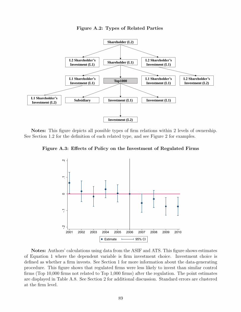
Figure A.2: Types of Related Parties

Investment (L1)

Investment (L2)

Top1000

L2 Shareholder’s

Investment (L1)

Shareholder (L2)

Subsidiary

L1 Shareholder’s

Investment (L1)

L1 Shareholder’s

Investment (L2)

Shareholder (L1)

Investment (L1)

L1 Shareholder’s

Investment (L1)

L2 Shareholder’s

Investment (L1)

L2 Shareholder’s

Investment (L2)

Notes: This figure depicts all possible types of firm relations within 2 levels of ownership.See Section 1.2 for the definition of each related type, and see Figure 2 for examples.

Figure A.3: Effects of Policy on the Investment of Regulated Firms

-.2-.1

0.1

.2

2001 2002 2003 2004 2005 2006 2007 2008 2009 2010

Estimate 95% CI

Notes: Authors’ calculations using data from the ASIF and ATS. This figure shows estimatesof Equation 1 where the dependent variable is firm investment choice. Investment choice isdefined as whether a firm invests. See Section 1 for more information about the data-generatingprocedure. This figure shows that regulated firms were less likely to invest than similar controlfirms (Top 10,000 firms not related to Top 1,000 firms) after the regulation. The point estimatesare displayed in Table A.8. See Section 2 for additional discussion. Standard errors are clusteredat the firm level.

89

Figure A.4: Innovation in Top 1,000 Firms: Energy-Saving Patent Applications

-.01

0.0

1.0

2

2001 2002 2003 2004 2005 2006 2007 2008 2009 2010

Estimate 95% CI

Notes: Authors’ calculations using data from Incopat. This figure shows estimates of Equa-tion 1 where the dependent variable is log firm patent applications. No significant effects onpatent application can be found for regulated firms relative to similar control firms (Top 10,000firms not related to Top 1,000 firms). Standard errors are clustered at the firm level.

90

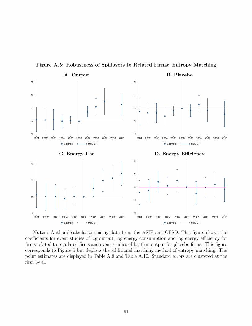
Figure A.5: Robustness of Spillovers to Related Firms: Entropy Matching

A. Output B. Placebo

-.10

.1.2

.3

2001 2002 2003 2004 2005 2006 2007 2008 2009 2010 2011

Estimate 95% CI

-.2-.1

0.1

.22001 2002 2003 2004 2005 2006 2007 2008 2009 2010 2011

Estimate 95% CI

C. Energy Use D. Energy Efficiency

-.30

.3.6

2001 2002 2003 2004 2005 2006 2007 2008 2009 2010

Estimate 95% CI

-.6-.3

0.3

.6

2001 2002 2003 2004 2005 2006 2007 2008 2009 2010

Estimate 95% CI

Notes: Authors’ calculations using data from the ASIF and CESD. This figure shows thecoefficients for event studies of log output, log energy consumption and log energy efficiency forfirms related to regulated firms and event studies of log firm output for placebo firms. This figurecorresponds to Figure 5 but deploys the additional matching method of entropy matching. Thepoint estimates are displayed in Table A.9 and Table A.10. Standard errors are clustered at thefirm level.

91

Figure A.6: Robustness to Dropping Electric Power Generation and Supply

-.10

.1.2

.3.4

2001 2002 2003 2004 2005 2006 2007 2008 2009 2010 2011

Estimate 95% CI

Notes: Authors’ calculations using data from ASIF. This figure shows the coefficients foran event study of log firm output for firms related to regulated firms where related firms arerestricted to those in industries other than electric power generation and supply. This figurecorresponds to Panel A of Figure 5 but drops all observations in the electric power generationand supply industry. The point estimates are shown in Table A.12. Standard errors are clusteredat the firm level.

92

Figure A.7: Data Quality Robustness for Related Spillovers

A. Output

-.10

.1.2

.3.4

2001 2002 2003 2004 2005 2006 2007 2008 2009 2010 2011

Estimate for Baseline 95% CI for BaselineEstimate for Leaving out 2009 95% CI for Leaving out 2009Estimate for Filling in 2009-2010 95% CI for Filling in 2009-2010

B. Placebo

-.10

.1.2

.3.4

2001 2002 2003 2004 2005 2006 2007 2008 2009 2010 2011

Estimate for Baseline 95% CI for BaselineEstimate for Leaving out 2009 95% CI for Leaving out 2009Estimate for Filling in 2009-2010 95% CI for Filling in 2009-2010

Notes: Authors’ calculations using ASIF and ATS. This figure shows the coefficients forevent studies of log firm output for related firms and placebo firms with different datasets. Thisfigure corresponds to Panels A and B in Figure 5 but drops the data for 2009 from the ASIFon the yellow line and fills in the 2009–2010 data with tax data on the green line. The pointestimates are shown in Table A.13. Standard errors are clustered at the firm level.

93

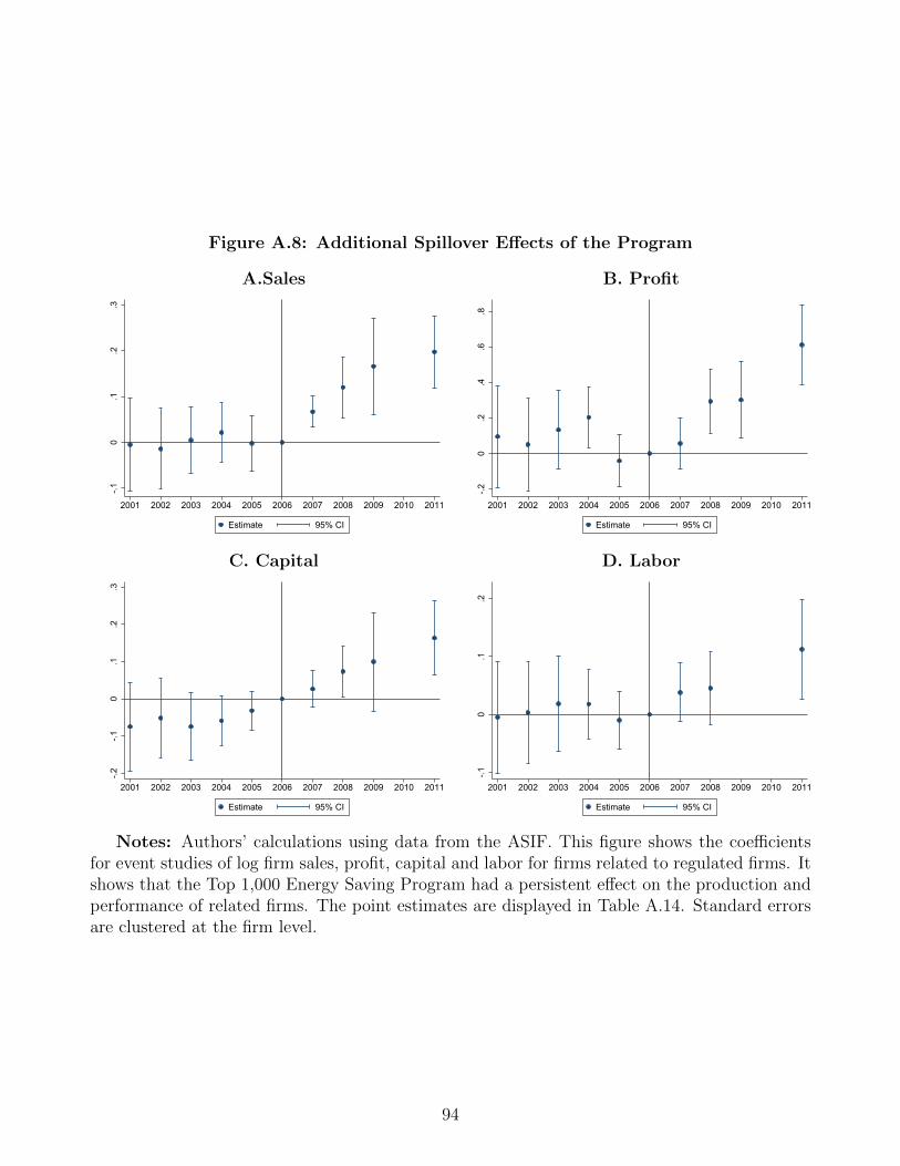
Figure A.8: Additional Spillover Effects of the Program

A.Sales B. Profit

-.10

.1.2

.3

2001 2002 2003 2004 2005 2006 2007 2008 2009 2010 2011

Estimate 95% CI

-.20

.2.4

.6.8

2001 2002 2003 2004 2005 2006 2007 2008 2009 2010 2011

Estimate 95% CI

C. Capital D. Labor

-.2-.1

0.1

.2.3

2001 2002 2003 2004 2005 2006 2007 2008 2009 2010 2011

Estimate 95% CI

-.10

.1.2

2001 2002 2003 2004 2005 2006 2007 2008 2009 2010 2011

Estimate 95% CI

Notes: Authors’ calculations using data from the ASIF. This figure shows the coefficientsfor event studies of log firm sales, profit, capital and labor for firms related to regulated firms. Itshows that the Top 1,000 Energy Saving Program had a persistent effect on the production andperformance of related firms. The point estimates are displayed in Table A.14. Standard errorsare clustered at the firm level.

94

Figure A.9: Robustness of Effects on the Energy Efficiency of Regulated Firms

-.3-.2

-.10

.1.2

.3

2001 2002 2003 2004 2005 2006 2007 2008 2009

Estimate 95% CI

Notes: Authors’ calculations using data from the CESD and ASIF. This figure shows thecoefficients for an event study of log firm energy efficiency in regulated firms, where energyefficiency is defined as the inverse of the energy share in variable input costs. Variable input iscalculated from the ASIF in terms of sales cost. This figure corresponds to Panel E of Figure 4but with an alternative definition of energy efficiency. The point estimates are shown in TableA.18. Standard errors are clustered at the firm level.

95

Figure A.10: Robustness of Effects on the Energy Efficiency of Related Firms

-.6-.4

-.20

.2.4

.6

2001 2002 2003 2004 2005 2006 2007 2008 2009

Estimate 95% CI

Notes: Authors’ calculations using data from the CESD and ASIF. This figure shows thecoefficients for an event study of log firm energy efficiency in firms related to regulated firms,where energy efficiency is defined as the inverse of the energy share in variable input costs.Variable input is calculated from the ASIF in terms of sales cost. This figure corresponds toPanel D of Figure 5 but with an alternative definition of energy efficiency. The point estimatesare shown in Table A.19. Standard errors are clustered at the firm level.

96

Appendix Tables

Table A.1: Policy Compliance

Type Orig.list Evaluation

Year 2007 2008 2009 2010Firm number 1008 953 922 901 881Noncompliant firms - 74 36 28 15Noncompliance rate - 7.76% 3.90% 3.11% 1.70%

Notes: Authors’ calculations using data from the NDRC. This table shows the compliance ofTop 1,000 firms during the 11FYP. The first row shows the number of Top 1,000 firms evaluatedby the government in each year, the second row shows the number of noncompliant firms, andthe last row shows the corresponding noncompliance rate. By the end of the 11FYP, 98.3% ofevaluated Top 1,000 firms achieved their energy saving targets. See Section 1.1 for additionaldiscussion.

Table A.2: Dataset Matching

DatasetsTop 1,000 Top 10,000

Number Ratio Number Ratio

List 1008 - 14641 -ASIF 1001 99.31% 14300 97.67%CESD 818 81.15% 10722 73.23%ASIF & CESD 809 80.26% 9481 64.76%ASIF & ATS 446 44.25% 6622 45.23%

Notes: Authors’ calculations using data from the ASIF, CESD and ATS. This table shows theresult of dataset matching. Over 99% of the Top 1,000 firms and over 97% of the Top 10,000firms can be found in the ASIF, and over 80% of the Top 1,000 firms and over 70% of the Top10,000 firms can be found in the CESD. See Section 1.2 for additional discussion.

97

Table A.3: Robustness to Dropping Electricity-Intensive Industries

Variables ln(Energy Use) ln(Output) ln(Energy Efficiency)

Electricity<15% -0.123** -0.207*** -0.083*(0.049) (0.046) (0.048)

Electricity<20% -0.133*** -0.178*** -0.045(0.050) (0.045) (0.050)

Electricity<25% -0.146*** -0.195*** -0.048(0.048) (0.043) (0.047)

Electricity<30% -0.156*** -0.204*** -0.049(0.047) (0.042) (0.046)

Electricity<35% -0.166*** -0.202*** -0.037(0.045) (0.041) (0.045)

Electricity<40% -0.164*** -0.199*** -0.036(0.045) (0.041) (0.045)

Electricity<45% -0.165*** -0.200*** -0.037(0.045) (0.041) (0.045)

Electricity<50% -0.170*** -0.233*** -0.064(0.043) (0.042) (0.045)

Firm FE Y Y YIndustry × Year FE Y Y YProvince × Year FE Y Y Y

Notes: Authors’ calculations using data from the CESD. This table reports the estimates fromregressions of log firm energy consumption, output and energy efficiency on regulated firmsinteracted with an indicator for years after 2006 under varying data restrictions. The estimatesshown in this table correspond to Equation 2 and the baseline estimates in Table 3 with theexclusion of various industries with electricity consumption accounting for more than 15%, 20%,25%, 35%, 40%, 45%, or 50% (our baseline setting is 30%). Standard errors clustered at the firmlevel are shown in parentheses with p-values below. * p<0.1, ** p<0.05, *** p<0.01.

98

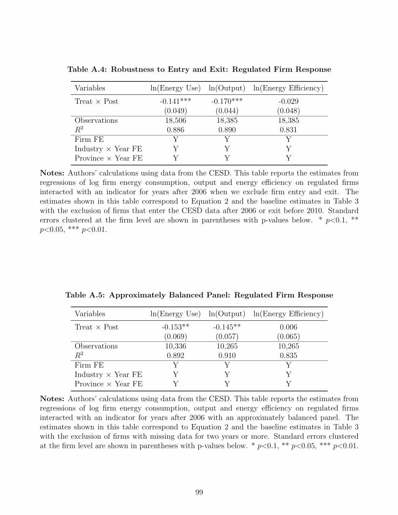
Table A.4: Robustness to Entry and Exit: Regulated Firm Response

Variables ln(Energy Use) ln(Output) ln(Energy Efficiency)

Treat × Post -0.141*** -0.170*** -0.029(0.049) (0.044) (0.048)

Observations 18,506 18,385 18,385R2 0.886 0.890 0.831Firm FE Y Y YIndustry × Year FE Y Y YProvince × Year FE Y Y Y

Notes: Authors’ calculations using data from the CESD. This table reports the estimates fromregressions of log firm energy consumption, output and energy efficiency on regulated firmsinteracted with an indicator for years after 2006 when we exclude firm entry and exit. Theestimates shown in this table correspond to Equation 2 and the baseline estimates in Table 3with the exclusion of firms that enter the CESD data after 2006 or exit before 2010. Standarderrors clustered at the firm level are shown in parentheses with p-values below. * p<0.1, **p<0.05, *** p<0.01.

Table A.5: Approximately Balanced Panel: Regulated Firm Response

Variables ln(Energy Use) ln(Output) ln(Energy Efficiency)

Treat × Post -0.153** -0.145** 0.006(0.069) (0.057) (0.065)

Observations 10,336 10,265 10,265R2 0.892 0.910 0.835Firm FE Y Y YIndustry × Year FE Y Y YProvince × Year FE Y Y Y

Notes: Authors’ calculations using data from the CESD. This table reports the estimates fromregressions of log firm energy consumption, output and energy efficiency on regulated firmsinteracted with an indicator for years after 2006 with an approximately balanced panel. Theestimates shown in this table correspond to Equation 2 and the baseline estimates in Table 3with the exclusion of firms with missing data for two years or more. Standard errors clusteredat the firm level are shown in parentheses with p-values below. * p<0.1, ** p<0.05, *** p<0.01.

99

Table A.6: Robustness to Consideration of Concurrent Policies

A. Effects of Concurrent Policies on Top 1,000 Firms

ln(Energy Use) ln(Output) ln(Energy Efficiency)

Monitor × Post -0.003 0.023 0.019(0.097) (0.089) (0.106)

Observations 3,358 3,322 3,322R2 0.865 0.899 0.812Firm FE Y Y YIndustry × Year FE Y Y YProvince × Year FE Y Y Y

B. Robustness to Effects on Top 1,000 Firms

ln(Energy Use) ln(Output) ln(Energy Efficiency)

Treat × Post -0.186** -0.234*** -0.046(0.075) (0.080) (0.083)

Observations 20,655 20,511 20,511R2 0.864 0.858 0.847Firm FE Y Y YIndustry × Year FE Y Y YProvince × Year FE Y Y Y

Notes: Authors’ calculations using data from the CESD. This table shows that our estimatedeffects of the Top 1000 program are robust to consideration of a concurrent policy—the NationalSpecially Monitored Firms (NSMF) program. Panel A estimates a difference-in-differences modelto show the effects of the NSMF program within the Top 1,000 firm sample. We can see thatthe NSMF program had little effect on the energy consumption, output and energy efficiency ofTop 1,000 firms. Panel B estimates the same regression as in Table 3 while excluding all treatedfirms included under both polices. It shows that taking the NSMF program into account doesnot affect our main results. See Section B for both detailed description of the NSMF programand additional discussion. Standard errors clustered at the firm level are shown in parentheseswith p-values below. * p<0.1, ** p<0.05, *** p<0.01.

100

Table A.7: Heterogeneous Effects on Regulated Firms by Industry

Variablesln(Output)

Baseline Drop Power Processing Materials Mining

Treat × Post -0.204*** -0.206*** -0.219*** -0.153*** -0.251(0.042) (0.042) (0.073) (0.053) (0.275)

Observations 22,991 21,748 5,440 12,662 545R2 0.889 0.887 0.893 0.865 0.863Firm FE Y Y Y Y YIndustry × Year FE Y Y Y Y YProvince × Year FE Y Y Y Y Y

Notes: Authors’ calculations using data from the CESD. This table shows estimates of Equation2 by industry where Treat × Post is an indicator for regulated firms interacted with an indicatorfor years after 2006 and the dependent variable is log firm output, corresponding to Panel Bof Table 3. Column (1) is our baseline result. Column (2) shows the results after we drop theproduction and supply of electric power and heating power industry. Column (3) shows theresults for processing industries, including smelting and pressing of ferrous metals, smelting andpressing of nonferrous metals, processing of petroleum, coking, and processing of nuclear fuel.Column (4) shows the result for material industries, including the manufacture of raw chemicalmaterials and chemical products and the manufacture of nonmetallic mineral products. Column(5) shows the result for mining industries, including mining and washing of coal and extraction ofpetroleum and natural gas. This table shows no significant differences in regulated firm responseamong different industries. Standard errors clustered at the firm level are shown in parentheseswith p-values below. * p<0.1, ** p<0.05, *** p<0.01.

101

Table A.8: Effects of Policy on Investment in Regulated Firms

Variables If Firm Invest

Treat × Post -0.056*** -0.070*** -0.070*** -0.071***(0.013) (0.014) (0.014) (0.014)

Observations 47,231 47,211 47,208 45,675R2 0.192 0.201 0.209 0.214Firm FE Y Y Y YYear FE Y Y Y YIndustry × Year FE Y Y YProvince × Year FE Y YFirm-level Controls Y

Notes: Authors’ calculations using ASIF and ATS. This table shows estimates of Equation 2where Treat × Post is an indicator for regulated firms interacted with an indicator for yearsafter 2006 and the dependent variable is firm investment choice. Investment choice is defined aswhether a firm invests. See Section 1 for more information about the data-generating procedure.This table corresponds to a pooled version of the regression displayed in Figure A.3. It showsthat regulated firms decrease their possibility of investment by 5.6%–7.1% relative to similarcontrol firms (Top 10,000 firms not related to Top 1,000 firms) after the policy implementation.See Section 2 for additional discussion. Standard errors clustered at the firm level are shown inparentheses with p-values below. * p<0.1, ** p<0.05, *** p<0.01.

102

Table A.9: Robustness of Spillovers to Related Firms on Output: Entropy Matching

A. Output

Variables ln(Output)

Related × Post 0.143*** 0.139*** 0.106*** 0.133***(0.039) (0.038) (0.037) (0.036)

Observations 119,064 119,064 119,064 116,064R2 0.874 0.881 0.890 0.896

B. Placebo Test on Output

Variables ln(Output)

Related × Post 0.016 0.019 0.020 0.036(0.041) (0.040) (0.039) (0.038)

Observations 150,997 150,997 150,997 147,431R2 0.909 0.914 0.922 0.929

C. Heterogeneous Effects on Output by Firm Size

Variables ln(Output)

Related × Post(0%-30%) 0.097 0.096 0.001 0.039(0.070) (0.068) (0.065) (0.063)

Related × Post(30%-60%) 0.171*** 0.166*** 0.123** 0.156***(0.060) (0.058) (0.054) (0.053)

Related × Post(60%-100%) 0.178*** 0.172*** 0.179*** 0.191***(0.058) (0.056) (0.054) (0.052)

Observations 95,258 95,258 95,258 92,847R2 0.874 0.881 0.891 0.897Firm FE Y Y Y YYear FE Y Y Y YIndustry × Year FE Y Y YProvince × Year FE Y YFirm-level Controls Y

Notes: Authors’ calculations using data from the ASIF. This table shows estimates of Equation2 with an alternative matching method, where Related × Post is an indicator for related firms inthe same 4-digit industry interacted with an indicator for years after 2006 in Panels A and C andan indicator for related firms in the same 2-digit industry (but not the same 4-digit industry)interacted with an indicator for years after 2006 in Panel B. This table corresponds to Table 4but deploys the additional matching method of entropy matching. Panels A and B correspondto a pooled version of the regression displayed in Panels A and B of Figure A.5. Standard errorsclustered at the firm level are shown in parentheses with p-values below. * p<0.1, ** p<0.05,*** p<0.01.

103

Table A.10: Robustness of Spillovers to Related Firms on Energy Use and EnergyEfficiency: Entropy Matching

A. Energy Use

Variables ln(Energy Use)

Related × Post 0.247** 0.248*** 0.289*** 0.263**(0.097) (0.095) (0.090) (0.104)

Observations 20,254 20,254 20,101 14,507R2 0.855 0.858 0.871 0.879

B. Energy Efficiency

Variables ln(Energy Efficiency)

Related × Post -0.021 -0.019 -0.056 -0.039(0.099) (0.098) (0.103) (0.104)

Observations 20,122 20,122 19,971 14,424R2 0.822 0.826 0.839 0.845Firm FE Y Y Y YYear FE Y Y Y YIndustry × Year FE Y Y YProvince × Year FE Y YFirm-level Controls Y

Notes: Authors’ calculations using data from the CESD and ASIF. This table shows estimatesof Equation 2 with an alternative matching method, where Related × Post is an indicator forrelated firms in the same 4-digit industry interacted with an indicator for years after 2006 and thedependent variables are log firm energy consumption in Panel A and log firm energy efficiencyin Panel B. This table corresponds to Table 5 but deploys the additional matching method ofentropy matching and corresponds to a pooled version of the regression displayed in Panels Cand D of Figure A.5. Standard errors clustered at the firm level are shown in parentheses withp-values below. * p<0.1, ** p<0.05, *** p<0.01.

104

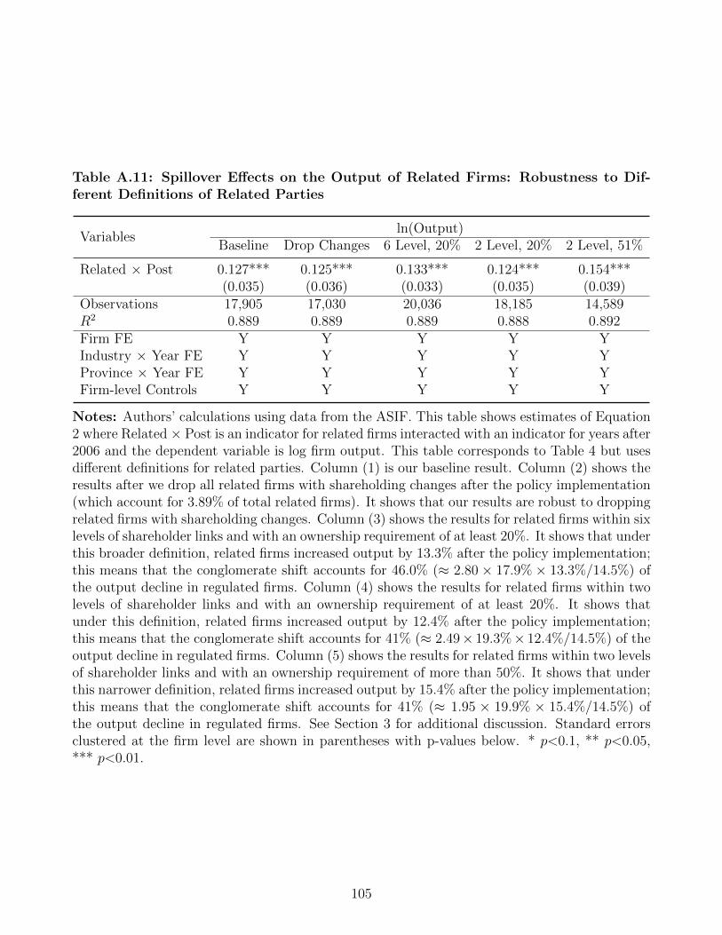
Table A.11: Spillover Effects on the Output of Related Firms: Robustness to Dif-ferent Definitions of Related Parties

Variablesln(Output)

Baseline Drop Changes 6 Level, 20% 2 Level, 20% 2 Level, 51%

Related × Post 0.127*** 0.125*** 0.133*** 0.124*** 0.154***(0.035) (0.036) (0.033) (0.035) (0.039)

Observations 17,905 17,030 20,036 18,185 14,589R2 0.889 0.889 0.889 0.888 0.892Firm FE Y Y Y Y YIndustry × Year FE Y Y Y Y YProvince × Year FE Y Y Y Y YFirm-level Controls Y Y Y Y Y

Notes: Authors’ calculations using data from the ASIF. This table shows estimates of Equation2 where Related× Post is an indicator for related firms interacted with an indicator for years after2006 and the dependent variable is log firm output. This table corresponds to Table 4 but usesdifferent definitions for related parties. Column (1) is our baseline result. Column (2) shows theresults after we drop all related firms with shareholding changes after the policy implementation(which account for 3.89% of total related firms). It shows that our results are robust to droppingrelated firms with shareholding changes. Column (3) shows the results for related firms within sixlevels of shareholder links and with an ownership requirement of at least 20%. It shows that underthis broader definition, related firms increased output by 13.3% after the policy implementation;this means that the conglomerate shift accounts for 46.0% (≈ 2.80 × 17.9% × 13.3%/14.5%) ofthe output decline in regulated firms. Column (4) shows the results for related firms within twolevels of shareholder links and with an ownership requirement of at least 20%. It shows thatunder this definition, related firms increased output by 12.4% after the policy implementation;this means that the conglomerate shift accounts for 41% (≈ 2.49× 19.3%× 12.4%/14.5%) of theoutput decline in regulated firms. Column (5) shows the results for related firms within two levelsof shareholder links and with an ownership requirement of more than 50%. It shows that underthis narrower definition, related firms increased output by 15.4% after the policy implementation;this means that the conglomerate shift accounts for 41% (≈ 1.95 × 19.9% × 15.4%/14.5%) ofthe output decline in regulated firms. See Section 3 for additional discussion. Standard errorsclustered at the firm level are shown in parentheses with p-values below. * p<0.1, ** p<0.05,*** p<0.01.

105

Table A.12: Robustness to Dropping Electric Power Generation and Supply

Variables ln(Output)

Related*Post 0.180*** 0.173*** 0.163*** 0.167***(0.043) (0.041) (0.039) (0.037)

Observations 11,232 11,229 11,222 10,982R2 0.850 0.862 0.872 0.883Firm FE Y Y Y YYear FE Y Y Y YIndustry × Year FE Y Y YProvince × Year FE Y YFirm-level Controls Y

Notes: Authors’ calculations using data from the ASIF. This table shows estimates of Equation2 where Related × Post is an indicator for related firms in industries other than electric powergeneration and supply interacted with an indicator for years after 2006 and the dependent variableis log firm output. This table corresponds to Panel A of Table 4 but with the exclusion of allfirms in the electric power generation and supply industry and corresponds to a pooled versionof the regression displayed in Figure A.6. Standard errors clustered at the firm level are shownin parentheses with p-values below. * p<0.1, ** p<0.05, *** p<0.01.

106

Table A.13: Data Quality Robustness of Spillovers to Related Firms

A. Output: Leave out 2009 in ASIF Data

Variables ln(Output)

Related × Post 0.131*** 0.125*** 0.102*** 0.111***(0.034) (0.033) (0.033) (0.031)

Observations 16,454 16,452 16,450 15,970R2 0.890 0.898 0.905 0.913

B. Output: Fill in 2009–2010 with Tax Data

Variables ln(Output)

Related × Post 0.159*** 0.156*** 0.137*** 0.135***(0.037) (0.037) (0.037) (0.035)

Observations 19,293 19,289 19,287 18,735R2 0.869 0.876 0.885 0.893

C. Placebo: Leave out 2009 in ASIF Data

Variables ln(Output)

Related × Post -0.033 -0.031 -0.025 -0.019(0.039) (0.037) (0.038) (0.037)

Observations 7,971 7,970 7,955 7,809R2 0.908 0.914 0.921 0.927

D. Placebo: Fill in 2009–2010 with Tax Data

Variables ln(Output)

Related × Post 0.000 -0.003 -0.005 -0.007(0.041) (0.040) (0.040) (0.039)

Observations 9,289 9,288 9,268 9,104R2 0.875 0.880 0.889 0.897Firm FE Y Y Y YYear FE Y Y Y YIndustry × Year FE Y Y YProvince × Year FE Y YFirm-level Controls Y

Notes: Authors’ calculations using ASIF and tax data. This table shows estimates of Equation2 with different datasets, where Related × Post is an indicator for related firms in the same4-digit industry interacted with an indicator for years after 2006, and the dependent variable islog firm output. Panels A and C correspond to Panels A and B in Table 4 but with the exclusionof the 2009 data from the ASIF. Panels B and D correspond to Panels A and B in Table 4 butwith the 2009–2010 data filled in with tax data. The estimates in this table also correspond toa pooled version of the regression displayed in Figure A.7. Standard errors clustered at the firmlevel are shown in parentheses with p-values below. * p<0.1, ** p<0.05, *** p<0.01.

107

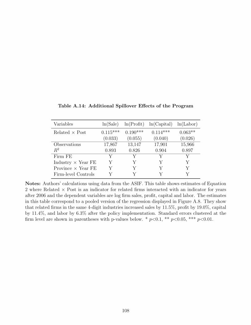
Table A.14: Additional Spillover Effects of the Program

Variables ln(Sale) ln(Profit) ln(Capital) ln(Labor)

Related × Post 0.115*** 0.190*** 0.114*** 0.063**(0.033) (0.055) (0.040) (0.026)

Observations 17,867 13,147 17,901 15,966R2 0.893 0.826 0.904 0.897Firm FE Y Y Y YIndustry × Year FE Y Y Y YProvince × Year FE Y Y Y YFirm-level Controls Y Y Y Y

Notes: Authors’ calculations using data from the ASIF. This table shows estimates of Equation2 where Related × Post is an indicator for related firms interacted with an indicator for yearsafter 2006 and the dependent variables are log firm sales, profit, capital and labor. The estimatesin this table correspond to a pooled version of the regression displayed in Figure A.8. They showthat related firms in the same 4-digit industries increased sales by 11.5%, profit by 19.0%, capitalby 11.4%, and labor by 6.3% after the policy implementation. Standard errors clustered at thefirm level are shown in parentheses with p-values below. * p<0.1, ** p<0.05, *** p<0.01.

108

Table A.15: Spillover Effects on the Output of Related Firms: Heterogeneous Effectsby Industry

Variablesln(Output)

Baseline Drop Power Processing Materials Mining

Related × Post 0.118*** 0.164*** 0.105 0.180*** 0.197**(0.037) (0.040) (0.096) (0.056) (0.080)

Observations 18,418 11,152 2,586 5,566 2,641R2 0.881 0.872 0.871 0.846 0.883Firm FE Y Y Y Y YIndustry × Year FE Y Y Y Y YProvince × Year FE Y Y Y Y Y

Notes: Authors’ calculations using data from the ASIF. This table shows estimates of Equation2 by industry where Related × Post is an indicator for related firms interacted with an indicatorfor years after 2006 and the dependent variable is log firm output, corresponding to Panel Aof Table 4. Column (1) is our baseline result. Column (2) shows the results after we drop theproduction and supply of electric power and heat power industry. Column (3) shows the resultfor processing industries, including smelting and pressing of ferrous metals, smelting and pressingof nonferrous metals, processing of petroleum, coking, and processing of nuclear fuel. Column(4) shows the result for material industries, including manufacture of raw chemical materialsand chemical products and manufacture of nonmetallic mineral products. Column (5) shows theresults for mining industries, including mining and washing of coal and extraction of petroleumand natural gas. This table shows that we do not find significant differences in the response ofrelated firms across different industries. Standard errors clustered at the firm level are shown inparentheses with p-values below. * p<0.1, ** p<0.05, *** p<0.01.

109

Table A.16: Robustness to Entry: Market Spillovers

Variablesln(Output)

All Sample Energy-intensive Industries

Spillover × Post 0.083*** 0.075*** 0.092*** 0.092***(0.022) (0.020) (0.021) (0.025)

Observations 2,129,911 2,129,911 716,518 716,518R2 0.847 0.862 0.837 0.853Firm FE Y Y Y YYear FE Y Y Y YIndustry-level Controls Y Y Y YFirm-level Controls Y Y

Notes: Authors’ calculations using data from the ASIF. This table shows estimates of Equation3 where Spillover × Post is an indicator for industry-level exposure to the Top 1,000 programinteracted with an indicator for years after 2006 and the dependent variable is log firm output.This table corresponds Table 6 with the exclusion of firms that enter the CESD data after 2006. Itshows that average market-level spillovers led to a 7.5%–9.2% increase in output for unregulatedexisting firms. See Section 3 for additional discussion. Standard errors clustered at the firm levelare shown in parentheses with p-values below. * p<0.1, ** p<0.05, *** p<0.01.

110

Table A.17: Structural Estimation: Robustness to Alternative Specifications

Data Baseline Low ρ High ρ Low α High α ImperfectSubstitution

1. Fixed ValuesElasticity of substitution ρ 0.750 0.700 0.900 0.750 0.750 0.750Within-conglomerate 0.900Elasticity of substitution ρcReturn to scale α 0.900 0.900 0.900 0.850 0.950 0.9002. Method of MomentsEfficiency depreciation δ 0.900 0.900 0.900 0.853 0.949 0.800

(0.003) (0.003) (0.003) (0.005) (0.001) (0.007)Dispersion of ln-ability σm 1.239 1.500 0.579 1.359 1.063 1.271

(0.055) (0.060) (0.045) (0.087) (0.053) (0.097)Survival threshold φ1 0.609 0.461 0.792 0.579 0.435 0.985

(0.166) (0.134) (0.193) (0.273) (0.118) (0.535)3. Policy Parameters

Policy threshold φ 9.289 14.093 2.658 10.915 6.050 10.9774. MomentsShare of firms < 1M 0.336 0.347 0.350 0.350 0.347 0.351 0.344Share of firms 5− 20M 0.105 0.155 0.155 0.160 0.157 0.156 0.156Share of firms 20− 100M 0.071 0.072 0.072 0.076 0.073 0.074 0.071Share of firms 100M+ 0.025 0.026 0.026 0.027 0.027 0.027 0.025Share of Output 5− 20M 0.051 0.072 0.072 0.074 0.073 0.073 0.072Share of Output 20− 100M 0.146 0.144 0.144 0.152 0.147 0.148 0.142Share of Output 100M+ 0.722 0.733 0.733 0.723 0.729 0.729 0.734Relative Output 1st-2nd 0.289 0.348 0.350 0.347 0.347 0.350 0.347Relative Output 2nd-3rd 0.203 0.121 0.122 0.120 0.120 0.122 0.121

Notes: This table summarizes the parameters that we set or estimate. Panel 1 lists the variousparameter values that we calibrate. Across all cases, we set αl to match the cost share ofvariable inputs, given α. Panel 2 reports the estimated parameter moments with standard errorsin parentheses. See Section 5.1 for the detailed estimation procedure. Panel 3 reports thepolicy threshold φ. This threshold is selected to match the share of energy use by regulatedfirms, which itself depends on the parameter values. Panel 4 reports the data moments and themoments predicted by the model parameters. Section 7.3 discusses the results when we vary αor ρ, and Section 7.4 discusses the results when we set ρc = 0.9.

111

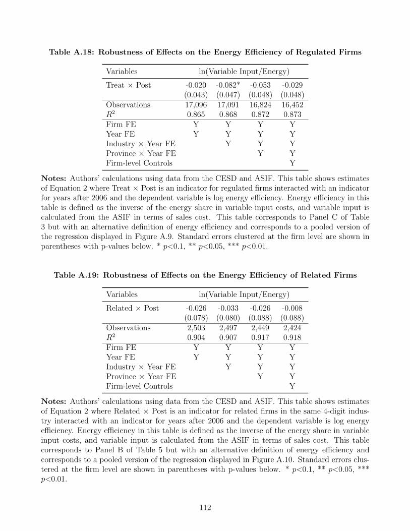
Table A.18: Robustness of Effects on the Energy Efficiency of Regulated Firms

Variables ln(Variable Input/Energy)

Treat × Post -0.020 -0.082* -0.053 -0.029(0.043) (0.047) (0.048) (0.048)

Observations 17,096 17,091 16,824 16,452R2 0.865 0.868 0.872 0.873Firm FE Y Y Y YYear FE Y Y Y YIndustry × Year FE Y Y YProvince × Year FE Y YFirm-level Controls Y

Notes: Authors’ calculations using data from the CESD and ASIF. This table shows estimatesof Equation 2 where Treat × Post is an indicator for regulated firms interacted with an indicatorfor years after 2006 and the dependent variable is log energy efficiency. Energy efficiency in thistable is defined as the inverse of the energy share in variable input costs, and variable input iscalculated from the ASIF in terms of sales cost. This table corresponds to Panel C of Table3 but with an alternative definition of energy efficiency and corresponds to a pooled version ofthe regression displayed in Figure A.9. Standard errors clustered at the firm level are shown inparentheses with p-values below. * p<0.1, ** p<0.05, *** p<0.01.

Table A.19: Robustness of Effects on the Energy Efficiency of Related Firms

Variables ln(Variable Input/Energy)

Related × Post -0.026 -0.033 -0.026 -0.008(0.078) (0.080) (0.088) (0.088)

Observations 2,503 2,497 2,449 2,424R2 0.904 0.907 0.917 0.918Firm FE Y Y Y YYear FE Y Y Y YIndustry × Year FE Y Y YProvince × Year FE Y YFirm-level Controls Y

Notes: Authors’ calculations using data from the CESD and ASIF. This table shows estimatesof Equation 2 where Related × Post is an indicator for related firms in the same 4-digit indus-try interacted with an indicator for years after 2006 and the dependent variable is log energyefficiency. Energy efficiency in this table is defined as the inverse of the energy share in variableinput costs, and variable input is calculated from the ASIF in terms of sales cost. This tablecorresponds to Panel B of Table 5 but with an alternative definition of energy efficiency andcorresponds to a pooled version of the regression displayed in Figure A.10. Standard errors clus-tered at the firm level are shown in parentheses with p-values below. * p<0.1, ** p<0.05, ***p<0.01.

112

Table A.20: Heterogeneous Spillover Effects by Local Pollution and Density

Variable High to Low Horizontal Low to High

Related × Post 0.115** 0.101 0.224***(0.047) (0.072) (0.073)

Observations 10,256 3,740 3,457R2 0.895 0.883 0.897Output Share 57.9% 13.9% 28.2%Aggregate Effect 6.7% 1.4% 6.3%Firm FE Y Y YYear FE Y Y YIndustry × Year FE Y Y YProvince × Year FE Y Y YFirm-level Controls Y Y Y

Notes: Authors’ calculations using data from the ASIF. This table show estimates of Equation 2where Related × Post is an indicator for related firms in the same 4-digit industry interacted withan indicator for years after 2006 and the dependent variable is log firm output. The estimatescorrespond to Panel A of Table 4 but divide related firms into three groups according to theirpollution exposure. Column (1) includes related firms whose city-level pollution exposure is lessthan (by more than 10%) that of their corresponding Top 1,000 firms; Column (2) includes relatedfirms whose city-level pollution exposure is similar to (within 10%) that of their correspondingTop 1,000 firms; and Column (3) includes related firms whose city-level pollution exposure ismore than (by more than 10%) that of their corresponding Top 1,000 firms. City-level pollutionexposure is defined by city-level so2 density× city population. This table shows that related firmsin places with lower pollution exposure increased output by 11.5% and related firms in placeswith similar pollution exposure increased output by 10.1% while related firms in places withmore pollution exposure increased output by 22.4% after the policy implementation. However,considering that a higher share of the related output (57.9%) was concentrated in less exposedareas, we see similar output increases in more and less exposed areas. See Section C for additionaldiscussion. Standard errors clustered at the firm level are shown in parentheses with p-valuesbelow. * p<0.1, ** p<0.05, *** p<0.01.

113