NBER WORKING PAPER SERIES

RESOURCE ALLOCATION WITHIN FIRMS AND FINANCIAL MARKET DISLOCATION:EVIDENCE FROM DIVERSIFIED CONGLOMERATES

Gregor MatvosAmit Seru

Working Paper 17717http://www.nber.org/papers/w17717

NATIONAL BUREAU OF ECONOMIC RESEARCH1050 Massachusetts Avenue

Cambridge, MA 02138December 2011

We are grateful to the Initiative on Global Markets and the Fama-Miller Center at the University ofChicago Booth School of Business for funding. The views expressed herein are those of the authorsand do not necessarily reflect the views of the National Bureau of Economic Research.

NBER working papers are circulated for discussion and comment purposes. They have not been peer-reviewed or been subject to the review by the NBER Board of Directors that accompanies officialNBER publications.

© 2011 by Gregor Matvos and Amit Seru. All rights reserved. Short sections of text, not to exceedtwo paragraphs, may be quoted without explicit permission provided that full credit, including © notice,is given to the source.

Resource Allocation within Firms and Financial Market Dislocation: Evidence from DiversifiedConglomeratesGregor Matvos and Amit SeruNBER Working Paper No. 17717December 2011JEL No. D92,E22,G01,G3,L21,L25

ABSTRACT

When external capital markets are stressed they may not reallocate resources between firms. We showthat resource allocation within firms' internal capital markets provides an important force countervailingfinancial market dislocation. Using data on US conglomerates we empirically verify that firms shiftresources between industries in response to shocks to the financial sector. We estimate a structuralmodel of internal capital market to separately identify and quantify the forces driving the reallocationdecision and how these forces interact with external capital market stress. The frictions in internalcapital markets drive a large wedge between productivity and investment: the weaker (stronger) divisionobtains too much (little) capital, as though it is 12 (9) percent more (less) productive than it reallyis. The cost of accessing external capital funds quadruple during extreme financial market dislocations,making resource allocation within firms significantly cheaper. The estimated model allows us to simulatethe propagation of the 2007/2008 financial market dislocation. The counterfactual out of sample simulateddata is remarkably consistent with the actual data and shows that improved resource allocation in internalcapital markets offset financial market stress during the recent financial crisis by 16% to 30% relativeto firms with no internal capital markets.

Gregor MatvosBooth School of BusinessUniversity of Chicago5807 South Woodlawn AvenueChicago, IL 60637and NBERgmatvos@chicagobooth.edu

Amit SeruBooth School of BusinessUniversity of Chicago5807 South Woodlawn AvenueChicago, IL 60637and NBERamit.seru@chicagobooth.edu

I Introduction

Do firm boundaries mediate the effect of shocks to the financial intermediation sector? When the

functioning of the intermediation sector is impaired —as was the case in the recent financial crisis

—shocks can be transmitted to the broader economy since funds may not flow to highest value use

without incurring significant cost. This issue has been extensively explored in the credit channel

literature (e.g., Kashyap and Stein [2000]; Bernanke and Blinder [1988; 1992] and Bernanke and

Gertler [1995]). However, unlike what is assumed in this literature, firms may be able to reallocate

resources internally — for instance, between divisions in different industries — to ameliorate the

effect of financial shocks. If so, external credit market conditions will impact the nature of resource

allocation inside firms and between industries differently than they would in an economy with no

internal capital markets. Diversified firms constitute a large part of economies around the world,1

therefore resource allocation within firms can be of significant importance in determining macro

outcomes such as business cycle fluctuations, total factor productivity and growth (eg. Bloom

[2009]). In this paper we propose and empirically verify that firms shift resources between industries

in response to shocks to the financial sector. We then estimate a structural model to quantify the

forces driving this reallocation decision, and show that these forces dampen shocks to the financial

sector in economically significant ways.2

We study the resource allocation problem in a sample of diversified firms in the U.S. Economists

have used these firms as a laboratory for studying resource allocation decisions inside firms. There

are two prevailing views on how capital is internally allocated in these firms. Alchian [1969] and

Stein [1997], among others, have put forth the view that conglomerates may outperform external

capital markets by virtue of exerting centralized control over the capital allocation process (‘bright

side’view). This view has been challenged by several studies, such as Rajan, Servaes and Zingales

[2000] and Scharfstein and Stein [2000] who argue that resource allocation inside firms is distorted

towards weaker divisions by managerial socialistic concerns (‘dark side’view). We propose and es-

timate a model with a dynamic tradeoff between the ‘bright’and the ‘dark’side of internal capital

markets. In our setting, the cost of conglomerates arises from managerial preferences for corporate

socialism. The benefit is that funds can be allocated between divisions without experiencing fric-

tions of accessing external capital markets. The cost of accessing external capital markets vary over

time introducing a time varying wedge between the cost and benefit of internal capital markets.

We first present reduced form evidence that motivate the economic forces in our structural

model using data of diversified firms in the US from 1980 to 2006. We show that conglomerates’

performance relative to stand-alone firms improves during times in which external capital markets

are impaired. Moreover, during these periods, conglomerates with more productivity dispersion

among their divisions perform relatively better. Figure 1 plots the value of conglomerates with high

1The Bureau of the Census reports that multi-industry firms account for about half of the sales in the U.S in 2008.2To our knowledge, this is the first paper to estimate a structural model of capital allocation within conglomerates.

For other structural models with credit market frictions see Einav, Jenkins and Levin [2010], Whited [2006], and Bloom[2009].

1

productivity dispersion relative to the value of conglomerates with low productivity dispersion. It

shows that the difference in these values narrows with an increase in the TED spread, our measure

of external capital market distress. We also show that these valuation results are correlated with

changes in capital allocation across divisions. These facts suggest that firms with high productivity

dispersion among their divisions shift resources between industries in response to shocks to the

financial sector.

This reduced form evidence allows us to track only the net benefit or cost of resource allocation

inside the firm. However, our goal is to identify and quantify the forces driving the reallocation

and how these forces change as the external capital markets change. These quantities are diffi cult

to disentangle from the "net" estimates in reduced form. We are also interested in quantifying how

much of the dislocation in external capital markets is ameliorated by reallocation in internal capital

markets. This is diffi cult to study in reduced form because the crisis data are frequently subject

to other shocks, such as declining productivity and government intervention. The structural model

allows us to separately identify and quantify the forces driving the reallocation decision. We can

then conduct counterfactuals in which firms are exposed only to shocks in external capital markets

and study how capital reallocates within firms.

The structural model we use is a variant of an investment model with costly external financing

such as Whited [2006], with three novel features. First, a firm comprises several divisions, which

differ in productivity. The financing and investment decisions, however, are taken at the head-

quarters level, which is optimizing across all divisions. Second, the manager of the conglomerate

has preferences for corporate socialism, where the headquarters gain some utility from minimizing

the diversity in profits among divisions. Our motivation follows directly from the work of Rajan,

Servaes and Zingales [2000] and Scharfstein and Stein [2000] who present models that micro-found

managerial socialism. Third, we allow the cost of accessing external capital markets to be time

varying. These three features capture the dynamic tradeoff posited earlier. The structural model

uses investment, financing and cash stock decisions taken within the diversified firm to estimate

the parameters of corporate socialism and time varying cost of external financing.

We use the two step estimator developed in Bajari, Benkard and Levin [2007] (BBL) to estimate

the parameters of our problem. A major source of identification in our model is the division

investment response to its own productivity and the productivity of other divisions. If productivity

is mis-measured in a systematic way our estimates will be biased (see Gomes [2001], Whited [2001],

Chevalier [2004], Villalonga [2004] and Gomes and Livdan [2004]). In Section V.C.2 we discuss

the criteria that the measurement error would have to satisfy in order to generate our results, and

argue that such measurement error is highly implausible. Nevertheless, we account for potential

bias in measured productivity using an oil price based shifter of dispersion in productivity across

divisions of a conglomerate. Intuitively, we exploit variation in industry productivity driven by oil

prices which generates an instrument for productivity dispersion among divisions. Since divisions

comprising conglomerates are exposed to oil prices in different ways, a change in oil prices will

differentially change divisions’productivity, changing the productivity dispersion in a conglomerate

2

exogenously. It is this variation that identifies the parameters of our model.

A central result from our structural model is an estimate of preferences for corporate socialism,

which allows us to quantify the frictions in internal capital markets. This uniquely differentiates our

paper from the existing literature on conglomerates. Our estimate of "dark" side of conglomerates

is economically large and suggests significant corporate socialism inside diversified firms. Managers

allocate too little capital to the strong division: an average two division conglomerate behaves

as though the stronger division’s productivity is 9 percentage points lower than it actually is.

Conversely, managers allocate too much capital to the weaker division, treating it as though it is 12

percentage points more productive than it really is. This tilt is even larger in conglomerates with

more dispersed productivity among its divisions. In absence of external capital market frictions,

these estimates reveal the large advantage of stand-alone firms over conglomerates.

Our estimates of the ‘bright’ side of internal capital markets are driven by the ability to

reallocate resources between divisions without incurring the cost of raising funds in external capital

markets. For example, the estimates suggest that conglomerates on average face lower cost of

financing due to “winner picking”as in Stein [2003]. In extreme cases this can reduce the cost of

borrowing for the diversified firm by a significant amount (about 6.8 percent in absolute terms).

This average cost conceals an important fact that there is substantial variation in the cost of external

financing over time. We find a strong non-linearity in the effect of time varying external capital

market conditions suggesting a larger impact when there are episodes of extreme financial market

dislocation. There is little change in accessing external capital markets for values of the TED

spread, our proxy for external market dislocation, below 1 percent.3 However, as TED increases

to 1.5 percent the financing cost increases by almost 50 percent and is over 250 percent higher at

TED of 2 percent. During these times of extreme financial market stress the ability to reallocate

resources between divisions is valuable and potentially allows diversified firms to mediate the effect

of financial shocks.

We next explore how shocks to the financial sector are mediated by resource allocation inside

diversified firms using our estimated model. We use the recent financial crisis of 2007/2008 to

simulate the disruption in the supply of financial capital and study how these shocks are propagated

differentially through stand-alones and conglomerates. This allows us to examine the consequences

of the credit shock on firm value and how this change in value is related to the allocation of resources

within firms.

We start with our model, which is estimated on the period from 1980 to 2006, and expose the

firms in the sample to capital market conditions from 2007 to 2010. We forward simulate, assuming

that the only change from the pre-crisis period was an increase in the cost of accessing external

capital markets reflected in an increase in the TED spread. Using this simulated data, we find

that the difference in value of conglomerates relative to a comparable portfolio of stand-alone firms

decreases as TED spikes in 2008, but increases when TED drops in 2009 and 2010. In other words,

3The TED spread is the difference between the interest rates on interbank loans and short-term U.S. governmentT-bills. It is used as a conventional gauge of credit risk since it measures the difference between an unsecured depositrate and the rate on a government backed obligation (Greenlaw, Hatzius, Kashyap and Shin [2008]).

3

as external market conditions tighten, conglomerates become more valuable relative to stand-alone

firms and as the financial markets normalize, the pattern reverses.

We also show that the source of this increase in relative value of conglomerates is the ability

to reallocate resources between their divisions. In particular, we find that in non-crisis periods

investment of conglomerate firms is less sensitive to productivity than that of stand-alone firms.

However, as TED increases in 2008, this wedge decreases: conglomerates are able to shift more

internal funds among divisions, but stand-alone firms are precluded from raising financing from the

market.

Remarkably, even though this data is simulated out of sample and ignores any effect of the

crisis on productivity or government intervention, we show that these patterns are consistent with

those found in actual data of diversified firms between 2007-2009. We find that factors other

than increased frictions in external capital markets explain up to 30% of the change in relative

valuation of conglomerates during this period. Examining reduced form conglomerate valuations

would therefore significantly overstate the extent to which capital reallocation within firms mediates

the effect of financial shocks. The counterfactual exercise shows that an increase in financial markets

stress during the crisis was ameliorated in diversified firms through more effi cient resource allocation

by 16% to 30%.

Our paper is related to several strands of literature. This paper is clearly related to prior studies

that examine the costs and benefits of conglomeration. On theoretical front while Stein [1997]

among others argues that active internal capital markets in diversified firms have benefits, several

papers including Rajan, Servaes and Zingales [2000] and Scharfstein and Stein [2000] discuss the

costs associated with this organizational form. Our results on resource allocation inside diversified

firms is also related to the capital-allocation centric point of view on the boundaries of the firm

(e.g., Bolton and Scharfstein [1998]; Holmstrom and Kaplan [2001] and Almeida, Campello and

Hackbarth [2011]).

The empirical reduced form evidence on diversified firms identifies the net cost or benefit of

conglomerates (e.g., Rajan, Servaes and Zingales [2000], Maksimovic and Phillips [2002], Ozbas

and Scharfstein [2010], Seru [2010]), or examines productivity differences (e.g., Maksimovic and

Phillips [2002] and Schoar [2002]) across organizational forms to draw inferences about resource

allocation.4 Gomes and Livdan [2004] study a quantitative model of conglomerates. They use their

model to argue that the decision to become a conglomerate could explain the measured relationship

between investment, valuation and Q between conglomerates and stand-alone firms. Instead of

looking at whether a firm becomes a conglomerate, we take the structure of conglomerates as

given. Our focus is how resource allocation decisions vary among conglomerates with differences in

productivity dispersion and how this relationship is related to external capital markets. Moreover,

instead of a model with no agency frictions, our model explicitly allows for corporate socialism,

which we estimate to be quantitatively large. Maksimovic and Phillips [2008] exploit demand shocks

4A more complete treatment on the extensive literature on conglomerates is available in Stein [2003] and Maksi-movic and Phillips [2007].

4

in the real sector to show that conglomerates alleviate financial constraints in acquisitions and plant

openings in growth industries. Instead, our focus is in understanding how internal capital markets

adjust to shocks in the financial sector and quantifying these effects. In doing so, this paper is the

first to decompose the costs and benefits of conglomerates and examines how the tradeoff between

these forces changes with condition of external capital markets.

Our work is also related to structural models of credit market imperfections. Adams, Einav

and Levin [2009] analyze frictions arising from adverse selection in the consumer credit markets

focusing on shocks to liquidity while Einav, Jenkins and Levin [2010] focus on contract pricing

and how it can be analyzed using estimates of consumer demand. Whited [2006] and Riddick

and Whited [2009] study firms’decisions to accumulate cash in a dynamic investment model with

external financing constraints, holding conditions in external capital markets fixed. Eisfeldt and

Rampini [2008] calibrate a model of capital reallocation across the business cycle. We extend this

work by showing that the impact of credit market imperfections on investment may be dampened

due to reallocation of resources within some firms in the economy.

Finally, our paper is broadly related to literature that relates macroeconomic shocks to growth.

For instance, Bloom [2009] analyzes the effect of uncertainty on changes in aggregate output. Our

work relates the shocks in the financial sector to resource allocation inside firms which can in turn

shape the path of total factor productivity and growth.

The rest of the paper is organized as follows. Section II describes the data. In Section III

we present some reduced form evidence that motivates our theory. Section IV presents the while

Section V discusses the estimator. Section VI discuss our findings while Section VII presents coun-

terfactuals based on the financial market destabilization in the 2007 and 2008 crisis. Section VIII

concludes.

II Data and Variables

Our division-level data used in the estimation come from Compustat segment files covering the

period 1980-2006 and for the counterfactual from 2007-2009. For each division, we have information

on sales, assets, capital expenditures, operating profits and depreciation along with the Standard

Industrial Classification (SIC) code for the entire panel. To construct the primary sample, we refine

the segment data by excluding the following firms: (i) those with incomplete division information

on sales, assets or capital expenditures; (ii) those with divisions in the one-digit SIC codes of 6

(financial firms) or 9 (government firms); (iii) those with sales less than $10 million and (iv) those

with data missing on either market value of equity or cash flow statement items. Following Lang

and Stulz [1994], we also drop firms if: (i) the sum of the division sales is not within 1% of the total

net sales and if the sum of division assets is not within 25% of the firm assets. For remaining firms,

a multiple is applied such that the sum of the recomputed division assets adds up to total assets;

and (ii) the imputed value of the conglomerate is missing. Imputed value of the diversified firm is

the sum of the division values, with each division valued using median sales and asset multipliers

5

of stand-alone firms in that industry. Imposing all the filters described above, results in a sample

of 203,708 diversified division-years evenly spread out over the sample period.

Table I provides descriptive statistics on sales, assets, cash flow, capital expenditures, capital

expenditures divided by assets, cash flow divided by sales, and industry Q. We measure cash flow as

operating profits plus depreciation. This measure of cash flow is standard in the literature and does

not adjust cash flow for taxes, working capital investments, and other factors because that data is

not available. We define industry Q as the median Q of stand-alone firms within the same three

digit SIC as the division. In calculating stand-alone Q’s, we follow the data definition in Kaplan

and Zingales [1997], where the book value of assets equals Compustat item 6, and the market value

of assets equals the book value of assets plus the market value of common equity (item 25 times

item 199) less the book value of common equity (item 60) and balance sheet deferred taxes (item

74).

As shown in Table I, stand-alone firms are smaller than divisions of conglomerate firms on the

basis of both sales ($494 million vs. $756 million) and assets ($768 million vs. $1299 million). These

differences are statistically significant at the 1 percent level. Stand-alone firms appear to operate

in industries with better investment opportunities than those of conglomerate divisions; the mean

industry Q of stand-alone firms is 2.7 as compared to 1.6 for divisions inside a conglomerate. In

addition, stand-alone firms appear to be less profitable than divisions of conglomerates as measured

by the cash flow to asset ratio (11.5% vs. 15.5%). These differences are statistically significant at

the 1 percent level.

We also report the excess value (EV) of the conglomerate as the log of the ratio of firm

value to its imputed value (Lang and Stulz [1994]). The measure captures the difference in Q of

the conglomerate relative to a portfolio of stand-alone firms —with the median stand-alone firm

operating in the same industry as the division of the conglomerate chosen as the comparison firm.

In the sample, the mean excess value for diversified firms is -10.8%.

Finally, the table also reports two measures of dispersion in productivity among divisions

for conglomerate firms. Diversity is derived from Rajan, Servaes and Zingales [2000] (henceforth

RSZ [2000]). It is defined as the standard deviation of the division-asset weighted (imputed)5

market-to-book ratio, Q , divided by the equally weighted average (imputed) division Q, within

a conglomerate. More formally, Diversityi =

√∑nj=1

(wjQj−wjQj)2n−1∑n

j=1Qj

n

, where wj is division j ’s share

of total assets, Qj is imputed Q , n is the number of divisions and wQ is the average asset

weighted Qj . The second more simple measure used in the paper, Dispersion is defined as the

standard deviation of division (imputed) market-to-book ratio, Q, within a conglomerate. As can

be observed, on average the Diversity (Dispersion) has a mean value of 0.77 (0.42 ). The results

are not sensitive to using Diversity instead.

5A division’s Q is imputed from the median Q of industry in which the division operates as in Lang and Stulz[1994] and Berger and Ofek [1995].

6

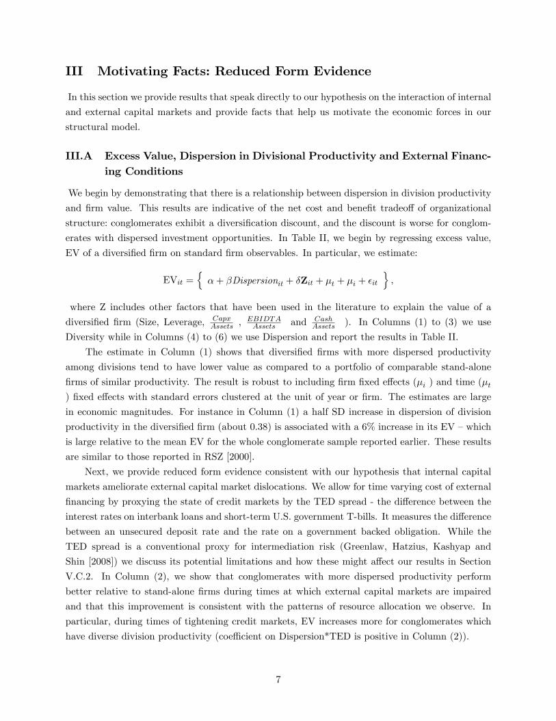
III Motivating Facts: Reduced Form Evidence

In this section we provide results that speak directly to our hypothesis on the interaction of internal

and external capital markets and provide facts that help us motivate the economic forces in our

structural model.

III.A Excess Value, Dispersion in Divisional Productivity and External Financ-ing Conditions

We begin by demonstrating that there is a relationship between dispersion in division productivity

and firm value. This results are indicative of the net cost and benefit tradeoff of organizational

structure: conglomerates exhibit a diversification discount, and the discount is worse for conglom-

erates with dispersed investment opportunities. In Table II, we begin by regressing excess value,

EV of a diversified firm on standard firm observables. In particular, we estimate:

EVit ={α+ βDispersionit + δZit + µt + µi + εit

},

where Z includes other factors that have been used in the literature to explain the value of a

diversified firm (Size, Leverage, CapxAssets ,

EBIDTAAssets and Cash

Assets ). In Columns (1) to (3) we use

Diversity while in Columns (4) to (6) we use Dispersion and report the results in Table II.

The estimate in Column (1) shows that diversified firms with more dispersed productivity

among divisions tend to have lower value as compared to a portfolio of comparable stand-alone

firms of similar productivity. The result is robust to including firm fixed effects (µi ) and time (µt) fixed effects with standard errors clustered at the unit of year or firm. The estimates are large

in economic magnitudes. For instance in Column (1) a half SD increase in dispersion of division

productivity in the diversified firm (about 0.38) is associated with a 6% increase in its EV —which

is large relative to the mean EV for the whole conglomerate sample reported earlier. These results

are similar to those reported in RSZ [2000].

Next, we provide reduced form evidence consistent with our hypothesis that internal capital

markets ameliorate external capital market dislocations. We allow for time varying cost of external

financing by proxying the state of credit markets by the TED spread - the difference between the

interest rates on interbank loans and short-term U.S. government T-bills. It measures the difference

between an unsecured deposit rate and the rate on a government backed obligation. While the

TED spread is a conventional proxy for intermediation risk (Greenlaw, Hatzius, Kashyap and

Shin [2008]) we discuss its potential limitations and how these might affect our results in Section

V.C.2. In Column (2), we show that conglomerates with more dispersed productivity perform

better relative to stand-alone firms during times at which external capital markets are impaired

and that this improvement is consistent with the patterns of resource allocation we observe. In

particular, during times of tightening credit markets, EV increases more for conglomerates which

have diverse division productivity (coeffi cient on Dispersion*TED is positive in Column (2)).

7

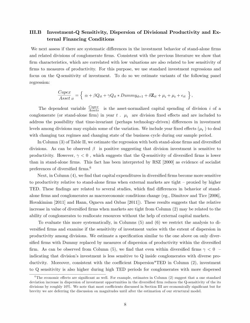
III.B Investment-Q Sensitivity, Dispersion of Divisional Productivity and Ex-ternal Financing Conditions

We next assess if there are systematic differences in the investment behavior of stand-alone firms

and related divisions of conglomerate firms. Consistent with the previous literature we show that

firm characteristics, which are correlated with low valuations are also related to low sensitivity of

firms to measures of productivity. For this purpose, we use standard investment regressions and

focus on the Q-sensitivity of investment. To do so we estimate variants of the following panel

regression:

Capex

Asset it={α+ βQit + γQit ∗Dummyd=1 + δZit + µi + µt + εit

},

The dependent variable CapexAssets is the asset-normalized capital spending of division i of a

conglomerate (or stand-alone firm) in year t . µi are division fixed effects and are included to

address the possibility that time-invariant (perhaps technology-driven) differences in investment

levels among divisions may explain some of the variation. We include year fixed effects (µt ) to deal

with changing tax regimes and changing state of the business cycle during our sample period.

In Column (3) of Table II, we estimate the regression with both stand-alone firms and diversified

divisions. As can be observed β is positive suggesting that division investment is sensitive to

productivity. However, γ < 0 , which suggests that the Q-sensitivity of diversified firms is lower

than in stand-alone firms. This fact has been interpreted by RSZ [2000] as evidence of socialist

preferences of diversified firms.6

Next, in Column (4), we find that capital expenditures in diversified firms become more sensitive

to productivity relative to stand-alone firms when external markets are tight —proxied by higher

TED. These findings are related to several studies, which find differences in behavior of stand-

alone firms and conglomerates as macroeconomic conditions change (eg., Dimitrov and Tice [2006],

Hovakimian [2011] and Hann, Ogneva and Ozbas [2011]). These results suggests that the relative

increase in value of diversified firms when markets are tight from Column (2) may be related to the

ability of conglomerates to reallocate resources without the help of external capital markets.

To evaluate this more systematically, in Columns (5) and (6) we restrict the analysis to di-

versified firms and examine if the sensitivity of investment varies with the extent of dispersion in

productivity among divisions. We estimate a specification similar to the one above on only diver-

sified firms with Dummy replaced by measures of dispersion of productivity within the diversified

firm. As can be observed from Column (5), we find that even within diversified firms γ < 0 —

indicating that division’s investment is less sensitive to Q inside conglomerates with diverse pro-

ductivity. Moreover, consistent with the coeffi cient Dispersion*TED in Column (2), investment

to Q sensitivity is also higher during high TED periods for conglomerates with more dispersed

6The economic effects are significant as well. For example, estimates in Column (2) suggest that a one standarddeviation increase in dispersion of investment opportunities in the diversified firm reduces the Q-sensitivity of the itsdivisions by roughly 10%. We note that most coeffi cients discussed in Section III are economically significant but forbrevity we are deferring the discussion on magnitudes until after the estimation of our structural model.

8

productivity among divisions (Column (3)).

We also use alternative measures of credit supply constraints such as Baa spread and the FED

senior loan offi cer survey to evaluate the robustness of TED and find similar results (unreported for

brevity). Overall, these results suggest that when the cost of external financing is high, the internal

capital market becomes relatively more effi cient, especially in conglomerates with dispersed division

productivity. The likely reason is that conglomerates can reallocate funds internally without the

firm having to incur the cost of raising external funds.

Of course, if Q is mis-measured in a systematic way, either because of issues of measuring pro-

ductivity or endogenous conglomerate composition the estimates presented above will be biased as

well. Further, TED, in addition to measuring variation in credit supply might also capture demand

of conglomerates for funding. As discussed in Section V.C, the major sources of identification in

our structural model are closely related to reduced form evidence presented here. In that section

we discuss why our identification is not affected by measurement error in either productivity or

measures of external capital market frictions. Further, in the Appendix we obtain similar results

as in Table II when we account for potential bias in measured productivity using an oil price based

shifter of dispersion in productivity across divisions of the conglomerate.

This reduced form evidence allows us to track only the net benefit or cost of resource allocation

inside the firm. However, our goal is to identify and quantify the forces driving the reallocation

and how these forces change as the external capital markets change. These quantities are diffi cult

to disentangle from the "net" estimates in reduced form. We are also interested in quantifying how

much of the dislocation in external capital markets is ameliorated by reallocation in internal capital

markets. This is diffi cult to study in reduced form because the crisis data are frequently subject to

other shocks, such as declining productivity and government intervention. As we discuss below, the

structural model allows us to separately identify and quantify the forces driving the reallocation

decision. We can then conduct counterfactuals in which firms are exposed only to shocks in external

capital markets and study how capital reallocates within firms.

IV Theory

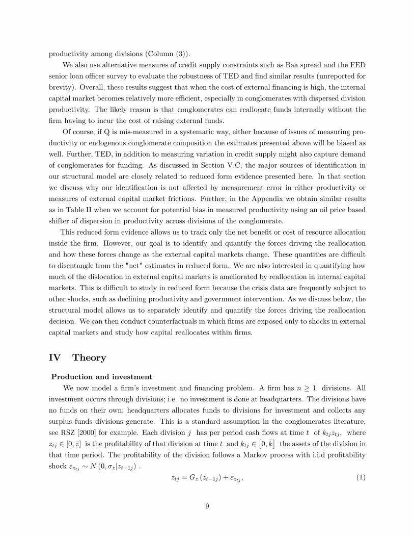
Production and investmentWe now model a firm’s investment and financing problem. A firm has n ≥ 1 divisions. All

investment occurs through divisions; i.e. no investment is done at headquarters. The divisions have

no funds on their own; headquarters allocates funds to divisions for investment and collects any

surplus funds divisions generate. This is a standard assumption in the conglomerates literature,

see RSZ [2000] for example. Each division j has per period cash flows at time t of ktjztj , where

ztj ∈ [0, z] is the profitability of that division at time t and ktj ∈[0, k]the assets of the division in

that time period. The profitability of the division follows a Markov process with i.i.d profitability

shock εztj ∼ N (0, σz|zt−1j) .ztj = Gz (zt−1j) + εztj , (1)

9

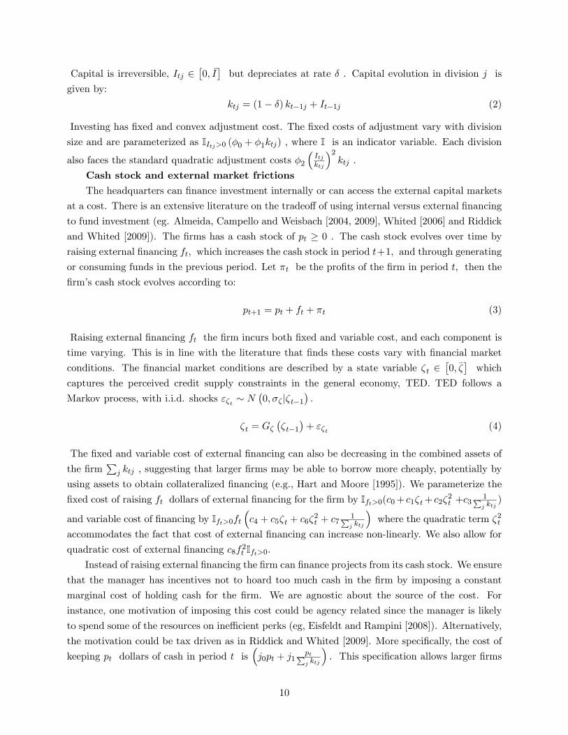
Capital is irreversible, Itj ∈[0, I]but depreciates at rate δ . Capital evolution in division j is

given by:

ktj = (1− δ) kt−1j + It−1j (2)

Investing has fixed and convex adjustment cost. The fixed costs of adjustment vary with division

size and are parameterized as IItj>0 (φ0 + φ1ktj) , where I is an indicator variable. Each division

also faces the standard quadratic adjustment costs φ2(Itjktj

)2ktj .

Cash stock and external market frictionsThe headquarters can finance investment internally or can access the external capital markets

at a cost. There is an extensive literature on the tradeoff of using internal versus external financing

to fund investment (eg. Almeida, Campello and Weisbach [2004, 2009], Whited [2006] and Riddick

and Whited [2009]). The firms has a cash stock of pt ≥ 0 . The cash stock evolves over time by

raising external financing ft, which increases the cash stock in period t+1, and through generating

or consuming funds in the previous period. Let πt be the profits of the firm in period t, then the

firm’s cash stock evolves according to:

pt+1 = pt + ft + πt (3)

Raising external financing ft the firm incurs both fixed and variable cost, and each component is

time varying. This is in line with the literature that finds these costs vary with financial market

conditions. The financial market conditions are described by a state variable ζt ∈[0, ζ]which

captures the perceived credit supply constraints in the general economy, TED. TED follows a

Markov process, with i.i.d. shocks εζt ∼ N(0, σζ |ζt−1

).

ζt = Gζ(ζt−1

)+ εζt (4)

The fixed and variable cost of external financing can also be decreasing in the combined assets of

the firm∑

j ktj , suggesting that larger firms may be able to borrow more cheaply, potentially by

using assets to obtain collateralized financing (e.g., Hart and Moore [1995]). We parameterize the

fixed cost of raising ft dollars of external financing for the firm by Ift>0(c0+ c1ζt+ c2ζ2t +c3

1∑j ktj

)

and variable cost of financing by Ift>0ft(c4 + c5ζt + c6ζ

2t + c7

1∑j ktj

)where the quadratic term ζ2t

accommodates the fact that cost of external financing can increase non-linearly. We also allow for

quadratic cost of external financing c8f2t Ift>0.Instead of raising external financing the firm can finance projects from its cash stock. We ensure

that the manager has incentives not to hoard too much cash in the firm by imposing a constant

marginal cost of holding cash for the firm. We are agnostic about the source of the cost. For

instance, one motivation of imposing this cost could be agency related since the manager is likely

to spend some of the resources on ineffi cient perks (eg, Eisfeldt and Rampini [2008]). Alternatively,

the motivation could be tax driven as in Riddick and Whited [2009]. More specifically, the cost of

keeping pt dollars of cash in period t is(j0pt + j1

pt∑j ktj

). This specification allows larger firms

10

to hold more cash for their day to day operations.

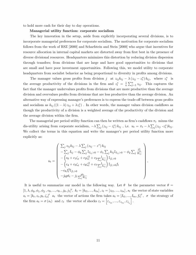
Managerial utility function: corporate socialismThe key innovation in the setup, aside from explicitly incorporating several divisions, is to

incorporate managerial preferences for corporate socialism. The motivation for corporate socialism

follows from the work of RSZ [2000] and Scharfstein and Stein [2000] who argue that incentives for

resource allocation in internal capital markets are distorted away from first best in the presence of

diverse divisional resources. Headquarters minimizes this distortion by reducing division dispersion

through transfers; from divisions that are large and have good opportunities to divisions that

are small and have poor investment opportunities. Following this, we model utility to corporate

headquarters from socialist behavior as being proportional to diversity in profits among divisions.

The manager values gross profits from division j at ztjktj − λ (ztj − z∗t ) ktj , where z∗t is

the average productivity of the divisions in the firm and z∗t = 1n

∑nj=1 ztj . This captures the

fact that the manager undervalues profits from divisions that are more productive than the average

division and overvalues profits from divisions that are less productive than the average division. An

alternative way of expressing manager’s preferences is to express the trade-off between gross profits

and socialism as ktj ((1− λ) ztj + λz∗t ) . In other words, the manager values division cashflows as

though the productivity of a division is a weighted average of the productivity of the division and

the average division within the firm.

The managerial per period utility function can then be written as firm’s cashflows πt minus the

dis-utility arising from corporate socialism, −λ∑

j (ztj − z∗t ) ktj , i,e. ut = πt − λ∑

j(ztj -z∗t )ktj .

We collect the terms in this equation and write the manager’s per period utility function more

explicitly as:

ut =

∑j ztjktj − λ

∑j (ztj − z∗) ktj

−∑

j Itj − φ0∑

j IItj>0 − φ1∑

j ktjIItj>0 − φ2∑

j

I2tjKtj

−(c0 + c1ζt + c2ζ

2t + c3

1∑j ktj

)Ift>0

−(c4 + c5ζt + c6ζ

2t + c7

1∑j ktj

)Ift>0ft

−c8f2t Ift>0−j0ptt − j1 ptt∑

j Ktj

,

It is useful to summarize our model in the following way. Let θ be the parameter vector θ =

[1, λ, φ0, φ1, φ2 , c0, ..., c8, , j0, j1]′, kt = [kt1, ..., ktn] , zt = [zt1, ..., ztn] , st the vector of state variables

st = [kt, zt, pt, ζt]′ at the vector of actions the firm takes at = [It1, ..., Itn, ft]

′ , σ the strategy of

the firm at = σ (st) and εt the vector of shocks εt =[εzt1 , ..., εztn , εζt

].

11

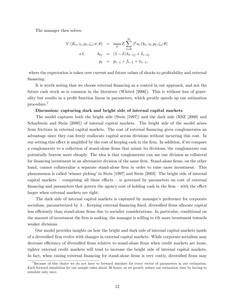
The manager then solves:

V (Kt, zt, pt, ζt;σ; θ) = maxσ

E

∞∑t=0

βtut (kt, zt, pt, ζt; θ)

s.t. ktj = (1− δ) kt−1j + It−1j

pt = pt−1 + ft−1 + πt−1,

where the expectation is taken over current and future values of shocks to profitability and external

financing.

It is worth noting that we choose external financing as a control in our approach, and not the

future cash stock as is common in the literature (Whited [2006]). This is without loss of gener-

ality but results in a profit function linear in parameters, which greatly speeds up our estimation

procedure.7

Discussion: capturing dark and bright side of internal capital marketsThe model captures both the bright side (Stein [1997]) and the dark side (RSZ [2000] and

Scharfstein and Stein [2000]) of internal capital markets. The bright side of the model arises

from frictions in external capital markets. The cost of external financing gives conglomerates an

advantage since they can freely reallocate capital across divisions without incurring this cost. In

our setting this effect is amplified by the cost of keeping cash in the firm. In addition, if we compare

a conglomerate to a collection of stand-alone firms that mimic its divisions, the conglomerate can

potentially borrow more cheaply. The idea is that conglomerate can use one division as collateral

for financing investment in an alternative division of the same firm. Stand-alone firms, on the other

hand, cannot collateralize a separate stand-alone firm in order to raise more investment. This

phenomenon is called ‘winner picking’in Stein [1997] and Stein [2003]. The bright side of internal

capital markets — comprising all these effects — is governed by parameters on cost of external

financing and parameters that govern the agency cost of holding cash in the firm —with the effect

larger when external markets are tight.

The dark side of internal capital markets is captured by manager’s preference for corporate

socialism, parameterized by λ . Keeping external financing fixed, diversified firms allocate capital

less effi ciently than stand-alone firms due to socialist considerations. In particular, conditional on

the amount of investment the firm is making, the manager is willing to tilt more investment towards

weaker divisions.

Our model provides insights on how the bright and dark side of internal capital markets inside

of a diversified firm evolve with changes in external capital markets. While corporate socialism may

decrease effi ciency of diversified firms relative to stand-alone firms when credit markets are loose,

tighter external credit markets will tend to increase the bright side of internal capital markets.

In fact, when raising external financing for stand-alone firms is very costly, diversified firms may

7Because of this choice we do not have to forward simulate for every vector of parameters in our estimation.Each forward simulation for our sample takes about 36 hours, so we greatly reduce our estimation time by having tosimulate only once.

12

allocate capital more effi ciently than stand-alone firms. This suggests that the relative effi ciency

of capital allocation in conglomerates versus stand-alone firms is time varying and depends on the

extent of frictions in external financing and how these frictions interact with socialist motives inside

of diversified firms. In Section V.C we discuss the sources of variation in the data that allow us to

estimate the model and separate these forces.

V Estimation

In this section we describe the estimator that allows us to obtain the parameters of the model

presented in the previous section. We use the two step estimator developed in Bajari et al [2007].8

Because of the large action space of our firm, computing the value function is expensive, and nesting

such an computation in an estimator even more so. This precludes us from applying estimators that

have been commonly used to estimate investment problems (e.g., Hennessy and Whited [2007]). As

we will argue, using the Bajari et al [2007] estimator also provides a tight link to the reduced form

results and allows us to incorporate our instrument for division productivity in a natural way.

The intuition of the Bajari et al [2007] estimator in our problem is the following. The first

stage of the estimation is closely related to the reduced form estimation from Section III. We use

flexible reduced form regressions to estimate the investment and financing choices firms make given

their characteristics. In other words, we estimate the firms’ policy function. We also estimate

the expected evolution of productivity and the TED spread (our state variable for credit supply

constraints) i.e., the state transition function. In the second stage of the estimation we use those

estimates to simulate firms’ expected actions (investment and external financing) and expected

characteristics (capital, amount of cash). For a given set of parameters, the model presented in the

previous section translates firms’expected actions into managers’expected utility.

The estimator then uses the insight that managers’make choices that maximize their expected

utility. In other words, were they to make alternative choices, their utility would be weakly lower. To

implement this insight we create alternative policy functions, i.e. firms choose different investment

and external financing than they do in the data. We then simulate firms’expected actions and

expected characteristics and again use the model (for a given set of parameters) to translate these

into expected utility. We choose the set of parameters that assign the highest expected utility to

the choices that are actually taken by the firms in the data. These parameters are our estimates.

V.A First Stage

V.A.1 Assumptions

In order to be able to recover the policy function from the data using our specifications, Bajari et

al [2007] show that two assumptions need to be satisfied:

8Bajari et al [2007] provide a framework for estimating Markov perfect equilibria of dynamic games. While ourproblem is a decision problem of a firm, not a game, we are faced with the same computational problems that plaguethe dynamic games literature.

13

Assumption MC: ∂2ut∂at∂εt

≥ 0, where ut is our per period managerial utility function. This

assumption is trivially satisfied.

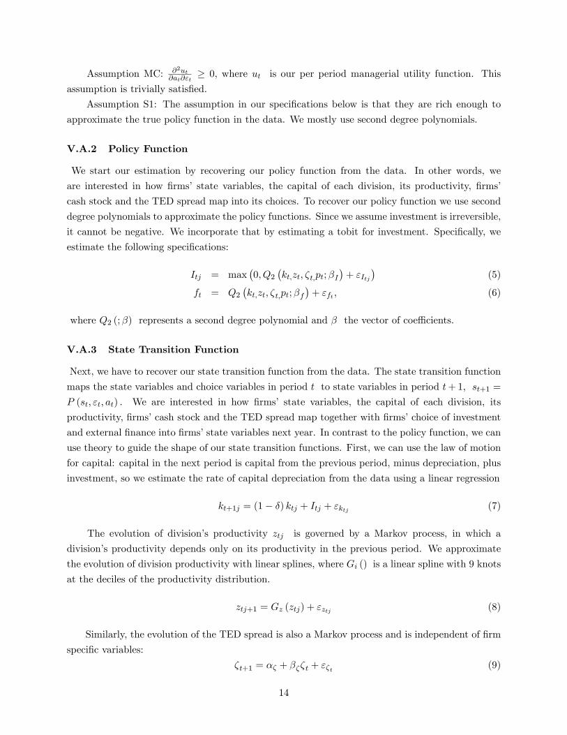
Assumption S1: The assumption in our specifications below is that they are rich enough to

approximate the true policy function in the data. We mostly use second degree polynomials.

V.A.2 Policy Function

We start our estimation by recovering our policy function from the data. In other words, we

are interested in how firms’ state variables, the capital of each division, its productivity, firms’

cash stock and the TED spread map into its choices. To recover our policy function we use second

degree polynomials to approximate the policy functions. Since we assume investment is irreversible,

it cannot be negative. We incorporate that by estimating a tobit for investment. Specifically, we

estimate the following specifications:

Itj = max(0, Q2

(kt,zt, ζt,pt;βI

)+ εItj

)(5)

ft = Q2(kt,zt, ζt,pt;βf

)+ εft , (6)

where Q2 (;β) represents a second degree polynomial and β the vector of coeffi cients.

V.A.3 State Transition Function

Next, we have to recover our state transition function from the data. The state transition function

maps the state variables and choice variables in period t to state variables in period t+ 1, st+1 =

P (st, εt, at) . We are interested in how firms’ state variables, the capital of each division, its

productivity, firms’cash stock and the TED spread map together with firms’choice of investment

and external finance into firms’state variables next year. In contrast to the policy function, we can

use theory to guide the shape of our state transition functions. First, we can use the law of motion

for capital: capital in the next period is capital from the previous period, minus depreciation, plus

investment, so we estimate the rate of capital depreciation from the data using a linear regression

kt+1j = (1− δ) ktj + Itj + εktj (7)

The evolution of division’s productivity ztj is governed by a Markov process, in which a

division’s productivity depends only on its productivity in the previous period. We approximate

the evolution of division productivity with linear splines, where Gi () is a linear spline with 9 knots

at the deciles of the productivity distribution.

ztj+1 = Gz (ztj) + εztj (8)

Similarly, the evolution of the TED spread is also a Markov process and is independent of firm

specific variables:

ζt+1 = αζ + βζζt + εζt (9)

14

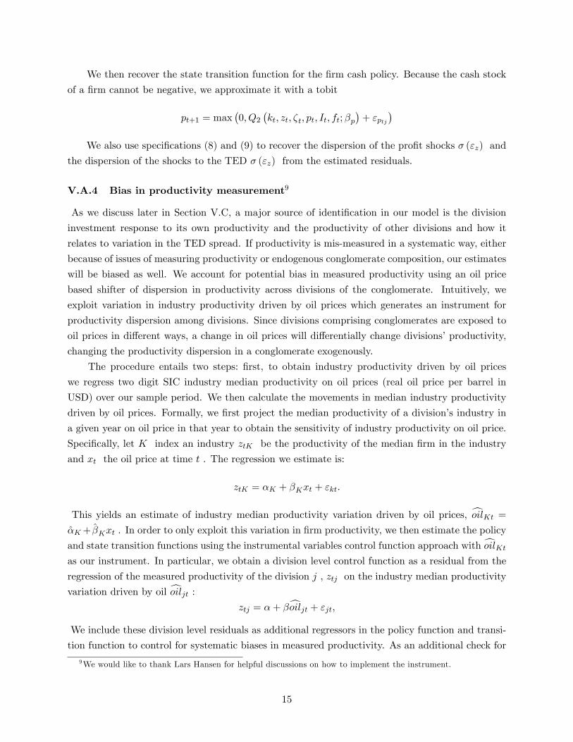
We then recover the state transition function for the firm cash policy. Because the cash stock

of a firm cannot be negative, we approximate it with a tobit

pt+1 = max(0, Q2

(kt, zt, ζt, pt, It, ft;βp

)+ εptj

)We also use specifications (8) and (9) to recover the dispersion of the profit shocks σ (εz) and

the dispersion of the shocks to the TED σ (εz) from the estimated residuals.

V.A.4 Bias in productivity measurement9

As we discuss later in Section V.C, a major source of identification in our model is the division

investment response to its own productivity and the productivity of other divisions and how it

relates to variation in the TED spread. If productivity is mis-measured in a systematic way, either

because of issues of measuring productivity or endogenous conglomerate composition, our estimates

will be biased as well. We account for potential bias in measured productivity using an oil price

based shifter of dispersion in productivity across divisions of the conglomerate. Intuitively, we

exploit variation in industry productivity driven by oil prices which generates an instrument for

productivity dispersion among divisions. Since divisions comprising conglomerates are exposed to

oil prices in different ways, a change in oil prices will differentially change divisions’productivity,

changing the productivity dispersion in a conglomerate exogenously.

The procedure entails two steps: first, to obtain industry productivity driven by oil prices

we regress two digit SIC industry median productivity on oil prices (real oil price per barrel in

USD) over our sample period. We then calculate the movements in median industry productivity

driven by oil prices. Formally, we first project the median productivity of a division’s industry in

a given year on oil price in that year to obtain the sensitivity of industry productivity on oil price.

Specifically, let K index an industry ztK be the productivity of the median firm in the industry

and xt the oil price at time t . The regression we estimate is:

ztK = αK + βKxt + εkt.

This yields an estimate of industry median productivity variation driven by oil prices, oilKt =

αK + βKxt . In order to only exploit this variation in firm productivity, we then estimate the policy

and state transition functions using the instrumental variables control function approach with oilKtas our instrument. In particular, we obtain a division level control function as a residual from the

regression of the measured productivity of the division j , ztj on the industry median productivity

variation driven by oil oiljt :

ztj = α+ βoiljt + εjt,

We include these division level residuals as additional regressors in the policy function and transi-

tion function to control for systematic biases in measured productivity. As an additional check for

9We would like to thank Lars Hansen for helpful discussions on how to implement the instrument.

15

validity of our instrument, we replicate the reduced form regressions discussed in Section III. The

results, reported and discussed in the Appendix, suggest that the instrument is valid.

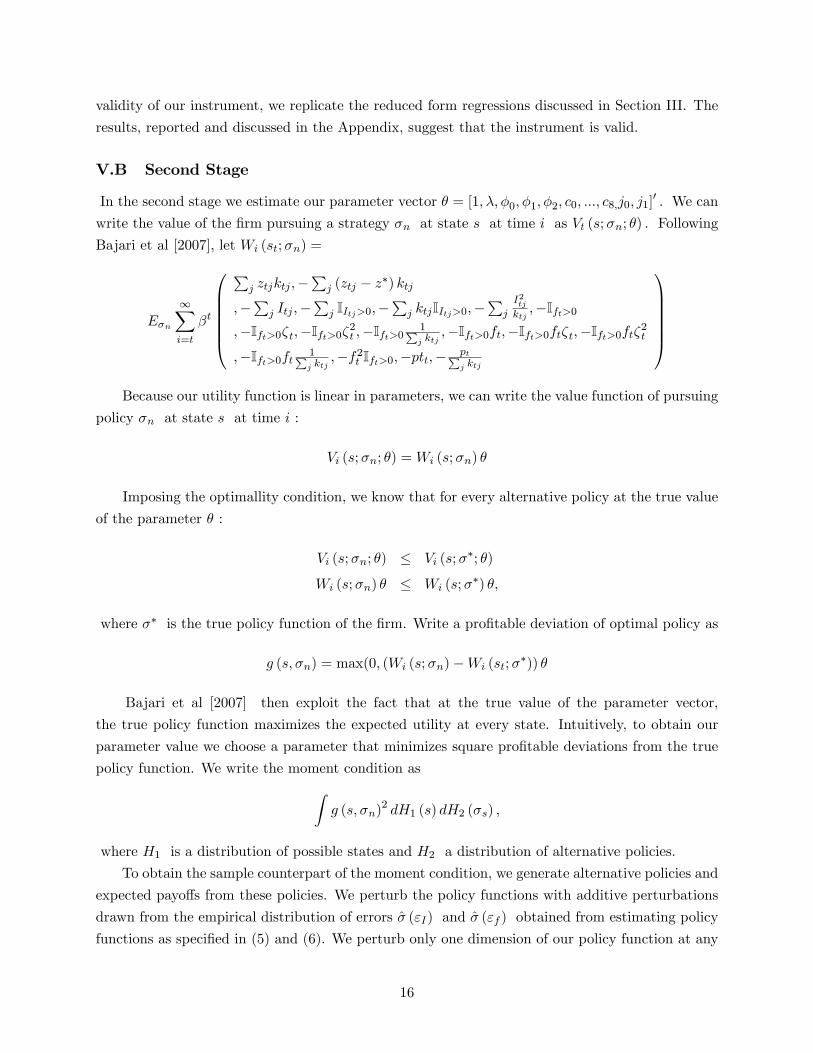
V.B Second Stage

In the second stage we estimate our parameter vector θ = [1, λ, φ0, φ1, φ2, c0, ..., c8,j0, j1]′ . We can

write the value of the firm pursuing a strategy σn at state s at time i as Vt (s;σn; θ) . Following

Bajari et al [2007], let Wi (st;σn) =

Eσn

∞∑i=t

βt

∑

j ztjktj ,−∑

j (ztj − z∗) ktj,−∑

j Itj ,−∑

j IItj>0,−∑

j ktjIItj>0,−∑

j

I2tjktj,−Ift>0

,−Ift>0ζt,−Ift>0ζ2t ,−Ift>0 1∑j ktj

,−Ift>0ft,−Ift>0ftζt,−Ift>0ftζ2t,−Ift>0ft 1∑

j ktj,−f2t Ift>0,−ptt,−

pt∑j ktj

Because our utility function is linear in parameters, we can write the value function of pursuing

policy σn at state s at time i :

Vi (s;σn; θ) = Wi (s;σn) θ

Imposing the optimallity condition, we know that for every alternative policy at the true value

of the parameter θ :

Vi (s;σn; θ) ≤ Vi (s;σ∗; θ)

Wi (s;σn) θ ≤ Wi (s;σ∗) θ,

where σ∗ is the true policy function of the firm. Write a profitable deviation of optimal policy as

g (s, σn) = max(0, (Wi (s;σn)−Wi (st;σ∗)) θ

Bajari et al [2007] then exploit the fact that at the true value of the parameter vector,

the true policy function maximizes the expected utility at every state. Intuitively, to obtain our

parameter value we choose a parameter that minimizes square profitable deviations from the true

policy function. We write the moment condition as∫g (s, σn)2 dH1 (s) dH2 (σs) ,

where H1 is a distribution of possible states and H2 a distribution of alternative policies.

To obtain the sample counterpart of the moment condition, we generate alternative policies and

expected payoffs from these policies. We perturb the policy functions with additive perturbations

drawn from the empirical distribution of errors σ (εI) and σ (εf ) obtained from estimating policy

functions as specified in (5) and (6). We perturb only one dimension of our policy function at any

16

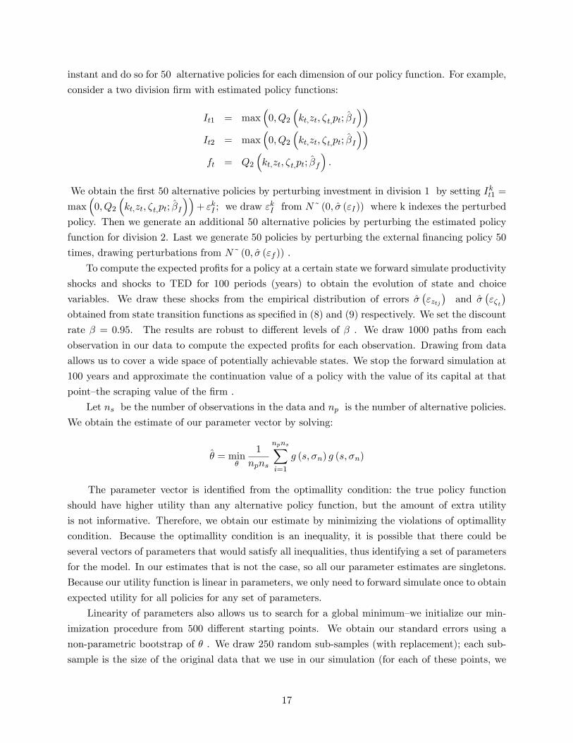
instant and do so for 50 alternative policies for each dimension of our policy function. For example,

consider a two division firm with estimated policy functions:

It1 = max(

0, Q2

(kt,zt, ζt,pt; βI

))It2 = max

(0, Q2

(kt,zt, ζt,pt; βI

))ft = Q2

(kt,zt, ζt,pt; βf

).

We obtain the first 50 alternative policies by perturbing investment in division 1 by setting Ikt1 =

max(

0, Q2

(kt,zt, ζt,pt; βI

))+ εkI ; we draw εkI from N˜ (0, σ (εI)) where k indexes the perturbed

policy. Then we generate an additional 50 alternative policies by perturbing the estimated policy

function for division 2. Last we generate 50 policies by perturbing the external financing policy 50

times, drawing perturbations from N˜ (0, σ (εf )) .

To compute the expected profits for a policy at a certain state we forward simulate productivity

shocks and shocks to TED for 100 periods (years) to obtain the evolution of state and choice

variables. We draw these shocks from the empirical distribution of errors σ(εztj)and σ

(εζt)

obtained from state transition functions as specified in (8) and (9) respectively. We set the discount

rate β = 0.95. The results are robust to different levels of β . We draw 1000 paths from each

observation in our data to compute the expected profits for each observation. Drawing from data

allows us to cover a wide space of potentially achievable states. We stop the forward simulation at

100 years and approximate the continuation value of a policy with the value of its capital at that

point—the scraping value of the firm .

Let ns be the number of observations in the data and np is the number of alternative policies.

We obtain the estimate of our parameter vector by solving:

θ = minθ

1

npns

npns∑i=1

g (s, σn) g (s, σn)

The parameter vector is identified from the optimallity condition: the true policy function

should have higher utility than any alternative policy function, but the amount of extra utility

is not informative. Therefore, we obtain our estimate by minimizing the violations of optimallity

condition. Because the optimallity condition is an inequality, it is possible that there could be

several vectors of parameters that would satisfy all inequalities, thus identifying a set of parameters

for the model. In our estimates that is not the case, so all our parameter estimates are singletons.

Because our utility function is linear in parameters, we only need to forward simulate once to obtain

expected utility for all policies for any set of parameters.

Linearity of parameters also allows us to search for a global minimum—we initialize our min-

imization procedure from 500 different starting points. We obtain our standard errors using a

non-parametric bootstrap of θ . We draw 250 random sub-samples (with replacement); each sub-

sample is the size of the original data that we use in our simulation (for each of these points, we

17

compute all alternative policy functions). As in Bajari et al [2010] and Ryan [2010] these standard

errors do not take into account that the policy function and state transition function are themselves

estimates, and that we compute our expectations with a finite number of simulated paths. As a

result, our standard errors will be slightly biased downwards.

V.C Identification

V.C.1 Sources of variation

Before we proceed to the results from our model it is useful to think about which features in the

data identify the parameters in the model, given the exogenous (instrumented) productivity shocks

and external capital conditions. The identification in the structural model is closely related to the

reduced form estimation from Section III. In the reduced form model, a “too low”responsiveness of

investment to productivity is a sign of miss-allocation. The model uses all coeffi cients from the first

stage regressions simultaneously and interprets “too low”in a quantitative sense using an explicit

production model and expected utility maximization by the manager. While the model is quite

complex, and forces are identified jointly, it is useful to provide some basic tradeoffs and how they

would affect the data.

A large source of identification is the sensitivity of division investment to its own productivity

and the productivity of other divisions. In a frictionless world, the allocation of capital would

be such that the marginal productivity of investment would equal its marginal cost (absent fixed

cost). There are two main sources of frictions in our model which will incorporate the productivity

of one division in the investment decision of the other division. The first is corporate socialism. If

corporate socialism is high, the investment of a division will be higher if other divisions are more

productive. In particular, if a division is more productive than the mean productivity across all

divisions in a firm, it will invest more than it otherwise would, and vice versa. The instrument

allows us to separate this variation from productivity mis-measurement.

The second friction is the cost of raising external capital, which increases the shadow cost of

investing. In contrast to corporate socialism, cost of raising external capital induces investment

in a division to decrease in the productivity of other divisions. Effectively, productivity of other

divisions raises the opportunity cost of investing. To see the intuition, consider the situation in

which a firm is not able to raise any outside financing. With no corporate socialism the optimal

investment equates the marginal return to investing in both divisions. If we can pin down the

cost of external financing, dispersion in productivity across divisions in a firm would identify the

parameter of corporate socialism.

Several features in the data help us pin down cost of external financing and cost of holding

cash, which are interdependent. The first is the response of investment to the level of productivity.

Cost of external financing introduces a wedge between the cost of capital implied by our production

model and the cost of capital faced by the firm; the higher the cost, the larger the wedge. The second

is the responsiveness of external financing to productivity. Were there no cost of external financing,

18

the firm would raise enough external financing to equate the marginal product of investment (given

fixed cost and corporate socialism) to its marginal cost.

Similarly, the firm would pay out all the surplus cash. With cost of external financing and

cost of holding cash, the firm does not raise enough financing and holds a stock of cash. First,

obtaining external financing introduces cost. Further, the firm needs to take into account the cost

of holding cash. It uses the stock of cash to protect itself from incurring cost of external financing

in the future, but holding cash is costly. Therefore if the firm raises too much cash, it will have to

pay the cost of holding it if it does not use it for investment right away. In other words, the higher

the cost of holding cash, the lower is external financing that exceeds current investment needs.

Finally, to identify the time varying component of cost of external financing we exploit the

exogenous variation in TED. The primary source of identification is the correlation of external

financing and TED. However, the cash and investment policies of the firm are also informative,

because they are affected by the time variation in cost of external financing. Holding cash protects

the firm’s ability to invest during temporary spikes in cost of external financing, so how the firm’s

cash stock evolves with TED is also informative on this dimension. Investment also responds to

spikes in external cost of financing, since the firm trades off investing now relative to investing in

the future, when external finance may be easier to access.

V.C.2 Measurement error

The major sources of identification in our model are the division investment response to its own

productivity, the division investment response to productivity dispersion among divisions of a con-

glomerate, and how these investment responses are related to variation in TED spreads. Both our

baseline measure of productivity, Q, and our measure of credit supply constraints, TED, could be

mis-measured in a systematic way, biasing our estimates. For instance, Q could be a poor measure

of productivity. Further, dispersion in Q could be biased because of conglomerate composition.

Finally, TED, in addition to measuring variation in credit supply might also capture demand of

conglomerates for funding. We now discuss the criteria that the measurement error would have to

satisfy in order to generate our results, and argue that such measurement error is highly implausible.

We first construct an alternative measure of productivity to assess the robustness of our esti-

mates to measurement error. As explained below, the alternative measure, return on assets (ROA),

is in fact a natural empirical counterpart to our productivity variable. Even though our findings

are similar using either productivity measure, we use Q as our primary variable. This allows us to

tightly map our findings to the large empirical literature on internal capital markets that also uses

Q as a proxy for productivity. Similarly, we use alternative measures of credit supply constraints

such as Baa spread and the FED senior loan offi cer survey to evaluate the robustness of TED. Of

course, simply using alternative productivity and credit supply measures is not a panacea to all

measurement problems.

While there may be several types of measurement error, the error which may affect our esti-

mation has to be of a specific type. Our model predicts that high productivity divisions have lower

19

investment in conglomerates with more dispersed productivity. Further, during times of high TED,

this effect of dispersion on investments is smaller. Therefore, for measurement error to generate

results in line with our model, the productivity of high productivity divisions has to be systemati-

cally upward biased, this bias has to be larger in conglomerates with more dispersed productivity.

Further, this measurement error has to increase during times of high TED. The converse should

also be true for low productivity divisions.

The same reasoning also suggests that the variation in TED that identifies our model does not

proxy for aggregate credit demand. Our model predicts that if TED measures credit supply, then

the investment sensitivity to productivity of high productivity divisions should increase, and more

so in conglomerates with more dispersed division productivity. The converse would be true for low

productivity divisions. If high TED proxies for low aggregate credit demand it is hard to see how

an increase in TED would induce type of heterogeneous investment response that is predicted by

our model.

Nevertheless, we also address the potential measurement error concerns in two additional

ways. First, we account for potential bias in measured productivity using an oil price based shifter

of dispersion in productivity across divisions of the conglomerate. Since divisions comprising con-

glomerates are in different industries, a change in oil prices will differentially change divisions’

productivity, changing the productivity dispersion in a conglomerate exogenously. If an increase

in oil price increases the productivity dispersion among divisions based on their industry, then our

model predicts that high productivity divisions decrease their sensitivity of investment to produc-

tivity. On the other hand, if an increase in oil prices decreases the productivity dispersion among

divisions based on their industry, then our model predicts that high productivity divisions increase

the sensitivity of investment to productivity. In other words, for measurement error in produc-

tivity to drive our results, once we incorporate the instrument, one would have to believe that an

increase in oil prices drives measurement error exactly in the way our model predicts. Also note

that the investment response to an oil price increase can be positive or negative, depending on the

composition of the conglomerate. Therefore it is hard to generate the results from our model if oil

prices simply proxy for aggregate movements in either demand or supply.

Second, in our counterfactual exercise, we take the estimates from our model during the pre-

crisis period (up to 2006) and simulate firm behavior in the crisis period (2007-2010).10 Even

though this was a very tumultuous period unlike any we have seen since the Great Depression, we

find that the patterns in the actual data during the crisis are remarkably similar to the simulated

data from our model. Again, it is hard to see how our model would predict firm behavior out of

sample in the crisis, if the estimates were driven by some measurement error. For example, it is

hard to see how TED shocks cause heterogenous responses between different types of conglomerates

(in the exact direction predicted by the model) if they proxy for aggregate credit demand.

Taken together these arguments paint a consistent picture. The argument that potential sources

10This approach is similar in spirit to the exercise in Gomes and Livdan [2004] who simulate data using their modeland compare the moments with actual data.

20

of measurement error are generating our estimates faces a very high hurdle. It has to generate very

specific patterns in the data along several dimensions.

VI Empirical Results

In this section we present the results from estimating our model presented in Section IV. We

restrict our attention to conglomerates with two or three divisions, which cover 90 percent of

diversified firms in our sample. We do not have enough data on conglomerates with more than

three divisions to estimate the policy functions with enough precision. Most of our parameters are

estimated statistically significantly at 1 percent.

VI.A Dark Side of Internal Capital Markets

The dark side of internal capital markets in our model arises because of managerial preferences for

corporate socialism. Estimating these preferences is the most novel contribution of this paper—while

there are other estimates of frictions in external capital markets (Hennessy and Whited [2007]), this

is the first paper that provides structural estimates of the distortions in capital allocation between

divisions in a firm. This estimate allow us to quantify the cost of internal capital markets.

Our estimates using Q as a measure of productivity are presented in Panel A of Table III. The

estimate of corporate socialism parameter λ is 0.76 , and is estimated statistically significantly.

As is predicted by the theory (eg. RSZ [2000]), the parameter estimate falls between 0 and 1 ,

suggesting that managers care about equality among divisions’cash-flows, holding all else equal.

Note that since we do not constrain λ to be positive, we could have estimated a negative λ which

would imply that managers prefer excess Darwinism by placing too much weight on divisions with

strong cash-flows.

To illustrate the magnitude of λ, consider a back of the envelope calculation: suppose the firm

has two divisions, and division 1 is γ times as productive as division 2, i.e. z1 = γz2, γ > 1 . The

manager values a dollar of revenues produced by a unit of capital of a division at kizi−λki(zi−z∗)kizi

.

In other words, the manager behaves as though she is maximizing the value of the firm under

the belief that the productivity of the division is a weighted average of division productivity and

average division productivity, (1− λ) zij + λz∗. Therefore, she values the dollar produced at the

more productive division at less than a dollar, at 1 − λ(1− 1

γ

)2 and the less productive division at

more than a dollar at 1 + λ(γ−12

). The average ratio of productivity for two division firms in

our sample is 1.32 . At this dispersion and our estimate of λ, the manager values revenues of the

stronger division at 0.91 and the revenues of the weaker division at 1.12.

Corporate socialism is worse for conglomerates that have more diverse productivity differences

between divisions. To see this more clearly, consider a conglomerate whose productivity ratio is a

standard deviations above the mean at 1.82: the manager values the revenues from the stronger

division at 0.83 and the less productive division at 1.30 . Therefore we show that the manager

21

is willing to tilt more investment towards a weak division, and the tilt can be significant in con-

glomerates with very dispersed productivity. Overall, we estimate significant costs associated with

internal capital markets. In absence of external capital market frictions these estimates reveal the

large advantage of stand-alone firms over conglomerates.

VI.B Bright Side of Internal Capital Markets

The bright side of internal capital markets in our model arises because of frictions in external

capital markets. As discussed before in Section IV, the bright side of internal capital markets is

governed by parameters on cost of external financing and parameters that govern the cost of holding

cash in the firm. We are interested in the average cost of financing, how this cost changes with our

measure of external market conditions, the TED spread, and in ‘winner picking.’

Average cost of financingSince our cost of financing vary with TED, we first evaluate the cost of financing at the average

TED spread in our sample of 0.44 percent. Our estimates imply a fixed cost of financing of 2.4

$mm. This yields mean fixed cost of 3 percent, slightly smaller than the findings of Hennessy and

Whited [2007] for large firms. We also find marginal cost of 12 percent, evaluated at the median

size of a two division firm. These estimates are slightly larger than those found in Hennessy and

Whited [2007] of 8.6 percent. Moreover, consistent with Hennessy and Whited [2007] we also find

little evidence of increasing marginal cost with the size of the issue. While these estimates are

somewhat higher, it is worth noting that they rapidly decline with the size of the firm due to

winner picking as discussed below.

‘Winner picking’Conglomerates have an advantage over stand-alone firms because they can use one division as

collateral for financing investment in an alternative division of the same firm. Stand-alone firms, on

the other hand, cannot collateralize a separate stand-alone firm in order to raise more investment.

This effect is akin to Stein [1997] ‘winner picking’and is parameterized by − (c3 + c7ft)Ift>0∑j ktj

.

To illustrate the magnitude of this benefit consider the following example in the spirit of Stein

[1997] and Stein [2003]. Suppose a conglomerate has two divisions, only one of which has an

investment opportunity. Suppose, also, that the conglomerate has median assets for two division

conglomerates in our sample of 70 $mm, or 35 $mm per division. The conglomerate wants to

raise external financing to finance the profitable investment opportunity at the median amount

in our sample of 14 $mm. We compare this conglomerate to two independent firms, which have

the same productivity and assets as the individual divisions of the conglomerate. However, only

the more productive firm wants to raise financing, since it is the only one with a good investment

opportunity.

The example, while admittedly quite stark, allows us to see the ‘winner picking’effect very

clearly. In particular, the winner picking advantage is computed as the difference between the

financing cost of the conglomerate and the stand-alone. Evaluated at the quantities described above,

the advantage of the conglomerate is(135 −

170

)(c3 + c714) . Our estimates imply a ‘winner picking’

22

advantage of 0.95$mm, or approximately 6.8 percent. While this does represent a substantial

advantage of a conglomerate, the example considered here is quite extreme.

Cost of holding cashOur model imposes a constant marginal cost of holding cash for the firm. We are agnostic

about the source of the cost; it can be agency related or tax driven, as in Riddick and Whited

[2009]. The costs of holding cash is a modeling device that gives managers the incentive to pay-out

funds to suppliers of capital and prevents the firm from hoarding cash. In other words, it allows

the model to rationalize the observed pay-out of capital.

Nevertheless, the magnitude is relevant, since it is related to the shadow cost of cash holdings,

one of the main determinants of the bright side of internal capital markets. The costlier it is to

hold cash, the more valuable is the role of internal capital markets, which can shift capital between

investment opportunities and conserve on holding a large stock of costly cash. Our estimates suggest

that the marginal cost of holding cash is approximately 30 percent. This magnitude rationalizes

the fact that conglomerates frequently pay dividends and conduct share repurchases.

VI.C Effect of time varying credit market conditions

In our model we allow for time varying cost of external financing, where the variation is driven by

changes in the TED spread: as the TED spread increases, so does the cost of accessing the external

capital market.

To illustrate how external financing costs change with the TED spread, we use the estimates

from Panel A of Table III and compute how the total external financing cost increases at the median

amount of external capital in our sample (14 $mm). The quadratic component implies that the

TED shocks affect the cost of external financing in a convex manner. In fact, evaluated at the

median size of external financing, TED values below 1 percent do not change the cost of accessing

external capital markets significantly—staying close to 7 $mm. At a TED of 1.5 percent the cost has

increased to over 12 $mm, and exceeds $25 by the time TED reaches 2 percent. Therefore, when

the external markets are dislocated (high values of TED), only firms with excellent investment

opportunities can justify obtaining external financing to finance projects at hand.

What do these numbers mean? These calculations imply a large shadow value of internal

funds. In other words, having internal funds at disposal has more value when external markets

are dislocated. Since the internal funds can be shifted in internal capital markets relatively more

effi ciently relative to non-integrated firms, these results also suggest that the relative effi ciency of

different organizational forms is time varying. Alternatively put, since the dark and bright sides

of internal capital markets are measured relative to stand-alone firms, these results show that the

conglomerate cost/benefit trade-off is not constant over time but is rather a function of state of the

external capital markets.

In Section VII, we present an alternative way of evaluating the impact of time varying credit

market conditions on allocation of resources inside the firm. We do so by examining a counterfactual

scenario in which we expose firms to external market stress as measured by TED spread spike during

23

the credit market freeze of 2007/2008. In this scenario we study the change in investment behavior

of divisions in a diversified firm relative to a stand-alone firm. The responses of the firm based on

our estimates are then compared to the actual data to evaluate the fit of our model.

VI.D Estimates with an alternative measure of productivity

As discussed earlier, we have so far focused on using Q as a measure of productivity since it

allowed us to compare our estimates to those from the literature. We now conduct additional tests

with an alternative measure of productivity, the return on assets (ROA ), to assess the robustness

of our estimates. In fact, ROA is a natural empirical counterpart to our productivity variable zij .

We compute the ROA of a division in a year as the cash flows of the division in that year divided

by its capital. We obtain cashflows of a division as the sum of the operating cash flow and the

reported accounting depreciation in the year. In the model, a division produces zijkij cash flows

and has assets of kij , so ROA ≈ zijkijkij

= zij .

The results follow a strikingly close pattern as those presented in Panel B of Table III. Specif-

ically, the results yield a similar degree of corporate socialism with λ = 0.69 as compared to 0.76

when Q is used as the measure of productivity in Panel A. Compared to the estimates using Q

as the measure of productivity, we find a higher fixed cost of external financing (9 percent at the

mean level of TED spread) and a smaller marginal cost of financing (of 5 percent), evaluated at

the median size of a two division firm. Other parameters are also qualitatively similar to those

reported in Panel A. Overall, the results in this section provide comfort that the measurement error

in Q is not the likely source of variation driving our estimates.

VII Do firm boundaries mediate financial sector shocks?

We next explore how shocks to the financial sector are mediated by resource allocation inside

diversified firms using our estimated model. We use the recent financial crisis of 2007/2008 to

simulate the disruption in the supply of financial capital and study how shocks to the supply of

capital are propagated differentially through stand-alones and conglomerates. This allows us to

examine the consequences of the credit shock on firm value and how this change in value is related

to the allocation of resources within firms.

VII.A Analysis using simulated data

We start with a random sample of conglomerates and stand-alone firms at the end of 2007 and

expose the firms in the sample to realized values of TED for 2008, 2009 and 2010. We forward

simulate our model by drawing productivity shocks from 2008 and shocks to TED from 2010 onward

for 100 periods. In other words, we conduct our simulation as though the crisis had no effects on firm

productivity, but only affected capital market conditions. We draw 1000 sequences of potential

shock realizations. Note that at any point in time firms’expectations of TED are governed by our

model: a firm in 2008 does not know the realization of TED in 2009, it only forms an expectation

24

given TED in 2008. The realization of TED, however, is the one from the data for 2009. Similarly

for 2009 and 2010. From 2010 onward we simulate possible paths for TED consistent with our

model.

In Panel A of Table IV we present regressions with simulated data. We first examine the

impact of TED shocks on the value of conglomerates relative to stand alone firms, measured by

excess value (EV). We use data based on the forward simulation and define EV as before. In

particular, EV is defined as the log of the ratio of firm value11 of a conglomerate computed relative

to the value of a portfolio of stand-alone firms —with the median stand-alone firm operating in the

same industry as the division of the conglomerate chosen as the comparison firm. In Column (1),

we restrict ourselves to three years around the TED shock. This allows us to make comparisons

with actual data, which is only available from 2007 to 2009. As can be observed, during these years

the relationship between EV and dispersion in productivity is positive. This result is related to the

evidence presented earlier (Table II) where the relationship between EV and Dispersion becomes

less negative during periods of tightened credit markets.

In Figure 2(a) we present the evolution of the diversification discount in our simulations over

time. We find that the conglomerate discount decreases as TED spikes in 2008 but increases when

TED drops in 2009 and 2010. In other words, as external market conditions tighten, conglomerates

become more effi cient relative to stand-alone firms. This pattern emerges in Panel A of Table IV

as well. The relationship between EV and dispersion in division productivity, which was positive in

years around the TED shock (Column 1), changes signs in periods after the TED shock (Column

6).

Next, we explore the source of this increase in relative effi ciency of conglomerates. These firms,

while subject to corporate socialism, are able to direct resources between divisions, while stand-

alone firms are unable to utilize the external capital market to the same effect. In Column (2), we

confirm that this relative value increase of diversified firms is related to the ability of conglomerates

to reallocate resources without the help of external capital markets. In particular, we find that

capital expenditures in diversified firms become more sensitive to productivity relative to stand-

alone firms. In the next three columns we report the relationship between capital expenditures

and productivity for diversified firms only. Column (3) uses data on all the diversified firms in

the sample. Columns (4) and (5) use samples stratified on whether the value of Dispersion for a

conglomerate is above or below median relative to other diversified firms in the sample as of 2007.

The results show that sensitivity of capital expenditures to productivity is higher for conglomerates

with more diverse division productivity.12

We show the same pattern in Figure 2(b): as TED increases in 2008, conglomerates are able

to invest more in high productivity divisions relative to comparable stand-alone firms. Conversely,

Figure 2(c) shows that investment in low productivity divisions in a conglomerate falls in relative

11We compute firm value as the expected present value of cash-flows of the firm across simulated paths. Inparticular, we do not include managerial dis-utility in the calculation of value.12 In unreported tests we find that this increase in investment to Q sensitivity of conglomerates with diverse

investment opportunities is largely driven by divisions with above average investment opportunities.

25

terms over this time period.

VII.B Comparison with real data: Out of sample validation

Even though we estimate the model based on data from 1980 to 2006, the out of sample simula-

tions produce results that are remarkably consistent with the patterns from actual data over the

simulation period of 2007 to 2009. Panel B of Table IV presents these results. We include 2007 as a

baseline pre-crisis year in Panel B, since it represents the starting point for our simulation. There-

fore, by construction, there is no difference between the simulated and actual data in 2007. Note

that this differs from the time period used in simulation results presented in Panel A (post 2007).

Using this data we find that the difference in value of the conglomerate relative to a comparable

portfolio of stand-alone firms decreases as the crisis intensified (coeffi cient DummyY ear=08or09 in

Column (1)). Moreover, the relationship between the excess value of conglomerates and dispersion

in division productivity is positive during the crisis period relative to the period before it.

In addition, this relative increase in the value of diversified firms is related to the ability of con-

glomerates to reallocate resources without the help of external capital markets: capital expenditures

in diversified firms become more sensitive to productivity relative to stand-alone firms (Column

(2)); further, conglomerates with more diverse division productivity have a higher sensitivity of

capital expenditures to productivity (Columns (3) to (5)). In other words, as external market con-

ditions tighten, conglomerates became more effi cient relative to stand-alone firms. These patterns

are also consistent with those found in Kuppuswamy and Villalonga [2010] who use data from 2007

to 2009 and find a decrease in the diversification discount at the beginning of the crisis.

VII.C Discussion

While the counterfactual makes a stark assumption — the crisis was driven solely through an

increase in the cost of accessing external capital markets with firm productivity and investment

opportunities staying at pre-crisis levels —the findings are nevertheless informative on several fronts.

First, as mentioned earlier, the patterns generated by the out of sample simulation are remarkably

consistent with the actual data. Second, these findings again reiterate that corporate socialism in

diversified firms may not be static —it tends to attenuate when the external credit market is tight.

Finally, these findings suggest that an increase in the stress in the financial markets could be

ameliorated by diversified firms through more effi cient resource allocation. The relative value of

an average diversified firm improves from around -21% to -17.5% in the first year after the financial

market dislocation. This amounts to a 16% change in relative valuation. This effect is magnified

for diversified firms with more dispersed division productivity. The effect increases to 30% if we

consider firms in the top quartile based on the dispersion of productivity between divisions.

Of course, the recent financial crisis was not solely driven by a financial market freeze. The crisis

was accompanied by real changes in productivity and large government interventions. Our model

allows us to separate the pure effect of the financial market channel on reallocation decisions from

other contemporaneous effects by comparing the quantitative results from our simulations to the

26

actual data. Our model predicts a smaller increase in EV than was actually realized. It suggests

that of the 5 percentage point increase in the excess value of conglomerates,13 3.5 percentage

points (Figure 2(a)) are due to financial market conditions. Examining reduced form conglomerate

valuations would therefore overstate the extent to which capital reallocation within firms mediates

the effect of financial shocks by up to 30%. Moreover, our simulation suggests that if the crisis were

a pure financial phenomenon, with no changes in productivity, firms would have a higher investment

to Q sensitivity than they actually did during the crisis. This suggests that expectations about

productivity during the crisis did not stay unchanged, as our simulation assumes, but had decreased

from their 2007 levels, which is consistent with evidence in Kahle and Stulz [2010].

VIII Conclusion

We show that improved resource allocation within firms’ internal capital markets provides an

important force countervailing financial market dislocation. We quantify the forces driving the

reallocation decision by estimating a structural model of internal capital markets. This result has

potentially important policy implications. Interventions aimed at de-clogging the banking systems

during recessionary periods, such as during the great recession of 2008-2009, consider the potential

effects on output of firms due to hampered credit. The findings in this paper suggest that unlike

what has been assumed so far in the literature on the credit channel, some firms reallocate resources

internally to significantly mediate the effect of financial shocks. Therefore, these effects may also

be critical to understanding the consequences of policy interventions. This is especially important

in light of the fact that diversified firms comprise large parts of economies around the world.

Our analysis is agnostic about the forces that shape corporate socialism in a firm. It is

reasonable to conjecture that bargaining between top management and outside investors could be

driving part of this effect akin to Scharfstein and Stein [2000]. In addition, it is likely that the

bargaining of divisional managers with the headquarters might also be affecting the extent of tilt

in capital allocation by headquarters. Evaluating whether and how these forces shape the extent

of socialism in a firm is a fruitful area of future research.

More broadly, understanding how firm boundaries mediate financial shocks could be useful in

providing insights on macroeconomic movements. Existing literature suggests that distortions in

resource allocation between firms can have large effects on aggregate TFP (e.g., Bloom [2009]). In

contrast, we study particular sources of distortions to resource allocation- both within and between

firms- and quantify their magnitudes. As a result we provide a new channel through which the

nature of external credit markets may affect the productivity and output of the economy. Our

work suggests that resource allocation within firm boundaries may play a larger role in determining

macro outcomes such as business cycle fluctuations, total factor productivity and ultimately the

path of growth, than has been generally believed.

13To evaluate the change in conglomerate discount during the crisis, we compute the net effect of the 2008 - 2009dummy evaluated at mean dispersion in Column (1), Table IV, Panel B.

27

References

1. Adams, William; Liran, Einav and Levin, Jonathan, (2009), “Liquidity Constraints and

Imperfect Information in Subprime Lending”, American Economic Review, 99, 49-84.

2. Alchian, Armen, (1969), “Corporate Management and Property Rights”, in Henry Manne,

Economic Policy and the Regulation of Corporate Securities, 337-360

3. Almeida, Heitor, Campello, Murillo and Weisbach, Michael, (2004), “The Cash Flow Sensi-

tivity of Cash,”Journal of Finance 59, 1777-1804.

4. Almeida, Heitor, Campello, Murillo and Weisbach, Michael, (2009), “Corporate Financial

and Investment Policies when Future Financing is not Frictionless,” forthcoming Journal of

Corporate Finance.

5. Almeida, Heitor, Campello, Murillo and Hackbarth, Dirk (2011), “Liquidity Mergers”, Forth-

coming, Journal of Financial Economics.

6. Bajari, Patrick; Benkard, Lanier and Levin, Jonathan, (2007), “Estimating Dynamic Models

of Imperfect Competition”, Econometrica, 75.

7. Berger, Philip and Ofek, Eli, (1995), “Diversification’s Effect on Firm Value”, Journal of

Financial Economics, 37, 39-65

8. Bernanke, Ben and Blinder, Alan, (1988), “Money, Credit and Aggregate Demand”, Ameri-

can Economic Review, 78, 435-39.

9. Bernanke, Ben and Blinder, Alan, (1992), “The Federal Funds Rate and the Channels of

Monetary Transmission”, American Economic Review, 82, 901-21.

10. Bernanke, Ben and Gertler, Mark, (1995), “Inside the Black Box: The Credit Channel of

Monetary Policy Transmission”, Journal of Economic Perspectives, 9, 27-48.

11. Bloom, Nicholas, (2009), “The Impact of Uncertainty Shocks”, Econometrica, 77.

12. Bolton, Patrick and Scharfstein, David, (1998), “Corporate Finance, The Theory of The

Firm, and Organizations”, Journal of Economic Perspectives, 12, 95-114

13. Chevalier, Judith, (2004), “What Do We Know about Cross-Subsidization? Evidence from

Merging Firms”, Advances in Economic Analysis and Policy, 4

14. Coase, Ronald, (1937), “The Nature of the Firm”, Economica, 4, 386—405.

15. Dimitrov, Valentin and Sheri Tice, 2006, Corporate diversification and credit constraints:

Real effects across the business cycle, Review of Financial Studies 19, 1465—1498.

28

16. Einav, Liran; Jenkins, Mark and Levin, Joanathan, (2010), “Contract Pricing in Consumer

Credit Markets”, Working Paper.

17. Eisfeldt, Andrea and Rampini, Adriano, (2008), “Managerial Incentives, Capital Realloca-

tion, and the Business Cycle”, Journal of Financial Economics, 177-199.

18. Gomes, Joao, (2001),“Financing Investment”,American Economic Review, 91, 1263-1285.

19. Gomes, Joao and Livdan, Dmitry, (2004), “Optimal Diversification: Reconciling Theory and

Evidence”, The Journal of Finance, 59, 507-535.

20. Greenlaw, David; Hatzius, Jan; Kashyap, Anil and Shin, Hyun, (2008), “Leveraged Losses:

Lessons from the Mortgage Market Meltdown”US Monetary Policy Forum Report No. 2.

21. Hart, Oliver and Moore, John, (1995), “Debt and Seniority: An Analysis of the Role of Hard

Claims in Constraining Management”, American Economic Review, 85, 567-585.

22. Hennessy, Christopher and Whited, Toni, (2007), “How Costly is External Financing? Evi-

dence from a Structural Estimation”, Journal of Finance, 62, 1705-1745.

23. Holmstrom, Bengt and Kaplan, Steven, (2001), “Corporate Governance and Merger Activity

in the U.S.: Making Sense of the 1980s and 1990s”, Journal of Economic Perspectives, 15,

121-144

24. Hovakimian, Gayané, 2011, Financial constraints and investment effi ciency: Internal capital

allocation across the business cycle, Journal of Financial Intermediation 20, 264—283.

25. Imbens, Guido and Newey, Whitney, (2009), “Identification and Estimation of Triangular

Simultaneous Equations Models Without Additivity”Econometrica, 77, 1481-1512.

26. Kahle, Kathleen and Stulz, Rene, (2010), “Financial Policies and the Financial Crisis: How

Important Was the Systemic Credit Contraction for Industrial Corporations?”, Working Pa-

per.

27. Kaplan, Steve and Zingales, Luigi, (1997), “Do Investment-Cashflow Sensitivities Provide

Useful Measures of Financing Constraints?”, Quarterly Journal of Economics, 112, 169-215.

28. Kashyap, Anil and Stein, Jeremy, (2000), “What Do a Million Observations on Banks Say

about the Transmission of Monetary Policy?”, American Economic Review, 90, 407-428.

29. Kuppuswamy, Venkat and Villalonga, Belén, (2010), “Does Diversification Create Value in

the Presence of External Financing Constraints? Evidence from the 2008—2009 Financial

Crisis”, Working Paper.

30. Lang, Larry and Stulz, Rene, (1994), “Tobin’s Q, Corporate Diversification, and Firm Per-

formance”, Journal of Political Economy, 102, 1248-1280.

29

31. Maksimovic, Vojislav and Philips, Gordon, (2002), “Do Conglomerate Firms Allocate Re-

sources Ineffi ciently Across Industries? Theory and Evidence”, Journal of Finance, 57, 721-

767

32. Maksimovic, Vojislav and Philips, Gordon, (2007), “Conglomerate firms and internal capi-

tal markets”, in B. E. Eckbo (Ed.), Handbook of Corporate Finance: Empirical Corporate

Finance, Volume 1, Chapter 8, 423-480

33. Maksimovic, Vojislav and Philips, Gordon, (2008), “The Industry Life Cycle, Acquisitions

and Investment: Does Firm Organization Matter?”, Journal of Finance, 63, 673-708.

34. Ozbas, Oguzhan and Scharfstein, David, (2010), “Evidence on the Dark Side of Internal

Capital Markets”, Review of Financial Studies, Forthcoming

35. Rajan, Raghuram; Servaes, Henry and Zingales, Luigi, (2000), “The Cost of Diversity: The

Diversification Discount and Ineffi cient Investment”, Journal of Finance, 55, 35-80

36. Riddick, Leigh and Whited, Toni, (2009), “The Corporate Propensity to Save”, Journal of

Finance, 64, 1729-1766.

37. Ryan, Stephen, (2010), “The Costs of Environmental Regulation in a Concentrated Indus-

try”, Working Paper.

38. Scharfstein, David and Stein, Jeremy, (2000), “The Dark Side of Internal Capital Markets:

Divisional Rent-Seeking and Ineffi cient Investment”, Journal of Finance, 55, 2537-2564

39. Seru, Amit, (2010), “Firm Boundaries Matter: Evidence from Conglomerates and R&D

Activity”, Journal of Financial Economics, Forthcoming

40. Schoar, Antoinette, (2002), “The Effect of Diversification on Firm Productivity”, Journal of

Finance, 62, 2379-2403

41. Stein, Jeremy, (1997), “Internal Capital Markets and the Competition for Corporate Re-

sources”, Journal of Finance, 52, 111-133

42. Stein, Jeremy (2003) “Agency, Information and Corporate Investment,” in Handbook of

the Economics of Finance, edited by George Constantinides, Milton Harris and René Stulz,

Elsevier 2003, 111-165

43. Villalonga, Belen, (2004), “Does Diversification Cause the Diversification Discount”, Finan-

cial Management, 33, 5-23

44. Whited, Toni, (2001), “Is It Ineffi cient Investment that Causes the Diversification Discount?”,

Journal of Finance, 56, 1667-1692.

45. Whited, Toni, (2006), “External Finance Constraints and the Intertemporal Pattern of In-

termittent Investment”, Journal of Financial Economics, 467-502.

30

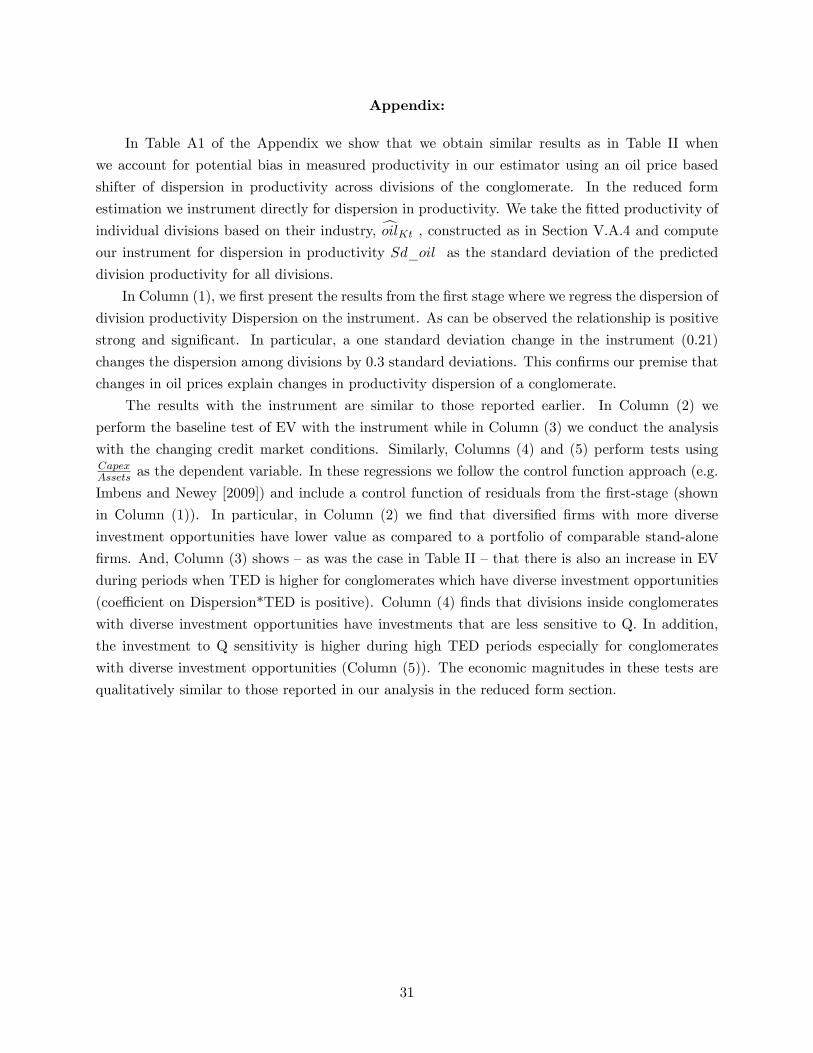
Appendix:

In Table A1 of the Appendix we show that we obtain similar results as in Table II when

we account for potential bias in measured productivity in our estimator using an oil price based

shifter of dispersion in productivity across divisions of the conglomerate. In the reduced form

estimation we instrument directly for dispersion in productivity. We take the fitted productivity of

individual divisions based on their industry, oilKt , constructed as in Section V.A.4 and compute

our instrument for dispersion in productivity Sd_oil as the standard deviation of the predicted

division productivity for all divisions.

In Column (1), we first present the results from the first stage where we regress the dispersion of

division productivity Dispersion on the instrument. As can be observed the relationship is positive

strong and significant. In particular, a one standard deviation change in the instrument (0.21)

changes the dispersion among divisions by 0.3 standard deviations. This confirms our premise that

changes in oil prices explain changes in productivity dispersion of a conglomerate.

The results with the instrument are similar to those reported earlier. In Column (2) we

perform the baseline test of EV with the instrument while in Column (3) we conduct the analysis

with the changing credit market conditions. Similarly, Columns (4) and (5) perform tests usingCapexAssets as the dependent variable. In these regressions we follow the control function approach (e.g.

Imbens and Newey [2009]) and include a control function of residuals from the first-stage (shown

in Column (1)). In particular, in Column (2) we find that diversified firms with more diverse

investment opportunities have lower value as compared to a portfolio of comparable stand-alone

firms. And, Column (3) shows —as was the case in Table II —that there is also an increase in EV

during periods when TED is higher for conglomerates which have diverse investment opportunities

(coeffi cient on Dispersion*TED is positive). Column (4) finds that divisions inside conglomerates

with diverse investment opportunities have investments that are less sensitive to Q. In addition,

the investment to Q sensitivity is higher during high TED periods especially for conglomerates

with diverse investment opportunities (Column (5)). The economic magnitudes in these tests are

qualitatively similar to those reported in our analysis in the reduced form section.

31

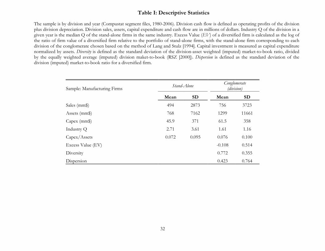
32

Table I: Descriptive Statistics

The sample is by division and year (Compustat segment files, 1980-2006). Division cash flow is defined as operating profits of the division plus division depreciation. Division sales, assets, capital expenditure and cash flow are in millions of dollars. Industry Q of the division in a given year is the median Q of the stand-alone firms in the same industry. Excess Value (EV) of a diversified firm is calculated as the log of the ratio of firm value of a diversified firm relative to the portfolio of stand-alone firms, with the stand-alone firm corresponding to each division of the conglomerate chosen based on the method of Lang and Stulz [1994]. Capital investment is measured as capital expenditure normalized by assets. Diversity is defined as the standard deviation of the division-asset weighted (imputed) market-to-book ratio, divided by the equally weighted average (imputed) division maket-to-book (RSZ [2000]). Dispersion is defined as the standard deviation of the division (imputed) market-to-book ratio for a diversified firm.

Sample: Manufacturing Firms Stand-Alone Conglomerate

(division)

Mean SD

Mean SD

Sales (mm$) 494 2873

756 3723

Assets (mm$) 768 7162

1299 11661

Capex (mm$) 45.9 371

61.5 358

Industry Q 2.71 3.61

1.61 1.16

Capex/Assets 0.072 0.095

0.076 0.100

Excess Value (EV)

-0.108 0.514

Diversity

0.772 0.355

Dispersion

0.423 0.764

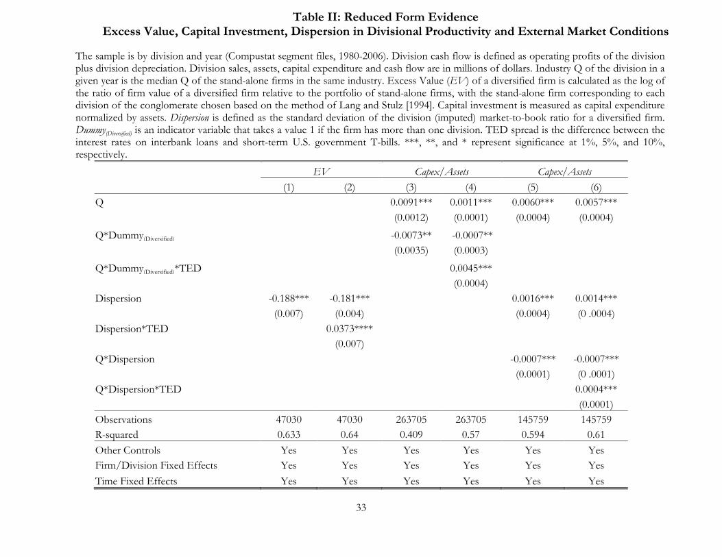
33

Table II: Reduced Form Evidence Excess Value, Capital Investment, Dispersion in Divisional Productivity and External Market Conditions

The sample is by division and year (Compustat segment files, 1980-2006). Division cash flow is defined as operating profits of the division plus division depreciation. Division sales, assets, capital expenditure and cash flow are in millions of dollars. Industry Q of the division in a given year is the median Q of the stand-alone firms in the same industry. Excess Value (EV) of a diversified firm is calculated as the log of the ratio of firm value of a diversified firm relative to the portfolio of stand-alone firms, with the stand-alone firm corresponding to each division of the conglomerate chosen based on the method of Lang and Stulz [1994]. Capital investment is measured as capital expenditure normalized by assets. Dispersion is defined as the standard deviation of the division (imputed) market-to-book ratio for a diversified firm. Dummy(Diversified) is an indicator variable that takes a value 1 if the firm has more than one division. TED spread is the difference between the interest rates on interbank loans and short-term U.S. government T-bills. ***, **, and * represent significance at 1%, 5%, and 10%, respectively.

EV Capex/Assets Capex/Assets (1) (2) (3) (4) (5) (6) Q 0.0091*** 0.0011*** 0.0060*** 0.0057*** (0.0012) (0.0001) (0.0004) (0.0004)

Q*Dummy(Diversified) -0.0073** -0.0007** (0.0035) (0.0003)

Q*Dummy(Diversified)*TED 0.0045*** (0.0004) Dispersion -0.188*** -0.181*** 0.0016*** 0.0014*** (0.007) (0.004) (0.0004) (0 .0004) Dispersion*TED 0.0373**** (0.007) Q*Dispersion -0.0007*** -0.0007*** (0.0001) (0 .0001) Q*Dispersion*TED 0.0004*** (0.0001) Observations 47030 47030 263705 263705 145759 145759 R-squared 0.633 0.64 0.409 0.57 0.594 0.61 Other Controls Yes Yes Yes Yes Yes Yes Firm/Division Fixed Effects Yes Yes Yes Yes Yes Yes Time Fixed Effects Yes Yes Yes Yes Yes Yes

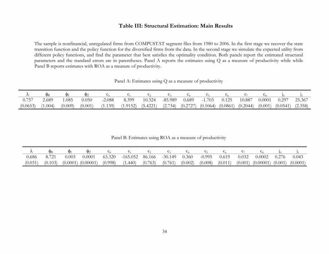
34

Table III: Structural Estimation: Main Results

The sample is nonfinancial, unregulated firms from COMPUSTAT segment files from 1980 to 2006. In the first stage we recover the state transition function and the policy function for the diversified firms from the data. In the second stage we simulate the expected utility from different policy functions, and find the parameter that best satisfies the optimality condition. Both panels report the estimated structural parameters and the standard errors are in parentheses. Panel A reports the estimates using Q as a measure of productivity while while Panel B reports estimates with ROA as a measure of productivity.

Panel A: Estimates using Q as a measure of productivity

λ φ0 φ1 φ2 c0 c1 c2 c3 c4 c5 c6 c7 c8 j0 j1 0.757 2.689 1.085 0.050 -2.088 8.399 10.324 -85.989 0.689 -1.703 0.125 10.887 0.0001 0.297 25.367

(0.0653) (1.004) (0.009) (0.001) (1.139) (1.9152) (5.4221) (2.734) (0.2727) (0.1064) (0.0861) (0.2044) (0.001) (0.0541) (2.358)

Panel B: Estimates using ROA as a measure of productivity

λ φ0 φ1 φ2 c0 c1 c2 c3 c4 c5 c6 c7 c8 j0 j1 0.686 8.721 0.003 0.0001 63.320 -165.052 86.166 -30.149 0.360 -0.995 0.619 0.032 0.0002 0.276 0.043

(0.031) (0.103) (0.0001) (0.00001) (0.998) (1.440) (0.763) (0.761) (0.002) (0.008) (0.011) (0.001) (0.00001) (0.001) (0.0001)

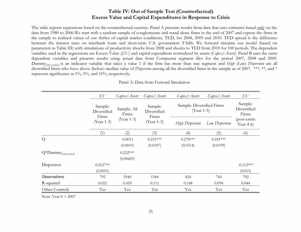
35

Table IV: Out of Sample Test (Counterfactual)

Excess Value and Capital Expenditures in Response to Crisis The table reports regressions based on the counterfactual exercise. Panel A presents results from data that uses estimates based only on the data from 1980 to 2006.We start with a random sample of conglomerate and stand alone firms in the end of 2007 and expose the firms in the sample to realized values of our shifter of capital market conditions, TED, for 2008, 2009 and 2010. TED spread is the difference between the interest rates on interbank loans and short-term U.S. government T-bills. We forward simulate our model (based on parameters in Table III) with simulations of productivity shocks from 2008 and shocks to TED from 2010 for 100 periods. The dependent variables used in the regressions are Excess Value (EV) and capital expenditure normalized by assets (Capex/Assets). Panel B uses the same dependent variables and presents results using actual data from Compustat segment files for the period 2007, 2008 and 2009. Dummy(Diversified) is an indicator variable that takes a value 1 if the firm has more than one segment and High (Low) Dispersion are all diversified firms who have above (below) median value of Dispersion among all the diversified firms in the sample as of 2007. ***, **, and * represent significance at 1%, 5%, and 10%, respectively.

Panel A: Data from Forward Simulation

EV Capex/Assets Capex/Assets Capex/Assets Capex/Assets EV

Sample: Diversified

Firms (Year 1-3)

Sample: All Firms

(Year 1-3)

Sample: Diversified

Firms (Year 1-3)

Sample: Diversified Firms (Year 1-3)

Sample: Diversified

Firms (post-crisis: Year 4-6)

High Dispersion Low Dispersion

(1) (2) (3) (4) (5) (6) Q

-0.0011 0.231*** 0.278*** 0.181***

(0.0019) (0.0187) (0.0314) (0.0199) Q*Dummy(Diversified)

0.232***

(0.00605) Dispersion 0.0127**

-0.112***

(0.0051) (0.015) Observations 792 5940 1584 824 760 792 R-squared 0.052 0.410 0.111 0.148 0.094 0.044 Other Controls Yes Yes Yes Yes Yes Yes Note: Year 0 = 2007

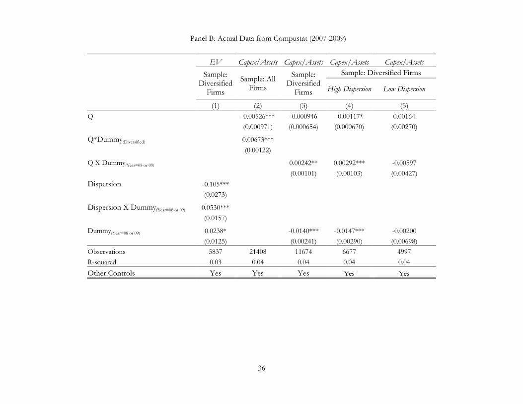
36

Panel B: Actual Data from Compustat (2007-2009)

EV Capex/Assets Capex/Assets Capex/Assets Capex/Assets Sample:

Diversified Firms

Sample: All Firms

Sample: Diversified

Firms

Sample: Diversified Firms

High Dispersion Low Dispersion

(1) (2) (3) (4) (5) Q

-0.00526*** -0.000946 -0.00117* 0.00164

(0.000971) (0.000654) (0.000670) (0.00270)

Q*Dummy(Diversified)

0.00673***

(0.00122)

Q X Dummy(Year=08 or 09)

0.00242** 0.00292*** -0.00597

(0.00101) (0.00103) (0.00427)

Dispersion -0.105***

(0.0273)

Dispersion X Dummy(Year=08 or 09) 0.0530***

(0.0157)

Dummy(Year=08 or 09) 0.0238*

-0.0140*** -0.0147*** -0.00200 (0.0125) (0.00241) (0.00290) (0.00698) Observations 5837 21408 11674 6677 4997 R-squared 0.03 0.04 0.04 0.04 0.04 Other Controls Yes Yes Yes Yes Yes

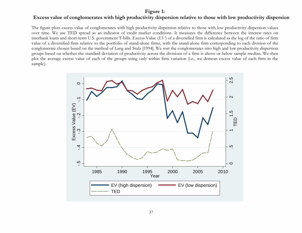
37

Figure 1:

Excess value of conglomerates with high productivity dispersion relative to those with low productivity dispersion The figure plots excess value of conglomerates with high productivity dispersion relative to those with low productivity dispersion values over time. We use TED spread as an indicator of credit market conditions. It measures the difference between the interest rates on interbank loans and short-term U.S. government T-bills. Excess Value (EV) of a diversified firm is calculated as the log of the ratio of firm value of a diversified firm relative to the portfolio of stand-alone firms, with the stand-alone firm corresponding to each division of the conglomerate chosen based on the method of Lang and Stulz [1994]. We sort the conglomerates into high and low productivity dispersion groups based on whether the standard deviation of productivity across the divisions of a firm is above or below sample median. We then plot the average excess value of each of the groups using only within firm variation (i.e., we demean excess value of each firm in the sample).

0.5

11.

52

2.5

TED

0-.1

-.2-.3

-.4-.5

Exc

ess

Val

ue (E

V)

1985 1990 1995 2000 2005 2010Year

EV (high dispersion) EV (low dispersion)TED

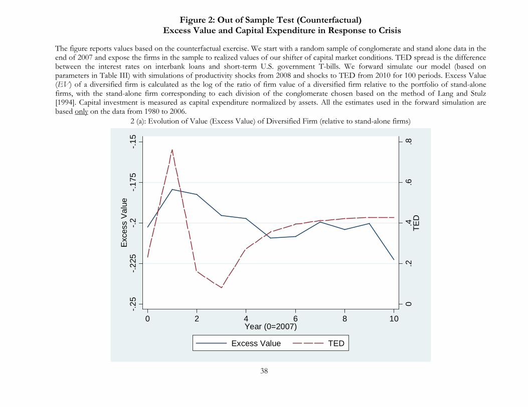
38

Figure 2: Out of Sample Test (Counterfactual)

Excess Value and Capital Expenditure in Response to Crisis The figure reports values based on the counterfactual exercise. We start with a random sample of conglomerate and stand alone data in the end of 2007 and expose the firms in the sample to realized values of our shifter of capital market conditions. TED spread is the difference between the interest rates on interbank loans and short-term U.S. government T-bills. We forward simulate our model (based on parameters in Table III) with simulations of productivity shocks from 2008 and shocks to TED from 2010 for 100 periods. Excess Value (EV) of a diversified firm is calculated as the log of the ratio of firm value of a diversified firm relative to the portfolio of stand-alone firms, with the stand-alone firm corresponding to each division of the conglomerate chosen based on the method of Lang and Stulz [1994]. Capital investment is measured as capital expenditure normalized by assets. All the estimates used in the forward simulation are based only on the data from 1980 to 2006.

2 (a): Evolution of Value (Excess Value) of Diversified Firm (relative to stand-alone firms)

0.2

.4.6

.8TE

D

-.15

-.175

-.2-.2

25-.2

5E

xces

s V

alue

0 2 4 6 8 10Year (0=2007)

Excess Value TED

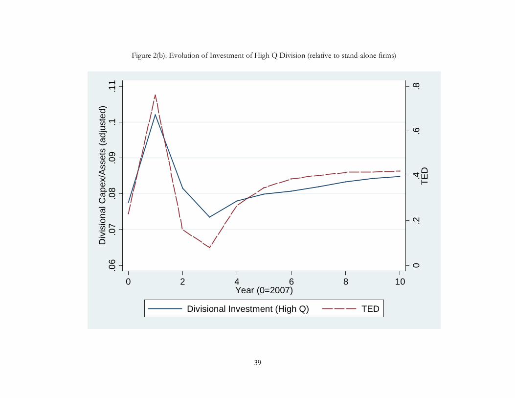
39

Figure 2(b): Evolution of Investment of High Q Division (relative to stand-alone firms)

0.2

.4.6

.8TE

D

.06

.07

.08

.09

.1.1

1D

ivis

iona

l Cap

ex/A

sset

s (a

djus

ted)

0 2 4 6 8 10Year (0=2007)

Divisional Investment (High Q) TED

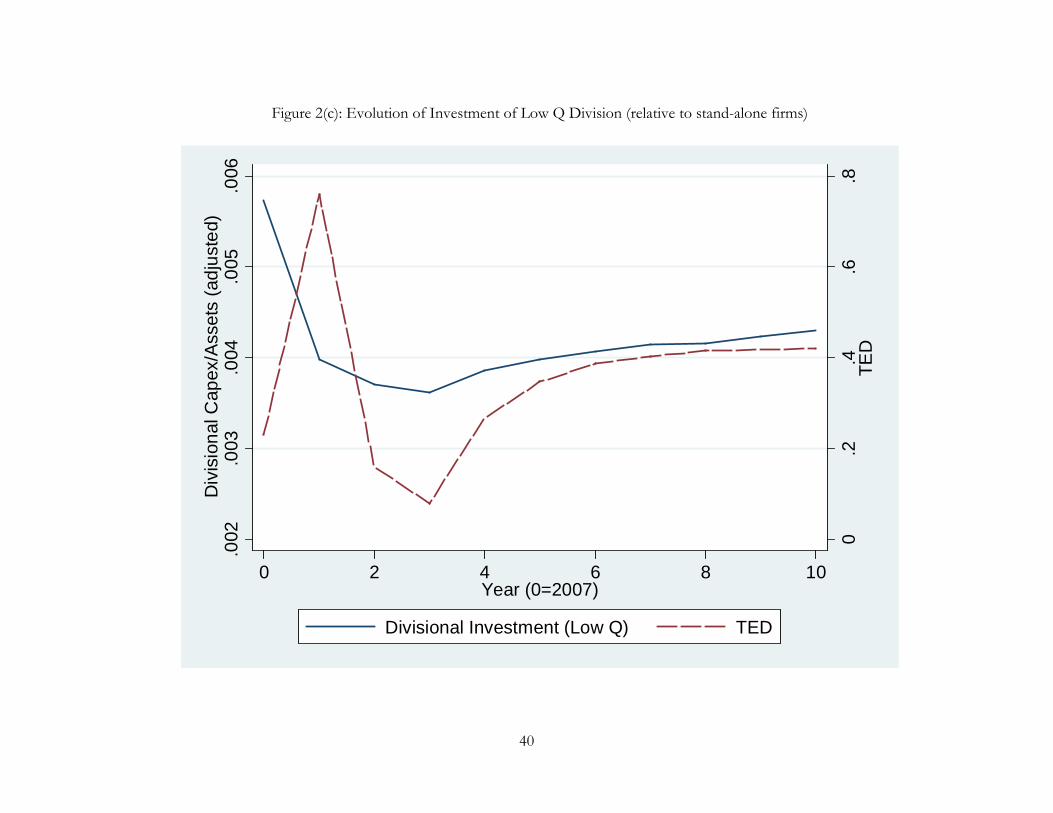
40

Figure 2(c): Evolution of Investment of Low Q Division (relative to stand-alone firms)

0.2

.4.6

.8TE

D

.002

.003

.004

.005

.006

Div

isio

nal C

apex

/Ass

ets

(adj

uste

d)

0 2 4 6 8 10Year (0=2007)

Divisional Investment (Low Q) TED

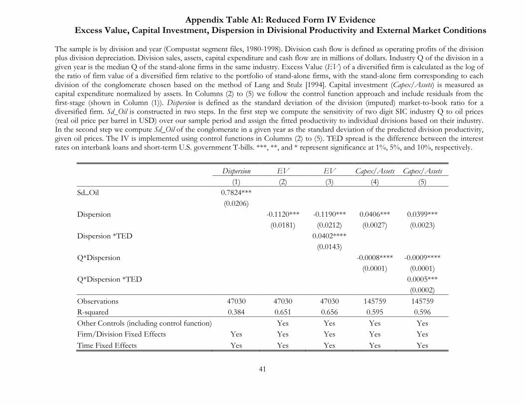
41

Appendix Table A1: Reduced Form IV Evidence

Excess Value, Capital Investment, Dispersion in Divisional Productivity and External Market Conditions The sample is by division and year (Compustat segment files, 1980-1998). Division cash flow is defined as operating profits of the division plus division depreciation. Division sales, assets, capital expenditure and cash flow are in millions of dollars. Industry Q of the division in a given year is the median Q of the stand-alone firms in the same industry. Excess Value (EV) of a diversified firm is calculated as the log of the ratio of firm value of a diversified firm relative to the portfolio of stand-alone firms, with the stand-alone firm corresponding to each division of the conglomerate chosen based on the method of Lang and Stulz [1994]. Capital investment (Capex/Assets) is measured as capital expenditure normalized by assets. In Columns (2) to (5) we follow the control function approach and include residuals from the first-stage (shown in Column (1)). Dispersion is defined as the standard deviation of the division (imputed) market-to-book ratio for a diversified firm. Sd_Oil is constructed in two steps. In the first step we compute the sensitivity of two digit SIC industry Q to oil prices (real oil price per barrel in USD) over our sample period and assign the fitted productivity to individual divisions based on their industry. In the second step we compute Sd_Oil of the conglomerate in a given year as the standard deviation of the predicted division productivity, given oil prices. The IV is implemented using control functions in Columns (2) to (5). TED spread is the difference between the interest rates on interbank loans and short-term U.S. government T-bills. ***, **, and * represent significance at 1%, 5%, and 10%, respectively.

Dispersion EV EV Capex/Assets Capex/Assets

(1) (2) (3) (4) (5) Sd_Oil 0.7824***

(0.0206) Dispersion

-0.1120*** -0.1190*** 0.0406*** 0.0399***

(0.0181) (0.0212) (0.0027) (0.0023)

Dispersion *TED

0.0402****

(0.0143)

Q*Dispersion

-0.0008**** -0.0009****

(0.0001) (0.0001)

Q*Dispersion *TED

0.0005***

(0.0002)

Observations 47030 47030 47030 145759 145759 R-squared 0.384 0.651 0.656 0.595 0.596 Other Controls (including control function)

Yes Yes Yes Yes

Firm/Division Fixed Effects Yes Yes Yes Yes Yes Time Fixed Effects Yes Yes Yes Yes Yes