Regression. Correlation and regression are closely related in use and in math. Correlation...
23
Regression
-
Upload
claud-scott -
Category
Documents
-
view
227 -
download
2
Transcript of Regression. Correlation and regression are closely related in use and in math. Correlation...

Regression
Regression
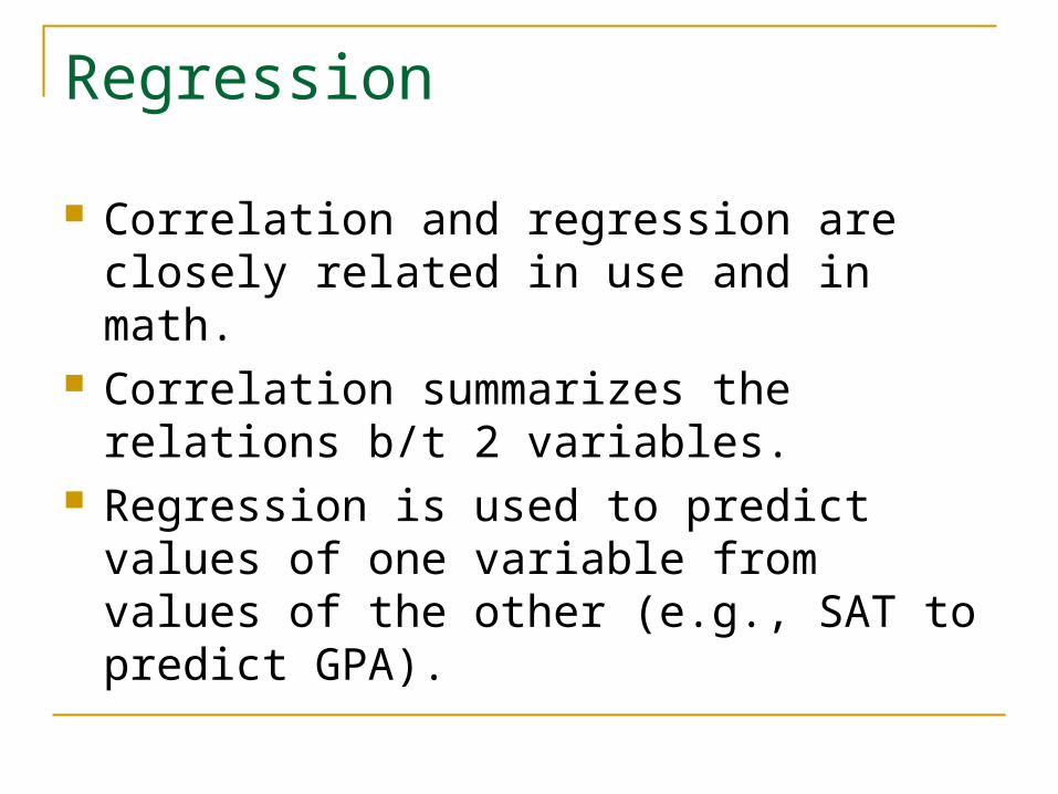
Correlation and regression are closely related in use and in math.
Correlation summarizes the relations b/t 2 variables.
Regression is used to predict values of one variable from values of the other (e.g., SAT to predict GPA).
Basic Ideas (2)
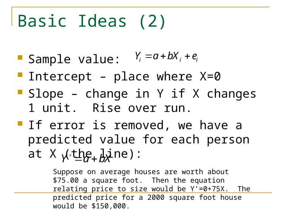
Sample value: Intercept – place where X=0 Slope – change in Y if X changes 1 unit.
Rise over run. If error is removed, we have a predicted
value for each person at X (the line):
Y a bX ei i i
Y a bXSuppose on average houses are worth about $75.00 a square foot. Then the equation relating price to size would be Y’=0+75X. The predicted price for a 2000 square foot house would be $150,000.

Linear Transformation
1 to 1 mapping of variables via line Permissible operations are addition and
multiplication (interval data)
1086420X
40
35
30
25
20
15
10
5
0
Y
Changing the Y Intercept
Y=5+2XY=10+2XY=15+2X
Add a constant
1086420X
30
20
10
0
Y
Changing the Slope
Y=5+.5XY=5+X
Y=5+2X
Multiply by a constant
Y a bX

Linear Transformation (2)
Centigrade to Fahrenheit Note 1 to 1 map Intercept? Slope?
1209060300Degrees C
240
200
160
120
80
40
0D
eg
ree
s F
32 degrees F, 0 degrees C
212 degrees F, 100 degrees C
Intercept is 32. When X (Cent) is 0, Y (Fahr) is 32.
Slope is 1.8. When Cent goes from 0 to 100 (rise), Fahr goes from 32 to 212, and 212-32 = 180. Then 180/100 =1.8 is rise over run is the slope. Y = 32+1.8X. F=32+1.8C.
Y a bX
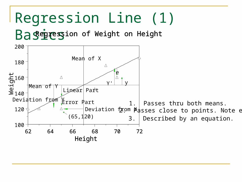
Regression Line (1) Basics
1. Passes thru both means.2. Passes close to points. Note errors.3. Described by an equation.
727068666462Height
200
180
160
140
120
100
We
igh
t
Regression of Weight on Height
727068666462Height
Regression of Weight on Height
Regression of Weight on Height
(65,120)
Mean of X
Mean of Y
Deviation from X
Deviation from Y
Linear Part
Error Part
yY'
e

Regression Line (2) Slope
757269666360
Height
210
180
150
120
90
Wei
ght
Plot of Weight by Height
757269666360
Height
Plot of Weight by Height
Plot of Weight by Height
Mean = 66.8 Inches
Mean = 150.7 lbs.
Second Title
Weight=-327+7.15*Height
Regression line
Equation for a line isY=mX+b in algebra.
In regression, equation usually written Y=a+bX
Y is the DV (weight), X is the IV (height), a is the intercept (-327) and b is the slope (7.15).
The slope, b, indicates rise over run. It tells how many units of change in Y for a 1 unit change in X. In our example, the slope is a bit over 7, so a change of 1 inch is expected to produce a change a bit more than 7 pounds.

Regression Line (3) Intercept
757269666360
Height
210
180
150
120
90
Wei
ght
Plot of Weight by Height
757269666360
Height
Plot of Weight by Height
Plot of Weight by Height
Mean = 66.8 Inches
Mean = 150.7 lbs.
Second Title
Weight=-327+7.15*Height
Regression line
The Y intercept, a, tells where the line crosses the Y axis; it’s the value of Y when X is zero.
The intercept is calculated by: XbYa
Sometimes the intercept has meaning; sometimes not. It depends on the meaning of X=0. In our example, the intercept is –327. This means that if a person were 0 inches tall, we would expect them to weigh –327 lbs. Nonsense. But if X were the number of smiles,then a would have meaning.

Correlation & RegressionCorrelation & regression are closely related.
1. The correlation coefficient is the slope of the regression line if X and Y are measured as z scores. Interpreted as SDY change with a change of 1 SDX.
2. For raw scores, the slope is:
X
Y
SD
SDrb
The slope for raw scores is the correlation times the ratio of 2 standard deviations. (These SDs are computed with (N-1), not N). In our example, the correlation was .96, so the slope can be found by b = .96*(33.95/4.54) = .96*7.45 = 7.15. Recall that . Our intercept is 150.7-7.15*66.8 -327.
XbYa
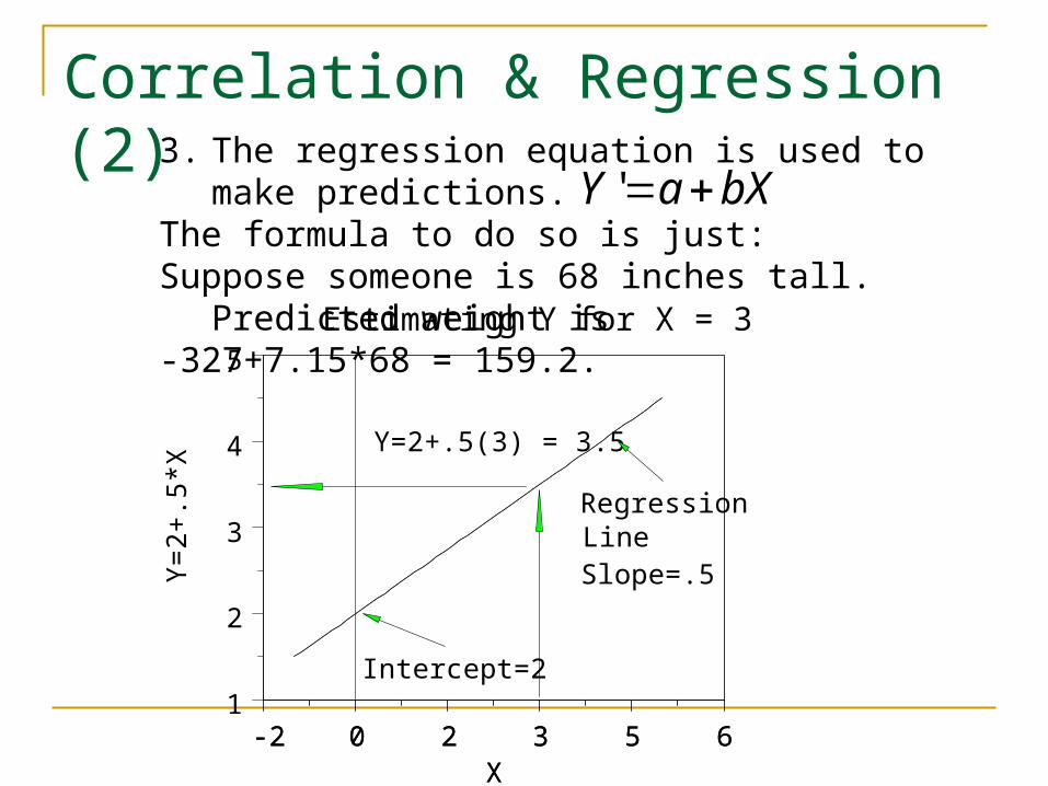
Correlation & Regression (2)3. The regression equation is used to make predictions. The formula to do so is just:Suppose someone is 68 inches tall. Predicted weight is -327+7.15*68 = 159.2.
bXaY '
65320-2X
5
4
3
2
1
Y=
2+
.5*X
65320-2X
Intercept=2
Y=2+.5(3) = 3.5
RegressionLine
Estimating Y for X = 3
Slope=.5
Review
What is the slope? What does it tell or mean?
What is the intercept? What does it tell or mean?
How are the slope of the regression line and the correlation coefficient related?
What is the main use of the regression line?
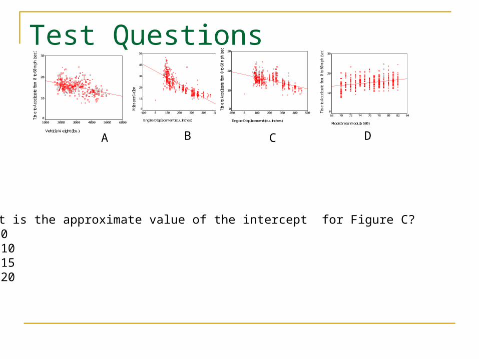
Test Questions
Engine Displacement (cu. inches)
5004003002001000-100
Mile
s pe
r G
allo
n
50
40
30
20
10
0
Engine Displacement (cu. inches)
5004003002001000-100
Tim
e to
Acc
eler
ate fro
m 0
to
60 m
ph (se
c)
30
20
10
0
Model Year (modulo 100)
848280787674727068
Tim
e to
Acc
eler
ate fro
m 0
to
60 m
ph (se
c)
30
20
10
0
Vehicle Weight (lbs.)
600050004000300020001000
Tim
e to
Acc
eler
ate fro
m 0
to
60 m
ph (se
c)
30
20
10
0
A B C D
What is the approximate value of the intercept for Figure C?a. 0b. 10c. 15d. 20
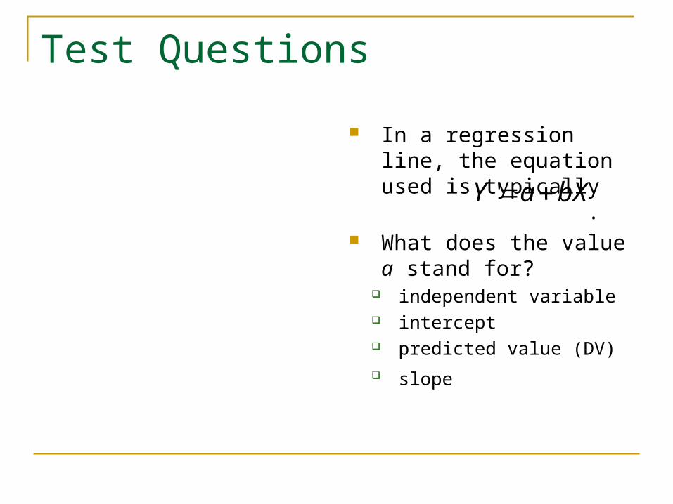
Test Questions
In a regression line, the equation used is typically .
What does the value a stand for?
independent variable intercept predicted value (DV) slope
bXaY '
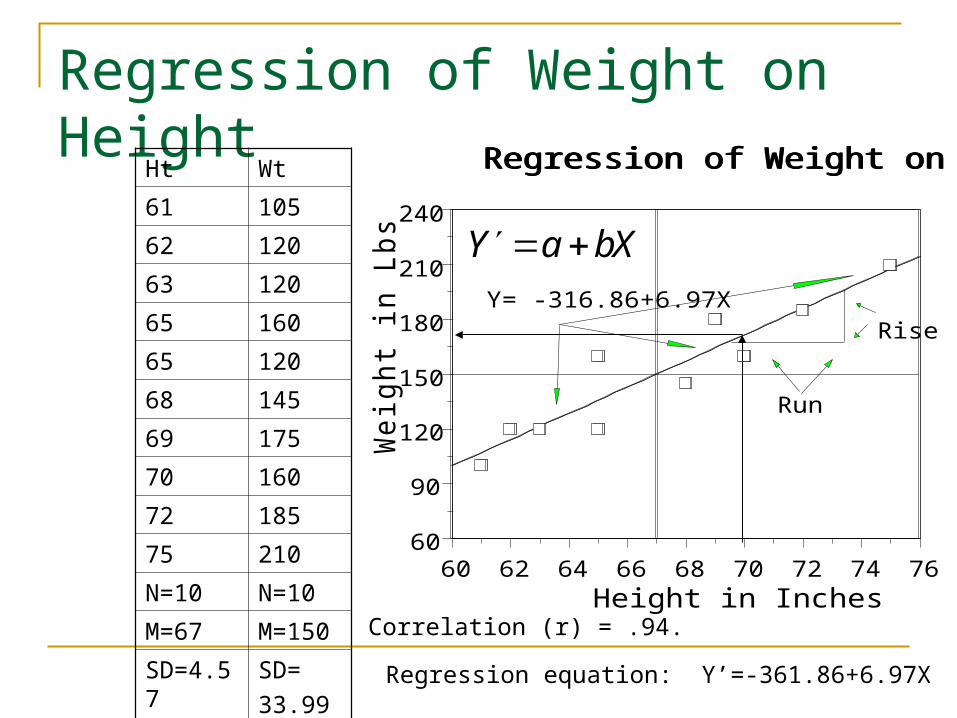
Regression of Weight on Height
Ht Wt
61 105
62 120
63 120
65 160
65 120
68 145
69 175
70 160
72 185
75 210
N=10 N=10
M=67 M=150
SD=4.57 SD=
33.99
767472706866646260Height in Inches
240
210
180
150
120
90
60
We
igh
t in
Lb
s
Regression of Weight on Height
Regression of Weight on Height
Regression of Weight on Height
Rise
Run
Y= -316.86+6.97X
Correlation (r) = .94.
Regression equation: Y’=-361.86+6.97X
Y a bX
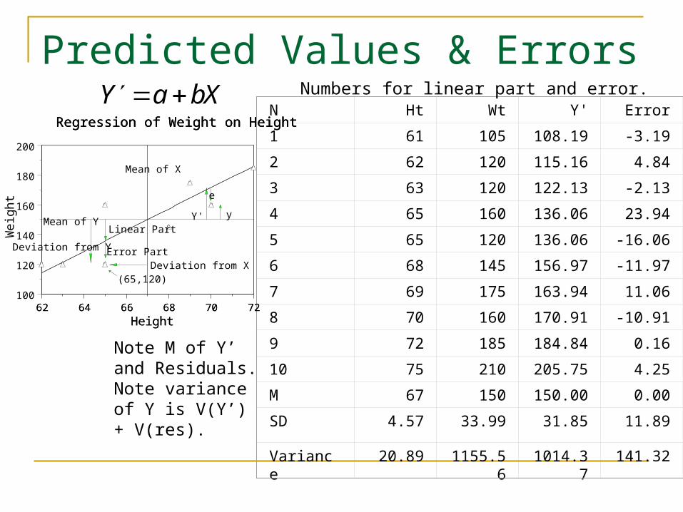
Predicted Values & ErrorsN Ht Wt Y' Error
1 61 105 108.19 -3.19
2 62 120 115.16 4.84
3 63 120 122.13 -2.13
4 65 160 136.06 23.94
5 65 120 136.06 -16.06
6 68 145 156.97 -11.97
7 69 175 163.94 11.06
8 70 160 170.91 -10.91
9 72 185 184.84 0.16
10 75 210 205.75 4.25
M 67 150 150.00 0.00
SD 4.57 33.99 31.85 11.89
Variance 20.89 1155.56 1014.37 141.32
727068666462Height
200
180
160
140
120
100
We
igh
t
Regression of Weight on Height
727068666462Height
Regression of Weight on Height
Regression of Weight on Height
(65,120)
Mean of X
Mean of Y
Deviation from X
Deviation from Y
Linear Part
Error Part
yY'
e
Numbers for linear part and error.
Note M of Y’ and Residuals. Note variance of Y is V(Y’) + V(res).
Y a bX

Error variance
N
YYSY
22
'
)'(
)1( 222' rSS YY
In our example,
88.;94. 2 rr
32.141)'( 2
2'
N
YYSY
141)88.1(*1156)1( 222' rSS YY
Standard error of the Estimate – average distance from prediction
2' 1 rSS YY In our example
1232.141' YS
(Heiman’s notation for error is not standard. )
Variance Accounted for
2
2'2 1Y
Y
S
Sr (Heiman’s notation for
error is not standard. )
The basic idea is to try maximize r-square, the variance accounted for. The closer this value is to 1.0, the more accurate the predictions will be.

Sample Exam Data from Previous Class
86.00 56.0098.00 70.0070.00 76.0084.00 82.0082.00 74.0092.00 94.0092.00 78.0072.00 56.0096.00 66.0082.00 72.00
Exam 1 Exam 2
A sample of 10 scores from both exams
Assuming these are representative, what can you say about the exams? The students?
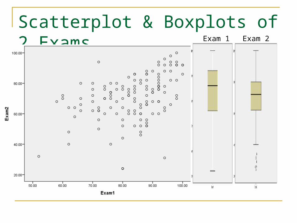
Scatterplot & Boxplots of 2 Exams Exam 1 Exam 2
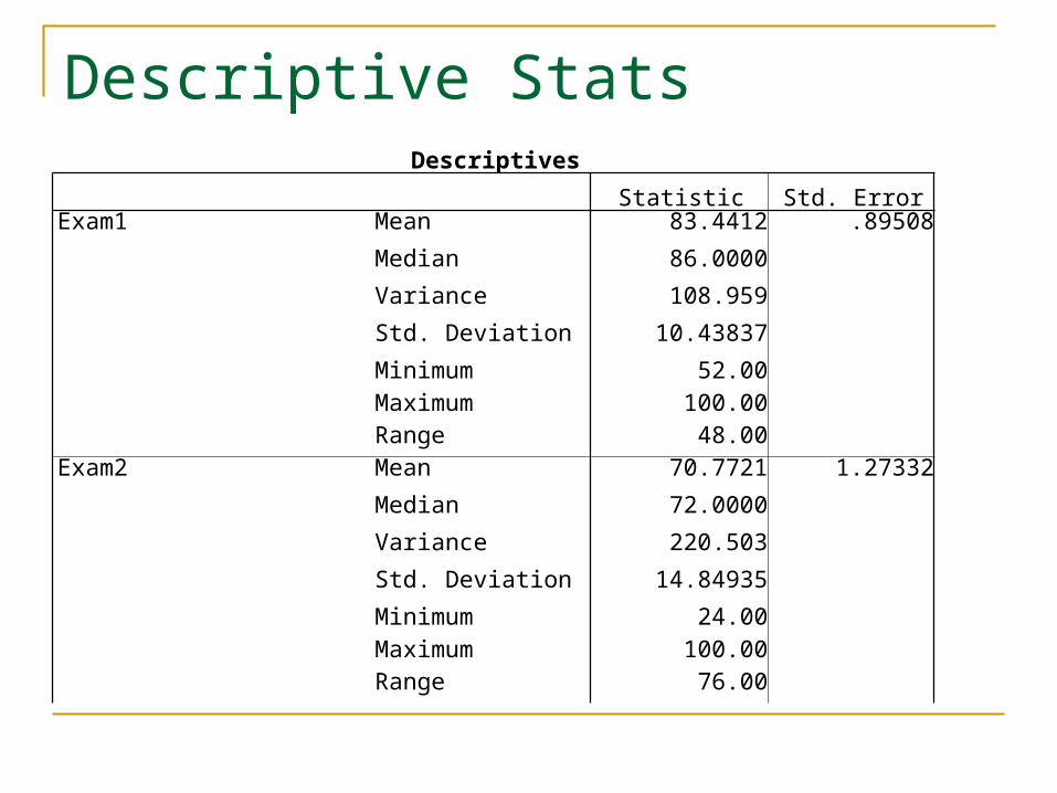
Descriptive StatsDescriptives
Statistic Std. ErrorExam1 Mean 83.4412 .89508
Median 86.0000
Variance 108.959
Std. Deviation 10.43837
Minimum 52.00Maximum 100.00Range 48.00
Exam2 Mean 70.7721 1.27332
Median 72.0000
Variance 220.503
Std. Deviation 14.84935
Minimum 24.00Maximum 100.00Range 76.00
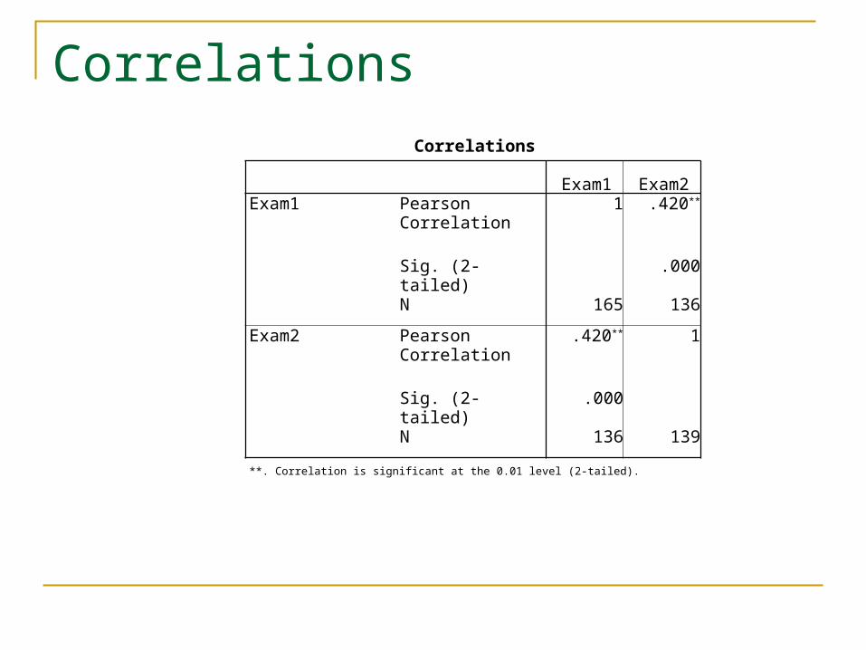
CorrelationsCorrelations
Exam1 Exam2Exam1 Pearson
Correlation1 .420**
Sig. (2-tailed) .000
N 165 136
Exam2 Pearson Correlation
.420** 1
Sig. (2-tailed) .000
N 136 139
**. Correlation is significant at the 0.01 level (2-tailed).

Scatterplot with means and regression line
Coefficientsa
Model
Unstandardized Coefficients
Standardized
Coefficients
t Sig.B Std. Error Beta
1 (Constant) 20.895 9.377 2.228 .028
Exam1 .598 .112 .420 5.360 .000
a. Dependent Variable: Exam2
Note that the correlation, r, is .42 and the squared correlation, R2, is .177. R2 is also the variance accounted for. We can predict a bit less than 20 percent of the variance in Exam 2 from Exam 1.
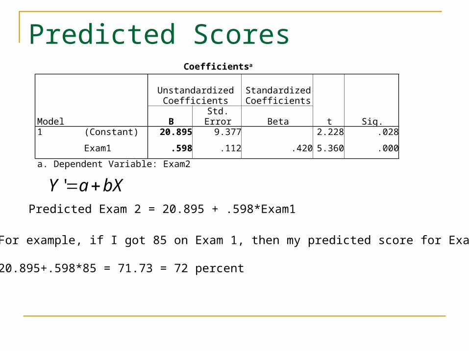
Predicted ScoresCoefficientsa
Model
Unstandardized Coefficients
Standardized Coefficients
t Sig.B Std. Error Beta1 (Constant) 20.895 9.377 2.228 .028
Exam1 .598 .112 .420 5.360 .000
a. Dependent Variable: Exam2
bXaY 'Predicted Exam 2 = 20.895 + .598*Exam1
For example, if I got 85 on Exam 1, then my predicted score for Exam 2 is
20.895+.598*85 = 71.73 = 72 percent