1

Chapter 10

Correlation and Regression

10.2 Correlation

10.3 Regression

2

Consider two variables of a population denoted x and y (e.g. weight and height)

Goal:

Determine if there is a relation between x and y (correlation).

If there is a relation, find a method of predicting values (regression).

Objective

3

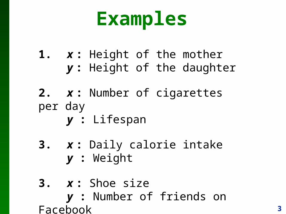
Examples

1. x : Height of the mothery : Height of the daughter

2. x : Number of cigarettes per dayy : Lifespan

3. x : Daily calorie intakey : Weight

3. x : Shoe sizey : Number of friends on Facebook

4

ExampleThis table includes a random sample of heights for mothers and their daughters.

Question

Are the heights of the daughters independent of the heights of the mothers?

Or is there a correlation between them?

If yes, how strong is it?

5

6

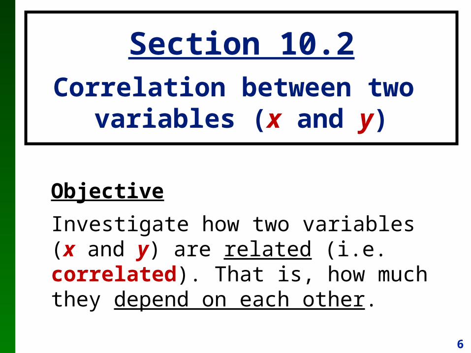
Objective

Investigate how two variables (x and y) are related (i.e. correlated). That is, how much they depend on each other.

Section 10.2Correlation between two

variables (x and y)

7

Definitions

A correlation exists between two variables when the values of one appears to somehow affect the values of the other in some way.

In this class, we are only interested in linear correlation

8

Linear correlation coefficient : rA numerical measure of the strength of the linear relationship between two variables, x and y, representing quantitative data.

r always belongs in the interval (-1,1)

( i.e. –1 r 1 )

We use this value to conclude if there is (or is not) a linear correlation between the two variables.

Definitions

9

Exploring the Data

We can often see a relationship between two variables by constructing a scatterplot.

10

Positive Correlation

We say the data has positive correlation if the data follows a line (with a positive slope).

The correlation coefficient (r) will be close to +1

11

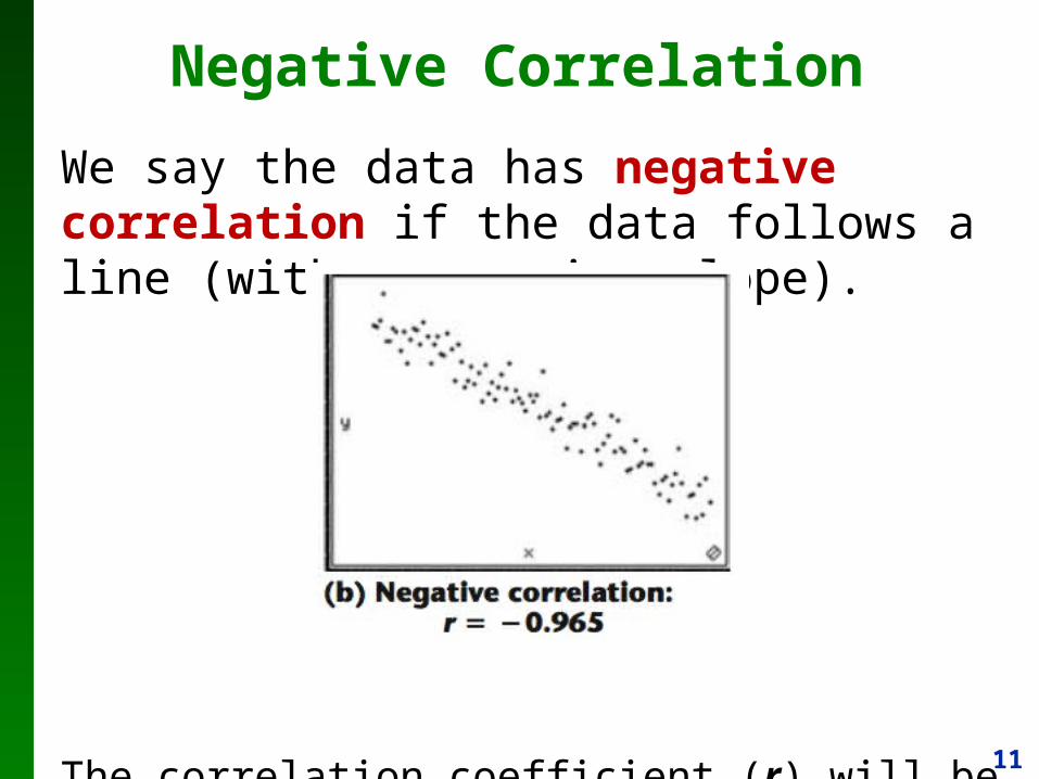
Negative Correlation

We say the data has negative correlation if the data follows a line (with a negative slope).

The correlation coefficient (r) will be close to –1

12

We say the data has no correlation if the data does not seem to follow any line.

The correlation coefficient (r) will be close to 0

No Correlation

13

r ≈ 1 Strong positive linear correlation

r ≈ 0 Weak linear correlation

r ≈ -1 Strong negative linear correlation

Interpreting r

14

Nonlinear Correlation

The data may follow a curve, but if the data is not linear, the linear correlation coefficient (r) will be close to zero.

15

1. The sample of paired (x, y) data is a random sample of quantitative data.

2. Visual examination of the scatterplot must confirm that the points approximate a straight-line pattern.

3. The outliers must be removed if they are known to be errors. (Note: We will not do this in this course)

Requirements

16

r Sample linear correlation coefficient

Population linear correlation coefficient(i.e. the linear correlation between the two populations)

Correlation Coefficient

n(xy) – (x)(y)

n(x2) – (x)2 n(y2) – (y)2r =

r measures the strength of a linear relationship between the paired values in a sample.

We use StatCrunch compute r (Don’t panic!)

17

Round r to three decimal places so that it can be compared to critical values in Table A-6

Rounding the Linear Correlation Coefficient

18

Make a scatterplot for the heights of mother , daughter

1. Enter data on StatCrunch (Mother in 1st column, daughter in 2nd column)

2. Graphics – Scatter Plot Select var1 for X variable (height of mother) Select var2 for Y variable (height of daughter)

3. Click Create Graph!

Example 1a

19

Find the linear correlation coefficient of the heights

Example 1b

The Correlation Coefficient is r = 0.602 (round to 3 decimals)

1. Enter data on StatCrunch (Mother in 1st column, daughter in 2nd column)

2. Stats – Summary Stats – Correlation

3. Select var1 and var2 , then click Calculate

20

Determining if Correlation Exists

We determine whether a population is correlated via a two-tailed test on a sample using a significance level (α)

H0 : ρ = 0 (i.e. not correlated)

H1 : ρ ≠ 0 (i.e. is correlated)

Again, two methods available:

Critical Regions (Use Table A-6)

P-value (Use StatCrunch) Note: In most cases we use significance level = 0.05

21

Use Table A-6 to find the critical values (which depends on the sample size n).

● If the r is in the critical region, we conclude that there is a linear correlation. (reject H0)

● If the r is not in the critical region, there is insufficient evidence of correlation. (fail to reject H0)

Using Critical Regions

-1 10

critical values

22

23

From the mother/daughter data, use a 0.05 significance level to determine if the heights are linearly correlated.

Example 1c

24

From the mother/daughter data, use a 0.05 significance level to determine if the heights are linearly correlated.

Example 1c

Using Critical Regions

● From Example 1b, we found r = 0.602

● Since n = 20 and α = 0.05, using Table A-6, we find the critical values to be: 0.444, -0.444

Since r is in the critical region (reject H0), we conclude the data is linearly correlated (under 0.05 significance).

25

Use StatCrunch to calculate the two-tailed P-value from a sample set (see Example 1c)

● If the P-value is less than α, we conclude that there is a linear correlation.

(Since H0 is rejected)

● If the P-value is greater than α, we say there is insufficient evidence of correlation.

(Since we fail to reject H0)

Using P-value

26

Use a 0.05 significance level to determine if the heights are linearly correlated.

Example 1c

27

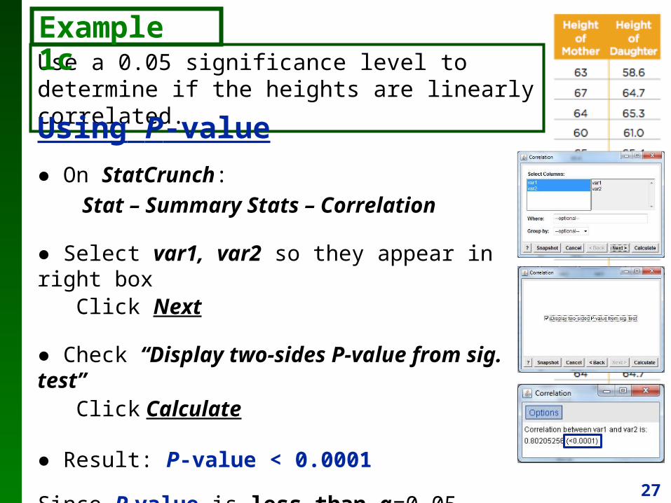
Use a 0.05 significance level to determine if the heights are linearly correlated.

Example 1c

Using P-value

● On StatCrunch:

Stat – Summary Stats – Correlation

● Select var1, var2 so they appear in right box Click Next

● Check “Display two-sides P-value from sig. test” Click Calculate

● Result: P-value < 0.0001

Since P-value is less than α=0.05 (reject H0), we conclude the data is linearly correlated

28

Caution!Know that the methods of this section apply only to a linear correlation.

If you conclude that there is no linear correlation, it is possible that there is some other association that is not linear.

29

Properties of the Linear Correlation Coefficient r

1. –1 r 1

2. If all values of either variable are converted to a different scale, the value of r does not change.

3. The value of r is not affected by the choice of x and y. Interchange all x-values and y-values and the value of r will not change.

4. r measures strength of a linear relationship.

5. r is very sensitive to outliers, they can dramatically affect its value.

30

Interpreting r:Explained Variation

The value of r2 is the proportion of the variation in y that is explained by the linear relationship between x and y.

r = 0.623r 2 = 0.388

r = 0.998r 2 = 0.996

Low variance High variance

31

Common Errors Involving Correlation

1. Causation: It is wrong to conclude that correlation implies causality.

2. Linearity: There may be some relationship between x and y even when there is no linear correlation.

32

Caution!!!Know that correlation does not

imply causality.

There may be correlation without causality.

33

34

Objective

Given two linearly correlated variables (x and y), find the linear function (equation) that best describes the trend.

Section 10.3Regression

35

Equation of a line

Recall that the equation of a line is given by its slope and y-intercept

y = m x + b

36

Regression

For a set of data (with variables x and y) that is linearly correlated, we want to find the equation of the line that best describes the trend.

This process is called Regression

37

x : The predictor variable (Also called the explanatory variable or independent variable)

y : The response variable (Also called the dependent variable)

Regression Equation The equation that describes the algebraically relationship between the two variables

Regression Line The graph of the regression equation (also called the line of best fit or least squares line)

Definitions

38

Regression Equation

y = b0 + b1x

b0 : y-intercept b1 : slope

Regression Line

Definitions

39

Notation for Regression Equation

y-intercept

Slope

Equation

Population

0

1

y = 0 + 1 x

Sample

b0

b1

y = b0 + b1 x

40

1. The sample of paired (x, y) data is a random sample of quantitative data.

2. Visual examination of the scatterplot shows that the points approximate a straight-line pattern.

3. Any outliers must be removed if they are known to be errors. Consider the effects of any outliers that are not known errors.

Requirements

41

Rounding b0 and b1

Round to three significant digits

If you use the formulas from the book, do not round intermediate values.

42

Refer to the sample data given in Table 10-1 in the Chapter Problem.

Find the equation of the regression line in which the explanatory variable (x-variable) is the cost of a slice of pizza and the response variable (y-variable) is the corresponding cost of a subway fare.

(CPI=Consumer Price Index, not used)

Example 1

43

Regression Equation

y = (0.0345) + (0.945)x

Example 1

44

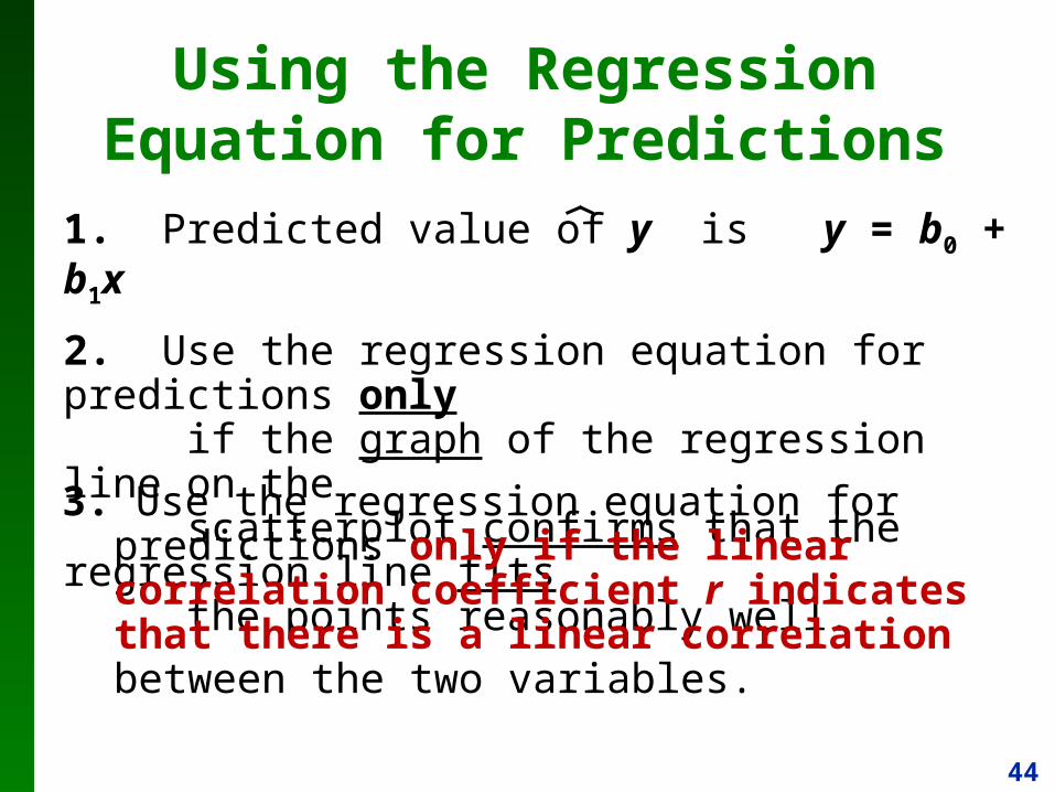
1. Predicted value of y is y = b0 + b1x

2. Use the regression equation for predictions only if the graph of the regression line on the scatterplot confirms that the regression line fits the points reasonably well.

Using the Regression Equation for Predictions

3. Use the regression equation for predictions only if the linear correlation coefficient r indicates that there is a linear correlation between the two variables.

45

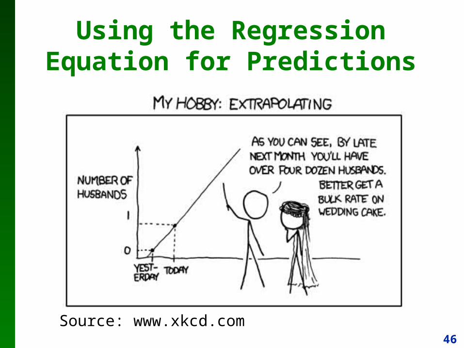
4. Use the regression line for predictions only if the value of x does not go much beyond the scope of the available sample data.

Predicting too far beyond the scope of the available sample data is called extrapolation, and it could result in bad predictions.

Using the Regression Equation for Predictions

5. If the regression equation does not appear to be useful for making predictions, the best predicted value of a variable is its point estimate, which is its sample mean ( y )

_

46

Using the Regression Equation for Predictions

Source: www.xkcd.com

47

Strategy for Predicting Values of Y

48

If the regression equation is not a good model, the best predicted value of y is simply y (the mean of the y values)

Remember, this strategy applies to linear patterns of points in a scatterplot.

Using the Regression Equation for Predictions

_

49

For a pair of sample x and y values, the residual is the difference between the observed sample value of y and the y-value that is predicted by using the regression equation. That is,

Definition

Residual = (observed y) – (predicted y) = y – y

50

Residuals

51

A straight line satisfies the least-squares property if the sum of the squares of the residuals is the smallest sum possible.

The best possible regression line satisfies this properties (hence why it is also called the least squares line)

Definition

52

Least Squares Property

sum = (-5)2 + 112 + (-13) 2 + 72 = 364(any other line would yield a sum larger than 364)