Regression Analysis © 2007 Prentice Hall17-1. © 2007 Prentice Hall17-2 Chapter Outline 1)...

Regression Analysis

© 2007 Prentice Hall 17-1


Chapter Outline1) Correlations

2) Bivariate Regression

3) Statistics Associated with Bivariate Regression

4) Conducting Bivariate Regression Analysis

i. Scatter Diagram

ii. Bivariate Regression Model

iii. Estimation of Parametersiv. Standardized Regression Coefficientv. Significance Testing


Chapter Outline vi. Strength and Significance of Associationvii. Assumptions

5) Multiple Regression

6) Statistics Associated with Multiple Regression

7) Conducting Multiple Regressioni. Partial Regression Coefficientsii. Strength of Associationiii. Significance Testing

8) Multicollinearity

9) Relative Importance of Predictors


Product Moment Correlation

The product moment correlation, r, summarizes the strength of association between two metric (interval or ratio scaled) variables, say X and Y.

It is an index used to determine whether a linear or straight-line relationship exists between X and Y.

r =Cov(X,Y)/SX SY . r varies between -1.0 and +1.0.

The correlation coefficient between two variables will be the same regardless of their underlying units of measurement.


Explaining Attitude Towardthe City of ResidenceTable 17.1

Respondent No Attitude Toward the City

Duration of Residence

Importance Attached to

Weather 1 6 10 3

2 9 12 11

3 8 12 4

4 3 4 1

5 10 12 11

6 4 6 1

7 5 8 7

8 2 2 4

9 11 18 8

10 9 9 10

11 10 17 8

12 2 2 5


Product Moment Correlation

When it is computed for a population rather than a sample, the product moment correlation is denoted by , the Greek letter rho. The coefficient r is an estimator of .

The statistical significance of the relationship between two variables measured by using r can be conveniently tested. The hypotheses are:

H0: = 0H1: 0


Significance of correlation•The test statistic has a t dist with n - 2 degrees of freedom.

•The r bet. ‘Attitude towards city’ and ‘Duration’ is 0.9361

• The value of t-stat is 8.414 and the df = 12-2 = 10. •From the t table (Table 4 in the Stat Appdx), the critical value of t for a two-tailed test and = 0.05 is 2.228.

•Hence, the null hypothesis of no relationship between X and Y is rejected


Partial Correlation

A partial correlation coefficient measures the association between two variables after controlling for, the effects of one or more additional variables.

Partial correlations have an order associated with them. The order indicates how many variables are being adjusted or controlled.


Partial Correlation

The coefficient rxy.z is a first-order partial correlation coefficient, as it controls for the effect of one additional variable, Z.

A second-order partial correlation coefficient controls for the effects of two variables, a third-order for the effects of three variables, and so on.


Regression AnalysisRegression analysis examines associative relationships

between a metric dependent variable and one or more

independent variables in the following ways: Determine whether the independent variables explain a

significant variation in the dependent variable: whether a relationship exists.

Determine how much of the variation in the dependent variable can be explained by the independent variables: strength of the relationship.

Determine the structure or form of the relationship: the mathematical equation relating the independent and dependent variables.

Predict the values of the dependent variable. Control for other independent variables when evaluating

the contributions of a specific variable. Regression analysis is concerned with the nature and

degree of association between variables and does not imply or assume any causality.


Statistics Associated with Bivariate Regression Analysis Regression model. Yi = + Xi + ei whereY

= dep var, X = indep var, = intercept of the line, = slope of the line, and ei is the error term for the i th observation.

Coefficient of determination: r 2. Measures strength of association. Varies bet. 0 and 1 and signifies proportion of the variation in Y accounted for by the variation in X.

Estimated or predicted value of Yi is i = a + bx where i is the predicted value of Yi and a and b are estimators of and

0 1

0 1

Y Y 0 1


Statistics Associated with Bivariate Regression Analysis

Regression coefficient. The estimated parameter b is usually referred to as the non-standardized regression coefficient.

Standard error of estimate. This statistic is the standard deviation of the actual Y values from the predicted values.

Standard error. The standard deviation of b, SEb is called the standard error.

Y


Statistics Associated with Bivariate Regression Analysis Standardized regression coefficient. Also

termed the beta coefficient or beta weight, this is the slope obtained by the regression of Y on X when the data are standardized.

Sum of squared errors. The distances of all the points from the regression line are squared and added together to arrive at the sum of squared errors, which is a measure of total error, .

t statistic. A t statistic with n - 2 degrees of freedom can be used to test the null hypothesis that no linear relationship exists between X and Y

ej 2


Idea Behind Estimating Regression Eqn

A scatter diagram, or scattergram, is a plot of the values of two variables

The most commonly used technique for fitting a straight line to a scattergram is the least-squares procedure.

In fitting the line, the least-squares procedure minimizes the sum of squared errors, . ej 2


Conducting Bivariate Regression Analysis

Fig. 17.2

Plot the Scatter Diagram

Formulate the General Model

Estimate the Parameters

Estimate Standardized Regression Coefficients

Test for Significance

Determine the Strength and Significance of Association


Plot of Attitude with Duration

Fig. 17.3

4.52.25 6.75 11.25 9 13.5

9

3

6

15.75 18

Duration of Residence

Att

itud

e


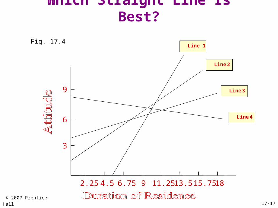
Which Straight Line Is Best?

Fig. 17.4

9

6

3

2.25 4.5 6.75 9 11.25 13.5 15.75 18

Line 1

Line 2

Line 3

Line 4


Decomposing the Total Variation

Fig. 17.6

X2X1 X3 X5X4

Y

X

Total

Variatio

n

SS y

Residual VariationSSres

Explained VariationSSreg

Y


Decomposing the Total Variation

The total variation, SSy, may be decomposed into the variationaccounted for by the regression line, SSreg, and the error or residualvariation, SSerror or SSres, as follows:

SSy = SSreg + SSres

where

S S y = ( Y i - Y ) 2

n i =1

S S r e g = ( Y i - Y ) 2

S S r e s = ( Y i - Y i )

2

n i =1

n i =1


Strength and Significance of Association

Answers the question: ”What percentage of total variation in Y is explained by X?”

R 2 = S S

r e g

S S y

The strength of association is:


Test for Significance

The statistical significance of the linear relationship

between X and Y may be tested by examining thehypotheses:

A t statistic with n - 2 degrees of freedom can beused, where

SEb denotes the standard deviation of b and is called

the standard error.

H0: 1 = 0H1: 10

t = bSEb


Standardization is the process by which the raw data are transformed into new variables having a mean of 0 and a variance of 1

When the data are standardized, the intercept assumes a value of 0.

The term beta coefficient or beta weight is used to denote the standardized regression coefficient, Byx

There is a simple relationship between the standardized and non-standardized regression coefficients:

Byx = byx (Sx /Sy)

Standardized Regression Coefficient


Illustration of Bivariate Regression

The regression of attitude on duration of residence, using the data shown in Table 17.1, yielded the results shown in Table 17.2. a= 1.0793, b= 0.5897. The estimated equation is:

Attitude ( ) = 1.0793 + 0.5897 (Duration of residence)

The standard error, or standard deviation of b is 0.07008, and

t = 0.5897/0.0700 =8.414, with n - 2 = 10 df.

From Table 4 in the Statistical Appendix, we see that the criticalvalue of t with 10 df and = 0.05 is 2.228. Since the calculated value of t is larger than the critical value, the null hypothesis is rejected.

Y


Bivariate RegressionTable 17.2

Multiple R 0.93608R2 0.87624Adjusted R2 0.86387Standard Error 1.22329

ANALYSIS OF VARIANCEdf Sum of SquaresMean Square

Regression 1 105.95222 105.95222Residual 10 14.96444 1.49644F = 70.80266 Significance of F = 0.0000

VARIABLES IN THE EQUATIONVariable b SEb Beta (ß) T Significance of TDuration 0.58972 0.07008 0.936088.414 0.0000(Constant) 1.07932 0.74335 1.452 0.1772



The predicted values ( ) can be calculated using Attitude ( ) = 1.0793 + 0.5897 (Duration of residence)

For the first observation in Table 17.1, this value is: = 1.0793 + 0.5897 x 10 = 6.9763. For each observation, we can obtain this value Using these,

=105.9524,

=14.9644

R2 =105.95/(105.95+14.96)=0.8762,

Y

Y

Y

SSreg

= (Yi

- Y )2

i=1

n

SSres = (Y i - Y i)2

i=1

n



Another, equivalent test for examining the significance of the linear relationship between X and Y (significance of b) is the test for the significance of the coefficient of determination. The hypotheses in this case are:

H0: R2

pop = 0

H1: R2

pop > 0



The appropriate test statistic is the F statistic:

which has an F distribution with 1 and n - 2 degrees of freedom. The F test for testing the significance of the coefficient of determination is equivalent to testing the following hypotheses:

or

F = SSreg

SSres/(n-2)

H0: 1 = 0

H0: 10

H0: = 0H0: 0



From Table 17.2, it can be seen that: r2 = 105.9522/(105.9522 + 14.9644) = 0.8762 The value of the F statistic is: F = 105.9522/(14.9644/10) = 70.8027 with 1 and 10 degrees of freedom. The calculated F statisticexceeds the critical value of 4.96 determined from Table 5 in

theStatistical Appendix. Therefore, the relationship is significant

at = 0.05, corroborating the results of the t test.


Assumptions

The error term is normally distributed. For each fixed value of X, the distribution of Y is normal.

The means of all these normal distributions of Y, given X, lie on a straight line with slope b.

The mean of the error term is 0.

The variance of the error term is constant. This variance does not depend on the values assumed by X.

The error terms are uncorrelated. In other words, the observations have been drawn independently.


Multiple Regression

The general form of the multiple regression model

is as follows:

which is estimated by the following equation:

= a + b1X1 + b2X2 + b3X3+ . . . + bkXk

As before, the coefficient a represents the intercept,but the b's are now the partial regression

coefficients.

Y

Y = 0 + 1X1 + 2X2 + 3 X3+ . . . + k Xk + ee


Stats Associated with Multiple Reg

Coefficient of multiple determination. The strength of association is measured by R2.

Adjusted R2. R2, coefficient of multiple determination, is adjusted for the number of independent variables and the sample size.

F test. The F test is used to test the null hypothesis that the coefficient of multiple determination in the population, R2

pop, is zero. The test statistic has an F distribution with k and (n - k - 1) degrees of freedom.


Stats Associated with Multiple Reg Partial regression coefficient. The partial

regression coefficient, b1, denotes the change in the predicted value, , per unit change in X1 when the other independent variables, X2 to Xk, are held constant.

Suppose one was to remove the effect of X2 from X1. This could be done by running a regression of X1 on X2. In other words, one would estimate the equation 1 = a + b X2 and calculate the residual Xr = (X1 - 1). The partial regression coefficient, b1, is then equal to the bivariate regression coefficient, br , obtained from the equation = a + br Xr .

Y

X

X

Y


The Multiple Regression Equation For data in Table 17.1, suppose we want

to explain ‘Attitude Towards City’ by ‘Duration’ and ‘Importance of Weather’

From Table 17.3, the estimated regression equation is:

( ) = 0.33732 + 0.48108 X1 + 0.28865 X2

orAttitude = 0.33732 + 0.48108 (Duration) +

0.28865 (Importance)

Y


Multiple RegressionTable 17.3

Multiple R 0.97210R2 0.94498Adjusted R2 0.93276Standard Error 0.85974

ANALYSIS OF VARIANCEdf Sum of SquaresMean Square

Regression 2 114.26425 57.13213 Residual 9 6.65241 0.73916 F = 77.29364 Significance of F = 0.0000

VARIABLES IN THE EQUATIONVariable b SEb Beta (ß) T Significance of TIMPORTANCE 0.28865 0.08608 0.31382 3.353 0.0085 DURATION 0.48108 0.05895 0.76363 8.160 0.0000 (Constant) 0.33732 0.56736 0.595 0.5668


Strength of Association

The strength of association is measured by R2, which is similar to bivariate case

R 2 = SS reg

SSy

R2 is adjusted for the number of independent variables and the sample size by using the following formula:

Adjusted R2 = R 2 - k(1 - R 2)n - k - 1


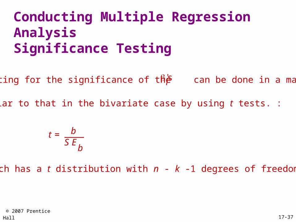
Conducting Multiple Regression AnalysisSignificance Testing

H0 : R2pop = 0

This is equivalent to the following null hypothesis:

H0: 1 = 2 = 3 = . . . = k = 0

The overall test can be conducted by using an F statistic:

F = SSreg/k

SSres/(n - k - 1)

= R 2/k(1 - R 2)/(n- k - 1)

which has an F distribution with k and (n - k -1) degrees of freedom.


Testing for the significance of the can be done in a manner i's

similar to that in the bivariate case by using t tests. :

t = bS E

b

which has a t distribution with n - k -1 degrees of freedom.

Conducting Multiple Regression AnalysisSignificance Testing


A residual is the difference between the observed value of Yi and the value predicted by the regression equation i.

Scattergrams of the residuals, in which the residuals are plotted against the predicted values, i, time, or predictor variables, provide useful insights in examining the appropriateness of the underlying assumptions and regression model fit.

The assumption of a normally distributed error term can be examined by constructing a histogram of the residuals.

The assumption of constant variance of the error term can be examined by plotting the residuals against the predicted values of the dependent variable, i.

Conducting Multiple Regression AnalysisExamination of Residuals

Y

Y

Y


A plot of residuals against time, or the sequence of observations, will throw some light on the assumption that the error terms are uncorrelated.

Plotting the residuals against the independent variables provides evidence of the appropriateness or inappropriateness of using a linear model. Again, the plot should result in a random pattern.

If an examination of the residuals indicates that the assumptions underlying linear regression are not met, the researcher can transform the variables in an attempt to satisfy the assumptions.

Conducting Multiple Regression AnalysisExamination of Residuals


Multicollinearity

Multicollinearity arises when intercorrelations among the predictors are very high.

Multicollinearity can result in several problems, including: The partial regression coefficients may

not be estimated precisely. The standard errors are likely to be high.

It becomes difficult to assess the relative importance of the independent variables in explaining the variation in the dependent variable.


Relative Importance of Predictors

Statistical significance. If the partial regression coefficient of a variable is not significant, that variable is judged to be unimportant.

Square of the partial correlation coefficient. This measure, R 2yxi.xjxk, is the coefficient of determination between the dependent variable and the independent variable, controlling for the effects of the other independent variables.

Measures based on standardized coefficients or beta weights. The most commonly used measures are the absolute values of the beta weights, |Bi| , or the squared values, Bi

2.


Cross-Validation

The available data are split into two parts, the estimation sample and the validation sample.

The regression model is estimated using the data from the estimation sample only.

The estimated model is applied to the data in the validation sample to predict the values of the dependent variable, i, for the observations in the validation sample.

The observed values Yi, and the predicted values, i, in the validation sample are correlated to determine the simple r 2. This measure, r 2, is compared to R 2 for the total sample and to R 2 for the estimation sample to assess the degree of shrinkage.

Y

Y

Regression Analysis © 2007 Prentice Hall17-1. © 2007 Prentice Hall17-2 Chapter Outline 1)...

Documents

Transcript of Regression Analysis © 2007 Prentice Hall17-1. © 2007 Prentice Hall17-2 Chapter Outline 1)...