© 2000 Prentice-Hall, Inc. Chap. 10 - 1 Multiple Regression Models.

© 2000 Prentice-Hall, Inc. Chap. 10 - 1

Multiple Regression Models


The Multiple Regression Model

The relationship between one dependent & two or more independent variables is a linear function

Population Y-intercept

Population slopes

Dependent (Response) variable for sample

Independent (Explanatory) variables for sample model

Random Error

0 1 1 2 2i i i p pi iY b b X b X b X e 1 2i i i p pi iY X X X


Oil (Gal) Temp Insulation275.30 40 3363.80 27 3164.30 40 1040.80 73 694.30 64 6

230.90 34 6366.70 9 6300.60 8 10237.80 23 10121.40 63 331.40 65 10

203.50 41 6441.10 21 3323.00 38 352.50 58 10

Multiple Regression Model: Example

(0F)Develop a model for estimating heating oil used for a single family home in the month of January based on average temperature and amount of insulation in inches.


Sample Multiple Regression Model: Example

CoefficientsIntercept 562.1510092X Variable 1 -5.436580588X Variable 2 -20.01232067

Excel Output

For each degree increase in temperature, the estimated average amount of heating oil used is decreased by 5.437 gallons, holding insulation constant.

For each increase in one inch of insulation, the estimated average use of heating oil is decreased by 20.012 gallons, holding temperature constant.

0 1 1 2 2i i i p piY b b X b X b X

1 2ˆ 562.151 5.437 20.012i i iY X X


Slope (bi)

The average Y changes by bi each time Xi is

increased or decreased by 1 unit holding all other variables constant. For example: If b1 = -2, then fuel oil usage (Y) is

expected to decrease by an estimated 2 gallons for each 1 degree increase in temperature (X1) given

the inches of insulation (X2).

Interpretation of Estimated Coefficients


Intercept (b0)

The intercept (b0) is the

estimated average value of Y when all Xi = 0.

Interpretation of Estimated Coefficients


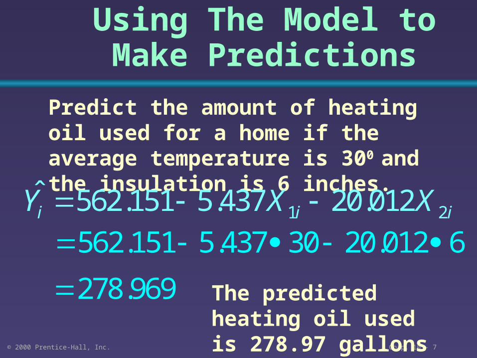
Using The Model to Make Predictions

Predict the amount of heating oil used for a home if the average temperature is 300 and the insulation is 6 inches.

The predicted heating oil used is 278.97 gallons

1 2ˆ 562.151 5.437 20.012i i iY X X

562.151 5.437 30 20.012 6

278.969


Developing the Model

Checking for problems.

Being sure the model passes all tests for model quality.


Identifying Problems

Do all the residual tests listed for simple regression.

Check for multicolinearity.


Multicolinearity

• This occurs when there is a high correlation between the explanatory variables.

• This leads to unstable coefficients .• The VIF used to measure colinearity

(values exceeding 5 are not good and exceeding 10 are a big problem):

,R

VIFj

j 21

1

2jR = Coefficient of Multiple

Determination of Xj

with all the others


Is the fit to the data good?


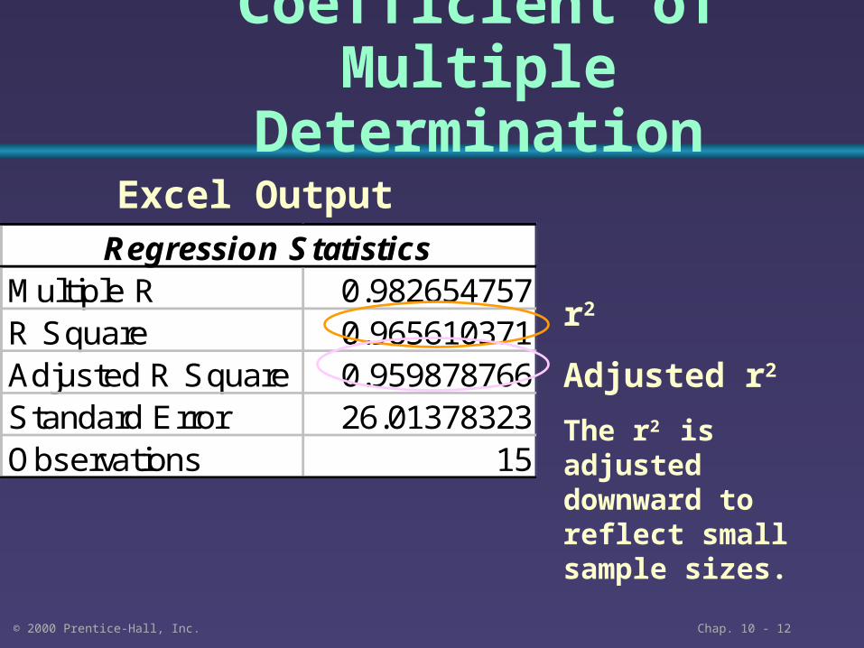
Coefficient of Multiple Determination

Regression StatisticsMultiple R 0.982654757R Square 0.965610371Adjusted R Square 0.959878766Standard Error 26.01378323Observations 15

Excel Output

r2

Adjusted r2

The r2 is adjusted downward to reflect small sample sizes.


Do the variables collectively pass the test?


Testing for Overall Significance

•Shows if there is a linear relationship between all of the X variables taken together and Y

•Hypothesis:

H0: 1 = 2 = … = p = 0 (No linear relationships)

H1: At least one i 0 (At least one independent variable effects Y)


ANOVAdf SS MS F Significance F

Regression 2 228014.6 114007.3 168.4712 1.65411E-09Residual 12 8120.603 676.7169Total 14 236135.2

Test for Overall SignificanceExcel Output: Example

p = 2, the number of explanatory variables n - 1

MSRMSE

p value

= F Test Statistic


F0 3.89

H0: 1 = 2 = … = p = 0

H1: At least one I 0 = .05

df = 2 and 12

Critical value(s):

Test Statistic:

Decision:

Conclusion:

Reject at = 0.05

There is evidence that at least one independentvariable affects Y.

= 0.05

F

Test for Overall Significance

168.47(Excel Output)


Test for Significance:Individual Variables

•Shows if there is a linear relationship between each

variable Xi and Y.

•Hypotheses:

H0: i = 0 (No linear relationship)

H1: i 0 (Linear relationship between Xi and Y)


Coefficients Standard Error t StatIntercept 562.151009 21.09310433 26.65094X Variable 1 -5.4365806 0.336216167 -16.1699X Variable 2 -20.012321 2.342505227 -8.54313

T Test StatisticExcel Output: Example

t Test Statistic for X1 (Temperature)

t Test Statistic for X2 (Insulation)

k

k

b

btS


H0: 1 = 0

h1: 1 0

df = n-2 = 12 critical value(s):

Test Statistic:

Decision:

Conclusion:

Reject H0 at = 0.05

There is evidence of a significant effect of temperature on oil

consumption.t0 2.1788-2.1788

.025

Reject H0 Reject H0

.025

Does temperature have a significant effect on monthly consumption of heating oil? Test at = 0.05.

t Test : Example Solution

t Test Statistic = -16.1699


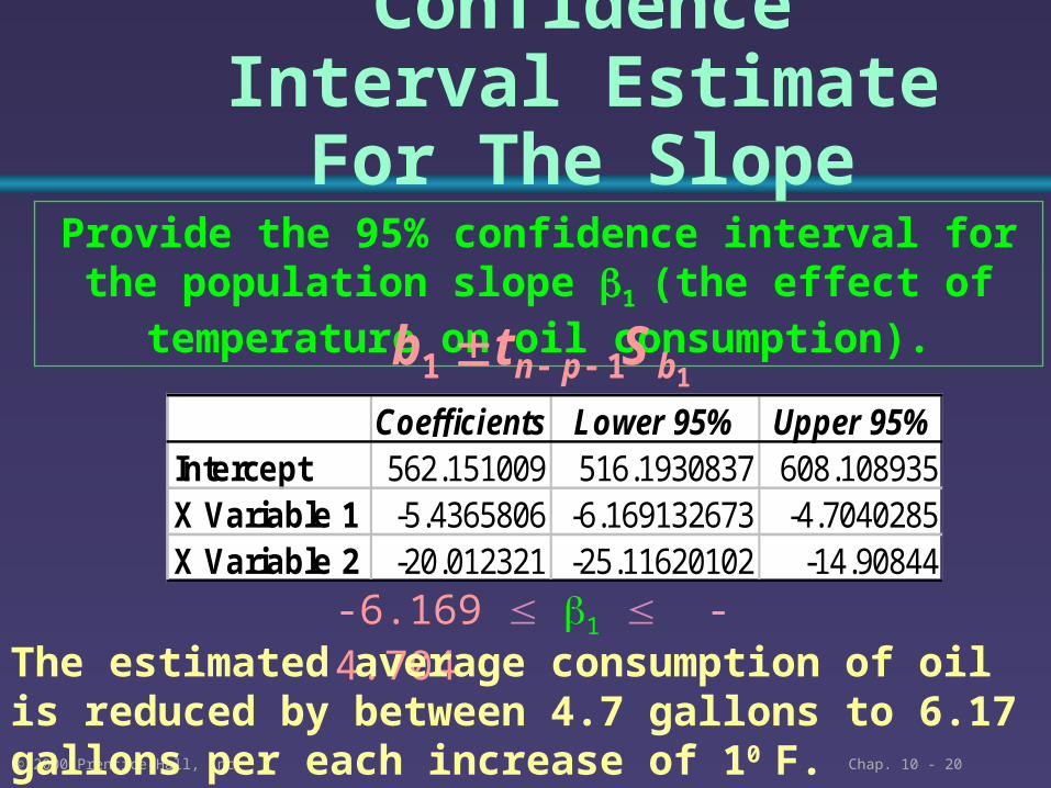
Confidence Interval Estimate For The Slope

Provide the 95% confidence interval for the population slope 1 (the effect of temperature on oil consumption).

111 bpn Stb Coefficients Lower 95% Upper 95%

Intercept 562.151009 516.1930837 608.108935X Variable 1 -5.4365806 -6.169132673 -4.7040285X Variable 2 -20.012321 -25.11620102 -14.90844

-6.169 1 -4.704The estimated average consumption of oil is reduced by between 4.7 gallons to 6.17 gallons per each increase of 10 F.


Special Regression Topics


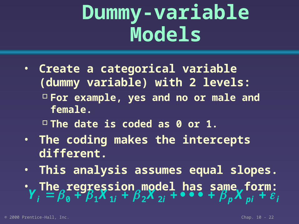
Dummy-variable Models

• Create a categorical variable (dummy variable) with 2 levels: For example, yes and no or male and female. The date is coded as 0 or 1.

• The coding makes the intercepts different.

• This analysis assumes equal slopes.

• The regression model has same form: ipipiii XXXY 22110


Dummy-variable Models Assumption

Given:

Y = Assessed Value of House

X1 = Square footage of House

X2 = Desirability of Neighborhood =

Desirable (X2 = 1)

Undesirable (X2 = 0)

iii Xb)bb()(bXbbY 11202110 1

0 if undesirable 1 if desirable

iii Xbb)(bXbbY 1102110 0

iii XbXbbY 22110

Same slopes


Dummy-variable Models Assumption

X1 (Square footage)

Y (Assessed Value)

Desirable Location

Undesirableb0 + b2

b0

Same slopes

Intercepts different


Interpretation of the Dummy Variable Coefficient

For example:

0 1 1 2 2i i iY b b X b X

1X

1 220 5 6i iX X

: GPA2X

0 Female

1 Male

Y: Annual salary of college graduate in thousand $

This 6 is interpreted as given the same GPA, the male college graduate is making an estimated 6 thousand dollars more than female on average.

:

© 2000 Prentice-Hall, Inc. Chap. 10 - 1 Multiple Regression Models.

Documents

Transcript of © 2000 Prentice-Hall, Inc. Chap. 10 - 1 Multiple Regression Models.