MARINE ECOLOGY PROGRESS SERIESMar Ecol Prog Ser

Vol. 663: 157–177, 2021https://doi.org/10.3354/meps13637

Published March 31

1. INTRODUCTION

There has been a call for unified approaches tostudying animal movement ecology (Nathan et al. 2008)

and using movement to understand ecosystem change(Hazen et al. 2019, Lowerre-Barbieri et al. 2019b) andim prove fisheries management (Link et al. 2020).Movement affects vulnerability to fishing and spatially

© Inter-Research 2021 · www.int-res.com*Corresponding author: elasmophile@gmail.com#These authors contributed equally to this work

Regional-scale variability in the movement ecologyof marine fishes revealed by an integrative acoustic

tracking network

Claudia Friess1,*,# , Susan K. Lowerre-Barbieri1,2,#, Gregg R. Poulakis3, Neil Hammerschlag4,Jayne M. Gardiner5, Andrea M. Kroetz6, Kim Bassos-Hull7, Joel Bickford1, Erin C. Bohaboy8,

Robert D. Ellis1, Hayden Menendez1, William F. Patterson III2, Melissa E. Price9, Jennifer S. Rehage10, Colin P. Shea1, Matthew J. Smukall11, Sarah Walters Burnsed1, Krystan A. Wilkinson7,12, Joy Young13, Angela B. Collins1,14, Breanna C. DeGroot15, Cheston T. Peterson16, Caleb Purtlebaugh17, Michael Randall9, Rachel M. Scharer3,

Ryan W. Schloesser7, Tonya R. Wiley18, Gina A. Alvarez19, Andy J. Danylchuk20, Adam G. Fox19, R. Dean Grubbs21, Ashley Hill22, James V. Locascio7, Patrick M. O’Donnell23,

Gregory B. Skomal24, Fred G. Whoriskey25, Lucas P. Griffin20

1Fish and Wildlife Research Institute, Florida Fish and Wildlife Conservation Commission, St. Petersburg, FL 33701, USA

Full author addresses are given in the Appendix

ABSTRACT: Marine fish movement plays a critical role in ecosystem functioning and is increas-ingly studied with acoustic telemetry. Traditionally, this research has focused on single speciesand small spatial scales. However, integrated tracking networks, such as the Integrated Trackingof Aquatic Animals in the Gulf of Mexico (iTAG) network, are building the capacity to monitormultiple species over larger spatial scales. We conducted a synthesis of passive acoustic monitor-ing data for 29 species (889 transmitters), ranging from large top predators to small consumers,monitored along the west coast of Florida, USA, over 3 yr (2016−2018). Space use was highly vari-able, with some groups using all monitored areas and others using only the area where they weretagged. The most extensive space use was found for Atlantic tarpon Megalops atlanticus and bullsharks Carcharhinus leucas. Individual detection patterns clustered into 4 groups, ranging from occa-sionally detected long-distance movers to frequently detected juvenile or adult residents. Synchro-nized, alongshore, long-distance movements were found for Atlantic tarpon, cobia Rachycentroncanadum, and several elasmobranch species. These movements were predominantly northboundin spring and southbound in fall. Detections of top predators were highest in summer, except fornearshore Tampa Bay where the most detections occurred in fall, coinciding with large red drumSciaenops ocellatus spawning aggregations. We discuss the future of collaborative telemetry re -search, including current limitations and potential solutions to maximize its impact for understand-ing movement ecology, conducting ecosystem monitoring, and supporting fisheries management.

KEY WORDS: Acoustic monitoring · Movement ecology · Ecosystem monitoring · IntegratedTracking of Aquatic Animals in the Gulf of Mexico · iTAG · Collaboration

Resale or republication not permitted without written consent of the publisher

Mar Ecol Prog Ser 663: 157–177, 2021

explicit stressors (Lowerre-Barbieri et al. 2019b), andvariation in migration, movement, or location can re-sult in perceived changes in marine populations of in-terest to managers (Link et al. 2020). In particular, abetter understanding of top predator spatiotemporalabundance and movement patterns is needed becausethey can serve as climate and ecosystem sentinels forwhich monitored attributes (including movement) in-dicate ecosystem change (Hays et al. 2016, Hazen etal. 2019). Additionally, habitat use by top predatorscan directly affect abundance and behavior of lowertrophic levels (Hammerschlag et al. 2012, Shoji et al.2017), an important consideration in fisheries manage-ment, as many top predator populations are underthreat from fisheries (Queiroz et al. 2019), while othersare showing signs of recovery from overfishing (Peter-son et al. 2017). A seasonal influx of predators to anarea could lead to seasonal predation mortality patternsand, if coinciding with a high-discard rate fishing sea-son, higher-than expected discard mortality levels.

Acoustic telemetry is a valuable tool for studyingmovement dynamics, migration, or centers of abun-dance of aquatic species (Abecasis et al. 2018) andhas been widely used in marine and freshwaterenvironments (Donaldson et al. 2014, Crossin et al.2017). Acoustic telemetry uses underwater hydro -phones (here after referred to as receivers), typicallyfixed in place and arranged in space and time withina specific ‘array’ of receivers according to researchobjectives (Brownscombe et al. 2019). Aquatic ani-mals outfitted with acoustic transmitters are detectedby receivers when they come within detection range,usually less than 500 m (Collins et al. 2008, Kessel etal. 2014b, Mathies et al. 2014). Research applicationsusing acoustic telemetry have included studying lifehistory aspects, such as timing and location of spawn-ing (Lowerre-Barbieri et al. 2016, Brownscombe et al.2020); assessing levels of discard mortality (Bohaboyet al. 2020); studying the effects of artificial reefs onsite fidelity and habitat connectivity (Keller et al.2017); examining the effects of ecotourism on behav-ior (Hammerschlag et al. 2017); monitoring compli-ance with no-fishing zones (Tickler et al. 2019); andevaluating the design of protected areas (Lea et al.2016, Griffin et al. 2020).

Acoustic tags can be detected on any receiver thatrecords within the frequencies transmitted by thetags. Given the mobility of many aquatic species andthe connectivity of aquatic systems, acoustic tags areoften opportunistically detected on outside receiverarrays (i.e. those deployed in other areas by re -searchers tracking a different set of animals). Tofacilitate the exchange of data between taggers and

acoustic array owners, several regional tracking net-works have formed, including the Australian Inte-grated Marine Observing System Animal TrackingFacility (IMOS ATF), Atlantic Cooperative Telemetry(ACT), Florida Atlantic Coast Telemetry (FACT; in -cluding arrays from the Carolinas to the Bahamas),and Integrated Tracking of Aquatic Animals in theGulf of Mexico (iTAG) networks. These networks ex -pand the geographic area over which tagged animalscan be tracked, thereby widening the scope of indi-vidual telemetry studies. Concurrently, conglomeratessuch as the Ocean Tracking Network (OTN) serve asdata repositories and facilitators for the various track-ing networks and telemetry studies. However, thereis a need to better leverage the strength of these net-works to address the challenges facing our ocean eco-systems (McGowan et al. 2017, Abecasis et al. 2018).A number of tools exist that facilitate such retrospec-tive analyses (Udyawer et al. 2018), but there are oftenlarge differences in array design and transmittersettings that cannot be fully accounted for duringstandardization for data analysis and limit the scopeof the questions that can be asked of these data.

The goal of this study was to evaluate how an inte-grative tracking approach can provide multi-speciesmovement data to improve our understanding ofmovement ecology and ecosystem processes, with aspecific focus on the seasonal movements of predatorsoff the west coast of Florida (WCF), USA. We analyzed3 years of data (2016−2018) from 21 acoustic telemetryarrays within the iTAG network in the eastern Gulf ofMexico (Gulf) to investigate the following 4 hypotheses:(1) array coverage needed to track a given speciesvaries based on movements and space use by thatspecies, (2) movements vary due to external factors,motion capacity, and navigation capacity (Nathan etal. 2008); thus species, tagging location, and life stageaffect observed movement patterns, (3) there is com-monality among species in seasonality and direction-ality of movement, indicating similar underlying bio-physical movement drivers, and (4) top predatordetection patterns show seasonal and spatial trends.Multiple analytical approaches were used to addressthese hypo theses, including quantification of detectionmetrics, clustering analysis, and predictive modeling.

2. MATERIALS AND METHODS

2.1. Study areas

Data from 21 acoustic receiver arrays belonging tothe iTAG regional tracking network in the eastern

158

Friess et al.: Multi-species movement dynamics 159

Gulf were used in this analysis (details about theindividual iTAG arrays can be found in Supplement 1and Table S1.1 at www. int-res. com/ articles/ suppl/m663 p157_ supp/). These iTAG arrays, deployed onthe WCF during the study period (2016−2018), allconsisted of Vemco receivers capable of detecting69 kHz acoustic transmitters. Their locations cov-ered the range of the entire WCF, but they werenot evenly distributed. Because iTAG arrays weredeveloped to address individual study-scale objec-tives, they exhibited a wide range of designs, vary-ing in receiver number (3−60) and distribution (e.g.gate, grid), with the finest spatial resolution comingfrom arrays set up as Vemco Positioning Systems(VPS).

It was necessary to regroup the receivers of someiTAG arrays to form spatially distinct units for an -alysis, resulting in 22 meta-arrays (referred to here-after as arrays) (Fig. 1; Table S2.1 in Supplement 2at www. int-res. com/ articles/ suppl/ m663 p157 _ supp/).These arrays were further aggregated into nodesfor some analyses to reduce the spatial bias createdby heterogeneity in array distribution (Fig. 1). In thepresent study, we referred to the arrays using the fol-

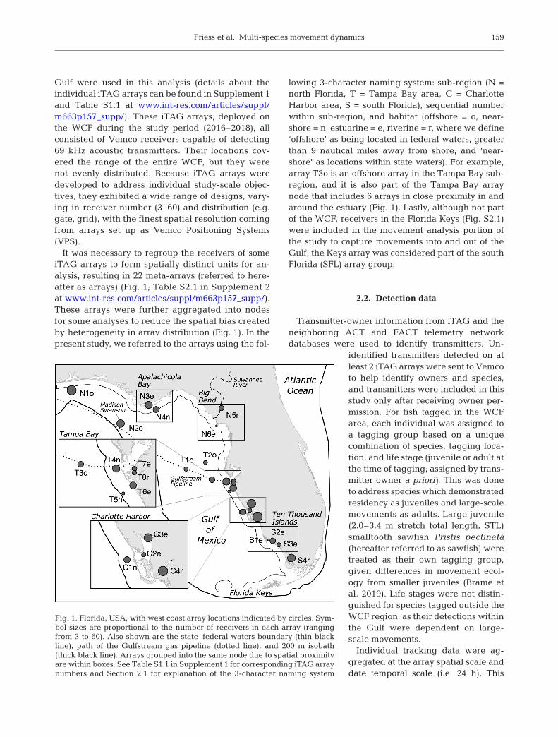
lowing 3-character naming system: sub-region (N =north Florida, T = Tampa Bay area, C = CharlotteHarbor area, S = south Florida), sequential numberwithin sub-region, and habitat (offshore = o, near-shore = n, estuarine = e, riverine = r, where we define‘offshore’ as being located in federal waters, greaterthan 9 nautical miles away from shore, and 'near-shore' as locations within state waters). For example,array T3o is an offshore array in the Tampa Bay sub-region, and it is also part of the Tampa Bay arraynode that includes 6 arrays in close proximity in andaround the estuary (Fig. 1). Lastly, although not partof the WCF, receivers in the Florida Keys (Fig. S2.1)were included in the movement analysis portion ofthe study to capture movements into and out of theGulf; the Keys array was considered part of the southFlorida (SFL) array group.

2.2. Detection data

Transmitter-owner information from iTAG and theneighboring ACT and FACT telemetry networkdatabases were used to identify transmitters. Un -

identified transmitters detected on atleast 2 iTAG arrays were sent to Vemcoto help identify owners and species,and transmitters were in cluded in thisstudy only after receiving owner per-mission. For fish tagged in the WCFarea, each individual was assigned toa tagging group based on a uniquecombination of species, tagging loca-tion, and life stage (juvenile or adult atthe time of tagging; assigned by trans-mitter owner a priori). This was doneto address species which demonstratedresidency as juveniles and large-scalemovements as adults. Large juvenile(2.0–3.4 m stretch total length, STL)smalltooth sawfish Pristis pectinata(hereafter referred to as sawfish) weretreated as their own tagging group,given differences in movement ecol-ogy from smaller juveniles (Brame etal. 2019). Life stages were not distin-guished for species tagged outside theWCF region, as their detections withinthe Gulf were dependent on large-scale movements.

Individual tracking data were ag -gregated at the array spatial scale anddate temporal scale (i.e. 24 h). This

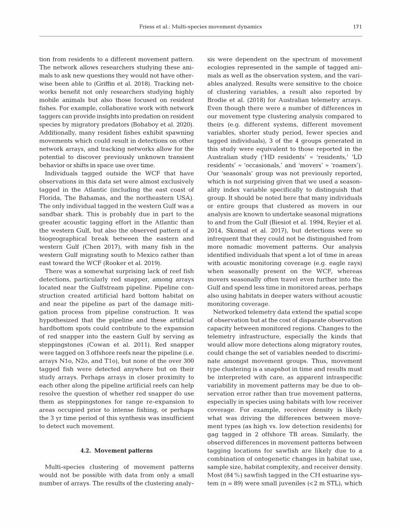
Fig. 1. Florida, USA, with west coast array locations indicated by circles. Sym-bol sizes are proportional to the number of receivers in each array (rangingfrom 3 to 60). Also shown are the state−federal waters boundary (thin blackline), path of the Gulfstream gas pipeline (dotted line), and 200 m isobath(thick black line). Arrays grouped into the same node due to spatial proximityare within boxes. See Table S1.1 in Supplement 1 for corresponding iTAG array numbers and Section 2.1 for explanation of the 3-character naming system

Mar Ecol Prog Ser 663: 157–177, 2021

allowed us to: (1) control for differences in studydesign (e.g. different transmitters and transmitterdelay programming; different array designs), (2) alignwith the scope of this study to assess movementacross the entire WCF rather than at small spatialscales, and (3) avoid overlap with ongoing and futureanalyses at the species-specific study scale. Animalswith a known fate of shed transmitters, or mortality(as evidenced by lack of vertical or lateral move-ment or change in movement signature) wereremoved prior to analysis, as were any animals withless than a 10 d detection period (defined as theperiod from tagging date or study start date, which -ever came first, until last detection date on the WCFor in the Florida Keys). Two detection filters, basedon R package ‘glatos’ functions (Binder et al. 2018),were used to remove potentially spurious detectionsbefore analysis: for a detection to be consideredvalid, there had to be at least 2 detections within anode in a 24 h period; or for VPS arrays, at least 2detections on a single receiver within a 24 h period.This stricter validation for VPS arrays was chosen toavoid including spurious detections which weremore likely to occur with overlapping receiverranges and large numbers of high site fidelity ani-mals tagged near receivers. Detection day (DD) wasdefined as a transmitter detected within an array ona calendar day. If a transmitter was detected at differ-ent arrays on the same day, multiple DDs wereassigned. DD data were summarized and visualizedusing the ‘tidyverse’ R package collection (Wickhamet al. 2019).

2.3. Movement patterns

We used clustering to analyze movement patterns.Clustering was done on individual-based movementvariables (see below) created from the networkedtelemetry data, which were first filtered for fish withpotential detection periods of at least 12 mo to evalu-ate the detection period for potential seasonal effects.Clustering was performed using the fuzzy C-meansclustering algorithm of Bezdek (1981) implementedin the R package ‘ppclust’ (Cebeci 2019). Two clustervalidity indices were used to determine optimumcluster size for a given set of variables: the fuzzy sil-houette index and the modified partition coefficientindex computed with the R package ‘fclust’ (Ferraroet al. 2019). The optimum number of clusters is thatfor which the index takes on the largest value. Clus-tering was done with different sets of exploratoryvariables thought to capture the detection pattern

variability among existing groups, and the finalmovement variables in the analysis were chosensuch that both cluster validity indices agreed on opti-mal cluster size (Table S2.2). The 4-cluster solutionprovided the clearest interpretability and was chosendue to the a priori ex pectation of 4 movement typesranging from highly resident to roaming or nomadic,similar to what has been described in the literature(Abrahms et al. 2017, Brodie et al. 2018). The result-ing clusters were as signed names a posteriori basedon movement variable distributions.

The 5 movement variables used in the analysiswere: 1 distance-related measure (the 99th quantileof distance traveled between successive detections),2 detection frequency variables (the residence indexand the 99th quantile of days between successiveDDs on the WCF), 1 seasonality indicator variable (aseasonality index), and 1 detection consistency index(the gap ratio defined as the 99th to 75th quantiles ofdays between successive DDs; see Table S2.3 forvariable summary statistics). Following Brodie et al.(2018), we used the 99th quantiles rather than 100th

quantiles to provide better metrics of the movementdata distribution. Residence index (RI) was the num-ber of days an individual was detected on the WCFdivided by the detection period. The seasonalityindex was calculated using time series decomposi-tion of the number of DDs mo−1 over the detectionperiod (see details in Supplement 2). The gap ratio islow for individuals lacking variation in temporaldetection patterns and high for those characterizedby periods of both increased and decreased numbersof DDs, regardless of whether or not these follow aseasonal trend. For each tagging group, the propor-tion of individuals in each movement group was cal-culated, and within-tagging group variability inmovement group was estimated by calculating thedeviation from the mode, which ranges from 0 (novariability) to 1 (equal proportions).

2.4. Movement pathways

Seasonality and directionality in observed move-ment pathways were examined for species exhibitinglong-distance movements to and from the FloridaKeys. Where species-specific data were insufficient,groupings of species with similar life history, move-ment ecology, and shared taxonomy were created.This resulted in a ‘coastal sharks’ group consisting ofgreat hammerhead Sphyrna mokarran, tiger Galeo-cerdo cuvier, lemon Negaprion brevirostris, andsandbar Carcharhinus plumbeus sharks. Movements

160

Friess et al.: Multi-species movement dynamics

were analyzed at the relatively coarse scale of calen-dar season (winter = December−February, spring =March−May, summer = June−August, fall = Septem-ber−November) and node. Even though movementswere not expected to coincide perfectly with calen-dar season, these time bins allowed for comparisonsof intra-annual patterns across species. Directed sea-sonal movement networks were created, and move-ments were classified according to alongshore direc-tionality (northbound or southbound). To ensure thevalidity of seasonal comparisons, 2 successive obser-vations were only counted as a movement if theyoccurred within a specific time period. This differedamong species and was based on visual inspection ofthe time between DD quantiles for each group (seedetails in Supplement 2 and Fig. S2.2). Resultingcut-off values ranged from 57 d for cobia to 80 d forAtlantic tarpon (hereafter referred to as tarpon). Sea-sonal movement networks were constructed andvisualized using the R packages ‘igraph’ (Csardi &Nepusz 2006), ‘ggplot2’ (Wickham et al. 2019), and‘ggraph’ (Pedersen 2020).

Generalized linear models (GLMs) were used todetect differences in the number of movement path-ways (i.e. network edges) observed by movementdirection and season. For each species group, modelswith and without an interaction between season andmovement direction were fitted. The response vari-able was edge weight, which was a count of the num-ber of times a potential movement path (between 2different nodes) was used. It was assumed to follow anegative binomial distribution. Since not all possiblemovement paths would be expected to be used by allspecies, a potential movement path was defined as apath that was observed to be traveled by that species,in either direction, during at least 1 season. Zerocounts were assigned to unused potential movementpaths. All models were fitted in the R package ‘rstan-arm’ (Goodrich et al. 2020) which uses Stan (Carpen-ter et al. 2017) for back-end estimation. Some combi-nations of season and movement path direction hadvery low or no positive observations, causing separa-tion in the data that led to estimation problems withstandard GLMs using maximum likelihood. Therefore,we chose Bayesian inference with weakly informa-tive priors which can help obtain stable regressioncoefficients and standard error estimates when sepa-ration is present in the data (Gelman et al. 2008). Allmodels used 4 Markov chains with 2000 iterationseach, discarding 1000 as ‘burn-in,’ and all priors werethe default priors provided by ‘rstanarm’ (weaklyinformative, normal priors with mean 0 and standarddeviation 2.5). We assessed convergence by calculat-

ing the potential scale reduction R̂ statistic (ensuringthat it was at most 1.1), inspecting trace plots, andensuring effective sample sizes of at least 1000 for allparameters. Model fit was assessed using leave-one-out cross-validation functionality provided by the Rpackage ‘loo’ (Vehtari et al. 2017), and the model withthe higher weight was used for inference. Model fitswere inspected graphically by conducting posteriorpredictive checks using the R packages ‘bayesplot’(Gabry & Mahr 2020) and ‘shinystan’ (Gabry 2018).

Marginal mean effects were computed and con-trasted using the R package ‘emmeans’ (Lenth 2019)to look for evidence of directional movement withinseason (pairwise contrast) and whether directionalmovements differed between seasons (i.e. comparingeach season to the average over all other seasons).Hypothesis testing was done in the R package‘bayestestR’ (Makowski et al. 2019a) by evaluatingevidence for existence and significance of effects.Effect existence was assessed with the probability ofdirection metric, the probability that a parameter isstrictly positive or negative, which is the Bayesianequivalent of the frequentist p-value (Makowski et al.2019b). Any probability of direction estimates above97.5% were treated as strong evidence for effectexistence. Effect significance was assessed by calcu-lating the portion of the full posterior density that fellwithin the region of practical equivalence (ROPE; therange of parameter values that is equivalent to 0).The ROPE range was set from −0.18 to +0.18, as isrecommended for parameters expressed in log oddsratios, and values less than 5% in ROPE were consid-ered significant (Makowski et al. 2019b). Overall, weconsidered an effect important if there was evidencefor both effect existence and significance. We reportobserved trends in the data, and all explicitly statedcomparisons constitute important effects.

2.5. Top predator hotspots

To test if top predator detections differed signifi-cantly by season or location, we fitted 2 GLMs forgreat hammerheads, bull Carcharhinus leucas, tiger,sandbar, lemon, and white Carcharodon carchariassharks (individuals tagged as juveniles on the WCFwere excluded to omit nursery habitat use from theanalysis). The first model aimed to address whethertotal top predator detection days varied by area(definition below) and season (DD model). The sec-ond model ad dressed whether the total number ofunique individuals detected varied by area and sea-son (nind model). For both models, we were particu-

161

Mar Ecol Prog Ser 663: 157–177, 2021

larly interested in the interaction effect betweenarea and season. Only a few arrays had sufficientdata to be included in this analysis and someneeded to be combined, resulting in 4 areas of com-parison for this analysis: nearshore Charlotte Harbor(the C1n array), the northern shelf (arrays N1o andN2o), nearshore Tampa Bay (arrays T4n and T5n),and offshore Tampa Bay (arrays T2o and T3o). Theresponse variable for the DD model was a dailycount of the number of individuals de tected by areafor each calendar day during the 3 yr study period.The re sponse variable for the nind model was acount of the number of unique individuals detectedmo−1. Both were assumed to follow a Poisson distri-bution. The predictors for both models were area,season, number of transmitters available for detec-tion, and study year (defined as December throughNovember so as to not split winter across multipleyears). Study year was included as a predictor toaccount for temporal changes in telemetry arrayconfiguration (most notably, the C1n array waslargely re moved in 2018) and ecological effects (mostnotably, the exceptionally strong and long-lastingred tide event that affected coastal Tampa Bay [TB]and Charlotte Harbor [CH] areas in 2018). Numberof available transmitters was included becausesome individuals were tagged after this studybegan (nstart = 24, nend = 54). The models includedinteractions between area and season as well asarea and study year, an offset for the number ofavailable transmitters, and, for the DD model, anested random effect for month within year toaccount for temporal autocorrelation patterns in thedata. Specifying available transmitters as an offsetvariable results in modeling the response variableas rates rather than counts (i.e. number of animalsdetected per available transmitter). The models canbe written as follows, where i represents calendarday for the DD model and month for the nind model:

yi ~Poisson(μi)

E(yi ) = μi (1)

log(μi) = Areai × Seasoni + Areai × StudyYeari + log(Tagsi)+ (1|Yeari/Monthi ) (DD model only)

Yeari ~N(0, σyear2 )

Month:Yeari ~N(0, σ2month:year)

where yi is number of individuals observed d−1 forthe DD model and number of unique individuals ob -served mo−1 for the nind model, μi is the expectedcount, and log(Tagsi) is the offset term for number ofavailable transmitters. Models were fitted in the R

package ‘glmmTMB’ (Brooks et al. 2017), which usesLaplace approximations to the likelihood via Tem-plate Model Builder (Kristensen et al. 2015). Tem-poral autocorrelation was checked visually using theR package ‘forecast’ (Hyndman & Khandakar 2008).Models were validated by simulating and testingresiduals from the fitted models using the R package‘DHARMa’ (Hartig 2019). Post-hoc analyses wereconducted using the R package ‘emmeans,’ wheremarginal ef fects for the variables of interest (i.e. areaand season) were calculated and contrasted to testfor significance of season and study year effectswithin and among areas.

3. RESULTS

Detection data represented 889 fish from 29 species(Table 1). These species range in terms of manage-ment concerns from threatened and endangeredspecies (Gulf sturgeon Acipenser oxyrinchus desotoiand sawfish, respectively) to unmanaged species(e.g. hardhead Ariopsis felis and gafftopsail Bagremarinus catfish). Habitat use was similarly wide-ranging, from freshwater to offshore, with correspon-ding management responsibility divided betweenstate and federal agencies. The following list typifiesthe range from freshwater to marine life cycles: thefreshwater largemouth bass Micropterus salmoides,the diadromous common snook Centropomus undec-imalis (hereafter referred to as snook), the primarilyestuarine southern kingfish Menticirrhus ameri-canus, estuarine-dependent species (e.g. tarpon andred drum), reef fishes and elasmobranchs with estu-arine nurseries (e.g. gray snapper Lutjanus griseusand blacktip shark Carcharhinus limbatus), to off-shore species such as red snapper L. campechanusand white shark. The mean number of tagged fishspecies−1 was 31 but ranged from 1 (3 species) to 163individuals for sawfish (Table 1). Tagging dates var-ied over the study period, contributing to a range ofdetection periods from 1 to 899 d, with a relativelyshort mean detection period for all species (235 d).

The tracking network on the WCF varies in broadspatial acoustic monitoring coverage, array size (i.e.number of receivers), and habitat being monitored:riverine (n = 4), estuarine (n = 9), nearshore (n = 4),and offshore (n = 5) arrays (Fig. 1). Only 15% of theindividuals were observed in more than 1 node, butthese fish represented a fairly wide range of species:great hammerhead, blacktip, bull, lemon, sandbar,tiger, and white sharks, tarpon, cobia, snook, goliathgrouper Epinephelus itajara, greater amberjack Seri-

162

Friess et al.: Multi-species movement dynamics

ola dumerili, Gulf sturgeon, red drum, sawfish, andwhitespotted eagle ray Aetobatus narinari (hereafterreferred to as eagle ray).

3.1. Large-scale space use

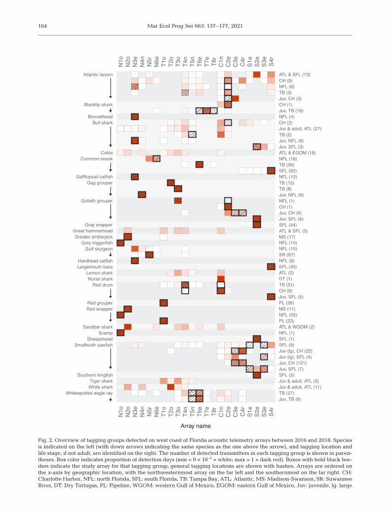
We detected 55 unique tagging groups on theWCF (Fig. 2). Species with multiple tagging groupsincluded tarpon, bull shark, gag grouper Myctero -perca microlepis, goliath grouper, Gulf sturgeon, reddrum, red snapper, sawfish, snook, blacktip shark,and eagle ray. Many tagging groups (49%) repre-sented fish tagged within the WCF and detected onmultiple arrays. Another 31% of the tagging groupswere detected only in their study arrays, a patterndriven by both site fidelity and proximity of a studyarray to other arrays. These species included mostreef fishes, the catfishes, southern kingfish, sheeps -head Archosargus probatocephalus, largemouth bass,and bonnethead Sphyrna tiburo (Fig. 2). Lastly, 18%of tagging groups were tagged outside the WCFregion, highlighting the role integrative tracking net-

works play for these species, which included a nurseshark Ginglymostoma cirratum as well as a numberof top predators (great hammerhead, bull, lemon,sandbar, tiger, and white sharks), which prey on manyof the resident species. The most expansive spaceuse on the WCF was seen for adult tarpon tagginggroups and bull sharks tagged in the Atlantic or CHarea (Fig. 2).

3.2. Movement patterns

The 4 groups generated by clustering of movementvariables for 554 individuals were characterized aposteriori as: long-distance movers that were detectedinfrequently (‘movers;’ n = 84), high-detection resi-dents (‘HD residents;’ n = 191), low-detection residents(‘LD residents;’ n = 168), and ‘seasonals’ (n = 111).Both resident groups traveled short maximal dis-tances between DDs (LD residents: mean ± SE = 7.4± 1.45 km; HD residents: 0.45 ± 0.36 km), but theydiffered in temporal detection patterns (Fig. 3). HDresidents (represented best by red snapper, red

163

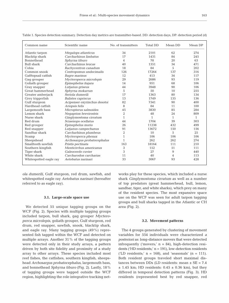
Common name Scientific name No. of transmitters Total DD Mean DD Mean DP

Atlantic tarpon Megalops atlanticus 34 2101 62 274Blacktip shark Carcharhinus limbatus 17 1431 84 245Bonnethead Sphyrna tiburo 4 78 20 63Bull shark Carcharhinus leucas 40 1351 34 471Cobia Rachycentron canadum 18 84 5 202Common snook Centropomus undecimalis 126 17264 137 316Gafftopsail catfish Bagre marinus 12 413 34 117Gag grouper Mycteroperca microlepis 29 2686 93 119Goliath grouper Epinephelus itajara 14 951 68 106Gray snapper Lutjanus griseus 44 3948 90 106Great hammerhead Sphyrna mokarran 5 50 10 255Greater amberjack Seriola dumerili 17 1363 80 134Grey triggerfish Balistes capriscus 13 1749 135 136Gulf sturgeon Acipenser oxyrinchus desotoi 82 7341 90 400Hardhead catfish Ariopsis felis 8 84 11 100Largemouth bass Micropterus salmoides 45 3830 85 284Lemon shark Negaprion brevirostris 2 48 24 809Nurse shark Ginglymostoma cirratum 1 1 1 1Red drum Sciaenops ocellatus 44 1704 39 303Red grouper Epinephelus morio 26 11238 432 499Red snapper Lutjanus campechanus 91 13672 150 156Sandbar shark Carcharhinus plumbeus 2 10 5 25Scamp Mycteroperca phenax 1 106 106 106Sheepshead Archosargus probatocephalus 1 262 262 274Smalltooth sawfish Pristis pectinata 163 18164 111 210Southern kingfish Menticirrhus americanus 3 152 51 111Tiger shark Galeocerdo cuvier 3 27 9 440White shark Carcharodon carcharias 11 40 4 113Whitespotted eagle ray Aetobatus narinari 33 3067 93 428

Table 1. Species detection summary. Detection day metrics are transmitter-based. DD: detection days, DP: detection period (d)

Mar Ecol Prog Ser 663: 157–177, 2021164

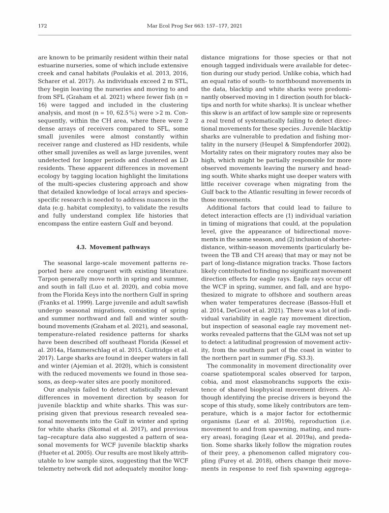
Fig. 2. Overview of tagging groups detected on west coast of Florida acoustic telemetry arrays between 2016 and 2018. Speciesis indicated on the left (with down arrows indicating the same species as the one above the arrow), and tagging location andlife stage, if not adult, are identified on the right. The number of detected transmitters in each tagging group is shown in paren-theses. Box color indicates proportion of detection days (min = 9 × 10−5 = white; max = 1 = dark red). Boxes with bold black bor-ders indicate the study array for that tagging group; general tagging locations are shown with hashes. Arrays are ordered onthe x-axis by geographic location, with the northwesternmost array on the far left and the southernmost on the far right. CH:Charlotte Harbor, NFL: north Florida, SFL: south Florida, TB: Tampa Bay, ATL: Atlantic, MS: Madison-Swanson, SR: SuwanneeRiver, DT: Dry Tortugas, PL: Pipeline, WGOM: western Gulf of Mexico, EGOM: eastern Gulf of Mexico, Juv: juvenile, lg: large

Friess et al.: Multi-species movement dynamics

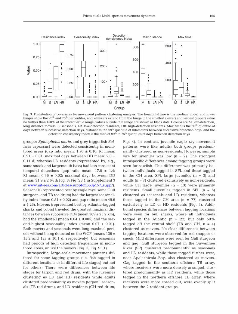
grouper Epinephelus morio, and grey triggerfish Bal-istes capriscus) were detected consistently in moni-tored areas (gap ratio mean: 1.93 ± 0.10; RI mean:0.91 ± 0.01; maximal days between DD mean: 2.0 ±0.11 d) whereas LD residents (represented by, e.g.,some snook and largemouth bass) had less consistenttemporal detections (gap ratio mean: 17.0 ± 1.4;RI mean: 0.36 ± 0.02; maximal days between DDmean: 31.9 ± 2.64 d; Fig. 3; Fig. S3.1 in Supplement 3at www. int-res. com/ articles/ suppl/ m663 p157 _ supp/).Seasonals (represented best by eagle rays, some Gulfsturgeon, and TB red drum) had the largest seasonal-ity index (mean 0.51 ± 0.02) and gap ratio (mean 49.6± 4.26). Movers (represented best by Atlantic-taggedsharks and cobia) traveled the greatest maximal dis-tances between successive DDs (mean 369 ± 25.2 km),had the smallest RI (mean 0.04 ± 0.005) and the sec-ond-highest seasonality index (mean 0.07 ± 0.01).Both movers and seasonals went long maximal peri-ods without being detected on the WCF (means 136 ±15.2 and 123 ± 10.1 d, respectively), but seasonalshad periods of high detection frequencies in moni-tored areas, unlike the movers (Fig. 3; Fig. S3.1).

Intraspecific, large-scale movement patterns dif-fered for some tagging groups (i.e. fish tagged indifferent locations or in different life stages) but notfor others. There were differences between lifestages for tarpon and red drum, with the juvenilesclustering as LD and HD residents while adultsclustered predominantly as movers (tarpon), season-als (TB red drum), and LD residents (CH red drum;

Fig. 4). In contrast, juvenile eagle ray movementpatterns were like adults; both groups predomi-nantly clustered as non-residents. However, samplesize for juveniles was low (n = 2). The strongestintraspecific differences among tagging groups wereseen for sawfish. This difference was primarily be -tween individuals tagged in SFL and those taggedin the CH area. SFL large juveniles (n = 3) andadults (n = 7) clustered exclusively as non-residents,while CH large juveniles (n = 13) were primarilyresidents. Small juveniles tagged in SFL (n = 6)clustered as seasonals and LD residents, whereasthose tagged in the CH area (n = 77) clusteredexclusively as LD or HD residents (Fig. 4). Addi-tional species differences between tagging locationswere seen for bull sharks, where all individualstagged in the Atlantic (n = 22) but only 50%tagged off the central shelf (TB and CH, n = 4)clustered as movers. No clear differences betweentagging locations were observed for red snapper orsnook. Mild differences were seen for Gulf sturgeonand gag. Gulf sturgeon tagged in the SuwanneeRiver (SR) clustered predominantly as seasonalsand LD residents, while those tagged further west,near Apalachicola Bay, also clustered as movers.Gag tagged in the southern offshore TB array,where re ceivers were more densely arranged, clus-tered predominantly as HD residents, while thosetagged in the northern offshore TB array, wherereceivers were more spread out, were evenly splitbetween the 2 resident groups.

165

Residence index Seasonality index Detection consistency index Max distance Max time

M LR HR M LR HR M LR HR M LR HR M LR HR

0

200

400

600

0

200

400

600

800

0

100

200

300

0.00

0.25

0.50

0.75

0.00

0.25

0.50

0.75

1.00

Group

Valu

e

SSSSS

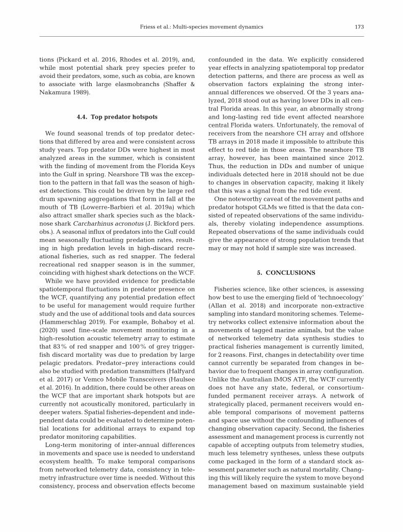
Fig. 3. Distribution of covariates for movement pattern clustering analysis. The horizontal line is the median, upper and lowerhinges show the 25th and 75th percentiles, and whiskers extend from the hinge to the smallest (lower) and largest (upper) valueno further than 150% of the interquartile range; values outside that range are shown as black dots. Groups are M: low-detection,long distance movers, S: seasonals, LR: low-detection residents, HR: high-detection residents. Max time is the 99th quantile ofdays between successive detection days, distance is the 99th quantile of kilometers between successive detection days, and the

detection consistency index is the ratio of 99th to 75th quantiles of days between detection days

Mar Ecol Prog Ser 663: 157–177, 2021

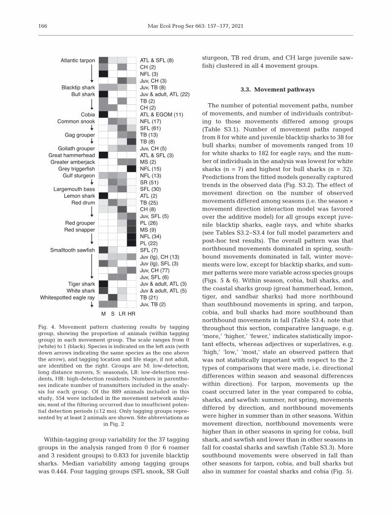
Within-tagging group variability for the 37 tagginggroups in the analysis ranged from 0 (for 6 roamerand 3 resident groups) to 0.833 for juvenile blacktipsharks. Median variability among tagging groupswas 0.444. Four tagging groups (SFL snook, SR Gulf

sturgeon, TB red drum, and CH large juvenile saw-fish) clustered in all 4 movement groups.

3.3. Movement pathways

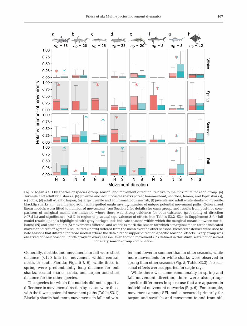
The number of potential movement paths, numberof movements, and number of individuals contribut-ing to those movements differed among groups(Table S3.1). Number of movement paths rangedfrom 8 for white and juvenile blacktip sharks to 38 forbull sharks; number of movements ranged from 10for white sharks to 182 for eagle rays; and the num-ber of individuals in the analysis was lowest for whitesharks (n = 7) and highest for bull sharks (n = 32).Predictions from the fitted models generally capturedtrends in the observed data (Fig. S3.2). The effect ofmovement direction on the number of observedmovements differed among seasons (i.e. the season ×movement direction interaction model was favoredover the additive model) for all groups except juve-nile blacktip sharks, eagle rays, and white sharks(see Tables S3.2−S3.4 for full model parameters andpost-hoc test results). The overall pattern was thatnorthbound movements dominated in spring, south-bound movements dominated in fall, winter move-ments were low, except for blacktip sharks, and sum-mer patterns were more variable across species groups(Figs. 5 & 6). Within season, cobia, bull sharks, andthe coastal sharks group (great hammerhead, lemon,tiger, and sandbar sharks) had more northboundthan southbound movements in spring, and tarpon,cobia, and bull sharks had more southbound thannorthbound movements in fall (Table S3.4; note thatthroughout this section, comparative language, e.g.‘more,’ ‘higher,’ ‘fewer,’ indicates statistically impor-tant effects, whereas adjectives or superlatives, e.g.‘high,’ ‘low,’ ‘most,’ state an observed pattern thatwas not statistically important with respect to the 2types of comparisons that were made, i.e. directionaldifferences within season and seasonal differenceswithin direction). For tarpon, movements up thecoast occurred later in the year compared to cobia,sharks, and sawfish: summer, not spring, movementsdiffered by direction, and northbound movementswere higher in summer than in other seasons. Withinmovement direction, northbound movements werehigher than in other seasons in spring for cobia, bullshark, and sawfish and lower than in other seasons infall for coastal sharks and sawfish (Table S3.3). Moresouthbound movements were observed in fall thanother seasons for tarpon, cobia, and bull sharks butalso in summer for coastal sharks and cobia (Fig. 5).

166

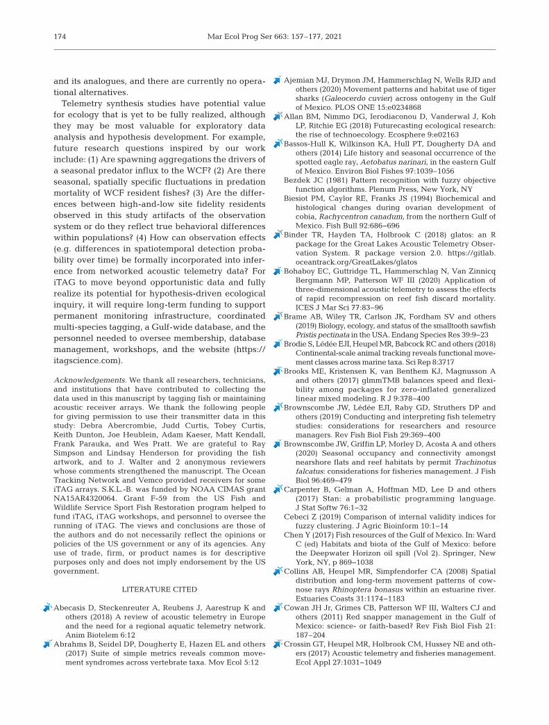
Fig. 4. Movement pattern clustering results by tagginggroup, showing the proportion of animals (within tagginggroup) in each movement group. The scale ranges from 0(white) to 1 (black). Species is indicated on the left axis (withdown arrows indicating the same species as the one abovethe arrow), and tagging location and life stage, if not adult,are identified on the right. Groups are M: low-detection,long distance movers, S: seasonals, LR: low-detection resi-dents, HR: high-detection residents. Numbers in parenthe-ses indicate number of transmitters included in the analy-sis for each group. Of the 889 animals included in thisstudy, 554 were included in the movement network analy-sis; most of the filtering occurred due to insufficient poten-tial detection periods (≤12 mo). Only tagging groups repre-sented by at least 2 animals are shown. Site abbreviations as

in Fig. 2

Friess et al.: Multi-species movement dynamics 167

Generally, northbound movements in fall were shortdistance (<120 km; i.e. movement within central,north, or south Florida; Figs. 5 & 6), while those inspring were predominantly long distance for bullsharks, coastal sharks, cobia, and tarpon and shortdistance for the other species.

The species for which the models did not support adifference in movement direction by season were thosewith the fewest potential movement paths (Table S3.1).Blacktip sharks had more movements in fall and win-

ter, and fewer in summer than in other seasons, whilemore movements for white sharks were observed inspring than other seasons (Fig. 5; Table S3.3). No sea-sonal effects were supported for eagle rays.

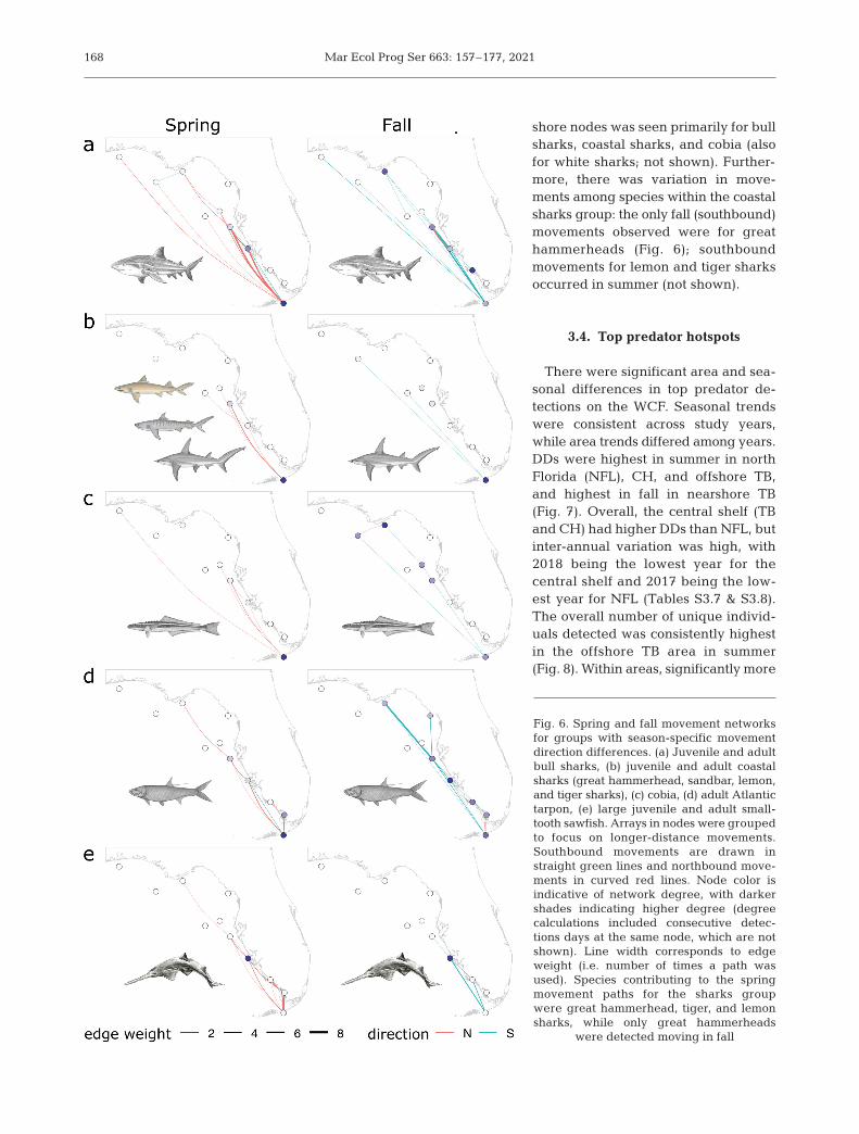
While there was some commonality in spring andfall movement direction, there were also group-specific differences in space use that are apparent inindividual movement networks (Fig. 6). For example,movement among SFL nodes occurred primarily fortarpon and sawfish, and movement to and from off-

Fig. 5. Mean + SD by species or species group, season, and movement direction, relative to the maximum for each group. (a)Juvenile and adult bull sharks, (b) juvenile and adult coastal sharks (great hammerhead, sandbar, lemon, and tiger sharks),(c) cobia, (d) adult Atlantic tarpon, (e) large juvenile and adult smalltooth sawfish, (f) juvenile and adult white sharks, (g) juvenileblacktip sharks, (h) juvenile and adult whitespotted eagle rays. np: number of unique potential movement paths. Generalizedlinear models were fitted to number of movements (see Section 2 for details) for each group, and results from post-hoc com-parisons of marginal means are indicated where there was strong evidence for both existence (probability of direction>97.5%) and significance (<5% in region of practical equivalence) of effects (see Tables S3.2−S3.4 in Supplement 3 for fullmodel results): panels highlighted with grey backgrounds indicate seasons within which the marginal means between north-bound (N) and southbound (S) movements differed, and asterisks mark the season for which a marginal mean for the indicatedmovement direction (green = south, red = north) differed from the mean over the other seasons. Bicolored asterisks were used tonote seasons that differed for those models where the data did not support direction-specific seasonal effects. Every group wasobserved on west coast of Florida arrays in every season, even though movements, as defined in this study, were not observed

for every season−group combination

Mar Ecol Prog Ser 663: 157–177, 2021

shore nodes was seen primarily for bullsharks, coastal sharks, and cobia (alsofor white sharks; not shown). Further-more, there was variation in move-ments among species within the coastalsharks group: the only fall (southbound)movements ob served were for greathammerheads (Fig. 6); southboundmovements for lemon and tiger sharksoccurred in summer (not shown).

3.4. Top predator hotspots

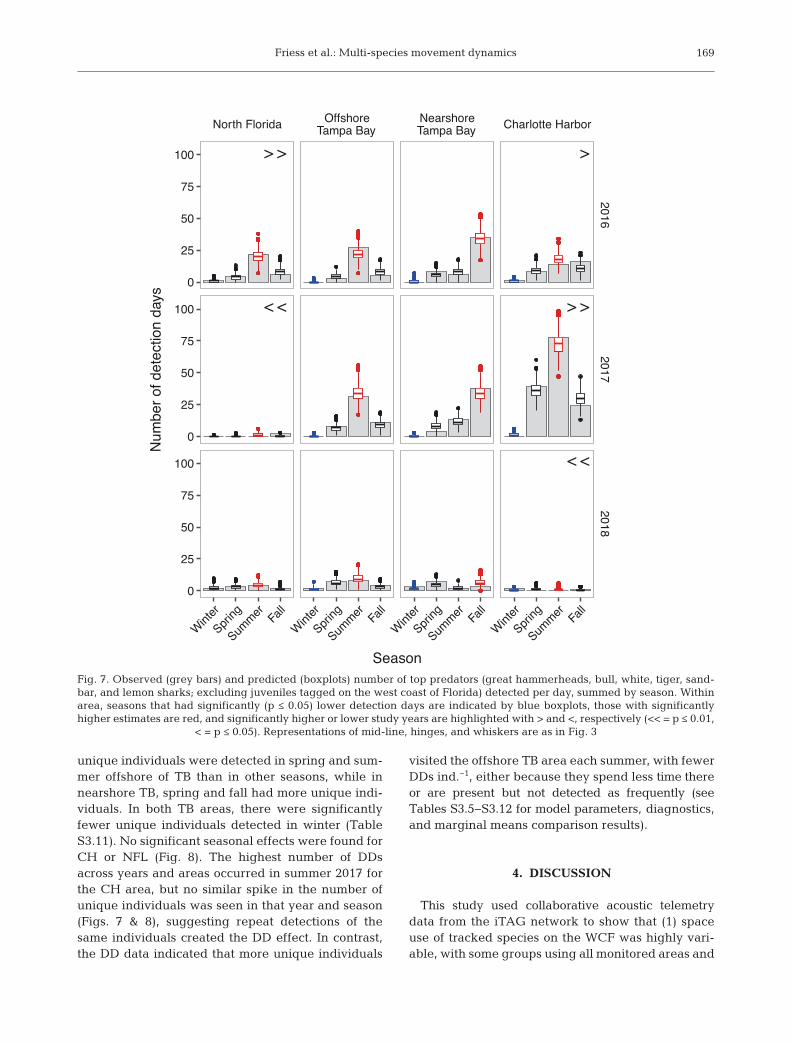
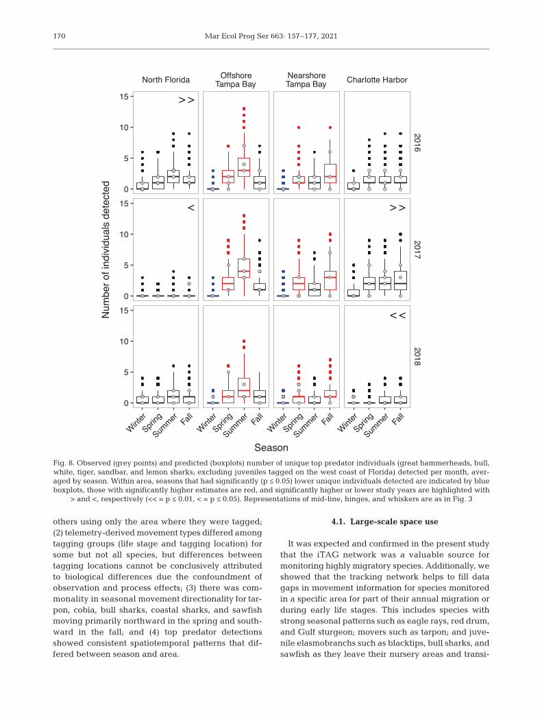
There were significant area and sea-sonal differences in top predator de -tections on the WCF. Seasonal trendswere consistent across study years,while area trends differed among years.DDs were highest in summer in northFlorida (NFL), CH, and offshore TB,and highest in fall in nearshore TB(Fig. 7). Overall, the central shelf (TBand CH) had higher DDs than NFL, butinter-annual variation was high, with2018 being the lowest year for thecentral shelf and 2017 being the low-est year for NFL (Tables S3.7 & S3.8).The overall number of unique individ-uals detected was consistently highestin the offshore TB area in summer(Fig. 8). Within areas, significantly more

168

Fig. 6. Spring and fall movement networksfor groups with season-specific movementdirection differences. (a) Juvenile and adultbull sharks, (b) juvenile and adult coastalsharks (great hammerhead, sandbar, lemon,and tiger sharks), (c) cobia, (d) adult Atlantictarpon, (e) large juvenile and adult small-tooth sawfish. Arrays in nodes were groupedto focus on longer-distance movements.South bound movements are drawn instraight green lines and northbound move-ments in curved red lines. Node color isindicative of network degree, with darkershades indicating higher degree (degreecalculations in cluded consecutive detec-tions days at the same node, which are notshown). Line width corresponds to edgeweight (i.e. number of times a path wasused). Species contributing to the springmovement paths for the sharks groupwere great hammerhead, tiger, and lemonsharks, while only great hammerheads

were detected moving in fall

Friess et al.: Multi-species movement dynamics

unique individuals were detected in spring and sum-mer offshore of TB than in other seasons, while innearshore TB, spring and fall had more unique indi-viduals. In both TB areas, there were significantlyfewer unique individuals detected in winter (TableS3.11). No significant seasonal effects were found forCH or NFL (Fig. 8). The highest number of DDsacross years and areas occurred in summer 2017 forthe CH area, but no similar spike in the number ofunique individuals was seen in that year and season(Figs. 7 & 8), suggesting repeat detections of thesame individuals created the DD effect. In contrast,the DD data indicated that more unique individuals

visited the offshore TB area each summer, with fewerDDs ind.−1, either because they spend less time thereor are present but not detected as frequently (seeTables S3.5−S3.12 for model parameters, diagnostics,and marginal means comparison results).

4. DISCUSSION

This study used collaborative acoustic telemetrydata from the iTAG network to show that (1) spaceuse of tracked species on the WCF was highly vari-able, with some groups using all monitored areas and

169

Fig. 7. Observed (grey bars) and predicted (boxplots) number of top predators (great hammerheads, bull, white, tiger, sand-bar, and lemon sharks; excluding juveniles tagged on the west coast of Florida) detected per day, summed by season. Withinarea, seasons that had significantly (p ≤ 0.05) lower detection days are indicated by blue boxplots, those with significantlyhigher estimates are red, and significantly higher or lower study years are highlighted with > and <, respectively (<< = p ≤ 0.01,

< = p ≤ 0.05). Representations of mid-line, hinges, and whiskers are as in Fig. 3

Mar Ecol Prog Ser 663: 157–177, 2021

others using only the area where they were tagged;(2) telemetry-derived movement types differed amongtagging groups (life stage and tagging location) forsome but not all species, but differences betweentagging locations cannot be conclusively attributedto biological differences due the confoundment ofobservation and process effects; (3) there was com-monality in seasonal movement directionality for tar-pon, cobia, bull sharks, coastal sharks, and sawfishmoving primarily northward in the spring and south-ward in the fall; and (4) top predator detectionsshowed consistent spatiotemporal patterns that dif-fered between season and area.

4.1. Large-scale space use

It was expected and confirmed in the present studythat the iTAG network was a valuable source formonitoring highly migratory species. Additionally, weshowed that the tracking network helps to fill datagaps in movement information for species monitoredin a specific area for part of their annual migration orduring early life stages. This includes species withstrong seasonal patterns such as eagle rays, red drum,and Gulf sturgeon; movers such as tarpon; and juve-nile elasmobranchs such as blacktips, bull sharks, andsawfish as they leave their nursery areas and transi-

170

Fig. 8. Observed (grey points) and predicted (boxplots) number of unique top predator individuals (great hammerheads, bull,white, tiger, sandbar, and lemon sharks; excluding juveniles tagged on the west coast of Florida) detected per month, aver-aged by season. Within area, seasons that had significantly (p ≤ 0.05) lower unique individuals detected are indicated by blueboxplots, those with significantly higher estimates are red, and significantly higher or lower study years are highlighted with

> and <, respectively (<< = p ≤ 0.01, < = p ≤ 0.05). Representations of mid-line, hinges, and whiskers are as in Fig. 3

Friess et al.: Multi-species movement dynamics

tion from residents to a different movement pattern.The network allows re searchers studying these ani-mals to ask new questions they would not have other-wise been able to (Griffin et al. 2018). Tracking net-works benefit not only researchers studying highlymobile animals but also those focused on residentfishes. For example, collaborative work with networktaggers can provide insights into predation on residentspecies by migratory predators (Bohaboy et al. 2020).Additionally, many resident fishes exhibit spawningmovements which could result in detections on othernetwork arrays, and tracking networks allow for thepotential to discover previously unknown transientbehavior or shifts in space use over time.

Individuals tagged outside the WCF that haveobservations in this data set were almost exclusivelytagged in the Atlantic (including the east coast ofFlorida, The Bahamas, and the northeastern USA).The only individual tagged in the western Gulf was asandbar shark. This is probably due in part to thegreater acoustic tagging effort in the Atlantic thanthe western Gulf, but also the observed pattern of abiogeographical break between the eastern andwestern Gulf (Chen 2017), with many fish in thewestern Gulf migrating south to Mexico rather thaneast toward the WCF (Rooker et al. 2019).

There was a somewhat surprising lack of reef fishdetections, particularly red snapper, among arrayslocated near the Gulfstream pipeline. Pipeline con-struction created artificial hard bottom habitat onand near the pipeline as part of the damage miti -gation process from pipeline construction. It washypothesized that the pipeline and these artificialhardbottom spots could contribute to the expansionof red snapper into the eastern Gulf by serving assteppingstones (Cowan et al. 2011). Red snapperwere tagged on 3 offshore reefs near the pipeline (i.e.arrays N1o, N2o, and T1o), but none of the over 300tagged fish were detected anywhere but on theirstudy arrays. Perhaps arrays in closer proximity toeach other along the pipeline artificial reefs can helpresolve the question of whether red snapper do usethem as steppingstones for range re-expansion toareas occupied prior to intense fishing, or perhapsthe 3 yr time period of this synthesis was insufficientto detect such movement.

4.2. Movement patterns

Multi-species clustering of movement patternswould not be possible with data from only a smallnumber of arrays. The results of the clustering analy-

sis were dependent on the spectrum of movementecologies represented in the sample of tagged ani-mals as well as the observation system, and the vari-ables analyzed. Results were sensitive to the choiceof clustering variables, a result also reported byBrodie et al. (2018) for Australian telemetry arrays.Even though there were a number of differences inour movement type clustering analysis compared totheirs (e.g. different systems, different movementvariables, shorter study period, fewer species andtagged individuals), 3 of the 4 groups generated inthis study were equivalent to those reported in theAustralian study (‘HD residents’ ≈ ‘residents,’ ‘LDresidents’ ≈ ‘occasionals,’ and ‘movers’ ≈ ‘roamers’).Our ‘seasonals’ group was not previously reported,which is not surprising given that we used a season-ality index variable specifically to distinguish thatgroup. It should be noted here that many individualsor entire groups that clustered as movers in ouranalysis are known to undertake seasonal migrationsto and from the Gulf (Biesiot et al. 1994, Reyier et al.2014, Skomal et al. 2017), but detections were soinfrequent that they could not be distinguished frommore nomadic movement patterns. Our analysisidentified individuals that spent a lot of time in areaswith acoustic monitoring coverage (e.g. eagle rays)when seasonally present on the WCF, whereasmovers seasonally often travel even further into theGulf and spend less time in monitored areas, perhapsalso using habitats in deeper waters without acousticmonitoring coverage.

Networked telemetry data extend the spatial scopeof observation but at the cost of disparate observationcapacity between monitored regions. Changes to thetelemetry infrastructure, especially the kinds thatwould allow more detections along migratory routes,could change the set of variables needed to discrimi-nate amongst movement groups. Thus, movementtype clustering is a snapshot in time and results mustbe interpreted with care, as apparent intraspecificvariability in movement patterns may be due to ob -servation error rather than true movement patterns,especially in species using habitats with low receivercoverage. For example, receiver density is likelywhat was driving the differences between move-ment types (as high vs. low detection residents) forgag tagged in 2 offshore TB areas. Similarly, theobserved differences in movement patterns betweentagging locations for sawfish are likely due to acombination of ontogenetic changes in habitat use,sample size, habitat complexity, and receiver density.Most (84%) sawfish tagged in the CH estuarine sys-tem (n = 89) were small juveniles (<2 m STL), which

171

Mar Ecol Prog Ser 663: 157–177, 2021

are known to be primarily resident within their natalestuarine nurseries, some of which include extensivecreek and canal habitats (Poulakis et al. 2013, 2016,Scharer et al. 2017). As individuals exceed 2 m STL,they begin leaving the nurseries and moving to andfrom SFL (Graham et al. 2021) where fewer fish (n =16) were tagged and included in the clusteringanalysis, and most (n = 10, 62.5%) were >2 m. Con-sequently, within the CH area, where there were 2dense arrays of receivers compared to SFL, somesmall juveniles were almost constantly withinreceiver range and clustered as HD residents, whileother small juveniles as well as large juveniles, wentundetected for longer periods and clustered as LDresidents. These apparent differences in movementecology by tagging location highlight the limitationsof the multi-species clustering approach and showthat detailed knowledge of local arrays and species-specific re search is needed to address nuances in thedata (e.g. habitat complexity), to validate the resultsand fully understand complex life histories thatencompass the entire eastern Gulf and beyond.

4.3. Movement pathways

The seasonal large-scale movement patterns re -ported here are congruent with existing literature.Tarpon generally move north in spring and summer,and south in fall (Luo et al. 2020), and cobia movefrom the Florida Keys into the northern Gulf in spring(Franks et al. 1999). Large juvenile and adult sawfishundergo seasonal migrations, consisting of springand summer northward and fall and winter south-bound movements (Graham et al. 2021), and seasonal,temperature-related residence patterns for sharkshave been described off southeast Florida (Kessel etal. 2014a, Hammerschlag et al. 2015, Guttridge et al.2017). Large sharks are found in deeper waters in falland winter (Ajemian et al. 2020), which is consistentwith the reduced movements we found in those sea-sons, as deep-water sites are poorly monitored.

Our analysis failed to detect statistically relevantdifferences in movement direction by season forjuvenile blacktip and white sharks. This was sur-prising given that previous research revealed sea-sonal movements into the Gulf in winter and springfor white sharks (Skomal et al. 2017), and previoustag−recapture data also suggested a pattern of sea-sonal movements for WCF juvenile blacktip sharks(Hueter et al. 2005). Our results are most likely attrib-utable to low sample sizes, suggesting that the WCFtelemetry network did not adequately monitor long-

distance migrations for those species or that notenough tagged individuals were available for detec-tion during our study period. Unlike cobia, which hadan equal ratio of south- to northbound movements inthe data, blacktip and white sharks were predomi-nantly observed moving in 1 direction (south for black-tips and north for white sharks). It is unclear whetherthis skew is an artifact of low sample size or representsa real trend of systematically failing to detect direc-tional movements for these species. Juvenile blacktipsharks are vulnerable to predation and fishing mor-tality in the nursery (Heupel & Simpfen dorfer 2002).Mortality rates on their migratory routes may also behigh, which might be partially responsible for moreobserved movements leaving the nursery and head-ing south. White sharks might use deeper waters withlittle re ceiver coverage when migrating from theGulf back to the Atlantic resulting in fewer records ofthose movements.

Additional factors that could lead to failure todetect interaction effects are (1) individual variationin timing of migrations that could, at the populationlevel, give the appearance of bidirectional move-ments in the same season, and (2) inclusion of shorter-distance, within-season movements (particularly be -tween the TB and CH areas) that may or may not bepart of long-distance migration tracks. Those factorslikely contributed to finding no significant movementdirection effects for eagle rays. Eagle rays occur offthe WCF in spring, summer, and fall, and are hypo -thesized to migrate to offshore and southern areaswhen water temperatures decrease (Bassos-Hull etal. 2014, DeGroot et al. 2021). There was a lot of indi-vidual variability in eagle ray movement direction,but inspection of seasonal eagle ray movement net-works revealed patterns that the GLM was not set upto detect: a latitudinal progression of movement activ-ity, from the southern part of the coast in winter tothe northern part in summer (Fig. S3.3).

The commonality in movement directionality overcoarse spatiotemporal scales observed for tarpon,cobia, and most elasmobranchs supports the exis-tence of shared biophysical movement drivers. Al -though identifying the precise drivers is beyond thescope of this study, some likely contributors are tem-perature, which is a major factor for ectothermicorganisms (Lear et al. 2019b), reproduction (i.e.movement to and from spawning, mating, and nurs-ery areas), foraging (Lear et al. 2019a), and preda-tion. Some sharks likely follow the migration routesof their prey, a phenomenon called migratory cou-pling (Furey et al. 2018), others change their move-ments in response to reef fish spawning aggrega-

172

Friess et al.: Multi-species movement dynamics

tions (Pickard et al. 2016, Rhodes et al. 2019), and,while most potential shark prey species prefer toavoid their predators, some, such as cobia, are knownto associate with large elasmobranchs (Shaffer &Nakamura 1989).

4.4. Top predator hotspots

We found seasonal trends of top predator detec-tions that differed by area and were consistent acrossstudy years. Top predator DDs were highest in mostanalyzed areas in the summer, which is consistentwith the finding of movement from the Florida Keysinto the Gulf in spring. Nearshore TB was the excep-tion to the pattern in that fall was the season of high-est detections. This could be driven by the large reddrum spawning aggregations that form in fall at themouth of TB (Lowerre-Barbieri et al. 2019a) whichalso attract smaller shark species such as the black -nose shark Carcharhinus acronotus (J. Bickford pers.obs.). A seasonal influx of predators into the Gulf couldmean seasonally fluctuating predation rates, result-ing in high predation levels in high-discard recre-ational fisheries, such as red snapper. The federalrecreational red snapper season is in the summer,coinciding with highest shark detections on the WCF.

While we have provided evidence for predictablespatiotemporal fluctuations in predator presence onthe WCF, quantifying any potential predation effectto be useful for management would require furtherstudy and the use of additional tools and data sources(Hammerschlag 2019). For example, Bohaboy et al.(2020) used fine-scale movement monitoring in ahigh-resolution acoustic telemetry array to estimatethat 83% of red snapper and 100% of grey trigger-fish discard mortality was due to predation by largepelagic predators. Predator−prey interactions couldalso be studied with predation transmitters (Halfyardet al. 2017) or Vemco Mobile Transceivers (Haulseeet al. 2016). In addition, there could be other areas onthe WCF that are important shark hotspots but arecurrently not acoustically monitored, particularly indeeper waters. Spatial fisheries-dependent and inde-pendent data could be evaluated to determine poten-tial locations for additional arrays to expand toppredator monitoring capabilities.

Long-term monitoring of inter-annual differencesin movements and space use is needed to understandecosystem health. To make temporal comparisonsfrom networked telemetry data, consistency in tele -metry infrastructure over time is needed. Without thisconsistency, process and observation effects become

confounded in the data. We explicitly consideredyear effects in analyzing spatiotemporal top predatordetection patterns, and there are process as well asobservation factors explaining the strong inter-annual differences we observed. Of the 3 years ana-lyzed, 2018 stood out as having lower DDs in all cen-tral Florida areas. In this year, an abnormally strongand long-lasting red tide event affected nearshorecentral Florida waters. Unfortunately, the removal ofreceivers from the nearshore CH array and offshoreTB arrays in 2018 made it impossible to attribute thiseffect to red tide in those areas. The nearshore TBarray, however, has been maintained since 2012.Thus, the reduction in DDs and number of uniqueindividuals detected here in 2018 should not be dueto changes in observation capacity, making it likelythat this was a signal from the red tide event.

One noteworthy caveat of the movement paths andpredator hotspot GLMs we fitted is that the data con-sisted of repeated observations of the same individu-als, thereby violating independence assumptions.Re peated observations of the same individuals couldgive the appearance of strong population trends thatmay or may not hold if sample size was increased.

5. CONCLUSIONS

Fisheries science, like other sciences, is assessinghow best to use the emerging field of ‘technoecology’(Allan et al. 2018) and incorporate non-extractivesampling into standard monitoring schemes. Teleme-try networks collect extensive information about themovements of tagged marine animals, but the valueof networked telemetry data synthesis studies topractical fisheries management is currently limited,for 2 reasons. First, changes in detectability over timecannot currently be separated from changes in be -havior due to frequent changes in array configuration.Unlike the Australian IMOS ATF, the WCF currentlydoes not have any state, federal, or consortium-funded permanent receiver arrays. A network ofstrategically placed, permanent receivers would en -able temporal comparisons of movement patternsand space use without the confounding influences ofchanging observation capacity. Second, the fisheriesassessment and management process is currently notcapable of accepting outputs from telemetry studies,much less telemetry syntheses, unless these outputscome packaged in the form of a standard stock as -sessment parameter such as natural mortality. Chang-ing this will likely require the system to move beyondmanagement based on maximum sustainable yield

173

Mar Ecol Prog Ser 663: 157–177, 2021

and its analogues, and there are currently no opera-tional alternatives.

Telemetry synthesis studies have potential valuefor ecology that is yet to be fully realized, althoughthey may be most valuable for exploratory dataanalysis and hypothesis development. For example,future research questions inspired by our workinclude: (1) Are spawning aggregations the drivers ofa seasonal predator influx to the WCF? (2) Are thereseasonal, spatially specific fluctuations in predationmortality of WCF resident fishes? (3) Are the differ-ences between high-and-low site fidelity residentsobserved in this study artifacts of the observationsystem or do they reflect true behavioral differenceswithin populations? (4) How can observation effects(e.g. differences in spatiotemporal detection proba-bility over time) be formally incorporated into infer-ence from networked acoustic telemetry data? ForiTAG to move beyond opportunistic data and fullyrealize its potential for hypothesis-driven ecologicalinquiry, it will require long-term funding to supportpermanent monitoring infrastructure, coordinatedmulti-species tagging, a Gulf-wide database, and thepersonnel needed to oversee membership, databasemanagement, workshops, and the website (https://itagscience.com).

Acknowledgements. We thank all researchers, technicians,and institutions that have contributed to collecting thedata used in this manuscript by tagging fish or maintainingacoustic receiver arrays. We thank the following peoplefor giving permission to use their transmitter data in thisstudy: Debra Abercrombie, Judd Curtis, Tobey Curtis,Keith Dunton, Joe Heublein, Adam Kaeser, Matt Kendall,Frank Parauka, and Wes Pratt. We are grateful to RaySimpson and Lindsay Henderson for providing the fishartwork, and to J. Walter and 2 anonymous reviewerswhose comments strengthened the manuscript. The OceanTracking Network and Vemco provided receivers for someiTAG arrays. S.K.L.-B. was funded by NOAA CIMAS grantNA15AR4320064. Grant F-59 from the US Fish andWildlife Service Sport Fish Restoration program helped tofund iTAG, iTAG workshops, and personnel to oversee therunning of iTAG. The views and conclusions are those ofthe authors and do not necessarily reflect the opinions orpolicies of the US government or any of its agencies. Anyuse of trade, firm, or product names is for descriptivepurposes only and does not imply endorsement by the USgovernment.

LITERATURE CITED

Abecasis D, Steckenreuter A, Reubens J, Aarestrup K andothers (2018) A review of acoustic telemetry in Europeand the need for a regional aquatic telemetry network.Anim Biotelem 6: 12

Abrahms B, Seidel DP, Dougherty E, Hazen EL and others(2017) Suite of simple metrics reveals common move-ment syndromes across vertebrate taxa. Mov Ecol 5: 12

Ajemian MJ, Drymon JM, Hammerschlag N, Wells RJD andothers (2020) Movement patterns and habitat use of tigersharks (Galeocerdo cuvier) across ontogeny in the Gulfof Mexico. PLOS ONE 15: e0234868

Allan BM, Nimmo DG, Ierodiaconou D, Vanderwal J, KohLP, Ritchie EG (2018) Futurecasting ecological research: the rise of technoecology. Ecosphere 9: e02163

Bassos-Hull K, Wilkinson KA, Hull PT, Dougherty DA andothers (2014) Life history and seasonal occurrence of thespotted eagle ray, Aetobatus narinari, in the eastern Gulfof Mexico. Environ Biol Fishes 97: 1039−1056

Bezdek JC (1981) Pattern recognition with fuzzy objectivefunction algorithms. Plenum Press, New York, NY

Biesiot PM, Caylor RE, Franks JS (1994) Biochemical andhistological changes during ovarian development ofcobia, Rachycentron canadum, from the northern Gulf ofMexico. Fish Bull 92: 686−696

Binder TR, Hayden TA, Holbrook C (2018) glatos: an Rpackage for the Great Lakes Acoustic Telemetry Obser-vation System. R package version 2.0. https: // gitlab.oceantrack.org/GreatLakes/glatos

Bohaboy EC, Guttridge TL, Hammerschlag N, Van ZinnicqBergmann MP, Patterson WF III (2020) Application ofthree-dimensional acoustic telemetry to assess the effectsof rapid recompression on reef fish discard mortality.ICES J Mar Sci 77: 83−96

Brame AB, Wiley TR, Carlson JK, Fordham SV and others(2019) Biology, ecology, and status of the smalltooth sawfishPristis pectinata in the USA. Endang Species Res 39: 9−23

Brodie S, Lédée EJI, Heupel MR, Babcock RC and others (2018)Continental-scale animal tracking reveals functional move-ment classes across marine taxa. Sci Rep 8: 3717

Brooks ME, Kristensen K, van Benthem KJ, Magnusson Aand others (2017) glmmTMB balances speed and flexi-bility among packages for zero-inflated generalizedlinear mixed modeling. R J 9: 378−400

Brownscombe JW, Lédée EJI, Raby GD, Struthers DP andothers (2019) Conducting and interpreting fish telemetrystudies: considerations for researchers and resourcemanagers. Rev Fish Biol Fish 29: 369−400

Brownscombe JW, Griffin LP, Morley D, Acosta A and others(2020) Seasonal occupancy and connectivity amongstnearshore flats and reef habitats by permit Trachinotusfalcatus: considerations for fisheries management. J FishBiol 96: 469−479

Carpenter B, Gelman A, Hoffman MD, Lee D and others(2017) Stan: a probabilistic programming language.J Stat Softw 76: 1−32

Cebeci Z (2019) Comparison of internal validity indices forfuzzy clustering. J Agric Bioinform 10: 1−14

Chen Y (2017) Fish resources of the Gulf of Mexico. In: WardC (ed) Habitats and biota of the Gulf of Mexico: beforethe Deepwater Horizon oil spill (Vol 2). Springer, NewYork, NY, p 869−1038

Collins AB, Heupel MR, Simpfendorfer CA (2008) Spatialdistribution and long-term movement patterns of cow -nose rays Rhinoptera bonasus within an estuarine river.Estuaries Coasts 31: 1174−1183

Cowan JH Jr, Grimes CB, Patterson WF III, Walters CJ andothers (2011) Red snapper management in the Gulf ofMexico: science- or faith-based? Rev Fish Biol Fish 21: 187−204

Crossin GT, Heupel MR, Holbrook CM, Hussey NE and oth-ers (2017) Acoustic telemetry and fisheries management.Ecol Appl 27: 1031−1049

174

Friess et al.: Multi-species movement dynamics

Csardi G, Nepusz T (2006) The igraph software package forcomplex network research. InterJournal Complex Syst1695: 1−9

DeGroot BC, Bassos-Hull K, Wilkinson KA, Lowerri-BarbieriS, Poulakis GR, Ajemian MJ (2021) Variable migrationpatterns of whitespotted eagle rays Aetobatus narinarialong Florida’s coastlines. Mar Biol 168: 18

Donaldson MR, Hinch SG, Suski CD, Fisk AT, Heupel MR,Cooke SJ (2014) Making connections in aquatic eco -systems with acoustic telemetry monitoring. Front EcolEnviron 12: 565−573

Ferraro MB, Giordani P, Serafini A (2019) Fclust: an R pack-age for fuzzy clustering. R J 11: 198−210

Franks JS, Warren JR, Buchanan MV (1999) Age andgrowth of cobia, Rachycentron canadum, from the north-eastern Gulf of Mexico. Fish Bull 97: 459−471

Furey NB, Armstrong JB, Beauchamp DA, Hinch SG (2018)Migratory coupling between predators and prey. NatEcol Evol 2: 1846−1853

Gabry J (2018) shinystan: interactive visual and numericaldiagnostics and posterior analysis for Bayesian models.R package version 2.5.0. https: //CRAN.R-project.org/package= shinystan

Gabry J, Mahr T (2020) bayesplot: plotting for Bayesianmodels. R package version 1.7.2. https: //mc-stan.org/bayesplot

Gelman A, Jakulin A, Pittau MG, Su YS (2008) A weaklyinformative default prior distribution for logistic andother regression models. Ann Appl Stat 2: 1360−1383

Goodrich B, Gabry J, Ali I, Brilleman S (2020) rstanarm: Bayesian applied regression modeling via Stan. R pack-age version 2.19.3. https: //mc-stan.org/rstanarm

Graham J, Kroetz AM, Poulakis GR, Scharer RM and others(2021) Large-scale space use of large juvenile and adultsmalltooth sawfish Pristis pectinata: implications formanagement. Endang Species Res 44: 45−59

Griffin LP, Brownscombe JW, Adams AJ, Boucek RE andothers (2018) Keeping up with the silver king: usingcooperative acoustic telemetry networks to quantify themovements of Atlantic tarpon (Megalops atlanticus) inthe coastal waters of the southeastern United States. FishRes 205: 65−76

Griffin LP, Smith BJ, Cherkiss MS, Crowder AG and others(2020) Space use and relative habitat selection for imma-ture green turtles within a Caribbean marine protectedarea. Anim Biotelem 8: 22

Guttridge TL, Van Zinnicq Bergmann MPM, Bolte C,Howey LA and others (2017) Philopatry and regionalcon nectivity of the great hammerhead shark, Sphyrnamokarran in the US and Bahamas. Front Mar Sci 4: 3

Halfyard EA, Webber D, Del Papa J, Leadley T, Kessel ST,Colborne SF, Fisk AT (2017) Evaluation of an acoustictelemetry transmitter designed to identify predationevents. Methods Ecol Evol 8: 1063−1071

Hammerschlag N (2019) Quantifying shark predation effectson prey: dietary data limitations and study approaches.Endang Species Res 38: 147−151

Hammerschlag N, Luo J, Irschick DJ, Ault JS (2012) A com-parison of spatial and movement patterns between sym-patric predators: bull sharks (Carcharhinus leucas) andAtlantic tarpon (Megalops atlanticus). PLOS ONE 7: e45958

Hammerschlag N, Broderick AC, Coker JW, Coyne MSand others (2015) Evaluating the landscape of fearbetween apex predatory sharks and mobile sea tur -

tles across a large dynamic seascape. Ecology 96: 2117−2126

Hammerschlag N, Gutowsky LFG, Gallagher AJ, Matich P,Cooke SJ (2017) Diel habitat use patterns of a marineapex predator (tiger shark, Galeocerdo cuvier) at a highuse area exposed to dive tourism. J Exp Mar Biol Ecol495: 24−34

Hartig F (2019) DHARMa: residual diagnostics for hier -archical (multi-level/mixed) regression models. R pack-age version 0.2.4. https: //CRAN.R-project.org/ package=DHARMa

Haulsee DE, Fox DA, Breece MW, Brown LM, Kneebone J,Skomal GB, Oliver MJ (2016) Social network analysisreveals potential fission−fusion behavior in a shark. SciRep 6: 34087

Hays GC, Ferreira LC, Sequeira AM, Meekan MG and oth-ers (2016) Key questions in marine megafauna move-ment ecology. Trends Ecol Evol 31: 463−475

Hazen EL, Abrahms B, Brodie S, Carroll G and others (2019)Marine top predators as climate and ecosystem sentinels.Front Ecol Environ 17: 565−574

Heupel MR, Simpfendorfer CA (2002) Estimation of mortal-ity of juvenile blacktip sharks, Carcharhinus limbatus,within a nursery area using telemetry data. Can J FishAquat Sci 59: 624−632

Hueter RE, Heupel MR, Heist E, Keeney DB (2005) Evidenceof philopatry in sharks and implications for the manage-ment of shark fisheries. J Northwest Atl Fish Sci 35: 239−247

Hyndman RJ, Khandakar Y (2008) Automatic time series forforecasting: the forecast package for R. J Stat Softw 27: 1−22

Keller K, Smith JA, Lowry MB, Taylor MD, Suthers IM(2017) Multispecies presence and connectivity around adesigned artificial reef. Mar Freshw Res 68: 1489−1500

Kessel ST, Chapman DD, Franks BR, Gedamke T and others(2014a) Predictable temperature-regulated residency,movement and migration in a large, highly mobile mar-ine predator (Negaprion brevirostris). Mar Ecol Prog Ser514: 175−190

Kessel ST, Cooke SJ, Heupel MR, Hussey NE, Simpfendor-fer CA, Vagle S, Fisk AT (2014b) A review of detectionrange testing in aquatic passive acoustic telemetry stud-ies. Rev Fish Biol Fish 24: 199−218

Kristensen K, Nielsen A, Berg CW, Skaug H, Bell B (2015)TMB: automatic differentiation and Laplace approxima-tion. J Stat Softw 70: 1−21

Lea JS, Humphries NE, von Brandis RG, Clarke CR, SimsDW (2016) Acoustic telemetry and network analysisreveal the space use of multiple reef predators andenhance marine protected area design. Proc R Soc B 283: 20160717

Lear KO, Poulakis GR, Scharer RM, Gleiss AC, Whitney NM(2019a) Fine-scale behavior and habitat use of theendangered smalltooth sawfish (Pristis pectinata): in -sights from accelerometry. Fish Bull 117: 348−359

Lear KO, Whitney NM, Morgan DL, Brewster LR and others(2019b) Thermal performance responses in free-rangingelasmobranchs depend on habitat use and body size.Oecologia 191: 829−842

Lenth R (2019) emmeans: stimated marginal means, akaleast-squares means. R package version 1.4.3.01. https: //CRAN.R-project.org/package=emmeans

Link JS, Huse G, Gaichas S, Marshak AR (2020) Changinghow we approach fisheries: a first attempt at an opera-

175

Mar Ecol Prog Ser 663: 157–177, 2021

tional framework for ecosystem approaches to fisheriesmanagement. Fish Fish 21: 393−434

Lowerre-Barbieri SK, Burnsed SLW, Bickford JW (2016)Assessing reproductive behavior important to fisheriesmanagement: a case study with red drum, Sciaenopsocellatus. Ecol Appl 26: 979−995

Lowerre-Barbieri SK, Tringali MD, Shea CP, Walters BurnsedS, Bickford J, Murphy M, Porch C (2019a) Assessing reddrum spawning aggregations and abundance in theeastern Gulf of Mexico: a multidisciplinary approach.ICES J Mar Sci 76: 516−529

Lowerre-Barbieri SK, Kays R, Thorson JT, Wikelski M (2019b)The ocean’s movescape: fisheries management in the bio-logging decade (2018−2028). ICES J Mar Sci 76: 477−488

Luo J, Ault JS, Ungar BT, Smith SG and others (2020) Migra-tions and movements of Atlantic tarpon revealed by twodecades of satellite tagging. Fish Fish 21: 290−318

Makowski D, Ben-Shachar MS, Chen SHA, Lüdecke D(2019a) Indices of effect existence and significance in theBayesian framework. Front Psychol 10: 2767

Makowski D, Ben-Shachar MS, Lüdecke D (2019b)BayestestR: describing effects and their uncertainty,existence and significance within the Bayesian frame-work. J Open Source Softw 4: 1541

Mathies NH, Ogburn MB, McFall G, Fangman S (2014)Environmental interference factors affecting detectionrange in acoustic telemetry studies using fixed receiverarrays. Mar Ecol Prog Ser 495: 27−38

McGowan J, Beger M, Lewison RL, Harcourt R and others(2017) Integrating research using animal-borne teleme-try with the needs of conservation management. J ApplEcol 54: 423−429

Nathan R, Getz WM, Revilla E, Holyoak M, Kadmon R, SaltzD, Smouse PE (2008) A movement ecology paradigm forunifying organismal movement research. Proc Natl AcadSci USA 105: 19052−19059

Pedersen TL (2020) ggraph: an implementation of grammarof graphics for graphs and networks. R package version2.0.3. https: //CRAN.R-project.org/package=ggraph

Peterson CD, Belcher CN, Bethea DM, Driggers WB III, FrazierBS, Latour RJ (2017) Preliminary recovery of coastal sharksin the south-east United States. Fish Fish 18: 845−859

Pickard AE, Vaudo JJ, Wetherbee BM, Nemeth RS,Blondeau JB, Kadison EA, Shivji MS (2016) Comparativeuse of a Caribbean mesophotic coral ecosystem and as -sociation with fish spawning aggregations by three spe-cies of shark. PLOS ONE 11: e0151221

Poulakis GR, Stevens PW, Timmers AA, Stafford CJ, Simpfen -dorfer CA (2013) Movements of juvenile endangered

smalltooth sawfish, Pristis pectinata, in an estuarine riversystem: use of non-main-stem river habitats and laggedresponses to freshwater inflow-related changes. EnvironBiol Fishes 96: 763−778

Poulakis GR, Stevens PW, Timmers AA, Stafford CJ and oth-ers (2016) Long-term site fidelity of endangered small-tooth sawfish (Pristis pectinata) from different mothers.Fish Bull 114: 461−475

Queiroz N, Humphries NE, Couto A, Vedor M and others(2019) Global spatial risk assessment of sharks under thefootprint of fisheries. Nature 572: 461−466

Reyier EA, Franks BR, Chapman DD, Scheidt DM, StolenED, Gruber SH (2014) Regional-scale migrations andhabitat use of juvenile lemon sharks (Negaprion brevi-rostris) in the US South Atlantic. PLOS ONE 9: e88470

Rhodes KL, Baremore I, Graham RT (2019) Grouper (Epi-nephelidae) spawning aggregations affect activity spaceof grey reef sharks, Carcharhinus amblyrhynchos, inPohnpei, Micronesia. PLOS ONE 14: e0221589

Rooker JR, Dance MA, Wells RJD, Ajemian MJ and others(2019) Population connectivity of pelagic megafauna inthe Cuba−Mexico−United States triangle. Sci Rep 9: 1663

Scharer RM, Stevens PW, Shea CP, Poulakis GR (2017) Allnurseries are not created equal: large-scale habitat usepatterns in two smalltooth sawfish nurseries. EndangSpecies Res 34: 473−492

Shaffer RV, Nakamura EL (1989) Synopsis of biological dataon the cobia Rachycentron canadum (Pisces: Rachycen-tridae). NOAA Tech Rep NMFS 82. FAO Fish Synop 153.http: //www.fao.org/3/ap958e/ap958e.pdf

Shoji J, Mitamura H, Ichikawa K, Kinoshita H, Arai N (2017)Increase in predation risk and trophic level induced bynocturnal visits of piscivorous fishes in a temperate sea-grass bed. Sci Rep 7: 3895

Skomal GB, Braun CD, Chisholm JH, Thorrold SR (2017)Movements of the white shark Carcharodon carcharias inthe North Atlantic Ocean. Mar Ecol Prog Ser 580: 1−16

Tickler DM, Carlisle AB, Chapple TK, Curnick DJ, Dale JJ,Schallert RJ, Block BA (2019) Potential detection of illegalfishing by passive acoustic telemetry. Anim Biotelem 7: 1

Udyawer V, Dwyer RG, Hoenner X, Babcock RC and others(2018) A standardised framework for analysing animaldetections from automated tracking arrays. AnimBiotelem 6: 17

Vehtari A, Gelman A, Gabry J (2017) Practical Bayesianmodel evaluation using leave-one-out cross-validationand WAIC. Stat Comput 27: 1413−1432

Wickham H, Averick M, Bryan J, Chang W and others (2019)Welcome to the Tidyverse. J Open Source Softw 4: 1686

176

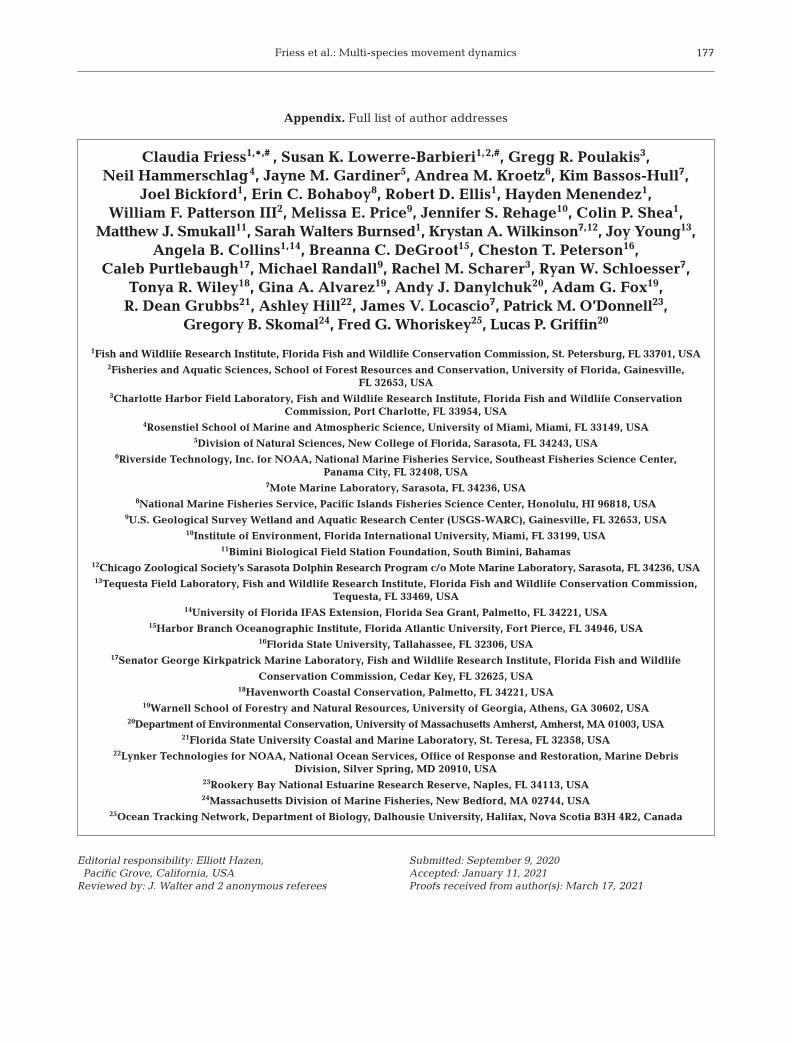
Friess et al.: Multi-species movement dynamics 177

Editorial responsibility: Elliott Hazen, Pacific Grove, California, USA

Reviewed by: J. Walter and 2 anonymous referees

Submitted: September 9, 2020Accepted: January 11, 2021Proofs received from author(s): March 17, 2021

Appendix. Full list of author addresses

Claudia Friess1,*,# , Susan K. Lowerre-Barbieri1,2,#, Gregg R. Poulakis3, Neil Hammerschlag4, Jayne M. Gardiner5, Andrea M. Kroetz6, Kim Bassos-Hull7,

Joel Bickford1, Erin C. Bohaboy8, Robert D. Ellis1, Hayden Menendez1, William F. Patterson III2, Melissa E. Price9, Jennifer S. Rehage10, Colin P. Shea1,

Matthew J. Smukall11, Sarah Walters Burnsed1, Krystan A. Wilkinson7,12, Joy Young13, Angela B. Collins1,14, Breanna C. DeGroot15, Cheston T. Peterson16,

Caleb Purtlebaugh17, Michael Randall9, Rachel M. Scharer3, Ryan W. Schloesser7,Tonya R. Wiley18, Gina A. Alvarez19, Andy J. Danylchuk20, Adam G. Fox19,

R. Dean Grubbs21, Ashley Hill22, James V. Locascio7, Patrick M. O’Donnell23, Gregory B. Skomal24, Fred G. Whoriskey25, Lucas P. Griffin20

1Fish and Wildlife Research Institute, Florida Fish and Wildlife Conservation Commission, St. Petersburg, FL 33701, USA2Fisheries and Aquatic Sciences, School of Forest Resources and Conservation, University of Florida, Gainesville,

FL 32653, USA3Charlotte Harbor Field Laboratory, Fish and Wildlife Research Institute, Florida Fish and Wildlife Conservation

Commission, Port Charlotte, FL 33954, USA4Rosenstiel School of Marine and Atmospheric Science, University of Miami, Miami, FL 33149, USA

5Division of Natural Sciences, New College of Florida, Sarasota, FL 34243, USA6Riverside Technology, Inc. for NOAA, National Marine Fisheries Service, Southeast Fisheries Science Center,

Panama City, FL 32408, USA7Mote Marine Laboratory, Sarasota, FL 34236, USA

8National Marine Fisheries Service, Pacific Islands Fisheries Science Center, Honolulu, HI 96818, USA9U.S. Geological Survey Wetland and Aquatic Research Center (USGS-WARC), Gainesville, FL 32653, USA

10Institute of Environment, Florida International University, Miami, FL 33199, USA11Bimini Biological Field Station Foundation, South Bimini, Bahamas

12Chicago Zoological Society’s Sarasota Dolphin Research Program c/o Mote Marine Laboratory, Sarasota, FL 34236, USA13Tequesta Field Laboratory, Fish and Wildlife Research Institute, Florida Fish and Wildlife Conservation Commission,

Tequesta, FL 33469, USA14University of Florida IFAS Extension, Florida Sea Grant, Palmetto, FL 34221, USA

15Harbor Branch Oceanographic Institute, Florida Atlantic University, Fort Pierce, FL 34946, USA16Florida State University, Tallahassee, FL 32306, USA

17Senator George Kirkpatrick Marine Laboratory, Fish and Wildlife Research Institute, Florida Fish and Wildlife

Conservation Commission, Cedar Key, FL 32625, USA18Havenworth Coastal Conservation, Palmetto, FL 34221, USA

19Warnell School of Forestry and Natural Resources, University of Georgia, Athens, GA 30602, USA20Department of Environmental Conservation, University of Massachusetts Amherst, Amherst, MA 01003, USA

21Florida State University Coastal and Marine Laboratory, St. Teresa, FL 32358, USA22Lynker Technologies for NOAA, National Ocean Services, Office of Response and Restoration, Marine Debris

Division, Silver Spring, MD 20910, USA23Rookery Bay National Estuarine Research Reserve, Naples, FL 34113, USA24Massachusetts Division of Marine Fisheries, New Bedford, MA 02744, USA

25Ocean Tracking Network, Department of Biology, Dalhousie University, Halifax, Nova Scotia B3H 4R2, Canada