1

Regional Rice Initiative (RRI) Policy Simulation to Alleviate Climate Risks of Rice Production System and Rice Market

FINAL TECHNICAL REPORT

I. Background

The FAO-supported Regional Rice Initiative (RRI) Project started in May 2013 and its overall objective is to (i) promote the importance of goods/services produced by and available from rice ecosystems and (ii) identify sustainable rice production practices to improve food security. The participating countries for the RRI project are the Philippines, Laos and Indonesia. The RRI has four different Components:

1. Component 1 – conduct assessments of ecosystem services produced by fisheries and aquaculture within rice-field production systems, and improve water management practices that are able to take into account the changing irrigation and drainage services required by farmers for the adoption of sustainable management practices in dynamic economic and water resources settings.

2. Component 2 - build knowledge and capacity in the form of tools, training and analysis

for integrated management of biodiversity, landscapes and ecosystem services to enhance sustainability in rice ecosystems, including studies of “Trees outside Forests”, or trees in rice fields.

3. Component 3 – focus on capacity building of famers adopting and practicing “Save and

Grow” and sustainable intensification of rice production through Farmer Field Schools (FFS).

4. Component 4 – develop information and knowledge products for policy makers to better

manage climate risks in the rice sector and to identify adaptation needs for the rice sector with support from the AMICAF (Analysis and Mapping of Impacts under Climate Change for Adaptation and Food Security) project. This component also promotes understanding and awareness of the importance of paddy ecosystems, associated knowledge systems, biodiversity, landscapes and cultures through the Globally Important Agricultural Heritage Systems (GIAHS) Initiative.

The NEDA is a partner agency under Component 4. The NEDA component started in 17 September 2013 and was completed on 31 December 2014.

II. Project Objectives

The NEDA component under the RRI Project aims to conduct a policy simulation on the impact of climate change on the Philippine rice market using the Provincial Agricultural Market (PAM) Model developed under the AMICAF Project.

2

III. Methodology A. Overall Methodology

Similar to the approach under the AMICAF project, the impact (e.g. elasticity) of the policy variable to rice yield was estimated first by using a separate regression model. Afterwards, the percentage change in yield due to the impact of the policy variable is inputted to the PAM model (i.e. treated exogenously) to conduct the policy simulation. The level of public expenditure on agriculture was considered as the policy variable since a long time-series data is already available at Bureau of Agricultural Statistics of the Philippine Statistical Authority (PSA-BAS).

B. Development of Regression Model 1. Overview of Regression Model

a. The regression model was estimated with two (2) behavioural equations1 and one

(1) identity equation2.

b. The model parameters were estimated using Ordinary Least Squares (OLS) Regression on 1981-2010 time series data from PSA-BAS (for rice data) and PAGASA (for climate variables).

c. The estimated parameters provide the impact of government agriculture

expenditure, maximum temperature, minimum temperature and precipitation on rice yield by ecosystem for 1981-2010.

d. The regression model was used to make a projection of future irrigated rice yield up

to year 2030 assuming that the government agriculture expenditure will increase by 5% annually in 2011-2030.

e. The percentage change in future irrigated rice yield was inputted in the PAM model to conduct the policy simulation under this study.

2. Description of Variables Used

The list of data, source and name of variables used in the development of the regression

model is presented in Table 1 below. The policy variable used is the level of government

expenditure on agriculture expressed as a ratio versus the total government expenditure.

The time series data on government expenditure on agriculture was sourced from the PSA-

BAS3. The climate variables used on maximum temperature, minimum temperature and

precipitation were sourced from the projection of PAGASA under the AMICAF Project.

1 A behavioural equation is an equation that was estimated from historical data and contains an error term which accounts for the effect of other factors not included in the equation. 2An identity equation refers to an equation that is true by definition. 3 There is no long time-series data on public expenditure on rice only covering 1981-2010. The simulation under this study assumes that a large portion of public expenditure on agriculture has been devoted to rice.

3

Table 1. List of Data and Name of Variable Used

Source: NEDA-ANRES

3. Specification of the Regression Model

There are separate equations for irrigated and rainfed yield since the impact of climate

variables may differ by ecosystem as follow:

Equation 1 is the irrigated yield equation as a function of the ratio of government

expenditure on agriculture versus its total expenditure, farmgate price lagged by one (1)

year, maximum temperature, minimum temperature and u is the error term.

Equation 2 is the rainfed yield equation as a function of farmgate price lagged by one (1)

year, precipitation, maximum temperature and minimum temperature and v is the error

term.

According to a draft study by Habito et al in 2011 entitled Fostering our Farms, Fisheries and Food, about 60%-70% of the DA’s budget was spent on rice.

4

Equation 3 computes for the total yield and it is the weighted average of irrigated and

rainfed yield from Equation 1 and Equation 2, respectively, with the weights computed

based on area harvested.

The hypothesis is that tmax and tmin have a negative impact on both irrigated and rainfed

yield, while precipitation has a positive impact on rainfed yield4. The term “dlog” means the

difference in logarithm of the variables which is equivalent to expressing them in growth

rates. The variables were expressed in difference in logarithm to address the issue of non-

stationarity5.

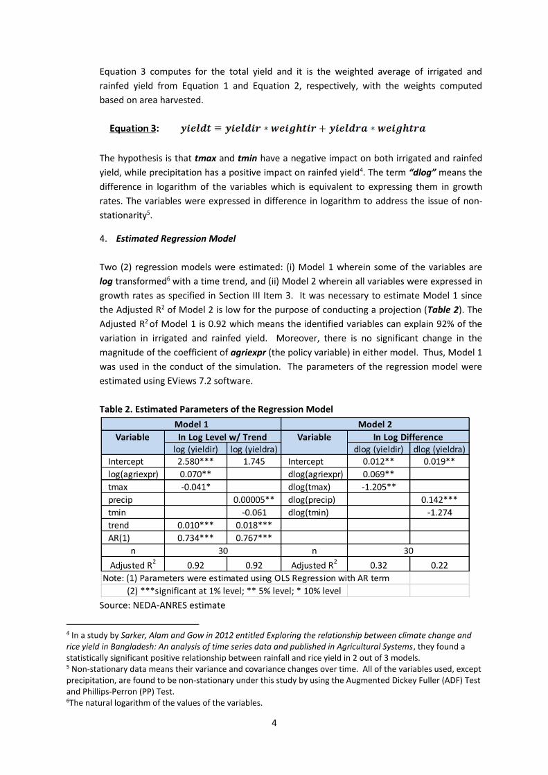
4. Estimated Regression Model

Two (2) regression models were estimated: (i) Model 1 wherein some of the variables are

log transformed6 with a time trend, and (ii) Model 2 wherein all variables were expressed in

growth rates as specified in Section III Item 3. It was necessary to estimate Model 1 since

the Adjusted R2 of Model 2 is low for the purpose of conducting a projection (Table 2). The

Adjusted R2 of Model 1 is 0.92 which means the identified variables can explain 92% of the

variation in irrigated and rainfed yield. Moreover, there is no significant change in the

magnitude of the coefficient of agriexpr (the policy variable) in either model. Thus, Model 1

was used in the conduct of the simulation. The parameters of the regression model were

estimated using EViews 7.2 software.

Table 2. Estimated Parameters of the Regression Model

Source: NEDA-ANRES estimate

4 In a study by Sarker, Alam and Gow in 2012 entitled Exploring the relationship between climate change and rice yield in Bangladesh: An analysis of time series data and published in Agricultural Systems, they found a statistically significant positive relationship between rainfall and rice yield in 2 out of 3 models. 5 Non-stationary data means their variance and covariance changes over time. All of the variables used, except precipitation, are found to be non-stationary under this study by using the Augmented Dickey Fuller (ADF) Test and Phillips-Perron (PP) Test. 6The natural logarithm of the values of the variables.

log (yieldir) log (yieldra) dlog (yieldir) dlog (yieldra)Intercept 2.580*** 1.745 Intercept 0.012** 0.019**

log(agriexpr) 0.070** dlog(agriexpr) 0.069**

tmax -0.041* dlog(tmax) -1.205**

precip 0.00005** dlog(precip) 0.142***

tmin -0.061 dlog(tmin) -1.274

trend 0.010*** 0.018***

AR(1) 0.734*** 0.767***

n n

Adjusted R2 0.92 0.92 Adjusted R2 0.32 0.22

Note: (1) Parameters were estimated using OLS Regression with AR term

(2) ***significant at 1% level; ** 5% level; * 10% level

Model 1 Model 2

Variable

3030

In Log Level w/ Trend In Log DifferenceVariable

5

The ratio of government agriculture expenditure vs. total (agriexpr) was found to be

statistically significant at the 5% level (Table 2). The estimated elasticity of agriexpr is about

0.07 which means that a 1% increase in agriexpr will lead to a 0.07% increase in irrigated

yield. Both maximum and minimum temperature have a negative impact on both irrigated

and rainfed palay yield. However, only maximum temperature is statistically significant.

Precipitation has a small positive impact on rainfed yield and is statistically significant at the

5% level.

5. Diagnostic Tests

Basic diagnostic tests also indicate that the regression model satisfies the tests on normality of residual7, serial correlation8, and heteroskedasticity9 at the 5% level (Table 3). However, there is presence of multicollinearity10 under Model 1 based on the Variance Inflation Factor (VIF)11. Although there is multicollinearity, it does not affect the unbiasedness12 of the estimated parameters in the model. Moreover, Model 1 can make reasonable forecast since the bias and variance proportions of the reported Theil Coefficient are smaller compared to the covariance proportion.

Table 3. Results of Common Diagnostic Test for Regression

Source: NEDA-ANRES

C. Development of the Provincial Agricultural Market (PAM) Model Under the AMICAF Project, a partial equilibrium13 econometric model was developed in partnership with the FAO14 called the “Provincial Agricultural Market” model or PAM. The following are the major features of PAM model:

Uses Microsoft Excel as platform – The MS Excel is common software and less complicated to operate compared to other statistical software (e.g. EViews, Stata, GAMS).

7 The residual is normally distributed 8The error term is related to itself in time 9 The variance is not constant 10 An independent variable is related to other independent variables in the model which makes it hard to estimate their separate effects. 11A VIF of more than 10 indicates the presence of multicollinearity. 12Unbiasedness means that the estimated coefficients are equal to the true population parameters on average. 13 A partial equilibrium model focuses on one or more sectors of the economy and assumes that changes in other sectors are negligible. 14 The PAM was developed by Dr.Tatsuji Koizumi of the FAO.

1) Normality of Residual Jarque-Bera 0.59 (p-value) 0.75 (p-value) 0.68 (p-value) 0.71 (p-value)

2) Serial Correlation Breusch-Godfrey 0.35 (p-value) 0.61 (p-value) 0.82 (p-value) 0.64 (p-value)

3) Heteroskedasticity Breusch-Pagan-Godfrey 0.33 (p-value) 0.07 (p-value) 0.73 (p-value) 0.27 (p-value)

Variance Inflation Factoryes for tmax

(uncentered VIF)

yes for tmin

(uncentered VIF)

none (VIF is less

than 10)

none (VIF is less

than 10)

Bias Proportion 0.02 0.00 0.39 0.00

Variance Proportion 0.21 0.06 0.00 0.06

Covariance Proportion 0.77 0.94 0.60 0.94

4) Multicollinearity

5) Theil Coefficient

In Log Difference

Model 1 Model 2Item Test/Criteria

In Log Level w/ Trend

6

Commodity coverage – The focus commodity is irrigated rice and rainfed rice.

Spatial coverage – The model is disaggregated by province.

Timeframe of projection – From year 2011 to year 2030.

Major variables in projection – Irrigated rice production, rainfed rice production, irrigated rice area harvested, rainfed rice area harvested and farmgateprices.

1. Linkage of the PAM Model with other Step 1 AMICAF Models

The PAM model is not a stand-alone model, but is linked with other models of other partner agencies under Step 1 of the AMICAF Project (Figure 1). This partnership between different agencies and linkage between various models enables a multi-disciplinary approach in assessing the different impacts of Climate Change.

Figure 1. Linkage of the PAM Model with other Step 1 Models

Source: NEDA-ANRES First, the PAGASA conducted a downscaling of the projected minimum temperature, maximum temperature and precipitation of three (3) Global Circulation Models (GCM) namely: (i) Bergen Climate Model (BCM) from Norway, (ii) Centre National de Recherches Meteorologiques (CNCM3) from France, and (iii) Max-Planck-Institute for Meteorology (MPEH5) from Germany. Two (2) climate change scenarios were used by each GCM: (i) A1B Scenario and (ii) A2 Scenario. The A1B Scenario is a medium-range emission scenario characterized by a balance in the use of both fossil and non-fossil fuel, while the A2 Scenario is a high-range emission scenario focused on regionally-oriented economic development in the future. The emission scenarios are based on the Special Report on Emissions Scenarios (SRES) by the Intergovernmental Panel on Climate Change (IPCC) published in 2000. These projections of climate variables were then used by the PhilRice to conduct a projection of future irrigated and rainfed rice yield, and by the UP-NIGS to conduct a projection of future water discharge (or availability) in major river basins in the Philippines from 2011 to 2030. The projections of PhilRice on rice yield and UP-NIGS on water discharge are integral inputs to the PAM Model under the NEDA component. The projected yields and water discharges

7

are used in the computation of area harvested and total rice production to come up with projected rice prices in 2011-2030.

2. Framework of the PAM Model with Policy Variable

The PAM model computes an equilibrium price (farmgate) that balances the supply and demand of rice in the market (Figure 2). The supply of rice is composed of domestic production, import and beginning stocks. The demand for rice, on the other hand, is composed of food demand, demand for seeds, feeds, waste and processing as well as ending stocks.

Figure 2. Framework of the PAM Model with Policy Variable

Source: NEDA-ANRES

An increase in the supply of rice relative to demand, will lead to a decrease in prices, while an increase in the demand of rice relative to supply, will lead to an increase in prices15. The policy variable such as public expenditure on agriculture affects yield which in turn will affect domestic rice production.

The most important component of rice supply is domestic production. It is computed as the product between the yield projections from the Crop Model of PhilRice and area harvested. The area harvested in the PAM model is affected by water availability from the projection of UP-NIGS. On the other hand, the bulk of rice demand comes from food demand which in turn is affected by per capita income and population growth.

3. Major Equations of the PAM Model

a. Equation for Irrigated Rice Production. Irrigated palay production is computed, by

province, as the product between irrigated yield and area harvested. It is converted to milled terms by using the standard conversion factor of 0.654.

15with the assumption of ceteris paribus or all else equal.

8

𝐼𝑟𝑟𝑖𝑔𝑎𝑡𝑒𝑑 𝑃𝑟𝑜𝑑𝑢𝑐𝑡𝑖𝑜𝑛 = 𝐼𝑟𝑟𝑖𝑔𝑎𝑡𝑒𝑑 𝑌𝑖𝑒𝑙𝑑 ∗ 𝐴𝑟𝑒𝑎 𝐻𝑎𝑟𝑣𝑒𝑠𝑡𝑒𝑑 (1.1)

b. Equation for Irrigated Area Harvested. Irrigated area harvested is computed as a

function of farmgate price. The magnitude of the change depends on the value of the elasticity of irrigated area harvested with respect to rice price. The elasticity is a positive number and it varies in each province which was estimated by using Ordinary Least Squares (OLS) Regression.

𝐼𝑟𝑟𝑖𝑔𝑎𝑡𝑒𝑑 𝐴𝑟𝑒𝑎 𝐻𝑎𝑟𝑣𝑒𝑠𝑡𝑒𝑑

= 𝐴𝑟𝑒𝑎 𝐻𝑎𝑟𝑣𝑒𝑠𝑡𝑒𝑑𝑡−1 ∗ (𝑓𝑎𝑟𝑚𝑔𝑎𝑡𝑒 𝑝𝑟𝑖𝑐𝑒𝑡

𝑓𝑎𝑟𝑚𝑔𝑎𝑡𝑒 𝑝𝑟𝑖𝑐𝑒𝑡−1

)^𝑟𝑖𝑐𝑒 𝑝𝑟𝑖𝑐𝑒 𝑒𝑙𝑎𝑠𝑡𝑖𝑐𝑖𝑡𝑦

(1.2)

c. Equation for Rainfed Rice Production. Rainfed palay production is computed, by

province, as the product between rainfed yield and area harvested. It is converted to milled terms by using the standard conversion factor of 0.654.

𝑅𝑎𝑖𝑛𝑓𝑒𝑑 𝑃𝑟𝑜𝑑𝑢𝑐𝑡𝑖𝑜𝑛 = 𝑅𝑎𝑖𝑛𝑓𝑒𝑑 𝑌𝑖𝑒𝑙𝑑 ∗ 𝐴𝑟𝑒𝑎 𝐻𝑎𝑟𝑣𝑒𝑠𝑡𝑒𝑑 (1.3)

d. Equation for Rainfed Area Harvested. Rainfed area harvested is computed as a

function of farmgate price and corn price. The magnitude of the change depends on the value of the elasticity of rainfed area harvested with respect to rice price and corn price. The elasticities vary in each province and were estimated using Ordinary Least Squares (OLS) Regression.

𝑅𝑎𝑖𝑛𝑓𝑒𝑑 𝐴𝑟𝑒𝑎 𝐻𝑎𝑟𝑣𝑒𝑠𝑡𝑒𝑑

= 𝐴𝑟𝑒𝑎 𝐻𝑎𝑟𝑣𝑒𝑠𝑡𝑒𝑑𝑡−1

∗ ((𝑓𝑎𝑟𝑚𝑔𝑎𝑡𝑒 𝑝𝑟𝑖𝑐𝑒𝑡

𝑓𝑎𝑟𝑚𝑔𝑎𝑡𝑒 𝑝𝑟𝑖𝑐𝑒𝑡−1

)^𝑟𝑖𝑐𝑒 𝑝𝑟𝑖𝑐𝑒 𝑒𝑙𝑎𝑠𝑡𝑖𝑐𝑖𝑡𝑦

∗ (𝑐𝑜𝑟𝑛 𝑝𝑟𝑖𝑐𝑒𝑡

𝑐𝑜𝑟𝑛 𝑝𝑟𝑖𝑐𝑒𝑡−1

)^𝑐𝑜𝑟𝑛 𝑝𝑟𝑖𝑐𝑒 𝑒𝑙𝑎𝑠𝑡𝑖𝑐𝑖𝑡𝑦

)

(1.4)

e. Equation for per capita consumption. The per capita consumption (PCC) for rice is

computed as a function of per capita Gross Domestic Product (GDP), rice retail price and corn retail price (substitute commodity). The income elasticity used is 0.23, rice price elasticity is -0.24 and corn price elasticity is 0.15. The PCC is computed at the national level.

𝑃𝐶𝐶 = 𝑃𝐶𝐶𝑡−1 ∗ ((𝑝𝑐 𝐺𝐷𝑃𝑡

𝑝𝑐 𝐺𝐷𝑃𝑡−1

)^(0.23)𝑖𝑛𝑐𝑜𝑚𝑒 𝑒𝑙𝑎𝑠𝑡𝑖𝑐𝑖𝑡𝑦

∗ (𝑟𝑖𝑐𝑒 𝑟𝑒𝑡𝑎𝑖𝑙 𝑝𝑟𝑖𝑐𝑒𝑡

𝑟𝑖𝑐𝑒 𝑟𝑒𝑡𝑎𝑖𝑙 𝑝𝑟𝑖𝑐𝑒𝑡−1

)^(−0.24)𝑟𝑖𝑐𝑒 𝑝𝑟𝑖𝑐𝑒 𝑒𝑙𝑎𝑠𝑡𝑖𝑐𝑖𝑡𝑦

∗ (𝑐𝑜𝑟𝑛 𝑟𝑒𝑡𝑎𝑖𝑙 𝑝𝑟𝑖𝑐𝑒𝑡

𝑐𝑜𝑟𝑛 𝑟𝑒𝑡𝑎𝑖𝑙 𝑝𝑟𝑖𝑐𝑒𝑡−1

)^(0.15)𝑐𝑜𝑟𝑛 𝑝𝑟𝑖𝑐𝑒 𝑒𝑙𝑎𝑠𝑡𝑖𝑐𝑖𝑡𝑦

)

(1.5)

9

f. Equation for food consumption. The total food consumption or demand is computed as a product between PCC and population. The total food consumption is computed at the national level.

𝐹𝑜𝑜𝑑 𝐶𝑜𝑛𝑠𝑢𝑚𝑝𝑡𝑖𝑜𝑛 = 𝑃𝐶𝐶 ∗ 𝑃𝑜𝑝𝑢𝑙𝑎𝑡𝑖𝑜𝑛 (1.6)

g. Equation for imports. The level of imports is computed as a function of the wholesale price of rice and the world price of rice. The world price of rice is an exogenous variable taken from the Rice Economy Climate Change (RECC) Model16. The RECC Model is an international model covering rice markets in 15 countries and generates world price projections under Climate Change. The rice price elasticity used is -0.10 and the world price elasticity is -0.44. This means that increases in the wholesale and world prices for rice will lead to a decline in the level of imports. The level of imports is computed at the national level.

𝐼𝑚𝑝𝑜𝑟𝑡𝑠 = 𝐼𝑚𝑝𝑜𝑟𝑡𝑠𝑡−1

∗ ((𝑤ℎ𝑜𝑙𝑒𝑠𝑎𝑙𝑒 𝑝𝑟𝑖𝑐𝑒𝑡

𝑤ℎ𝑜𝑙𝑒𝑠𝑎𝑙𝑒 𝑝𝑟𝑖𝑐𝑒𝑡−1

)(^−0.10)𝑟𝑖𝑐𝑒 𝑝𝑟𝑖𝑐𝑒 𝑒𝑙𝑎𝑠𝑡𝑖𝑐𝑖𝑡𝑦

∗ (𝑤𝑜𝑟𝑙𝑑 𝑝𝑟𝑖𝑐𝑒𝑡

𝑤𝑜𝑟𝑙𝑑 𝑝𝑟𝑖𝑐𝑒𝑡−1

)^(−0.44)𝑤𝑜𝑟𝑙𝑑 𝑝𝑟𝑖𝑐𝑒 𝑒𝑙𝑎𝑠𝑡𝑖𝑐𝑖𝑡𝑦

)

(1.7)

h. Equation for ending stocks. The ending stock of rice is a function of rice consumption. The magnitude of change depends on the value of the elasticity of ending stocks with respect to rice food consumption. The elasticity used is -0.05 which means that an increase in rice food consumption will lead to a decrease in ending stocks for rice.

𝐸𝑛𝑑𝑖𝑛𝑔 𝑆𝑡𝑜𝑐𝑘𝑠 = 𝐸𝑛𝑑𝑖𝑛𝑔 𝑆𝑡𝑜𝑐𝑘𝑠𝑡−1

∗ ((𝑟𝑖𝑐𝑒 𝑓𝑜𝑜𝑑 𝑐𝑜𝑛𝑠𝑢𝑚𝑝𝑡𝑖𝑜𝑛𝑡

𝑟𝑖𝑐𝑒 𝑓𝑜𝑜𝑑 𝑐𝑜𝑛𝑠𝑢𝑚𝑝𝑡𝑖𝑜𝑛𝑡−1

)^(−0.05)𝑟𝑖𝑐𝑒 𝑐𝑜𝑛𝑠𝑢𝑚𝑝𝑡𝑖𝑜𝑛 𝑒𝑙𝑎𝑠𝑡𝑖𝑐𝑖𝑡𝑦

) (1.8)

i. Equation for wholesale price. The wholesale price of rice is computed as a function of farmgate price. The magnitude of change depends on the value of the elasticity of wholesale price with respect to farmgate price. The elasticity used is 0.92 and was estimated using OLS Regression.

𝑊ℎ𝑜𝑙𝑒𝑠𝑎𝑙𝑒 𝑃𝑟𝑖𝑐𝑒 = 𝑊ℎ𝑜𝑙𝑒𝑠𝑎𝑙𝑒 𝑃𝑟𝑖𝑐𝑒𝑡−1 ∗ ((𝐹𝑎𝑟𝑚𝑔𝑎𝑡𝑒 𝑃𝑟𝑖𝑐𝑒𝑡

𝐹𝑎𝑟𝑚𝑔𝑎𝑡𝑒 𝑃𝑟𝑖𝑐𝑒𝑡−1

)^(0.92) 𝑟𝑖𝑐𝑒 𝑝𝑟𝑖𝑐𝑒 𝑒𝑙𝑎𝑠𝑡𝑖𝑐𝑖𝑡𝑦

) (1.9)

j. Equation for retail price. The retail price of rice is computed as a function of farmgate price. The magnitude of change depends on the value of the elasticity of retail price with respect to farmgate price. The elasticity used is 0.99 and was estimated using OLS Regression.

𝑅𝑒𝑡𝑎𝑖𝑙 𝑃𝑟𝑖𝑐𝑒 = 𝑅𝑒𝑡𝑎𝑖𝑙 𝑃𝑟𝑖𝑐𝑒𝑡−1 ∗ ((𝐹𝑎𝑟𝑚𝑔𝑎𝑡𝑒 𝑃𝑟𝑖𝑐𝑒𝑡

𝐹𝑎𝑟𝑚𝑔𝑎𝑡𝑒 𝑃𝑟𝑖𝑐𝑒𝑡−1

)^(0.99)𝑟𝑖𝑐𝑒 𝑝𝑟𝑖𝑐𝑒 𝑒𝑙𝑎𝑠𝑡𝑖𝑐𝑖𝑡𝑦

) (1.10)

16 The RECC was developed by Dr.Tatsuji Koizumi of the FAO

10

k. Equation for farmgate price. The farmgate price is computed as the price level that balances the supply and demand of rice in the market. This equilibrium farmgate price is computed in the PAM using the Gauss-Seidel Algorithm by balancing the following equation.

𝑃𝑟𝑜𝑑𝑢𝑐𝑡𝑖𝑜𝑛 + 𝐼𝑚𝑝𝑜𝑟𝑡𝑠 + 𝐵𝑒𝑔. 𝑆𝑡𝑜𝑐𝑘𝑠

= 𝐹𝑜𝑜𝑑 𝐶𝑜𝑛𝑠𝑢𝑚𝑝𝑡𝑖𝑜𝑛 + 𝑆𝑒𝑒𝑑𝑠, 𝑒𝑡𝑐. +𝐸𝑛𝑑 𝑆𝑡𝑜𝑐𝑘𝑠 (1.11)

4. Data Used

a. GDP – NEDA (2014: 6.5%, 2015: 7.0%, 2016: 7.5%) and ADB (2017-2030: 5.6%) projections17.

b. Population – PSA-NSCB (2011-2020: 1.8%) and ADB (2021-2030: 1.4%) projections18. c. World price of rice – Projection of the Rice Economy Climate Change (RECC) Model.

The RECC Model is an international partial equilibrium model covering rice markets in 15 countries and generates world price projections under Climate Change.

d. White corn prices – Historical farmgate price from PSA-BAS. The projection in 2011-2030 was computed by using exponential smoothing method (additive) with the root mean square error (RMSE) as criteria.

e. Per capita consumption – 2008-2009 Survey on Food Demand (SFD) by PSA-BAS f. Irrigated and Rainfed Rice Yield – Projection from the PhilRiceCrop Model g. Water Availability – Projection from the UP-NIGS Hydrology Model

h. Baseline data – Baseline data on rice production, area harvested, prices, imports,

stocks and utilization for seeds, feeds & waste, and processing from PSA-BAS.

17 Asian Development Bank, 2011. Long-Term Projection of Asian GDP and Trade. 18 Ibid

11

IV. Results and Discussion 1. Assumptions by Scenario. The policy simulation using the PAM model was conducted by

assuming that irrigated yield will increase by 1.85% on the average due to a 5% annual increase in government agriculture expenditure in 2011-2030 (Table 4). The future increase in irrigated yield was projected using the regression model (Section III, Item B) with an estimated elasticity of irrigated rice yield with respect to the ratio of government agriculture expenditure vs. total expenditure of 0.07.

Table 4. Assumptions by Scenario for all GCM’s and Climate Scenarios

Item Assumption

Yield (in MT per hectare)

Base: Irrigated rice yield from PhilRice with Climate Change Scenario: 1.85% increase in irrigated rice yield due to 5% annual increase in government agriculture expenditure in 2011-2030 (projection using the regression model in Section III, Item B).

Source: Irrigated yield from PhilRice under AMICAF Project

2. Increasing the annual government expenditure on agriculture will increase domestic rice

production. Based on the average of the 3 GCMs, increasing government expenditure on agriculture by 5% annually in 2011-2030 will increase rice production from 18.23 MMT to 18.32 MMT or an increase of 0.49% under the A1B scenario (Table 5). The same trend is also observed under the A2 scenario. It should be noted that the increase in rice production is small since the estimated elasticity is also small at 0.07. This is included as a limitation of this study.

Table 5. Policy Simulation on Rice Production using PAM, 2011-2030

Source: NEDA-ANRES estimate

2026-2030 2011-2030 2026-2030 2011-2030

BCM2

Base

Production 20,051,810 18,219,269 20,149,405 18,271,459

Scenario

Production 20,146,331 18,308,724 20,244,783 18,361,297

CNCM3

Base

Production 20,092,749 18,193,216 20,256,070 18,261,476

Scenario

Production 20,187,083 18,282,047 20,352,393 18,350,890

MPEH5

Base

Production 20,171,416 18,278,796 20,147,284 18,214,459

Scenario

Production 20,265,898 18,368,527 20,242,956 18,304,274

Average of 3 GCMs

Base 20,105,325 18,230,427 20,184,253 18,249,131

Scenario 20,199,771 18,319,766 20,280,044 18,338,820

% change 0.47 0.49 0.47 0.49

Global Circulation

Models

PAM Model Policy Simulation (2011-2030)

A1B Scenario A2 Scenario

12

3. The increase in domestic rice production will lower farmgate prices by reducing the demand-supply deficit. Based on the average of the 3 GCMs, increasing government expenditure on agriculture by 5% annually in 2011-2030 will lower farmgate prices from Php 23.27 per kilo to Php 22.79 per kilo or a decrease of -2.06% under A1B scenario (Table 6). The result is almost similar under the A2 scenario with farmgate prices projected to decrease by -2.07% on the average in the same period. This is due to higher rice production as a result of an increase in government expenditure on agriculture, which will lead to a lower demand-supply deficit and eventually lower farmgate prices.

Table 6. Policy Simulation on Rice Farmgate Price using PAM, 2011-2030

Source: NEDA-ANRES estimate

V. Limitation and Future Study

1. The impact of the policy variable on rice yield is exogenous from another model. The elasticity of irrigated yield with respect to government expenditure on agriculture was estimated from a separate model since the PAM has no built-in policy variable. This raises the issue if the analysis is done under a consistent framework.

2. The estimated elasticity used in the policy simulation is small. The magnitude of the estimated elasticity of irrigated yield with respect to government expenditure on agriculture of 0.07 is quite small based on the regression model using 1981-2010 time series data. Using panel data may result to a better estimate but this study is constrained by time and lack of disaggregated public expenditure data on agriculture at the provincial level to conduct such analysis.

2026-2030 2011-2030 2026-2030 2011-2030

BCM2

Base

Farmgate Price 30.199 23.342 29.573 23.062

Scenario

Farmgate Price 29.583 22.859 28.968 22.585

CNCM3

Base

Farmgate Price 29.927 23.484 28.927 23.068

Scenario

Farmgate Price 29.319 23.001 28.332 22.592

MPEH5

Base

Farmgate Price 29.430 22.980 29.594 23.317

Scenario

Farmgate Price 28.834 22.505 28.986 22.833

Average of 3 GCMs

Base 29.852 23.268 29.365 23.149

Scenario 29.245 22.788 28.762 22.670

% change -2.03 -2.06 -2.05 -2.07

Global Circulation

Models

PAM Model Policy Simulation (2011-2030)

A1B Scenario A2 Scenario

13

VI. Conclusion and Recommendation

1. Government intervention is important to address the negative impact of climate change on future rice production and farmgate prices. The policy simulation shows that increasing the expenditure of the government on agriculture can increase rice production in 2011-2030 (by 0.49%) which will contribute in lowering the demand-supply deficit and thereby lowering future farmgate prices (by -2.1%). Lower farmgate prices will also lead to lower retail prices and will benefit rice consumers especially the poor who spent 20% of their total food expenditure on rice.

2. The results of the policy simulation can be further improved by incorporating policy variables directly to the PAM model and using other methods to estimate the historical impact of such policy variables. This will ensure that the policy simulation is done under a more consistent framework. Using other methods, such as regression using panel data, may yield more robust estimates of the impact of policy variables on rice yield which will further enhance the results of the simulation.

14

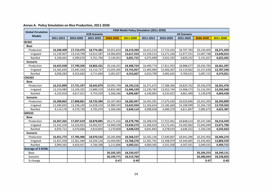
Annex A. Policy Simulation on Rice Production, 2011-2030

2011-2015 2016-2020 2021-2025 2026-2030 2011-2030 2011-2015 2016-2020 2021-2025 2026-2030 2011-2030

BCM2

Base

Production 16,340,409 17,710,475 18,774,381 20,051,810 18,219,269 16,415,214 17,723,432 18,797,783 20,149,405 18,271,459

Irrigated 12,239,967 13,310,799 14,012,587 14,906,859 13,617,553 12,339,515 13,271,240 13,977,551 15,007,748 13,649,014

Rainfed 4,100,441 4,399,676 4,761,794 5,144,951 4,601,715 4,075,699 4,452,192 4,820,232 5,141,657 4,622,445

Scenario

Production 16,423,928 17,799,206 18,865,431 20,146,331 18,308,724 16,499,774 17,811,953 18,888,677 20,244,783 18,361,297

Irrigated 12,365,645 13,445,543 14,153,737 15,055,305 13,755,057 12,465,984 13,406,307 14,119,062 15,157,630 13,787,246

Rainfed 4,058,283 4,353,663 4,711,694 5,091,027 4,553,667 4,033,790 4,405,645 4,769,615 5,087,153 4,574,051

CNCM3

Base

Production 16,315,899 17,721,337 18,642,879 20,092,749 18,193,216 16,371,675 17,588,396 18,829,762 20,256,070 18,261,476

Irrigated 12,159,989 13,104,325 13,889,319 14,832,483 13,496,529 12,230,783 13,052,744 13,968,273 15,116,391 13,592,048

Rainfed 4,155,910 4,617,012 4,753,559 5,260,266 4,696,687 4,140,892 4,535,652 4,861,490 5,139,678 4,669,428

Scenario

Production 16,398,862 17,808,861 18,733,384 20,187,083 18,282,047 16,455,291 17,675,030 18,920,846 20,352,393 18,350,890

Irrigated 12,284,692 13,238,140 14,028,310 14,980,593 13,632,934 12,356,634 13,185,660 14,108,999 15,266,720 13,729,503

Rainfed 4,114,170 4,570,720 4,705,074 5,206,490 4,649,114 4,098,658 4,489,370 4,811,847 5,085,673 4,621,387

MPEH5

Base

Production 16,367,265 17,697,619 18,878,885 20,171,416 18,278,796 16,308,476 17,553,461 18,848,614 20,147,284 18,214,459

Irrigated 12,331,554 13,226,953 14,062,027 14,900,558 13,630,273 12,266,633 13,175,441 14,202,062 15,043,049 13,671,796

Rainfed 4,035,712 4,470,666 4,816,859 5,270,858 4,648,524 4,041,843 4,378,019 4,646,552 5,104,236 4,542,663

Scenario

Production 16,451,772 17,785,906 18,970,532 20,265,898 18,368,527 16,392,136 17,640,907 18,941,096 20,242,956 18,304,274

Irrigated 12,457,430 13,361,449 14,204,134 15,050,092 13,768,276 12,391,791 13,308,979 14,344,065 15,193,401 13,809,559

Rainfed 3,994,342 4,424,457 4,766,398 5,215,806 4,600,251 4,000,345 4,331,928 4,597,031 5,049,555 4,494,715

Average of 3 GCMs

Base 20,105,325 18,230,427 20,184,253 18,249,131

Scenario 20,199,771 18,319,766 20,280,044 18,338,820

% change 0.47 0.49 0.47 0.49

Global Circulation

Models

PAM Model Policy Simulation (2011-2030)

A1B Scenario A2 Scenario

15

Annex B. Policy Simulation on Rice Farmgate Prices, 2011-2030

2011-2015 2016-2020 2021-2025 2026-2030 2011-2030 2011-2015 2016-2020 2021-2025 2026-2030 2011-2030

BCM2

Base

Farmgate Price 16.853 20.877 25.438 30.199 23.342 16.552 20.825 25.297 29.573 23.062

Scenario

Farmgate Price 16.500 20.440 24.915 29.583 22.859 16.203 20.391 24.778 28.968 22.585

CNCM3

Base

Farmgate Price 16.944 20.817 26.247 29.927 23.484 16.715 21.519 25.111 28.927 23.068

Scenario

Farmgate Price 16.590 20.388 25.706 29.319 23.001 16.364 21.077 24.596 28.332 22.592

MPEH5

Base

Farmgate Price 16.740 20.927 24.821 29.430 22.980 17.003 21.676 24.994 29.594 23.317

Scenario

Farmgate Price 16.386 20.491 24.310 28.834 22.505 16.645 21.225 24.475 28.986 22.833

Average of 3 GCMs

Base 29.852 23.268 29.365 23.149

Scenario 29.245 22.788 28.762 22.670

% change -2.03 -2.06 -2.05 -2.07

Global Circulation

Models

PAM Model Policy Simulation (2011-2030)

A1B Scenario A2 Scenario