Regime Dependent risk threshold

8/18/2019 Regime Dependent risk threshold

http://slidepdf.com/reader/full/regime-dependent-risk-threshold 1/41

Regime-Dependent Sovereign Risk Pricing during

the Euro Crisis∗

Anne-Laure Delatte†, Julien Fouquau‡, Richard Portes§

December 12, 2014

Abstract

We test for regime-dependent dynamics in the sovereign bond mar-kets of European peripheral countries during the debt crisis and explainthem. Our estimates based on a panel smooth threshold regressionmodel during January 2006 to September 2012 show : 1) Peripheralsovereign spreads are subject to significant nonlinear dynamics. 2) Thedeterioration of banking risk changes the way investors price risk of thesovereigns. 3) The spreads of European peripheral countries have beenpriced above their historical values, given fundamentals, because of amplification effects. 4) A key indicator regulators may want to moni-tor to check the sovereign tensions is the premium of financial i-Traxx

CDS indices. 5) The estimated thresholds to trigger the crisis regimeare quite low at less than 200 bp.Key Words : European sovereign crisis, Panel Smooth Threshold Re-gression Models, CDS indices.

J.E.L Classification : E44, F34, G12, H63, C23.

∗Previous versions of this paper were presented at seminars in Federal Reserverveof New York, Bank of England, Banque de France, London Business School, NanterreUniversity, the International Finance, Banking Society 2013 conference and the GraduateInstitute Geneva. We are grateful for comments from seminars participants. We would liketo acknowledge helpful discussions with Vincent Bouvatier, Markus Brunnermeier, IsabelleCouet, Jerome Creel, Darrell Duffie, Linda Goldberg, Frederic Malherbe, Mathiew Plosser,Lisa Pollack, Helene Rey, Giovanni Ricco, Or Shachar and Paolo Surico. This research waspartly supported by a grant from the London Business School RAMD fund and from theEU 7th Framework Program (FP7/ 2007-2013) under grant agreement 266800 (FESSUD).

†CNRS, OFCE, CEPR‡Neoma Business School§London Business School, CEPR

1



1 Introduction

Financial market participants have a particular taste for locutions that de-

scribe the dynamics of asset prices. In 2011, when sovereign spreads for Eu-

ropean peripheral countries successively soared, bond market participants

asserted the presence of a cliff risk , the point at which a small shift in a

bond’s value can have a big impact on its price.1 A similar pattern was

emphasized by policymakers (with different terminology) when they com-

plained about growing mistrust on the part of investors, a fact that drove

self-reinforcing dynamics.2 A way to picture these comments is to say that

the sovereign risk pricing is regime-dependent and subject to threshold ef-

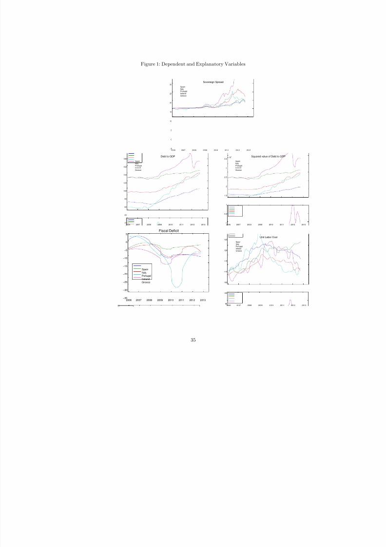
fects. It is clear from the first graph in Fig. 1, which plots spreads between

10-year peripheral and German sovereign bonds, that the trend breaks after

2010, a break that is hard to reconcile with the gradual deterioration of

economic conditions.3

There has been an extensive body of papers examining the sovereign

bond price in the context of the euro crisis and we have learned several im-

portant lessons. First, the massive holding of peripheral sovereign bonds bythe European banking sector created a dangerous nexus between sovereigns

and banks implying feedback loops (Gennaioli et al., 2010, Huizinga and

Demirguc-Kunt, 2010, Acharya and Steffen, 2013, Acharya et al. , 2014,

Coimbra, 2014). Second, adverse liquidity effects on euro area banks have

been documented during the crisis, including a significant fall of inter-bank

loans after mid-2010 (Allen and Moessner, 2013). The four first graphs

in Figure 2, which plot measures of the liquidity premium, indicate that

liquidity conditions in the euro-area did not recover since the sub-prime cri-

1See for example ”Bond investors fear cliff risks.”, Financial Times, November 7, 2011.2”The Greek financial crisis: From Grexit to Grecovery”, Speech by Mr George A

Provopoulos, Governor of the Bank of Greece, for the Golden Series lecture at the Official

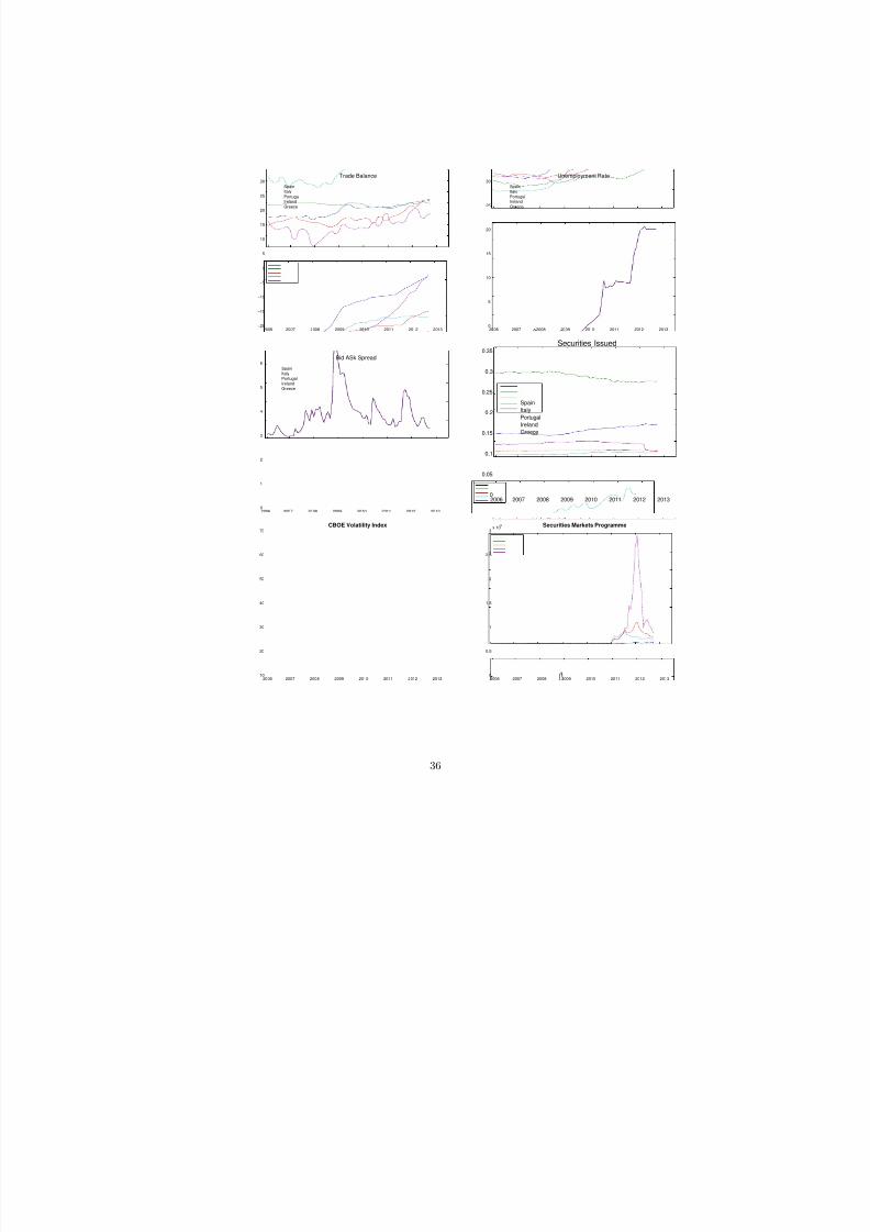
Monetary and Financial Institutions Forum (OMFIF), London, 7 February 2014.3In Spain, for example, the public debt amounted to less than 60% of GDP even by end

2009. The Italian primary budget surplus implied that if interest rates had stayed low, only

modest fiscal adjustment would have been necessary to service the debt. Unemployment

and the trade deficit had b een increasing gradually. And Ireland’s trade balance had been

improving at the time of the crisis.

2



sis, with a clear drop in liquidity from 2011 until the Outright Monetary

Transactions (OMT) measures. Third, previous empirical work document

a regime-switch in the spread determination model for euro-area peripheral

sovereigns during the crisis (Aizenman et al. (2011), Gerlach et al. (2010),

Montfort and Renne (2012), Borgy et al. (2011), Favero and Missale (2011)).

Two different regimes have been described, a crisis and a non-crisis regime,

with additional fundamental factors important in the crisis regime. However

the existing papers do not explain what drove the change in regime.

Here we explore the possibility that initial shocks on economic fundamen-

tals may have been exacerbated by endogenous mechanisms. We can thinkof two potential explanations for self-reinforcing effects: the nexus between

sovereign and bank risk leading to feedback loop effects and liquidity spirals

implying self-amplifying dynamics.

These questions require testing for regime-switching dynamics in bond

spread determination and investigating the triggers. To do so, we use the

smooth transition regression model developed by Terasvirta (1996) and de-

veloped in panel by Gonzalez et al. (2005). Contrary to the alternative

family of nonlinear models, the Markov-switching (MS) models, the STR

model offers a parametric solution to account for nonlinearity by allowing

the parameters to change smoothly as a function of an observable variable

(MS specifications assume that the transition is discrete and the trigger

variable is unobserved). In other words, we take an off-the-shelf model es-

timating the impact of economic fundamentals on the spread of sovereign

bonds, and we consider potential threshold variables to account for the time

variability of the estimated coefficients. We interpret increasing weights in

the spread determination as amplification effects in the sense that the samechange in a fundamental has a higher impact on the spread in the crisis

period than it had previously. Then we follow Gonzalez et al. (2005) to

identify the optimal threshold variable. In sum, our panel threshold regres-

sion framework establishes a ranking among hypotheses that might give rise

to amplification effects (Fouquau et al. 2008). We estimate equations for

the sovereign spreads of five European stress countries: Spain, Ireland, Italy,

Portugal and Greece, over the period January 2006 to September 2012. We

3



deliberately end our sample at the beginning of the OMT programme that

has successfully narrowed the spreads and blurred market signals.4

A preview of our results is the following. We confirm that sovereign

spreads are subject to significant nonlinear dynamics. While we unambigu-

ously detect adverse self-reinforcing liquidity effects, our tests reveal that the

banking-sovereign nexus is the leading driver of nonlinearities. The deteri-

oration of market conditions for financial names changes the way investors

price risk of the sovereigns. We compute the threshold value that triggers

amplification effects in the spreads of the five stress countries, with hetero-geneous dynamics that our PSTR approach enables us to capture.

Our work complements earlier research on sovereign credit risk during

the euro crisis (Acharya et al. 2013, Attinasi et al.2009, Dieckman and

Planck, among others). We show that market liquidity and banking credit

risk not only are significant drivers of sovereign risk but they contribute to it

in a nonlinear manner. They actually exacerbate the effect of initial shocks

to the fundamentals as theory predicts. We show that aggregate financial

variables have a larger impact than country specific variables on the risk-

pricing of domestic debt, a result that emphasizes the issues of maintaining

an incomplete monetary union.

The remainder of this paper is organized as follows. Section 2 reviews

the abundant literature on sovereign bond pricing during the euro-crisis in

order to narrow down our contribution. Section 3 introduces the PSTR

specification methodology and the test procedure. Section 4 summarizes

our data-set, and Section 5 discusses the estimation results. Section 7 sumsup the findings and draw lessons for the economic policy.

4As Paris and Wyplosz (2013) have argued, ”Spreads no longer show us what investors

think about debt sustainability. They reflect a mix of debt-sustainability expectations

and forecasts of ECB reactions”.

4



2 Sovereign risk pricing: what have we learned?

There has been an extensive body of papers examining the sovereign bond

price in the context of the euro crisis. On the one hand, there is a consensus

about a sovereign-banking nexus implying feedback loops in the dynamics

of the sovereign spreads. Acharya et al. (2014) has explicitly modeled the

feedback loop. The deterioration of the sovereign’s creditworthiness feeds

back onto the financial sector, reducing the value of its guarantees and exist-

ing bond holdings and increasing its sensitivity to future sovereign shocks.

On the other hand, bank risk affects the sovereigns, which are expected to

bail out systemically important institutions. That represents a significant

risk given the size of banks compared to the size of the public backstop.

Coimbra (2014) shows how the initial shock is exacerbated and feeds back

to credit conditions. After a rise in sovereign risk, the banks’ VaR constraint

binds, which reduces their demand for sovereign bonds, thereby raising the

sovereign risk premium. This in turn leads to adverse sovereign debt dy-

namics, which raises sovereign risk.

Attinasi et al. (2009) empirically confirm the effect of the bank-sovereignnexus in a model of government bond yield spreads over Germany of 10

European countries. They find that government bond yield spreads are

significantly affected by the announcements of bank rescue packages in ad-

dition to standard measures of government creditworthiness. Acharya et

al.(2013) find that credit default swap (CDS) spreads of banks and those of

governments tend to move more closely together after the announcement of

financial sector bailouts.5

On the other hand, liquidity spirals have played an important role dur-

ing the euro crisis. More precisely liquidity spirals occurs when an initial

5Several papers have focused on the opposite direction of the feedback loop: Acharya

and Steffen (2013) find that the Eurozone banks actively engaged in a ’carry trade’ in the

crisis p eriod, increasing their exposure to risky sovereign debt. Gennaioli et al. (2010)

argue that the sovereign risk affects the banks through their exposure to sovereign bonds.

Huizinga and Demirguc-Kunt (2010) provide evidence in a large cross-country sample

that bank CDS spreads responded negatively to the deterioration of government finances

in 2007-08.

5



shock on sovereign bonds degrades the quality of collateral, a fact that forces

banks to sell off bonds to regain liquidity or restore their capital ratio, re-

inforcing the initial downgrading. As an example of a fire-sale driven by

more restrictive collateral requirement, in November 2010, a sell-off in Irish

bonds was driven by a fire sale of positions by market participants who

were unable to meet collateral requirements.6 Pelizzon et al. (2014) have

documented a similar spiral on the Italian sovereign bond market. They

find threshold effects in the dynamic relationship between changes in Italian

sovereign credit risk and liquidity: there is a structural change in this rela-

tionship above 500 basis points (bp) in the CDS spread because of changesin collateral and margins for Italian bonds. Brunnermeier et al. (2009) have

theoretically modeled the liquidity spirals.7 The pricing of debt becomes

more ”information sensitive”, and safe assets become less safe, so investors

are more selective about the quality of assets they accept as collateral. Their

demand for the sovereign bonds that are perceived to be more risky declines,

thereby raising the sovereign risk premium. So there is a liquidity spiral: a

falling sovereign bond market leads financial intermediaries to fly to liquid-

ity, and this amplifies the effects of the initial price reduction. Relatively

small shocks can cause liquidity suddenly to dry up, leading to a major cor-

rection of asset prices (Brunnermeier and Pedersen, 2009).

In total, we have learned that banking credit risk and liquidity dete-

rioration exercised a negative influence on sovereign credit risk during the

euro crisis. However the theoretical models mentioned above rather point to

amplification effects where both risks exacerbate the effect of shocks to the

determinants on risk-pricing. Therefore we think that handling these vari-

ables like extra determinants on the rhs of sovereign risk-pricing model ismisleading. In this work, we will test the hypotheses that the deterioration

of banking risk and liquidity shocks have self-reinforcing effects on sovereign

pricing. Before proceeding, we conclude the review of the literature by ex-

amining existing evidence of nonlinearities in the Euro-area sovereign bond

6”Irish bond yields leap after selling wave”, Financial Times, 10 November 2010.7Stiglitz (1982) and Geanakoplos and Polemarchakis (1986) initially pointed out this

externality.

6



spread.

Several papers have pointed to important nonlinearities in the risk-

pricing of European countries. Yet, no one offers a satisfying framework to

explain regime-shifts, time-varying determinants weights in the relationship

and more importantly to relate them to the influence of financial variables.

Several empirical papers find a regime-switch in the spread determination

model for euro-area peripheral sovereigns during the crisis (Costantini et al.,

Aizenman et al. (2014), Gerlach et al. (2010), Montfort and Renne (2012),

Borgy et al. (2011), Favero and Missale (2011)). For example, Costantini etal. (2014) find evidence for a level break in the cointegrating relationship of

sovereign bond yield spreads in nine economies of the European Monetary

Union. They also find significant differences in the coefficient weight of fiscal

space in determining sovereign risk in peripherals versus core EMU mem-

bers. They attribute this difference to the fact that international investors

perceive which EMU member legitimately entitles for Optimal Currency

Area member. As intellectually appealing it may be, their interpretation

cannot be tested in their empirical framework because it does not allow

them to test the potential drivers of observed nonlinearities. Our objec-

tive in this paper is to relax linearity and allow the spread determination

model to change according to an observable signal that sets off amplifying

spirals. In the following Section, we describe our empirical strategy to do so.

3 Empirical strategy: specification and estimation

We estimate sovereign bond spread determination using a panel smooththreshold regression (PSTR) model developed by Gonzales et al. (2005).

The choice of panel data is motivated by the low time dimension of macroe-

conomic data. The PSTR model allows us to characterize nonlinearity as a

function of an observable variable. More precisely, the sovereign spread can

be estimated as follows:

S it = µi + β ′1X it + β ′2X itg(q it; γ, c) + uit (1)

7



for i = 1, . . . , N and t = 1, . . . , T where µi represents individual fixed effects,

X it is a set of variables that capture credit risk, liquidity risk and interna-

tional risk aversion and uit are i.i.d. errors. g(.) is a continuous transition

function bounded between 0 and 1. We use a logistic function of order 1

that has an S shape:

g(q it; γ, c) = 1

1 + exp [−γ (q it − c)] , γ > 0. (2)

where q it is the observable threshold variable. The γ parameter determines

the smoothness, i.e., the speed of the transition from one regime to the

other, and c the location parameter, which shows the inflexion point of the

transition. The higher the value of the γ parameter, the faster (i.e ., sharper)

the transition. This specification allows a smooth transition between two

extreme regimes defined by the vectors β ′1 and β ′1 + β ′2. For example, if

we take a threshold variable that proxies flight to liquidity , the higher this

proxy, the closer the coefficient gets to β ′1 + β ′2. The PSTR model is a way

to account for individual heterogeneity (Fouquau et al., 2008).

The estimation of the PSTR model consists of several stages. In the first

step, a null hypothesis of linearity is tested against the alternative hypoth-

esis of a threshold specification. Then, if the linear specification is rejected,

the estimation of the parameters of the PSTR model requires eliminating

the individual effects, µi, by removing individual-specific means and then

applying nonlinear least squares to the transformed model (see Gonzalez et

al., 2005).

In the Gonzalez et al. (2005) procedure, testing linearity in a PSTR

model (equation 1) can be done by testing H 0 : γ = 0 o r H 0 : β 0 =

β 1. In both cases, the test is non-standard since the PSTR model contains

unidentified nuisance parameters under H 0 (Davies, 1987). The solution

is to replace the transition function, g(q it; γ, c), with its first-order Taylor

expansion around γ = 0 and to test an equivalent hypothesis in an auxiliary

regression. We then obtain:

S it = µi + θ0 X it + θ1 X itq it + ǫ∗it. (3)

8



in the sample, we use the long-term German yield, which is the benchmark

risk-free rate for the Euro area (Dunne et al., 2007), and the government

yield of this country at the same maturity. We rely on daily observations

of 10-year bond yields provided by Bloomberg, from which we compute a

monthly average9. All data described in this Section are plotted in Figure 1.

A key choice is the set of explanatory variables included in X t in Eq

(1). The government bond yield spread represents the risk premium paid

by governments relative to the benchmark government bond10. From a the-

oretical perspective, these instruments can be priced by decomposing therisk premium into credit risk and liquidity risk. Credit risk is influenced

by variables that affect the sustainability of the debt and the likelihood of

repayment. For a sovereign entity, these are macroeconomic variables deter-

mining internal and external balances, more precisely variables important

in determining the budget deficit and the current account. The empirical

evidence in the euro area context suggests that significant determinants in-

clude fiscal variables, activity-related and competitiveness-related variables

(see Attinasi et al. 2009, Haugh et al. 2009, De Grauwe and Ji, 2012).

Liquidity risk is related to the size of the issuer, with an expected negative

relationship due to larger transaction costs in small markets. In contrast

with findings on credit risk, empirical evidence is mixed about the pricing

of a liquidity premium in the sovereign bond spread11. Beyond these two

theoretical risk premia, Longstaff et al (2011) find that a large component

of sovereign credit risk is linked to global factors, while Ang and Longstaff

(2013) find that the systemic default risk of European countries is highly

correlated to financial market variables.

Drawing on previous works, we therefore test the following variables:

9For Ireland only 8-year bond yields are available, so we computed the spread using

the 8-year German yield.10Early and influential empirical papers include Edwards (1986), Eichengreen and Portes

(1989), Cantor and Packer (1995).11For example, Geyer et al. (2004) finds that liquidity plays a minor role for the pricing

of EMU government yield spreads. Favero et al. (2009) find that investors value liquidity,

but they value it less when risk increases.

10



debt-to-GDP ratio, deficit, unemployment, unit labor cost, risk, liquidity.

We include the debt-to-GDP ratio and fiscal deficit from Eurostat. We

add the squared value of the debt-to-GDP ratio to capture non-linear dy-

namics that might be due to threshold effects of sovereign debt on real

growth. The fiscal data are revised data, necessary because of the presence

of Greece in the sample, although these are not the data initially observed

by market participants. Other relevant variables are economic activity and

the country’s competitiveness. We proxy economic activity using the unem-

ployment rate rather than GDP to avoid collinearity with the debt-to-GDP

ratio. The unit labor cost and trade balance are included to proxy the coun-try’s competitiveness.12 Second, we include a variable for liquidity risk,

proxied as the bid-ask spread of the dependent variable and alternatively

measured by market size, as the country’s share of total outstanding Euro-

denominated long-term government securities issued in the Euro zone. Data

are available on a monthly basis from the European Central Bank (ECB),

while the bid-ask spread is taken from Bloomberg. Third, we include the

CBOE Volatility Index (VIX) as a measure of international risk aversion,

because it is often considered by many to be the world’s premier barometer

of investor sentiment and market volatility (e.g., Rey, 2013).

Last, we control for the effect on peripheral spreads of non-standard

monetary measures adopted by the ECB during the crisis. In May 2010,

the ECB decided to start the Securities Markets Programme (SMP) with

large securities purchases in order to address tensions in certain market

segments13. We use the amount of securities held for monetary purposes

(divided by 100), as shown in the ECB’s weekly financial statements, and

including Securities Market Program, 1st and 2nd Covered Bond PurchasePrograms (available in ECB Statistical Data Warehouse)14.

12All data are available at a quarterly frequency, except for unemployment (monthly)

and fiscal deficit (annual).13The SMP was terminated in September 2012 in favour of Outright Monetary Trans-

actions (OMTs) in sovereign secondary bond markets.14On the other hand, the ECB provided in December 2011 and March 2012 more than

1 trillion Euros of additional liquidity to the financial system with the very long-term

refinancing operations (LTRO). Unfortunately publicly available data are not broken down

11



4.2 Endogenous drivers of nonlinearities, two hypotheses

We present the set of financial data used to capture our two hypotheses

presented in Section 2. They represent the set of threshold variables that

we will include alternatively in our nonlinear estimations in the next Sec-

tion. We propose several alternatives in order to check the robustness of our

results. In the following Section, we will explain how we select the optimal

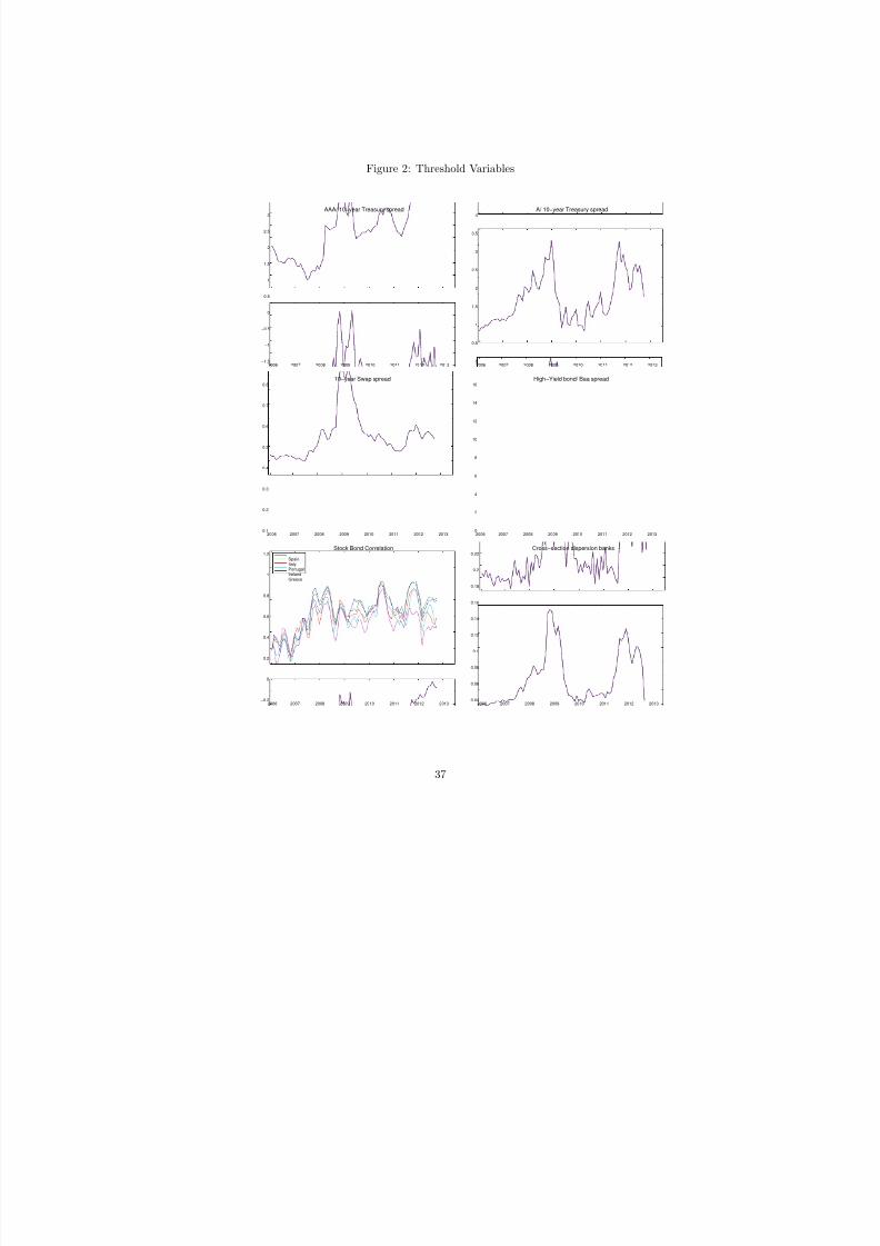
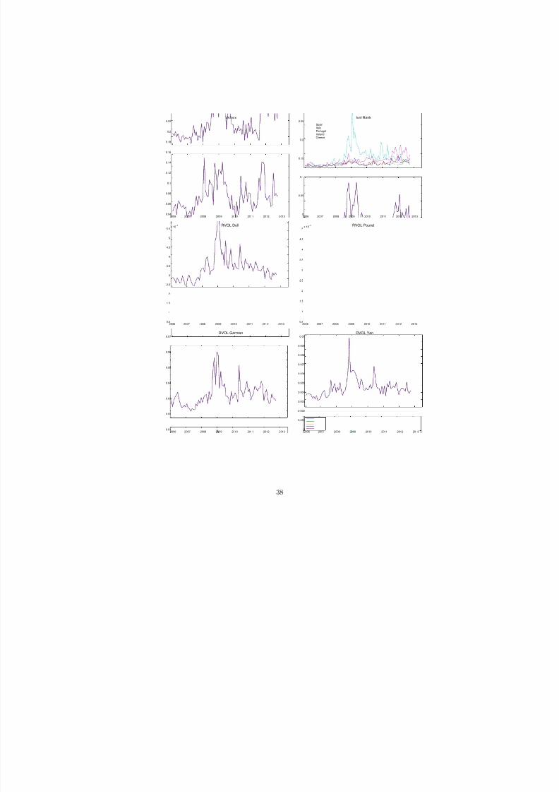
threshold variable. All threshold variables are plotted in Fig. 2.

1. Feedback loop from banks to sovereigns

• CDS prices are a reliable measure of risk as they are precisely the

premium an investor must pay to hedge the risk or express a credit

view of a reference entity. CDS indices are baskets of single CDS

covering specific sectors.15 Therefore the most straightforward

measure of financial risk is the price of CDS indices covering the

financial risk in the euro-area, SenFin and SubFin , both being in

the family of the i-Traxx Europe, a broad tradable credit default

swap family of indices .

Second, we construct disaggregate indicators of uncertainty and stress

in the banking sector borrowed from an aggregate indicator of systemic

risk designed by the Kansas Fed (Hakkio and Keeton, 2009). More

precisely, we compute components of their indicator with European

data:

by country, which makes the inclusion of the data composed of two observations irrelevant

in our panel estimates.15The main advantages of these new classes of credit derivatives are standardization and

liquidity, which explain their growth. CDS indices accounted for 43% of gross notional

amount of the CDS market in December 2012, up from 20% in 2004 (Vause, 2011). CDS

trading has continued to grow after 2007 (IOSCO, 2012). At the end of 2012, the gross

notional value of outstanding CDS contracts amounted to approximately 25 trillion US

dollars, and the corresponding net notional value to approximately 2.5 trillion US dollars.

The fact that the gross notional value of the CDS contracts has more than halved since

the peak of 2007 (with 60 trillion US dollars) is mostly attributed to the development of

compression mechanims that eliminate legally redundant contracts (Vause 2011).

12



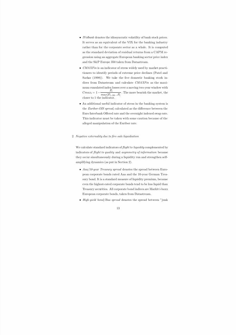
• IVolbank denotes the idiosyncratic volatility of bank stock prices.

It serves as an equivalent of the VIX for the banking industry

rather than for the corporate sector as a whole. It is computed

as the standard deviation of residual returns from a CAPM re-

gression using an aggregate European banking sector price index

and the S&P Europe 350 taken from Datastream.

• CMAXFin is an indicator of stress widely used by market practi-

tioners to identify periods of extreme price declines (Patel and

Sarkar (1998)). We take the five domestic banking stock in-

dices from Datastream and calculate CMAXFin as the maxi-mum cumulated index losses over a moving two-year window with

Cmaxt = 1 − P t

max[P t−24...P t]. The more bearish the market, the

closer to 1 the indicator.

• An additional useful indicator of stress in the banking system is

the Euribor-OIS spread , calculated as the difference between the

Euro Interbank Offered rate and the overnight indexed swap rate.

This indicator must be taken with some caution because of the

alleged manipulation of the Euribor rate.

2. Negative externality due to fire-sale liquidiation

We calculate standard indicators of flight to liquidity complemented by

indicators of flight to quality and asymmetry of information because

they occur simultaneously during a liquidity run and strengthen self-

amplifying dynamics (as put in Section 2).

• Aaa/10-year Treasury spread denotes the spread between Euro-

pean corporate bonds rated Aaa and the 10-year German Trea-

sury bond. It is a standard measure of liquidity premium, because

even the highest-rated corporate bonds tend to be less liquid than

Treasury securities. All corporate bond indices are Markit i-boxx

European corporate bonds, taken from Datastream.

• High-yield bond/Baa spread denotes the spread between ”junk

13



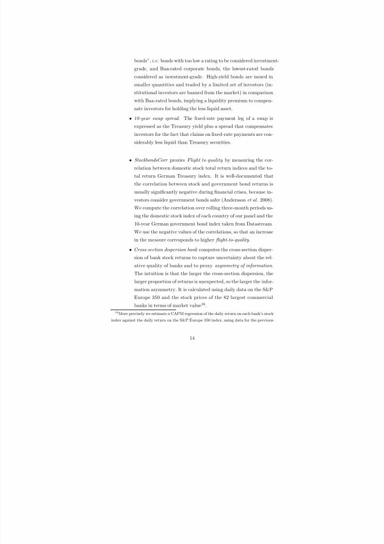
bonds”, i.e. bonds with too low a rating to be considered investment-

grade, and Baa-rated corporate bonds, the lowest-rated bonds

considered as investment-grade. High-yield bonds are issued in

smaller quantities and traded by a limited set of investors (in-

stitutional investors are banned from the market) in comparison

with Baa-rated bonds, implying a liquidity premium to compen-

sate investors for holding the less liquid asset.

• 10-year swap spread . The fixed-rate payment leg of a swap is

expressed as the Treasury yield plus a spread that compensates

investors for the fact that claims on fixed-rate payments are con-siderably less liquid than Treasury securities.

• StockbondsCorr proxies Flight to quality by measuring the cor-

relation between domestic stock total return indices and the to-

tal return German Treasury index. It is well-documented that

the correlation between stock and government bond returns is

usually significantly negative during financial crises, because in-

vestors consider government bonds safer (Andersson et al. 2008).We compute the correlation over rolling three-month periods us-

ing the domestic stock index of each country of our panel and the

10-year German government bond index taken from Datastream.

We use the negative values of the correlations, so that an increase

in the measure corresponds to higher flight-to-quality .

• Cross-section dispersion bank computes the cross-section disper-

sion of bank stock returns to capture uncertainty about the rel-

ative quality of banks and to proxy asymmetry of information .

The intuition is that the larger the cross-section dispersion, the

larger proportion of returns is unexpected, so the larger the infor-

mation asymmetry. It is calculated using daily data on the S&P

Europe 350 and the stock prices of the 82 largest commercial

banks in terms of market value16.

16More precisely we estimate a CAPM regression of the daily return on each bank’s stock

index against the daily return on the S&P Europe 350 index, using data for the previous

14



3. Control Variables

Last, we control for an overall effect of uncertainty and stress outside

the banking sector by including indicators on non-financial sectors:

• i-Traxx Europe comprises the most liquid 125 CDS referencing

European investment grade credits

• X-over comprises the most risky 40 constituents

• HiVol is a subset of the main Europe index consisting of what

are seen as the most risky 30 constituents

• Vstoxx is the European equivalent of the VIX, considered bymany to be the leading measure of market volatility17 .

• FTSE300 and S&P350 denote the returns of the European ag-

gregate stock market indices

• DomsticIndex is the matrix of the domestic stock returns in-

dices of the five countries in our panel (PSI, IBEX, ATHEX,

FTSEMIB, ISEQ).

• RvolGerm captures bond market volatility using the 10-year Ger-

man government bond index. It is the realized volatility com-

puted as the monthly average of absolute daily rate changes.

• Rvol Nonfi is the realized volatility of domestic non-financial sec-

tor stock market indices taken from Datastream.

• Rvoldoll , Rvolyen and Rvolpound are the realized volatility of

three bilateral euro exchange rates for the US dollar, the Japanese

yen and the British pound respectively.

Looking at the set of threshold variables plotted in Fig. 2, we see thatmost variables experienced a first peak during the subprime crisis, followed

12 months. The estimated coefficients are then used to calculate the forecast errors of the

current month. Last we calculate the interquartile range for these residuals in order to

keep the central 50%. The lower the interquartile value, the smaller the dispersion across

banks.17We use Vstoxx to proxy the European market volatility, while we use VIX to capture

international risk aversion.

15



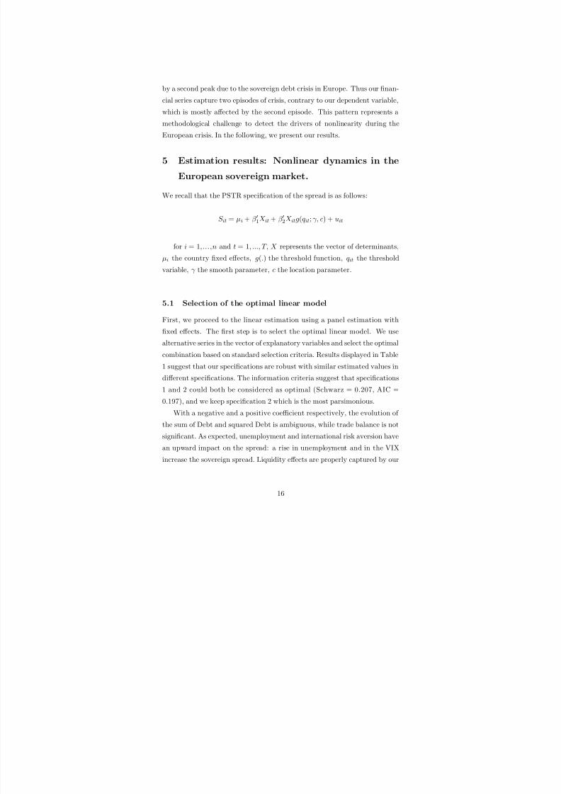
by a second peak due to the sovereign debt crisis in Europe. Thus our finan-

cial series capture two episodes of crisis, contrary to our dependent variable,

which is mostly affected by the second episode. This pattern represents a

methodological challenge to detect the drivers of nonlinearity during the

European crisis. In the following, we present our results.

5 Estimation results: Nonlinear dynamics in the

European sovereign market.

We recall that the PSTR specification of the spread is as follows:

S it = µi + β ′1X it + β ′2X itg(q it; γ, c) + uit

for i = 1,...,n and t = 1, ..., T, X represents the vector of determinants,

µi the country fixed effects, g(.) the threshold function, q it the threshold

variable, γ the smooth parameter, c the location parameter.

5.1 Selection of the optimal linear model

First, we proceed to the linear estimation using a panel estimation with

fixed effects. The first step is to select the optimal linear model. We use

alternative series in the vector of explanatory variables and select the optimal

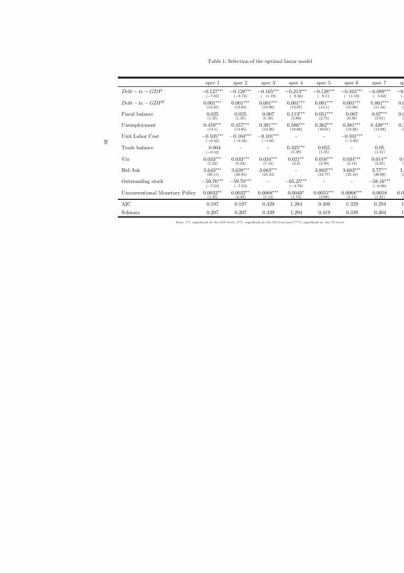
combination based on standard selection criteria. Results displayed in Table

1 suggest that our specifications are robust with similar estimated values in

different specifications. The information criteria suggest that specifications

1 and 2 could both be considered as optimal (Schwarz = 0.207, AIC =0.197), and we keep specification 2 which is the most parsimonious.

With a negative and a positive coefficient respectively, the evolution of

the sum of Debt and squared Debt is ambiguous, while trade balance is not

significant. As expected, unemployment and international risk aversion have

an upward impact on the spread: a rise in unemployment and in the VIX

increase the sovereign spread. Liquidity effects are properly captured by our

16



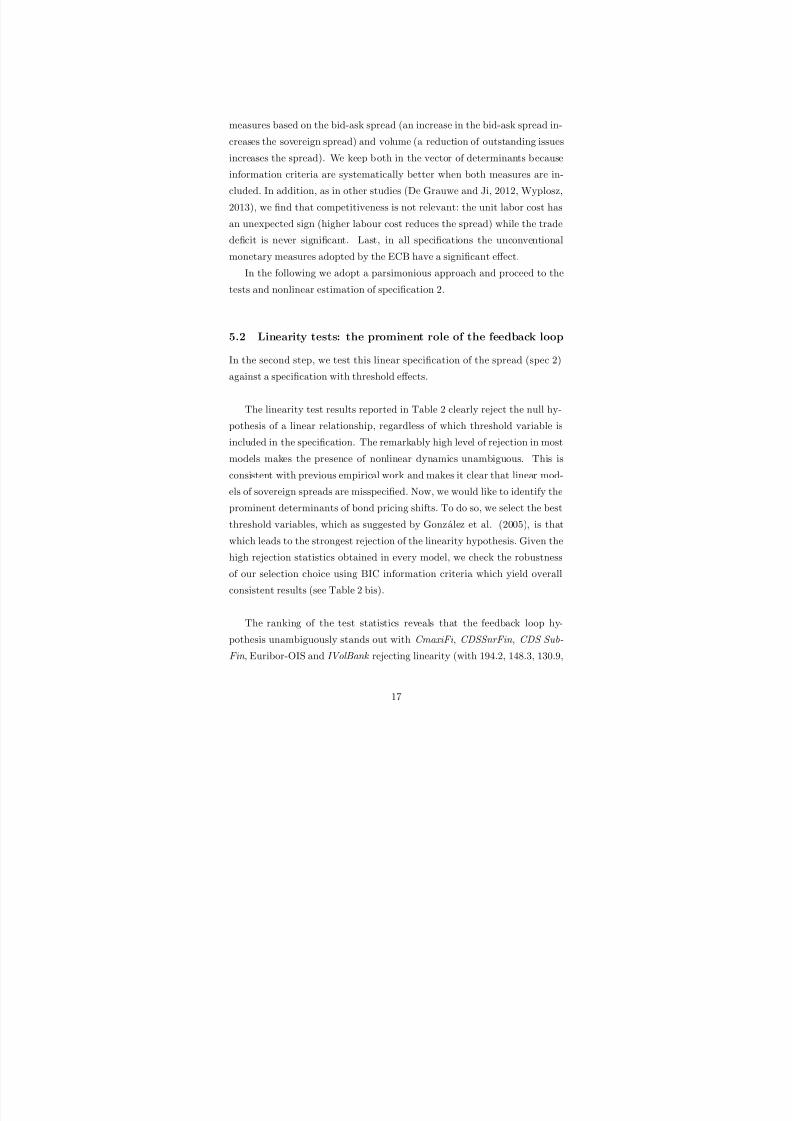
measures based on the bid-ask spread (an increase in the bid-ask spread in-

creases the sovereign spread) and volume (a reduction of outstanding issues

increases the spread). We keep both in the vector of determinants because

information criteria are systematically better when both measures are in-

cluded. In addition, as in other studies (De Grauwe and Ji, 2012, Wyplosz,

2013), we find that competitiveness is not relevant: the unit labor cost has

an unexpected sign (higher labour cost reduces the spread) while the trade

deficit is never significant. Last, in all specifications the unconventional

monetary measures adopted by the ECB have a significant effect.

In the following we adopt a parsimonious approach and proceed to thetests and nonlinear estimation of specification 2.

5.2 Linearity tests: the prominent role of the feedback loop

In the second step, we test this linear specification of the spread (spec 2)

against a specification with threshold effects.

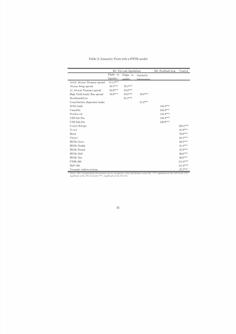
The linearity test results reported in Table 2 clearly reject the null hy-

pothesis of a linear relationship, regardless of which threshold variable is

included in the specification. The remarkably high level of rejection in most

models makes the presence of nonlinear dynamics unambiguous. This is

consistent with previous empirical work and makes it clear that linear mod-

els of sovereign spreads are misspecified. Now, we would like to identify the

prominent determinants of bond pricing shifts. To do so, we select the best

threshold variables, which as suggested by Gonzalez et al. (2005), is that

which leads to the strongest rejection of the linearity hypothesis. Given the

high rejection statistics obtained in every model, we check the robustness

of our selection choice using BIC information criteria which yield overall

consistent results (see Table 2 bis).

The ranking of the test statistics reveals that the feedback loop hy-

pothesis unambiguously stands out with CmaxiFi , CDSSnrFin , CDS Sub-

Fin , Euribor-OIS and IVolBank rejecting linearity (with 194.2, 148.3, 130.9,

17



119.4 and 116.2 respectively).18 It is interesting to observe that indicators

of uncertainty about the non -financial sector, rvol NonFin and rvol Germ ,

rank among the last with low statistics (39.5 and 30.4 resp.).

In sum, investors are sensitive to the risk in the banking sector, and

this triggers nonlinear dynamics. While the sovereign-nexus has been well-

documented before, we are the first to give a functional form to the subse-

quent amplification effects. More precisely, the pricing model is a nonlinear

function of fundamentals, where the weight of these fundamentals varies

with the risk of banks (we examine the evolution of the estimated coefficientbelow). The deterioration of market conditions for banks changes the way

investors price risk of the sovereigns.

Second, we can not reject the hypothesis of adverse effects due to fire-

sale liquidation, which also gets empirical support with LM statistics from

51.2 to 111.4. Flight to liquidity , Flight to quality and asymmetry of in-

formation have been unambiguously relevant factors of amplification in the

European sovereign debt crisis. Nevertheless, our empirical strategy ranks

the influence of both hypothesis and concludes that the sovereign-nexus was

prominent in driving non linearities.

Last the tests reveal that the volatility of different market segments play

a less significant role in nonlinear dynamics. While the volatility of FTSE

and S&P get a fairly high rejection statistics (111.8 and 111.6), other volatil-

ity measures such as Vstoxx do not confirm the effect of overall volatility

(LM= 64.2). This suggests that aggregate equity indices correlate with bank

stocks indices and thus convey a similar information. Volatility of the for-

eign exchange market is less relevant (rvol Pound , rvol Doll and rvol Yen get49.5, 40.0 and 43.9 resp) probably because intra-Euro zone, not extra-Euro

zone capital transfers have been relevant since 2010 (IMF, 2012a). Periph-

eral countries have suffered massive capital flight back to the core countries,

resulting in monetary fragmentation of the euro-zone. But the aggregate

external position of the eurozone has not deteriorated significantly.

18The BIC information criteria confirm the selection, see Table 2 bis

18



In the last step of our empirical investigation, we estimate the models

to compute the threshold values triggering regime switch and the variation

of coefficient loads.

5.3 Heteroegeneity in the sample

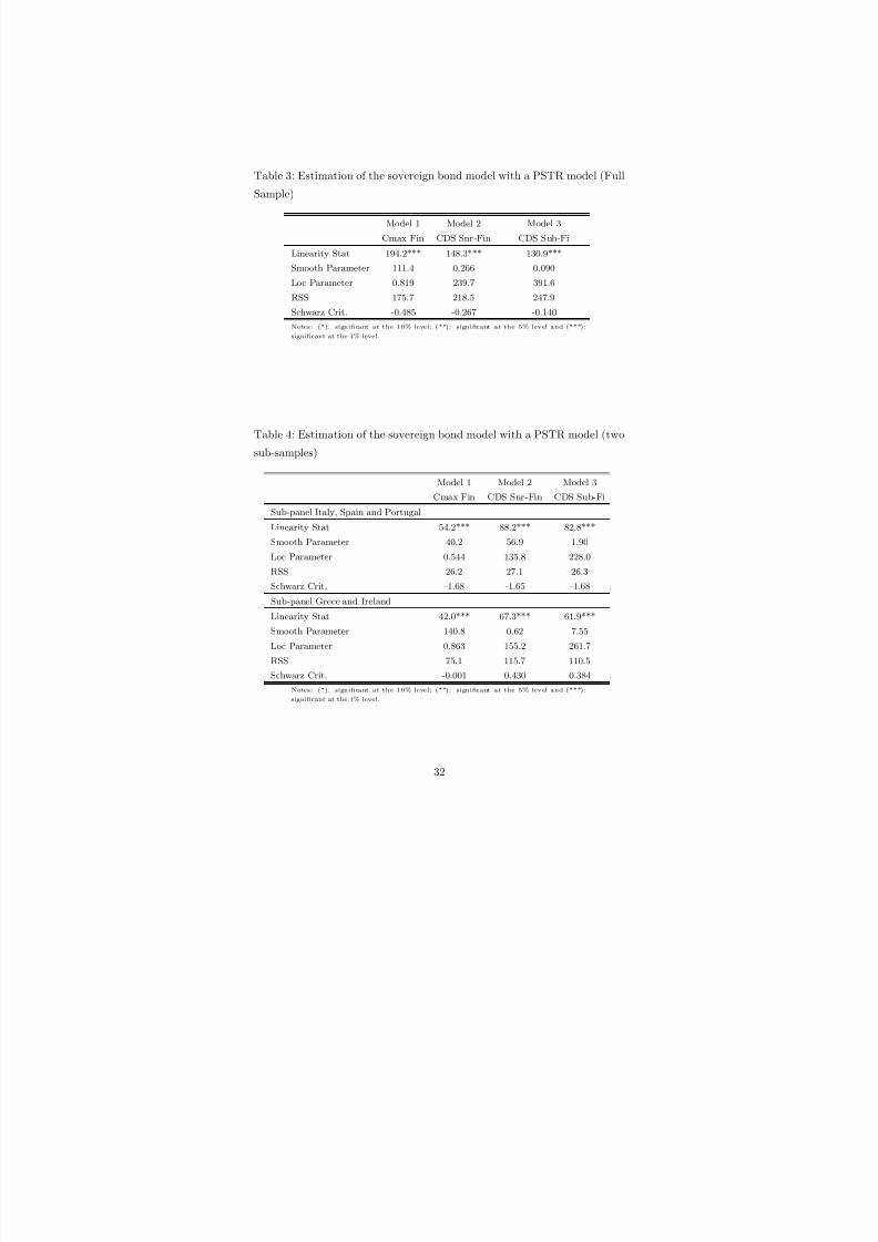
Table 3 reports the linearity test statistics, the smooth parameter, γ , the

location parameter c and the residual sum of squares in the three specifica-

tions that best reject linearity.

According to the selection criteria of Gonzalez et al. (2005), the in-

dicator of stress in the banking sector , CmaxFi is the optimal threshold

variable because it rejects linearity with the highest statistics. This is also

confirmed by the information criterion (Schwarz : -0.485In this specifica-

tion the smooth parameter is high (γ = 111.4), implying a sharp transition

between two extreme regimes. However, a thorough investigation indicates

that this variable CmaxFi captures the heterogeneity in our sample. In

fact, Italy, Spain and Portugal remain exclusively in the first regime (in

these countries CmaxiFi is always lower than the estimated location pa-

rameter c = 0.819 as shown in Fig 2, graph entitled max Financials), while

Ireland and Greece went from the first to the second regime (47 and 12

observations respectively as shown in Fig 2). Heterogeneity in the sample

is confirmed also in the specification including an individual threshold vari-

able, Ivol Bank , with similar patterns: the transition is sharp ( γ = 141.0),

and only Ireland and Greece went from the first to the second regime (27

and 12 observations respectively as shown in Fig 2, graph Ivol Bank ).

Therefore, while the five peripheral countries are usually gathered in the

same bundle, our estimates suggest that their spreads have a different dy-

namics. 19 This finding leads us to split our sample into two sub-samples,

one including Italy, Spain and Portugal, the other Greece and Ireland. The

19Gonzalez-Hermosillo and Johnson (2014) also point out heterogeneous dynamics in

the sovereign CDS of the five stressed countries.

19



smaller sub-sample still has 162 observations, which is sufficient for reason-

ably precise and stable estimates.

We re-estimate the model in each sub-sample (Table 4) and find that

linearity is strongly rejected again with a slightly different ranking from the

full sample.20 What is the threshold value and how do elasticities change?

To answer, we estimate β 1 and β 2 in Eq. (4) and we compare the determi-

nants coefficients before and after the transition, β 1 and β 1 + β 2 respectively.

We adopt a general-to-specific modeling approach where we eliminate non-

specific variables based on their statistical significance and the Schwartzinformation criterion.

5.3.1 Italy, Portugal and Spain

Results in Table 5 report the estimated coefficients in regime 1 and regime

2 (β 1 and β 1 + β 2). First, it indicates that the transition from the first to

the second regime is sharp (γ = 53.7) and the threshold value, c is 135.7 bp.

Our model predicts that investors price the sovereign risk differently when

the financial CDS index is over 135.7 bp. It is worth noting that this value

was crossed in autumn 2010 just after the Greek crisis broke. 21 Now we

examine the variation of the coefficient. Recall that amplification can be

modeled through increasing weights in the spread determination.

Our estimates suggest amplification effects that operate in regime 2

through a much stronger influence on the spread of all macroeconomic deter-

minants: debt, fiscal balance and unemployment as well as the international

risk aversion (| β ′1 + β ′2 |>| β ′1 |). In other words, when the price of iTraxx

CDS SnrFin exceeds 135.7 bp, the weight of these fundamentals increases

20In fact, in both samples, CDSSnrFin and CDS Sub-Fin best reject linearity (LM

=88.2/82.8 and 67.3/61.9 resp), while CmaxFi ranks lower. This result confirms that the

individual variable CmaxFi was mostly capturing heterogeneity in our previous estimates

(as was IvolBank ). In turn, CDS SnrFin and CDS Sub-Fin , which are two homogeneous

variables, account for the time-instability in the spread determination model.21In the alternative model γ = 2.18 which corresponds to a sharp transition too, see

Table 5.

20



in the determination model, so the shocks to fundamentals have more effect

on the bond spread. It is worth observing that the coefficients in the second

regime are much larger, often more than twice as much as in the first regime.

In sum, we detect sizable amplification effects.22 Last, we observe that the

influence of the SMP program has not changed during the crisis.

5.3.2 Greece and Ireland

Results of the second sub-sample including Greece and Ireland are reported

in Table 7. Transition is sharp and the threshold value is 155 bp, a valuesimilar to the previous sub-sample.23 However, the dynamics differ here

because amplification effects operate through a stronger influence of unem-

ployment only. In turn, the effects of debt and squared debt compensate

for each other, while the effects of the VIX and of the bid-ask spread are

positive, as expected, but they remain stable in the second regime. As in the

linear estimate, the unit labor cost has the same unexpected sign. An inter-

esting difference is that contrary to the previous sample, we observe that the

SMP has a negative effect on the spread in the second regime (β ′

1+ β ′

2 < 0).

In other words, our estimates suggest that the bond purchases carried out

by the ECB have counterbalanced amplification effects on the bond spreads

of Greece and Ireland.

22In turn, the influence of liquidity is ambiguous because the coefficients of both variables

capturing liquidity show two contrary movements in regime 2 : we find a stronger negative

influence of the relative stock of outstanding debt (implying that a deterioration of liquidity

affects the spread more in regime 2 than in regime 1), while the influence of the bid-ask

spread is lower in the second regime (| β ′1 + β ′2 |>| β ′1 |, implying that a rise in the bid-ask

spread affects the spread less in regime 2). In addition, we observe that the sign on unit

labor cost is contrary to the expected sign, as in the linear estimates (see Table 1). As

in the linear estimates, models excluding this variable have a lower RSS, so we decide to

keep it in the vector of explanatory variables.23The transition speed depends on γ and the distance between the threshold variable

and the threshold parameter c. Despite the low value of the slope parameter (γ = 0.43),

the fact that CDS indices increase strongly during the crisis implies that the transition

from one regime to the other is fairly fast, as in the other sub-sample.

21



Robustness

To check the robustness of our estimates, we proceed to alternative esti-

mates. In the first sub-sample (including Italy, Spain and Portugal), overall

amplification effects are confirmed when Cmax Fin is used as a thresh-

old variable in an alternative specification (see Table 6).24 Second, financial

CDS and sovereign bonds may price the same information, which would raise

an endogeneity bias due to simultaneity. To address this, we re-estimate our

optimal model by lagging the threshold variable. Linearity is rejected with a

similar statistic (LM = 63.2 versus 62 in the core estimate), and amplifica-

tion effects are confirmed. Last, we check that our nonlinearity finding does

not result from omitting the financial CDS index as an explanatory variable.

Our results are not affected by the introduction of the financial CDS index

in the vector of determinants (X it in Eq. 4), a result that confirms that this

variable nonlinearly affects the sovereign bond pricing.25

In the second sub-sample (including Greece and Ireland), we proceed

to the same alternative estimates reported in Table 8. Model 1 confirms

the stronger influence of debt and unemployment and indicates a strongerinfluence of liquidity, a result not uncovered in the core estimates. The

downward influence of the SMP is confirmed too.

6 Concluding remarks

We estimated the sovereign spread of five peripheral members of the euro-

area using panel non-linear estimation methods. Our objectives were three-

fold: 1) test for nonlinear sovereign bond pricing 2) discriminate betweentwo potential drivers of non-linearity, sovereign-bank nexus and liquidity

spirals and 3) quantify the threshold effects and coefficient regime shifts in

order to draw lessons for economic policy.

24We observe that the combined influence of debt and squared debt increases in regime

2 as well as the weight of fiscal balance and unemployment. Only the influence of VIX,

which is found to be stable, differs from the core estimate.25Results available on request.

22



Our PSTR estimations confirm that investors have priced the European

sovereigns differently since Fall 2010. The increasing risk in the banking

sector was not only a significant determinant of sovereign risk but it am-

plified the initial shock on fundamentals. A key indicator the ECB may

want to monitor to check the sovereign tensions is the premium of financial

i-Traxx CDS indices. The estimated thresholds to trigger the crisis regime

are quite low at less than 200 bp. We document amplification effects due

to liquidity spirals too, although to a lesser extent. In addition, while we

find unambiguously strong amplification dynamics in the sovereign bondsof Italy, Spain and Portugal, we find lower effect in Greece and Ireland.

It suggest that the latter are mostly facing domestic issues while the three

other peripherals are highly vulnerable to a shock at the aggregate Euro-

pean level. In these three countries, the elasticity of sovereign yield to a

variation of most fundamental more than doubles in the crisis regime. Why

should we care? Because it suggests that addressing domestic fiscal imbal-

ances and real economy issues will lower down sovereign tensions only when

the aggregate banking-sovereign nexus is definitely cleaned out. Doubts un-

fortunately persist about the ability of the modest banking union recently

adopted to restore banking stability.

References

1. Acharya, V., and Steffen, S. ”The greatest carry trade ever? Under-

standing Eurozone bank risks”, CEPR Discussion Paper 9432 (2013).

2. Acharya, V., Drechsler, I., and Schnabl, P. ”A Pyrrhic victory? Bank

bailouts and sovereign credit risk”, Journal of Finance, forthcoming.

3. Adrian, T., and Shin, H. S. ”The Changing Nature of Financial Inter-

mediation and the Financial Crisis of 2007-2009”. Annual Review of

Economics , 2(1), 603-618 (2010).

4. Afonso A., P. Gomes and P. Rother, “What “hides” behind sovereign

debt ratings?”, European Central Bank Working Paper, 711 (2007).

23



5. Aizenman J, M. M. Hutchison and Y. Jinjarak, ”What is the risk

of European sovereign debt default? Fiscal space, CDS spread, and

market pricing of risk”, NBER WP 17407 (2011).

6. Allen, W. A. and Moessner, R. ”The liquidity consequences of the euro

area sovereign debt crisis”. BIS Working Paper (2013).

7. Andersson, M. Krylova, E. and Vahamaa, S. ”Why Does the Corre-

lation between Stock and Bond Returns Vary over Time?”, Applied

Financial Economics , 18(2) (2008).

8. Arghyrou, M. G. and Kontonikas, A., ”The EMU sovereign-debt cri-

sis: Fundamentals, expectations and contagion,” European Economy

- Economic Papers 436 , Directorate General Economic and Monetary

Affairs, European Commission (2011).

9. Attinasi, M. G., Checherita, C. and Nickel, C., ”What explains the

surge in euro area sovereign spreads during the financial crisis of 2007-

09?”, ECB Working Paper (2009).

10. Baba, N., and Inada, M., ”Price discovery of subordinated creditspreads for Japanese mega-banks: Evidence from bond and credit

default swap markets”. Journal of International Financial Markets,

Institutions and Money , 19(4), 616-632 (2009).

11. Bernanke, B., Gertler, M. and Gilchrist, S. ”The financial accelerator

in a quantitative business cycle framework.” Handbook of macroeco-

nomics 1 1341-1393, (1999).

12. Blanco, R., Brennan, S. and Marsh, I. W., ”An Empirical Analysis of

the Dynamic Relation between Investment-Grade Bonds and Credit

Default Swaps”. Journal of Finance , 60, 2255-2281 (2005).

13. Borgy, V., Laubach, T., Mesonnier J.-S. and Renne, J.-P., “Fiscal

Sustainability, Default Risk and Euro Area Sovereign Bond Spreads

Markets”, Document de travail n.350, Banque de France (2011).

24



14. Brock, W. A., Hommes, C. H. and Wagner, F. O. O. ”More hedging

instruments may destabilise markets.” J. Econ. Dynam. Cont. 33,

1912-1928 (2009).

15. Brunnermeier, M., Crockett, A., Goodhart C., Persaud, A., Shin, H.,

The Fundamental Principles of Financial Regulation , ICMB-CEPR

Geneva Reports on the World Economy series (2009).

16. Brunnermeier, M. Oehmke, M., ”Complexity in financial markets”,

Technical report, Princeton Working Paper 2009/2, 4 (2009).

17. Brunnermeier, M. Pedersen, L.H., ”Market liquidity and funding liq-

uidity”, Review of Financial Studies , 22, 2201-2238 (2009).

18. Cantor, R. Packer, F., ”Determinants and impact of sovereign credit

ratings”, FRB NYEconomic Policy Review , 2(2) (1996).

19. Coimbra, N., ”Sovereigns at risk: a dynamic model of sovereign debt

and banking leverage”, London Business School (January 2014).

20. Davies R.B. ”Hypothesis testing when a nuisance parameter is present

only under the alternative”, Biometrika 74, 33-43 (1987).

21. De Grauwe, P., Y. Ji, ” Self-fulfilling crises in the Eurozone: an em-

pirical test”, Journal of international money and finance , 34, 15-36

(2013).

22. De Grauwe, P.,”A fragile eurozone in search of a better governance”,

CESIFO Working Paper , n.3456 (2011).

23. De Grauwe, P., ”The financial crisis and the future of the eurozone”,

Bruges European Economic Policy Briefings , 21 (2010).

24. Delatte, AL., Gex, M. and A. Lopez-Villavicencio, ”Has the CDS mar-

ket influenced the borrowing cost of European countries during the

sovereign crisis?”, Journal of International Money and Finance , 31(3)

(2012).

25. Duffie, D. and Singleton, K., ”Modeling term structures of defaultable

bonds”, Review of Financial Studies , 12(4), 687-720 (1999).

25



26. Dunne, P., Moore, M. and Portes, R. ”Benchmark Status in Fixed

Income Asset Markets.” Journal of Business Finance and Accounting

34.9-10 1615-1634 (2007).

27. Edwards, S. ”The pricing of bonds and bank loans in international

markets: An empirical analysis of developing countries’ foreign bor-

rowing”, European Economic Review , 30 (3), 565-589 (1986).

28. Eichengreen, B. Portes, R., ”After the Deluge: Default, Negotiation

and Readjustment in the Interwar Years”, in B. Eichengreen and P.

Lindert (eds.), The International Debt Crisis in Historical Perspective , pp. 12-47(MIT Press, 1989).

29. Favero, C., Pagano, M. and von Thadden, E.L. ”How Does Liquidity

Affect Government Bond Yields?”, Journal of Financial and Quanti-

tative Analysis , 45, 107-134 (2010).

30. Favero, C. and A. Missale, “”Sovereign Spreads in the Euro Area.

Which Prospects for a Eurobond?” Economic Policy , 27(70), 231-273

(2012).

31. Fouquau J., Hurlin C., Rabaud I., ”The Feldstein-Horioka Puzzle: a

Panel Smooth Transition Regression Approach.” Economic Modelling ,

20, 284-299 (2008).

32. Geanakoplos, J. and Polemarchakis, H. ”Existence, regularity and con-

strained suboptimality of competitive allocations when markets are

incomplete”, in W. Heller, R. Starr and D. Starrett (eds), Essays in

Honor of K. Arrow , Cambridge: Cambridge University Press (1986).

33. Geanakoplos, J. ”The leverage cycle.” NBER Macroeconomics Annual

2009 , Volume 24. University of Chicago Press. 1-65 (2010).

34. Gennaioli, N., Martin, A. and Rossi, S., ”Sovereign default, domestic

banks and financial institutions”, CEPR Discussion Paper 7955 (2010).

35. Gerlach, S., A. Schulz and G.B. Wolff, ”Banking and sovereign risk

in the euro area”, Deutsche Bundesbank Discussion Paper n.09/2010

(2010).

26



36. Geyer, A. Kossmeier, S and Pichler, S., ”Measuring systematic risk in

EMU government yield spreads”, Review of Finance , 8(2), (171-197)

(2004).

37. Gonzalez A., Terasvirta T. and D. van Dijk ”Panel smooth transition

regression models”, SEE/EFI Working Paper Series in Economics and

Finance No. 604 (2005).

38. Gorton, G. and Metrick, A., ”Securitized banking and the run on

repo”, Journal of Financial Economics , 104(3), 425-451 (2012)

39. Hamilton J.D., Time series analysis , Princeton University Press (1994).

40. Hakkio C.S and Keeton, W., ”Financial Stress: What is it? How can

it be measured?”, Federal Reserve Bank of Kansas City, Economic

Review (2009).

41. Haugh, D., P. Ollivaud and D. Turner, “What Drives Sovereign Risk

Premiums?: An Analysis of Recent Evidence from the Euro Area”,

OECD Economics Department Working Papers, No. 718, OECD Pub-

lishing (2009).

42. Hollo, D. Kremer, M. and Lo Duca, M., ”CISS-a composite indicator

of systemic stress in the financial system”, ECB Working Paper (2012).

43. Huizinga, H., and Demirguc-Kunt, A., ”Are banks too big to fail or

too big to save? International evidence from equity prices and CDS

spreads”, European Banking Center Discussion Paper 2010-15 (2010).

44. IMF, ”World Economic Outlook. Coping with High Debt and Slug-

gish Growth”, World Economic and Financial Surveys, InternationalMonetary Fund, Washington (2012a).

45. IMF, ”Global Financial Stability Report. The Quest for Lasting Sta-

bility”, World Economic and Financial Surveys, International Mone-

tary Fund, Washington (2012b).

46. IOSCO, ”The credit default swap”, Technical Report, International

Organization of Securities Commissions (2012)

27



47. Lane, P. (2012) ”The European sovereign debt crisis”, Journal of

Economic Perspectives , 26(3) (2012).

48. Longstaff, F.A and Schwartz, E.S, ”A simple approach to valuing

risky fixed and floating rate debt”, Journal of Finance , 50(3), 789-

819 (1995).

49. Longstaff, F.A, Pan Jun, Pedersen, L.H. and Singleton K.J. , ”How

Sovereign Is Sovereign Credit Risk?,” American Economic Journal:

Macroeconomics, American Economic Association, vol. 3(2), pages

75-103 (2011).

50. Montfort A. and J.P. Renne, “Credit and liquidity risks in euro-area

sovereign yield curves”, Document de travail n.352 Banque de France

(2011).

51. Palladini, G, and R Portes, “Sovereign CDS and Bond Price Dynamics

in the Eurozone”, CEPR Discussion Paper 8651 (2011).

52. Paris P., and Wyplosz C. , ”To end the Eurozone crisis, bury the debt

forever”, voxEU, 6 August (2013).

53. Patel, S. and A. Sarkar, ”Stock Market Crises in Developed and Emerg-

ing Markets”, Financial Analysts Journal , 54(6) 50-59 (1998).

54. Rey, H., ”Dilemma not Trilemma: The global financial cycle and

monetary policy independence.” Jackson Hole Economic Symposium.

(2013).

55. Simsek, A., ”Speculation and Risk Sharing with New Financial As-

sets”, The Quarterly Journal of Economics , 128 (3): 1365-1396 (2013).

56. Stiglitz, J., ”The Inefficiency of the Stock Market Equilibrium”, Re-

view of Economic Studies , 49(2), 241-261 (1982)

57. Tavakoli, J., Structured finance and collateralized debt obligations: new

developments in cash and synthetic securitization , Wiley (2008).

58. Vause, N., ”Enhanced BIS statistics on credit risk transfer”, BIS Quar-

terly Review , December (2011).

28



59. Wyplosz, C. ”Eurozone Crisis: It’s About Demand, not Competitive-

ness.” The Graduate Institute, Geneva (2013).

29



Table 1: Selection of the optimal linear model

spec 1 spec 2 spec 3 spec 4 spec 5

Debt − to − GDP −0.127∗∗∗(−7.83)

−0.128∗∗∗(−8.73)

−0.165∗∗∗(−11.19)

−0.213∗∗∗(−8.56)

−0.128∗∗∗(−8.11)

−

Debt − to − GDP 2 0.001∗∗∗(13.35)

0.001∗∗∗(13.62)

0.001∗∗∗(15.96)

0.001∗∗∗(12.07)

0.001∗∗∗(14.1)

0

Fiscal balance 0.025(1.35)

0.025(1.35)

0.007(0.38)

0.113∗∗∗(3.88)

0.051∗∗∗(2.73)

Unemployment 0.459∗∗∗(14.1)

0.457∗∗∗(14.85)

0.381∗∗∗(12.26)

0.586∗∗∗(10.66)

0.362∗∗∗(10.61)

0

Unit Labor Cost −0.105∗∗∗

(−6.42)

−0.104∗∗∗

(−6.56)

−0.101∗∗∗

(−5.95)

- - −

Trade balance −0.004(−0.10)

- - 0.325∗∗∗(5.38)

0.055(1.35)

Vix 0.033∗∗∗(5.22)

0.033∗∗∗(5.24)

0.034∗∗∗(5.14)

0.021∗∗(2.2)

0.016∗∗∗(2.56)

0

Bid-Ask 3.643∗∗∗(26.11)

3.639∗∗∗(26.83)

3.683∗∗∗(25.44)

- 3.803∗∗∗(24.77)

3

Outstanding stock −59.76∗∗∗(−7.53)

−59.70∗∗∗(−7.53)

− −65.25∗∗∗(−4.78)

-

Unconventional Monetary Policy 0.0032∗∗(2.35)

0.0032∗∗(2.38)

0.0068∗∗∗(5.14)

0.0040∗(1.73)

0.0055∗∗∗(3.98)

0

AIC 0.197 0.197 0.329 1.284 0.409

Schwarz 0.207 0.207 0.339 1.294 0.419

Note: (*): significant at the 10% level; (**): significant at the 5% level and (***): significant at the 1% level.

3 0



Table 2: Linearity Tests wth a PSTR model

H1: Fire-sale liquidation H2: Feedback loop Control

Flight to

liquidity

Flight to

quality

Asymetry

information

AAA/ 10-year Treasury spread 111.4***10-year Swap spread 78.2*** 78.2***

A/ 10-year Treasury spread 84.8*** 84.8***

High-Yield bond/ Baa spread 70.8*** 70.8*** 70.8***

StockbondsCorr 91.4***

Cross-Section dispersion banks 51.2***

IVOL bank 116.2***

CmaxFin 194.2***

Euribor-ois 119.4***

CDS Snr-Fin 148.3***

CDS Sub-Fin 130.9***

I-traxx Europe 108.4***

X-over 91.9***

Hivol 79.0***

Vstoxx 64.2***

RVOL Germ 29,5***

RVOL Nonfin 41,4***

RVOL Pound 47,9***

RVOL Doll 36,6***

RVOL Yen 39.6***

FTSE 300 111.8***

S&P 350 111.6***

Domestic indices returns 37.7***

Notes: The corresponding LM statistic has an asymptotic χ2(p) distribution under H 0. (*): significant at the 10% level; (**):

significant at the 5% level and (***): significant at the 1% level.

31



Table 3: Estimation of the sovereign bond model with a PSTR model (Full

Sample)

Model 1 Model 2 Model 3

Cmax Fin CDS Snr-Fin CDS Sub-Fi

Linearity Stat 194.2*** 148.3*** 130.9***

Smooth Parameter 111.4 0.266 0.090

Loc Parameter 0.819 239.7 391.6

RSS 175.7 218.5 247.9

Schwarz Crit. -0.485 -0.267 -0.140

Notes: (*): significant at the 10% level; (**): significant at the 5% level and (***):

significant at the 1% level.

Table 4: Estimation of the sovereign bond model with a PSTR model (two

sub-samples)


Cmax Fin CDS Snr-Fin CDS Sub-Fi

Sub-panel Italy, Spain and Portugal

Linearity Stat 54.2*** 88.2*** 82.8***


Loc Parameter 0.544 135.8 228.0

RSS 26.2 27.1 26.3

Schwarz Crit. -1.68 -1.65 -1.68

Sub-panel Grece and Ireland

Linearity Stat 42.0*** 67.3*** 61.9***


Loc Parameter 0.863 155.2 261.7

RSS 75.1 115.7 110.5

Schwarz Crit. -0.001 0.430 0.384

Notes: (*): significant at the 10% level; (**): significant at the 5% level and (***):

significant at the 1% level.

32



Table 5: Estimates of the sovereign bond model with a PSTR model for

Italy, Spain & Portugal


CDS Snr Fin CDS Sub Fin CMax Fi

β 1 β 2 β 1 β 2 β 1 β 2

Debt 0.0212∗∗∗(3.54)

0.035∗∗∗(4.28)

0.011∗(1.94)

0.042∗∗∗(5.23)

0.129∗∗∗(5.91)

−0.031∗∗∗(−3.48)

Squared Debt - - - - −0.0004∗∗∗(−3.45)

0.0002∗∗∗(3.48)

Fiscal Balance 0.004(0.30)

0.154∗∗(2.40)

0.053∗∗∗(3.43)

0.137∗∗(2.12)

−0.053∗(−1.80)

0.170∗∗∗(3.90)

Unemployment 0.015(0.54)

0.112∗∗∗(2.70)

0.100∗∗∗(3.50)

0.116∗∗∗(2.65)

−0.155∗∗∗(−3.04)

0.179∗∗∗(4.62)

Unit Labor Cost 0.004(0.48)

−0.024∗∗(−2.54)

−0.006(−0.66)

−0.028∗∗∗(−2.89)

- -

VIX 0.015∗∗∗

(5.67)

0.035∗∗∗

(4.71)

0.014∗∗∗

(4.9)

0.038∗∗∗

(5.27)

0.021∗∗∗

(5.99)

0.002(0.25)

Bid-Ask 15.18∗∗∗(12.9)

−10.44∗∗∗(−8.14)

43.05∗∗∗(6.16)

−38.33∗∗∗(−5.49)

7.71∗∗∗(10.66)

−2.51∗∗∗(−3.86)

Outstanding Stock of gov −4.61(−0.78)

−9.32∗∗∗(−5.70)

−11.67∗∗(−1.99)

−9.61∗∗∗(−6.57)

- -

Unconv. Monet. Policy 0.0074∗∗∗(4.20)

0.0013(0.57)

0.0072∗∗∗(5.79)

0.0003(−0.15)

0.0071∗∗∗(7.34)

0.0019(1.38)

Smooth Parameter γ 60.3 2.18 39.62

Loc Parameter c 135.7 227.9 0.545

Linearity Stat. 96.9∗∗∗ 90.0∗∗∗ 62.0∗∗∗

RSS 27.6 26.81 26.4

Schwarz Crit. -1.685 -1.716 -1.786

Notes: The T-stat in parentheses are corrected for heteroskedasticity. (*): significant at the 10% level; (**): significant at

the 5% level and (***): significant at the 1% level.β1 and β2 correspond to the coefficient in Eq (11). β1 is the coefficientin the first extreme regime . The coefficient in the second extreme regime is β1 + β2.

33



Table 6: Estimates of the sovereign bond model with a PSTR model for

Greece & Ireland


CDS Snr Fin CDS Sub Fin Cmax Fi

β 1 β 2 β 1 β 2 β 1 β 2

Debt −0.101∗∗∗(−4.20)

0.086∗∗(2.13)

−0.114∗∗∗(−4.99)

0.067(1.53)

−0.296∗∗∗(−9.28)

0.242∗∗∗(4.05)

Squared Debt 0.0005∗∗∗(4.89)

−0.0004∗(−1.82)

0.001∗∗∗(6.50)

0.000(−1.49)

0.001∗∗∗(10.89)

0.000(−0.48)

Fiscal Balance 0.057∗∗∗(2.63)

0.031(0.65)

0.056∗∗∗(2.91)

−0.047(−0.81)

−0.092∗∗∗(−2.61)

0.109∗∗(2.28)

Unemployment 0.57∗∗∗(8.98)

0.69∗∗∗(4.30)

0.602∗∗∗(9.48)

0.639∗∗∗(3.99)

0.849∗∗∗(7.85)

0.020(0.10)

Unit Labor Cost 0.03∗(1.73)

−0.008∗∗∗(−4.13)

0.022(1.45)

−0.082∗∗∗(−4.02)

−0.036∗∗(−2.05)

−0.048∗∗(−2.10)

VIX 0.03∗∗∗

(3.84)

−0.0135(−0.44)

0.033∗∗∗

(4.53)

−0.007(−0.23)

0.025∗∗∗

(3.99)

0.019(0.83)

Bid-Ask 4.55∗∗∗(3.5)

−1.7(−1.27)

4.735∗∗∗(4.19)

−1.904(−1.61)

2.67∗∗∗(6.97)

1.175∗∗(2.05)

Outstanding Stock of gov - - - - 161.9 ∗ ∗∗(3.31)

−632.3∗∗∗(−5.96)

Uncon. Monet. Policy 0.026∗∗∗(6.26)

−0.038∗∗∗(−5.48)

0.024∗∗∗(6.49)

−0.033∗∗∗(−4.49)

0.0275∗∗∗(7.20)

−0.0459∗∗∗(−7.20)

Smooth Parameter γ 0.43 6.57 140.8

Loc Parameter c 154.8 262.0 0.863

Linearity Stat. 63.4*** 60.2*** 42.0***

RSS 116.3 111.1 75.1

Schwarz Crit. 0.358 0.312 -0.001

Notes: The T-stat in parentheses are corrected for heteroskedasticity. (*): significant at the 10% level; (**): significant at

the 5% level and (***): significant at the 1% level.β1 and β2 correspond to the coefficient in Eq (11). β1 is the coefficient

in the first extreme regime . The coefficient in the second extreme regime is β1 + β2.

34



Figure 1: Dependent and Explanatory Variables

2006 2007 2008 2009 2010 2011 2012 2013−5

0

5

10

15

20

25

30 Sovereign Spread

SpainItalyPortugalIrelandGreece

2006 2007 2008 2009 2010 2011 2012 201320

40

60

80

100

120

140

160

180 Debt to GDP


2006 2007 2008 2009 2010 2011 2012 20130

0.5

1

1.5

2

2.5

3

3.5x 10

4 Squared value of Debt to GDP


2006 2007 2008 2009 2010 2011 2012 2013−35

−30

−25

−20

−15

−10

−5

0

5

Fiscal Deficit

SpainItaly

Portugal

Ireland

Greece

2006 2007 2008 2009 2010 2011 2012 201395

100

105

110

115

120

125

Unit Labor Cost


35



2006 2007 2008 2009 2010 2011 2012 2013−20

−15

−10

−5

0

5

10

15

20

25

30

Trade Balance

SpainItaly

PortugalIreland

Greece

2006 2007 2008 2009 2010 2011 2012 20130

5

10

15

20

25

30

Unemployment Rate

SpainItaly

PortugalIreland

Greece

2006 2007 2008 2009 2010 2011 2012 20130

1

2

3

4

5

6 Bid ASk Spread


2006 2007 2008 2009 2010 2011 2012 20130

0.05

0.1

0.15

0.2

0.25

0.3

0.35

Securities Issued

Spain

Italy

Portugal

Ireland

Greece

2006 2007 2008 2009 2010 2011 2012 201310

20

30

40

50

60

70

CBOE Volatility Index

2006 2007 2008 2009 2010 2011 2012 20130

0.5

1

1.5

2

2.5

3x 10

5 Securities Markets Programme

36



Figure 2: Threshold Variables

2006 2007 2008 2009 2010 2011 2012 2013−1.5

−1

−0.5

0

0.5

1

1.5

2

2.5

3

AAA/ 10−year Treasury spread

2006 2007 2008 2009 2010 2011 2012 20130

0.5

1

1.5

2

2.5

3

3.5

4

A/ 10−year Treasury spread

2006 2007 2008 2009 2010 2011 2012 20130.1

0.2

0.3

0.4

0.5

0.6

0.7

0.8

10−year Swap spread

2006 2007 2008 2009 2010 2011 2012 20130

2

4

6

8

10

12

14

16

High−Yield bond/ Baa spread

2006 2007 2008 2009 2010 2011 2012 2013−0.2

0

0.2

0.4

0.6

0.8

1

1.2

Stock Bond Correlation


2006 2007 2008 2009 2010 2011 2012 20130.04

0.06

0.08

0.1

0.12

0.14

0.16

0.18

0.2

0.22

Cross−section dispersion banks

37



2006 2007 2008 2009 2010 2011 2012 20130.04

0.06

0.08

0.1

0.12

0.14

0.16

0.18

0.2

0.22

Vstoxx

2006 2007 2008 2009 2010 2011 2012 20130

0.05

0.1

0.15

0.2

0.25

Ivol Bank


2006 2007 2008 2009 2010 2011 2012 20130.5

1

1.5

2

2.5

3

3.5

4

4.5

5

5.5x 10

−3 RVOL Doll

2006 2007 2008 2009 2010 2011 2012 20130.5

1

1.5

2

2.5

3

3.5

4

4.5

5x 10

−3 RVOL Pound

2006 2007 2008 2009 2010 2011 2012 20130.01

0.02

0.03

0.04

0.05

0.06

0.07

RVOL German

2006 2007 2008 2009 2010 2011 2012 20130

0.001

0.002

0.003

0.004

0.005

0.006

0.007

0.008

0.009

0.01

RVOL Yen

38



2006 2007 2008 2009 2010 2011 2012 20130

0.002

0.004

0.006

0.008

0.01

0.012

0.014

0.016

0.018

Rvol Non Financial


2006 2007 2008 2009 2010 2011 2012 20130

0.1

0.2

0.3

0.4

0.5

0.6

0.7

0.8

0.9

1

Cmax Financials

Spain

Italy

Portugal

Ireland

Greece

Loc Parameter

2006 2007 2008 2009 2010 2011 2012 2013700

800

900

1000

1100

1200

1300

1400

1500

1600

FTSE 300

2006 2007 2008 2009 2010 2011 2012 2013700

800

900

1000

1100

1200

1300

1400

1500

1600

1700

SPE 350

2006 2007 2008 2009 2010 2011 2012 2013−0.15

−0.1

−0.05

0

0.05

0.1

Domestic Stock Returns

Spain

Italy

Portugal

Ireland

Greece

2006 2007 2008 2009 2010 2011 2012 201320

40

60

80

100

120

140

160

180

200

i−traxx Europe

39



2006 2007 2008 2009 2010 2011 2012 2013100

200

300

400

500

600

700

800

900

1000

1100

X−over

2006 2007 2008 2009 2010 2011 2012 20130

50

100

150

200

250

300

350

400

450

500

HiVol

2006 2007 2008 2009 2010 2011 2012 20130

100

200

300

400

500

600CDS Sub Fin

2006 2007 2008 2009 2010 2011 2012 20130

50

100

150

200

250

300

CDS SnrFin

40



Figure 3: I-Traxx CDS Indices, Volume and Prices

120

160

200

240

280

4,000,000,000

5,000,000,000

6,000,000,000

7,000,000,000

8,000,000,000

III IV I II III IV I II III

2010 2011 2012

Price SeniorFin CDSVolume SeniorFin CDS

200

300

400

500

600

400,000,000

800,000,000

1,200,000,000

1,600,000,000

2,000,000,000

2,400,000,000


2010 2011 2012

Price SubFin CDSVolume SubFin CDS

80

100

120

140

160

180

200

2.0E+10

2.4E+10

2.8E+10

3.2E+10

3.6E+10

4.0E+10


2010 2011 2012

Price Itraxx EuropeVolume Itraxx Europe

Notes: Source: DTCC. Lh scale : prices in basis points. Rh scale: volumes in

US$

Regime Dependent risk threshold

Documents

Transcript of Regime Dependent risk threshold