References - link.springer.com3A978-0-387-29930-3%2F1… · R. V. Churchill, 1972. Operational...

A. References 255

AReferences

1. S. Axler, 1997. Linear Algebra Done Right, 2nd ed., Springer-Verlag, NewYork. (A good second course in linear algebra.)

2. F. Brauer & C. Castillo-Chavez, 2001. Mathematical Models in PopulationBiology and Epidemiology, Springer-Verlag, New York. (Concentrates onpopulations, disease dynamics, and resource management, for advancedundergraduates.)

3. N. Britton, 2003. Essential Mathematical Biology, Springer-Verlag, NewYork. (An introduction to mathematical biology with broad coverage.)

4. S. C. Chapra, 2005. Applied Numerical Methods with MATLAB for Engi-neers and Scientists, McGraw-Hill, Boston. (A blend of elementary numer-ical analysis with MATLAB instruction.)

5. R. V. Churchill, 1972. Operational Mathematics, 3rd ed., McGraw-Hill,New York. (This classic book contains many applications and an extensivetable of transforms.)

6. F. Diacu, 2000. An Introduction to Differential Equations, W. H. Freeman,New York. (An elementary text with a full discussion of MATLAB, Maple,and Mathematica commands for solving problems in differential equations.)

7. C. H. Edwards & D. E. Penney, 2004. Applications Manual: DifferentialEquations and Boundary Value Problems, 3rd ed., Pearson Education, Up-per Saddle River, NJ. (A manual with a detailed discussion and illustrationof MATLAB, Maple, and Mathematica techniques.)

256 A. References

8. D. J. Higham & N. J. Higham, 2005. MATLAB Guide, 2nd ed., SIAM,Philadelphia. (An excellent source for MATLAB applications.).

9. M. W. Hirsch, S. Smale, & R. L. Devaney, 2004. Differential Equations,Dynamical Systems, & An Introduction to Chaos, Elsevier, New York. (Areadable, intermediate text with an excellent format.)

10. D. Hughes-Hallet, et al. 2005. Calculus: Single Variable, 4th ed, John Wiley,New York. (Chapter 11 of this widely used calculus text is an excellentintroduction to simple ideas in differential equations.)

11. W. Kelley & A. Peterson, 2003. The Theory of Differential Equations, Pear-son Education, Upper Saddle River NJ. (An intermediate level text focuseson the theory of differential equations.)

12. J. H. Kwak & S. Hong, 2004. Linear Algebra, 2nd ed., Birkhauser, Boston.(A readable and thorough introduction to matrices and linear algebra.)

13. G. Ledder, 2005. Differential Equations: A Modeling Approach, McGraw-Hill, New York. (An introductory text that contains many interesting mod-els and projects in science, biology, and engineering.)

14. J. D. Logan, 1997. Applied Mathematics, 2nd ed., Wiley-Interscience, NewYork. (An introduction to dimensional analysis and scaling, as well as toadvanced techniques in differential equations, including regular and singu-lar perturbation methods and bifurcation theory.)

15. J. D. Logan, 2004. Applied Partial Differential Equations, 2nd ed., Springer-Verlag, New York. (A very brief treatment of partial differential equationswritten at an elementary level.)

16. C. Neuhauser 2004. Calculus for Biology and Medicine, Pearson Education,Upper Saddle River, NJ. (A biology-motivated calculus text with chapterson differential equations.)

17. J. Polking, 2004. pplane7 and dfield7, http://www.rice.edu/˜polking. (Out-standing, downloadable MATLAB m-files for graphical solutions of DEs.)

18. S. H. Strogatz, 1994. Nonlinear Dynamics and Chaos, Addison-Wesley,Reading, MA. (An excellent treatment of nonlinear dynamics.)

19. P. Waltman, 1986. A Second Course in Elementary Differential Equations,Academic, New York. (A classic, easily accessible, text on intermediateDEs.)

B. Computer Algebra Systems 257

BComputer Algebra Systems

There is great diversity in differential equations courses with regard to tech-nology use, and there is equal diversity regarding the choice of technology.MATLAB, Maple, and Mathematica are common computer environments usedat many colleges and universities. MATLAB, in particular, has become an im-portant tool in scientific computation; Maple and Mathematica are computeralgebra systems that are used for symbolic computation. There is also an add-onsymbolic toolbox for the professional version of MATLAB; the student editioncomes with the toolbox. In this appendix we present a list of useful commandsin Maple and MATLAB. The presentation is only for reference and to presentsome standard templates for tasks that are commonly faced in differential equa-tions. It is not meant to be an introduction or tutorial to these environments,but only a statement of the syntax of a few basic commands. The reader shouldrealize that these systems are updated regularly, so there is danger that thecommands will become obsolete quickly as new versions appear.

Advanced scientific calculators also permit symbolic computation and canperform many of the same tasks. Manuals that accompany these calculatorsgive specific instructions that are not be repeated here.

258 B. Computer Algebra Systems

B.1 Maple

Maple has single, automatic commands that perform most of the calculationsand graphics used in differential equations. There are excellent Maple appli-cation manuals available, but everything required can be found in the helpmenu in the program itself. A good strategy is to find what you want in thehelp menu, copy and paste it into your Maple worksheet, and then modifyit to conform to your own problem. Listed below are some useful commandsfor plotting solutions to differential equations, and for other calculations. Theoutput of these commands is not shown; we suggest the reader type these com-mands in a worksheet and observe the results. There are packages that must beloaded before making some calculations: with(plots): with(DEtools): andwith(linalg): In Maple, a colon suppresses output, and a semicolon presentsoutput.Define a function f(t, u) = t2 − 3u:

f:=(t,u) → tˆ2-3*u;Draw the slope field for the DE u′ = sin(t − u) :

DEplot(diff(u(t),t)=sin(t-u(t)),u(t),t=-5..5,u=-5..5);

Plot a solution satisfying u(0) = −0.25 superimposed upon the slope field:DEplot(diff(u(t),t)=sin(t-u(t)),u(t),t=-5..5,

u=-5..5,[[u(0)=-.25]]);

Find the general solution of a differential equation u′ = f(t, u) symbolically:dsolve(diff(u(t),t)=f(t,u(t)),u(t));

Solve an initial value problem symbolically:dsolve({diff(u(t),t) = f(t,u(t)), u(a)=b}, u(t));

Plot solution to: u′′ + sin u = 0, u(0) = 0.5, u′(0) = 0.25.

DEplot(diff(u(t),t$2)+sin(u(t)),u(t),t=0..10,[[u(0)=.5,D(u)(0)=.25]],stepsize=0.05);

Euler’s method for the IVP u′ = sin(t − u), u(0) = −0.25 :f:=(t,u) → sin(t-u):

t0:=0: u0:=-0.25: Tfinal:=3:

n:=10: h:=evalf((Tfinal-t0)/n):

t:=t0: u=u0:

for i from 1 to n do

u:=u+h*f(t,u):

t:=t+h:

print(t,u);

od:Set up a matrix and calculate the eigenvalues, eigenvectors, and inverse:

B.1 Maple 259

with(linalg):

A:=array([[2,2,2],[2,0,-2],[1,-1,1]]);

eigenvectors(A);

eigenvalues(A);

inverse(A);Solve a linear algebraic system:

Ax = b:b:=matrix(3,1,[0,2,3]);

x:=linsolve(A,b);Solve a linear system of DEs with two equations:

eq1:=diff(x(t),t)=-y(t):

eq2:=diff(y(t),t)=-x(t)+2*y(t):

dsolve({eq1,eq2},{x(t),y(t)});dsolve({eq1,eq2,x(0)=2,y(0)=1},{x(t),y(t)});

A fundamental matrix associated with the linear system x′ = Ax:Phi:=exponential(A,t);

Plot a phase diagram in two dimensions:with(DEtools):

eq1:=diff(x(t),t)=y(t):

eq2:=2*diff(y(t),t)=-x(t)+y(t)-y(t)ˆ3:

DEplot([eq1,eq2],[x,y],t=-10..10,x=-5..5,y=-5..5,

{[x(0)=-4,y(0)=-4],[x(0)=-2,y(0)=-2] },arrows=line, stepsize=0.02);

Plot time series:DEplot([eq1,eq2],[x,y],t=0..10,

{[x(0)=1,y(0)=2] },scene=[t,x],arrows=none,stepsize=0.01);Laplace transforms:

with(inttrans):

u:=t*sin(t):

U:=laplace(u,t,s):

U:=simplify(expand(U));

u:=invlaplace(U,s,t):Display several plots on same axes:

with(plots):

p1:=plot(sin(t), t=0..6): p2:=plot(cos(2*t), t=0..6):

display(p1,p2);Plot a family of curves:

eqn:=c*exp(-0.5*t):

curves:={seq(eqn,c=-5..5)}:plot(curves, t=0..4, y=-6..6);

Solve a nonlinear algebraic system: fsolve({2*x-x*y=0,-y+3*x*y=0},{x,y},{x=0.1..5,y=0..4});


Find an antiderivative and definite integral:int(1/(t*(2-t)),t); int(1/(t*(2-t)),t=1..1.5);

B.2 MATLAB

There are many references on MATLAB applications in science and engineering.Among the best is Higham & Higham (2000). The MATLAB files dfield7.mand pplane7.m, developed by J. Polking (2004), are two excellent programs forsolving and graphing solutions to differential equations. These programs canbe downloaded from his Web site (see references). In the table we list severalcommon MATLAB commands. We do not include commands from the symbolictoolbox.

An m-file for Euler’s Method. For scientific computation we often writeseveral lines of code to perform a certain task. In MATLAB, such a code, orprogram, is written and stored in an m-file. The m-file below is a program ofthe Euler method for solving a pair of DEs, namely, the predator–prey system

x′ = x − 2 ∗ x2 − xy, y′ = −2y + 6xy,

subject to initial conditions x(0) = 1, y(0) = 0.1. The m-file euler.m plots thetime series solution on the interval [0, 15].

function euler

x=1; y=0.1; xhistory=x; yhistory=y; T=15; N=200; h=T/N;

for n=1:N

u=f(x,y); v=g(x,y);

x=x+h*u; y=y+h*v;

xhistory=[xhistory,x]; yhistory=[yhistory,y];

end

t=0:h:T;

plot(t,xhistory,’-’,t,yhistory,’- -’)

xlabel(’time’), ylabel(’prey (solid),predator (dashed)’)

function U=f(x,y)

U=x-2*x.*x-x.*y;

function V=g(x,y)

V=-2*y+6*x.*y;

Direction Fields. The quiver command plots a vector field in MATLAB.Consider the system

x′ = x(8 − 4x − y), y′ = y(3 − 3x − y).

B.2 MATLAB 261

0 2 4 6 8 100

2

4

6

8

10

12

14

time t

popula

tions

Figure B.1 Predator (dashed) and prey (solid) populations.

To plot the vector field on 0 < x < 3, 0 < y < 4 we use:[x,y] = meshgrid(0:0.3:3, 0:0.4:4];

dx = x.*(8-4*x-y); dy = y.*(3-3*x-y);

quiver(x,y,dx,dy)

Using the DE Packages. MATLAB has several differential equations routinesthat numerically compute the solution to an initial value problem. To use theseroutines we define the DEs in one m-file and then write a short program in asecond m-file that contains the routine and a call to our equations from thefirst m-file. The files below use the package ode45, which is a Runge–Kuttasolver with an adaptive stepsize. Consider the initial value problem

u′ = 2u(1 − 0.3u) + cos 4t, 0 < t < 3, u(0) = 0.1.

We define the differential equation in the m-file:function uprime = f(t,u)

uprime = 2*u.*(1-0.3*u)+cos(4*t);

Then we run the m-file:function diffeq

trange = [0 3]; ic=0.1;

[t,u] = ode45(@uprime,trange,ic);

plot(t,u,’*--’)

Solving a System of DEs. As for a single equation, we first write an m-filethat defines the system of DEs. Then we write a second m-file containing a


routine that calls the system. Consider the Lotka–Volterra model

x′ = x − xy, y′ = −3y + 3xy,

with initial conditions x(0) = 5, y(0) = 4. Figure B.1 shows the time seriesplots. The two m-files are:

function deriv=lotka(t,z)

deriv=[z(1)-z(1).*z(2); -3*z(2)+3*z(1).*z(2)];

function lotkatimeseries

tspan=[0 10]; ics=[5;4];

[T,X]=ode45(@lotka,tspan,ics);

plot(T,X)

xlabel(’time t’), ylabel(’populations’)

Phase Diagrams. To produce phase plane plots we simply plot z(1) versusz(2). We draw two orbits. The main m-file is:

function lotkaphase

tspan=[0 10]; ICa=[5;4]; ICb=[4;3];

[ta,ya]=ode45(@lotka,tspan, ICa);

[tb,yb]=ode45(@lotka,tspan, ICb);

plot(ya(:,1),ya(:,2), yb(:,1),yb(:,2))

B.2 MATLAB 263

The following table contains several useful MATLAB commands.

MATLAB Command Instruction>> command line prompt; seimcolon suppresses outputclc clear the command screenCtrl+C stop a programhelp topic help on MATLAB topica = 4, A = 5 assigns 4 to a and 5 to Aclear a b clears the assignments for a and bclear all clears all the variable assignmentsx=[0, 3,6,9,12,15,18] vector assignmentx=0:3:18 defines the same vector as abovex=linspace(0,18,7) defines the same vector as above+, -, *, /, ∧ operations with numberssqrt(a) square root of aexp(a), log(a) ea and ln a

pi the number π

.*, ./, .∧ operations on vectors of same length (with dot)t=0:0.01:5, x=cos(t), plot(t,x) plots cos t on 0 ≤ t ≤ 5xlabel(’time’), ylabel(’state’) labels horizontal and vertical axestitle(’Title of Plot’) titles the plothold on, hold off does not plot immediately; releases hold onfor n=1:N,...,end syntax for a “for-end” loop from 1 to Nbar(x) plots a bar graph of a vector xplot(x) plots a line graph of a vector x

A=[1 2;3 4] defines a matrix(

1 23 4

)x=A\b solves Ax=b, where b=[α;β] is a column vectorinv(A) the inverse matrixdet(A) determinant of A[V,D]=eig(A) computes eigenvalues and eigenvectors of Aq=quad(fun,a,b,tol); Approximates

∫ b

afun(t)dt, tol = error tolerance

function fun=f(t), fun=t.∧ 2 defines f(x) = t2 in an m-file

C. Sample Examinations 265

CSample Examinations

Below are examinations on which students can assess their skills. Solutionsare found on the author’s Web site (see Preface).

Test 1 (1 hour)

1. Find the general solution to the equation u′′ + 3u′ − 10u = 0.

2. Find the function u = u(t) that solves the initial value problem u′ =1+t2

t , u(1) = 0.

3. A mass of 2 kg is hung on a spring with stiffness (spring constant) k = 3N/m. After the system comes to equilibrium, the mass is pulled downward0.25 m and then given an initial velocity of 1 m/sec. What is the amplitudeof the resulting oscillation?

4. A particle of mass 1 moves in one dimension with acceleration given by3 − v(t), where v = v(t) is its velocity. If its initial velocity is v = 1, when,if ever, is the velocity equal to two?

5. Find y′(t) if

y(t) = t2∫ t

1

1re−rdr.

6. Consider the initial value problem

u′ = t2 − u, u(−2) = 0.

266 C. Sample Examinations

Use your calculator to draw the graph of the solution on the interval −2 ≤t ≤ 2. Reproduce the graph on your answer sheet.

7. For the initial value problem in Problem 6, use the Euler method withstepsize h = 0.25 to estimate u(−1).

8. For the differential equation in Problem 6, plot in the tu-plane the locus ofpoints where the slope field has value −1.

9. At noon the forensics expert measured the temperature of a corpse andit was 85 degrees F. Two hours later it was 74 degrees. If the ambienttemperature of the air was 68 degrees, use Newton’s law of cooling toestimate the time of death. (Set up and solve the problem).

Test 2 (1 hour)

1. Consider the systemx′ = xy, y′ = 2y.

Find a relation between x and y that must hold on the orbits in the phaseplane.

2. Consider the system

x′ = 2y − x, y′ = xy + 2x2.

Find the equilibrium solutions. Find the nullclines and indicate the null-clines and equilibrium solutions on a phase diagram. Draw several inter-esting orbits.

3. Using a graphing calculator, sketch the solution u = u(t) of the initial valueproblem

u′′ + u′ − 3 cos 2t = 0, u(0) = 1, u′(0) = 0

on the interval 0 < t < 6.

4. Solve the initial value problem

u′ − 3tu = t, u(1) = 0.

5. Consider the autonomous equation

du

dt= −(u − 2)(u − 4)2.

Find the equilibrium solutions, sketch the phase line, and indicate the typeof stability of the equilibrium solutions.


6. Find the general solution to the linear differential equation

u′′ − 1tu′ +

2t2

u = 0.

7. Consider the two-dimensional linear system

x′ =(

1 123 1

)x.

a) Find the eigenvalues and corresponding eigenvectors and identify thetype of equilibrium at the origin.

b) Write down the general solution.

c) Draw a rough phase plane diagram, being sure to indicate the directionsof the orbits.

8. A particle of mass m = 2 moves on a u-axis under the influence of a forceF (u) = −au, where a is a positive constant. Write down the differentialequation that governs the motion of the particle and then write down theexpression for conservation of energy.

Test 3 (1 hour)

1. Find the equation of the orbits in the xy plane for the system x′ =4y, y′ = 2x − 2.

2. Consider a population model governed by the autonomous equation

p′ =√

2 p − 4p2

1 + p2 .

a) Sketch a graph of the growth rate p′ vs. the population p, and sketchthe phase line.

b) Find the equilibrium populations and determine their stability.

3. For the following system, for which values of the constant b is the originan unstable spiral?

x′ = x − (b + 1)y

y′ = −x + y.

4. Consider the nonlinear system

x′ = x(1 − xy),

y′ = 1 − x2 + xy.

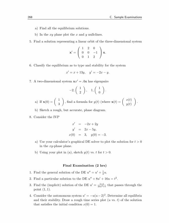
268 C. Sample Examinations

a) Find all the equilibrium solutions.

b) In the xy plane plot the x and y nullclines.

5. Find a solution representing a linear orbit of the three-dimensional system

x′ =

⎛⎝ 1 2 00 0 −10 1 2

⎞⎠x.

6. Classify the equilibrium as to type and stability for the system

x′ = x + 13y, y′ = −2x − y.

7. A two-dimensional system xx′ = Ax has eigenpairs

−2,

(12

), 1,

(10

).

a) If x(0) =(

13

), find a formula for y(t) (where x(t) =

(x(t)y(t)

).

b) Sketch a rough, but accurate, phase diagram.

8. Consider the IVP

x′ = −2x + 2y

y′ = 2x − 5y,

x(0) = 3, y(0) = −3.

a) Use your calculator’s graphical DE solver to plot the solution for t > 0in the xy-phase plane.

b) Using your plot in (a), sketch y(t) vs. t for t > 0.

Final Examination (2 hrs)

1. Find the general solution of the DE u′′ = u′ + 12u.

2. Find a particular solution to the DE u′′ + 8u′ + 16u = t2.

3. Find the (implicit) solution of the DE u′ = 1+t3tu2+t that passes through the

point (1, 1).

4. Consider the autonomous system u′ = −u(u−2)2. Determine all equilibriaand their stability. Draw a rough time series plot (u vs. t) of the solutionthat satisfies the initial condition x(0) = 1.


5. Consider the nonlinear system

x′ = 4x − 2x2 − xy, y′ = y − y2 − 2xy.

Find all the equilibrium points and determine the type and stability of theequilibrium point (2, 0).

6. An RC circuit has R = 1, C = 2. Initially the voltage drop across thecapacitor is 2 volts. For t > 0 the applied voltage (emf) in the circuit isb(t) volts. Write down an IVP for the voltage across the capacitor and finda formula for it.

7. Solve the IVPu′ + 3u = δ2(t) + h4(t), u(0) = 1.

8. Use eigenvalue methods to find the general solution of the linear system

x′ =(

2 0−1 2

)x.

9. In a recent TV episode of Miami: CSI, Horatio took the temperature of amurder victim at the crime scene at 3:20 A.M. and found that it was 85.7degrees F. At 3:50 A.M. the victim’s temperature dropped to 84.8 degrees.If the temperature during the night was 55 degrees, at what time was themurder committed? Note: Body temperature is 98.6 degrees; work in hours.

10. Consider the model u′ = λ2u − u3, where λ is a parameter. Draw thebifurcation diagram (equilibria solutions vs. the parameter) and determineanalytically the stability (stable or unstable) of the branch in the firstquadrant.

11. Consider the IVP u′′ =√

u + t, u(0) = 3, u′(0) = 1. Pick step size h = 0.1and use the modified Euler method to find an approximation to u(0.1).

12. A particle of mass m = 1 moves on the x-axis under the influence of apotential V (x) = x2(1 − x).

a) Write down Newton’s second law, which governs the motion of theparticle.

b) In the phase plane, find the equilibrium solutions. If one of the equi-libria is a center, find the type and stability of all the other equilibria.

c) Draw the phase diagram.

D. Solutions and Hints to Selected Exercises 271

DSolutions and Hints to Selected Exercises

CHAPTER 1

Section 1.1

2. Try a solution of the form u = atm and determine a and m.

4. Try a solution of the form u = at2 + bt + c.

6. u′ = u/3 + 2te3t.

8. (a) linear, nonautonomous; (b) nonlinear, nonautonomous; (c) nonlinear,autonomous; (d) linear autonomous.

9. The derivative of√

u is 1/(2√

u), which is not continuous when u = 0.

12. The slope field is zero on u = 0 and u = 4.

13. The nullclines are the horizontal lines u = ±1. The slope field is −3 on thelines u = ±2.

15. The nullclines are u = 0 and u = 4√

t.

16. Hint: at a positive maximum u′′ < 0, and so u′′ − u < 0, a contradiction.

17. Show the derivative of the expression is zero. In the uu′ plane the curvesplot as a family of hyperbolas.

18. Use the quotient rule to show the time derivative of u1/u2 is zero.

272 D. Solutions and Hints to Selected Exercises

Section 1.2

1. u = 12 sin(t2) + C. And u(0) = C = 1.

2. u = 23 t3/2 + 2

√t + C is the general solution.

5. u(t) =∫ t

1 e−s√

sds.

6 . y = − 14e−4t + C.

8. ddt (erf(sin t)) = erf ′(sin t) cos t = 2√

πe− sin2 t cos t.

9. (a) If the equation is exact, then f = ht and g = hu. Then fu = htu =hut = gt. (b)(i) fu = 3u2 = gt, and so the equation is exact. Then ht = u3

implies h = tu3 + φ(u). Then hu = 3tu2 + φ′(u) = 3tu2. Hence, φ′(u) = 0,or φ(u) = C1. Therefore h = tu3 + C1 = C2, or tu3 = C.

11. Take the derivative and use the fundamental theorem of calculus to getu′ = −2e−t + tu, u(0) = 1.

Section 1.3.1

1. Use k = mg/L.

3. The equation is mv′ = −F , v(0) = V with solution v = −(F/m)t+V . Thenx =

∫vdt = −(F/2m)t2 + V t.

6. Mass times acceleration equals force, or ms′′ = −mg sin θ. But s = lθ, somlθ′′ = −mg sin θ.

7. (a) ω =√

g/l. (b) 2.2 sec.

8. The x and y positions of the cannonball are x = (v cos θ)t, y = − 12gt2 +

(v sin θ)t + H, where θ is the angle of elevation of the cannon.

Section 1.3.2

1. The equilibria are p = 0 (stable), p = a (unstable), p = K (stable).

2. Find the equilibria by setting − rK p2 + rp−h = 0 and use the quadratic for-

mula. We get a positive equilibrium only when r ≥ 4h/K. If r = 4h/K thesingle equilibrium is semi-stable, and if r > 4h/K the smaller equilibriumis unstable and the larger one is stable.

3. r has dimensions 1/time, and a has dimensions 1/population. The maxi-mum growth rate occurs at p = 1/a. There is no simple formula for theantiderivative

∫eap

p dp.

4. Maximum length is a/b.


6. (a) 2√

u = t+C; (b) u = ln√

2t + C; (c) u = tan(t+C); (d) u = Ce3t +a/3;(e) 4 lnu + 0.5u2 = t + C; (f)

√π

2 erf(u2) = t + C.

9. The amount of carbon-14 is u = u0e−kt; 13, 301 years.

10. 35,595.6 years.

11. N ′ = bFT N(1 − cN/FT ) (a logistics type equation with carrying capacityFT /c).

12. R = k is asymptotically stable. The solution is R(t) = k exp(Ce−at).

13. p = m is unstable. If p(0) < m then population becomes extinct, and ifp(0) > m then it blows up.

14. I ′ = aI(N − I), which is logistics type. The asymptotically stable equilib-rium is I = N .

Section 1.3.3

1. p′ = 0.2p(1 − p/40) − 1.5 with equilibria p = 10 (unstable) and p = 30(stable). If p(0) ≤ 10 then the population becomes extinct.The populationwill likely approach the stable equilibrium p = 30.

2. (a) u = 0 (unstable), u = 3 (stable). (c) u = 2 (stable), u = 4 (unstable).

3. (a) Equilibria are u = 0 and u = h. We have fu(u) = h − 2u, and sofu(0) = h and fu(h) = −h. If h > 0 then u = 0 is unstable and u = h isstable; if h < 0 then u = 0 is stable and u = h is unstable. If h = 0 thereis no information from the derivative condition. A graph shows u = 0 issemi-stable.

7. Hint: Plot h vs. u instead of u vs. h.

Section 1.3.4

1. h = ln√

11/4. The solid will be 2◦ at time 2 ln(1/11)/ ln(4/11).

2. About 1.5 hours.

5. k is 1/time, q is degrees/time, and θ, Te, T0 are in degrees. The dimensionlessequation is dψ

dτ = −(ψ − 1) + ae−b/ψ, with b = θ/Te and a = q/kTe.

Section 1.3.5

1. C(t) = (C0 − Cin)e−qt/V + Cin.

2. The equation is 100C ′ = (0.0002)(0.5) − 0.5C.

5. The equilibrium C∗ = (−q +√

q2 + 4kqV Cin)/2kV is stable.


7. C ′ = −kV C gives C = C0e−kV t. The residence time is T = − ln(0.1)/kV.

8. C ′ = − aCb+C + R has a stable equilibrium C∗ = Rb/(a − R), where a > R.

The concentration approaches C∗.

9. a′ = −ka(a − a0 + b0); a → a0 − b0.

10. (b) Set the equations equal to zero and solve for S and P . (c) With valuesfrom part (b), maximize aV Pe.

Section 1.3.6

1. q(t) = 6 − e−2t, I(t) = 2e−2t.

3. The initial condition is I ′(0) = (−RI(0) + E(0))/L. The DE is LI ′′ + RI ′ +(1/C)I = E′(t).

5. Substitute q = A cos ωt into Lq′′ + (1/C)q = 0 to get ω = 1/√

LC, A

arbitrary.

6. I ′′ + 12 (I2 − 1)I ′ + I = 0.

7. LCV ′′c + RCV ′

c + Vc = E(t).

CHAPTER 2

Section 2.1

1. (c) u = tan(12 t2 + t + C). (d) ln(1 + u2) = −2t + C.

2. u = ln( t3

3 + 2); interval of existence is (−61/3,∞).

4. The interval of existence is (−√5/3,

√5/3).

6. The general solution is (u−1)1/3 = t2 +C. If u = 1 for all t, then t2 +C = 0for all t, which is impossible.

8. Integrate both sides of the equation with respect to t. For example,∫

(u′1/u1)dt =

lnu1 + C.

9. y′ = F (y)−yt . Using y = u/t the given DE can be converted to y′ = 4−y2

ty ,

which is separable.

10. u(t) = −e−3t + Ce−2t.

11. u(r) = −p4r2 + a ln r + b.

12. u(t) = u0 exp(−at2

2 ). The maximum rate of conversion occurs at time t =1/

√a.


13. The IVP is v′ = −32 − v2/800, v(0) = 160.

14. The governing equation is u′ = −k/u, with solution u(x) =√

C − 2kt.

16. u(t) = u0 exp(∫ t

ap(s)ds).

17. m is 1/time, b is 1/grasshoppers, and a is 1/(time · spiders). The dimen-sionless equation is dh

dτ = −h − λh1+h . The population h approaches zero as

t → ∞. Separate variables.

18. (a) 1 − e−mt; e−ma − e−mb. (b) S(t) = exp(∫ t

0 m(s)ds).

Section 2.2

1. u(t) = 13 t2 + C

t .

2. u(t) = Ce−t + 12et.

4. q(t) = 10te−5t. The maximum occurs at t = 1/5.

5. The equation becomes y′ + y = 3t, which is linear.

6. The equation for y is y′ = 1 + y2. Then y = tan(t + C), u = tan(t + C) − t.

7. u(t) = et2(C +√

π2 erf(t)).

8. u(t) = (u0 + q/p)ept − q/p.

11. (b) Let y = u−1. Then y′ = −y − e−t and y = Ce−t − 12et. Then u =

(Ce−t − 12et)−1. (c) y′ = −3y/t + 3/t; y = 1 + C/t3; u = y1/3.

12. The vat empties at time t = 60. The governing equation is (60 − t)u′ =2 − 3u.

14. S∗ = raM/(aM + rA).

15. x′ = kx(N − x), which is similar to the logistics equation.

16. The IVP is T ′ = −3(T − 9 − 10 cos(2πt)), T (0) = 12.

18. P ′ = N −P. The stable equilibrium is P = N , so everyone hears the rumor.

19. mv′ = mg − 2t+1v, v(0) = 0.

20. (a) S∗ = IP/(I + E). (b) The equation is linear: S′ = − 1P (I + E)S + I.

The general solution is S(t) = S∗ + Ce− tP (I+E).(c) Use the formula for S∗

for each island and compare.

21 . Ex.2: u′ + u = et has integrating factor et. Multiply by the factor to get(uet)′ = e2t; integrate to get uet = 1

2e2t + C.


Section 2.3

1. The Picard iteration scheme is un+1(t) =∫ t

0 (1 + un(s)2)ds, u0(t) = 0. Itconverges to tan t = t + 1

3 t3 + 215 t5 + · · · .

2. The Picard iteration scheme is un+1(t) = 1+∫ t

0 (s−un(s))ds, u0(t) = 1. Weget u1(t) = 1 − t + t2/2 + · · · , etc.

Section 2.4

2. u(t) = esin t.

4. The exact solution is un = u0(1−hr)n. If h > 1/r then the solution oscillatesabout zero, but the solution to the DE is positive and approaches zero. Sowe require h < 1/h.

7. u = e−t. Roundoff error causes the exponentially growing term Ce5t in thegeneral solution to become significant.

CHAPTER 3

Section 3.1

1. V (x) = x2/2 − x4/4.

2. mx′′x = F (x)x′. But ddtV (x) = dV

dx x′ = −F (x)x′ and mx′′x′ = m ddt (x

′)2 =2mx′x′′. Hence 1

2m ddt (x

′)2 = − ddtV (x). Integrating both sides gives 1

2m(x′)2 =V (x) + C, which is the conservation of energy law.

5. (a) Make the substitution v = x′. The solution is x(t) = a/t + b. (b) Makethe substitution v = x′. The solution is

∫dx

a+0.5xx = t + b.

Section 3.2

1. (a) u = e2t(a + bt). (d) u(t) = a cos 3t + b sin 3t. (e) u(t) = a + be2t. (f)u(t) = a cosh(

√12t) + b sinh(

√12t).

4. The solution is periodic if a = 0 and b > 0; the solution is a decayingoscillation if a < 0 and a2 < b; the solution decays without oscillation ifa < 0 and a2 ≥ b.

5. L = 14 (critically damped), L < 1

4 (over damped), L > 14 , (under damped).

6. Critically damped when 9a2 = 4b, which plots as a parabola in ab parameterspace.

7. u′′ + 2u′ − 24u = 0.


8. u′′ + 6u′ + 9u = 0.

9. u′′ + 16u = 0.

10. A = 2, B = 0.

12. I(t) =√

10 sin(t/√

10).

Section 3.3.1

1. (a) up = at3 + bt2 + ct + d. (b) up = a. (d) up = a sin 7t + b cos 7t. (f)up = (a + bt)e−t sin πt + (c + dt)e−t cos πt.

2. (c) up = t2 − 2t + 2. (e) up = 92e−t.

4. The general solution is u(t) = c1 + c2e2t − 2t.

5. Write sin2 t = 12 (1 − cos 2t) and then take up = a + b cos 2t + c sin 2t.

7. u(t) = a cos 50t + b sin 50t + 0.02.

8. The circuit equation is 2q′′ + 16q′ + 50q = 110.

Section 3.3.2

2. u(t) = c1 cos 4t + c2 sin 4t + 132 cos 4t + 1

8 t sin 4t.

3. L = 1/Cβ2.

Section 3.4

1. (b) u(t) = 2 ln t.

2. β = 1.

7. u(t) = tan(t + π/4).

9. The other solution is teat.

11. 1√tsin t.

14. Take the derivative of the Wronskian expression W = u1u′2 −u′

1u2 and usethe fact that u1 and u2 are solutions to the differential equation to showW ′ = −p(t)W. Solving gives W (t) = W (0) exp(− ∫

p(t)dt), which is alwaysof one sign.

16. The given Riccati equation can be transformed into the Cauchy–Eulerequation u′ − 3

t u′ = 0.

17. (b) up = − cos t ln((1 + sin t)/ cos t). (c) Express the particular solution interms of integrals. (e) up = t3/3.

18. (a) tp(t) = t · t−1 = 1, and t2q(t) = t2(1 − k2

t2 ) = t2 − k2, which are bothpower series about t = 0.


Section 3.5

2. u(x) = − 16x3 + 1

240x4 + 1003 x. The rate that heat leaves the right end is

−Ku′(20) per unit area.

4. There are no nontrivial solutions when λ ≤ 0. There are nontrivial solutionsun(x) = sinnπx when λn = n2π2, n = 1, 2, 3, ....

5. u(x) = 2π√

x.

6. Integrate the steady-state heat equation from 0 to L and use the fundamentaltheorem of calculus. This expression states: the rate that heat flows in atx = 0 minus the rate it flows out at x = L equals the net rate that heat isgenerated in the bar.

7 . When ωL is not an integer multiple of π.

8. λ = −1 − n2π2, n = 1, 2, . . ..

10. Hint: this is a Cauchy–Euler equation. Consider three cases where the val-ues of λ give characteristic roots that are real and unequal, real and equal,and complex.

Section 3.6

1. (a) u(t) = c1+c2 cos t+c3 sin t. (b) u(t) = c1+et/2(c2 cos√

32 t+c3 sin

√3

2 t)+c4e

−t + t. (c) u(t) = c1 + c2t + c3 cos t + c4 sin t.

5. u(t) = e3t(c1 cos t + c2 sin t) + te3t(c3 cos t + c4 sin t).

Section 3.7

1. (b) u(t) = CeRt. (c) u(t) = Ce− sin t − 1. (e) u(t) =√

t(c1 cos(√

72 ln t) +

c2 sin(√

72 ln t)). (g) u(t) = −4t2 + 6t + C. (i) A Bernoulli equation. (k)

x(t) = ± ∫dt√

A−2t+ B. (l) Bernoulli equation. (m) ± ∫ u

0dw√

A−2w= t + B.

(n) Homogeneous equation. (p) Exact equation.

2. u(t) = (12 − sin t)−1, −7π/6 < t < π/6.

5. If a ≤ 0 then u = a is the only equilibrium (unstable). If 0 < a < 1 thenthere are three equilibria: u = ±√

a (unstable), and u = a (stable). Ifa = 1 then u = 1 is unstable. If a > 1 then u =

√a (stable), u = a, −√

a

(unstable).

6. r(t) = −kt + r0.

7. p = 0 (unstable); p = K (stable).

11. u(t) = exp(t2 + C/t2).


12. u(t) = t − 3t ln t + 2t2.

CHAPTER 4

Section 4.1

1. U(s) = 1s (e−s − e−2s).

2. Integrate by parts twice.

3. L[sin t] = 11+s2 ; L[sin(t − π/2)] = − s

1+s2 ; L[hπ/2(t) sin(t − π/2)] =s

1+s2 e−πs/2.

4. 2!(s+3)3 .

5. Use sinh kt = 12 (ekt − e−kt).

7. 1s+1e−2(s+1).

9. et2 is not of exponential order; the improper integral∫ ∞0

1t e

−stdt does notexist at t = 0. Neither transform exists.

11. 1s

11+e−s .

12. Hint: Use the definition of the Laplace transform and integrate by partsusing e−st = − 1

sddt (e

−st).

13. Hint: ddsU(s) =

∫ ∞0 u(t) d

dse−stdt.

14. ln(√

(s + 1)/(s − 1)), s > 1.

15. Integrate by parts.

17. (a) Integrate by parts. Change variables in the integral to write Γ ( 12 ) =

2∫ ∞0 e−r2

dr.

Section 4.2

2. (c) 13 t3e5t. (d) 7h4(t).

3. (c) u(t) = 35e3t + 7

5e−2t. (d) u(t) = et sin t. (f) u(t) = 1. (i) 32 cosh(

√2t) − 1

2 .

4. Solve for the transforms X = X(s), Y = Y (s) in sX = X − 2Y − 1s2 ,

sY = 3X + Y , and then invert.

5. dn

dsn U(s) =∫ ∞0 u(t) dn

dsn e−stdt.

Section 4.3

1. 12 t sin t.


2. 112 t4.

3. u(t) = u(0)eat +∫ t

0 ea(t−s)q(s)ds.

5. u(t) = 1ω

∫ t

0 sinh(t − s)f(s)ds.

7. u(t) =∫ t

3 f(t − s)ds.

8. u(t) =∫ t

0 (et−s − 1)f(s)ds.

9. U(s) = F (s)1−K(s) .

10. (a) u(t) = sin(t); (b) u(t) = 0.

11. The integral is a convolution.

Section 4.4

1. 2s (e−3s − e−4s).

2. e−3s( 2s3 + 6

s2 + 9s ).

3. 16 t3e2t.

4. Note f(t) = 3 − h2(t) + 4hπ(t) − 6h7(t).

5. t − h4(t)(t − 4).

7. u(t) = et on [0, 1]; u(t) = e−2e et + 2 on t > 1.

8. Solve q′′ + q = t + (9 − t)h9(t).

10. u(t) = 1, 0 ≤ t ≤ 1; u(t) = − cos πt, t > 1.

13. 2 − ∑∞n=1(1)nhn(t).

Section 4.5

1. 1/e2.

3. u(t) = sinh(t − 5)h5(t).

4. u(t) = sin(t − 2)h2(t).

5. u(t) = h2(t) + δ3(t).

6. u(t) = 12 cos[2(t − 2)]h2(t) − cos[2(t − 5)]h5(t).

7. v(t) =∑∞

n=0 sin(t − nπ)hnπ(t).


CHAPTER 5

Section 5.1

1. The orbit is an ellipse (taken counterclockwise).

2. The tangent vector is x′(t) = (2,−3)Tet and it points in the direction(2,−3)T.

3. x(t) = 8+2e−5t, y(t) = 8− 8e−5t. Over a long time the solution approachesthe point (equilibrium) (8, 8).

4. Multiply the first equation by 1/W , the second by 1/V, and then add to getx′/W + y′/V = 0, or x/W + y/V = C. Use y = V (C − x/W ) to eliminatey from the first equation to get a single equation in the variable x, namely,x′ = −q(1/V +1/W )x+ qC. The constant C is determined from the initialcondition.

6. Solve the equation x′′ + 12x′ + 2x = 0 to get a decaying oscillation x = x(t).

In the phase plane the solution is a clockwise spiral entering the origin.

7. The system is q′ = I, I ′ = −4q. We have q(t) = 8 cos 2t and I(t) =−16 sin 2t. Both q and I are periodic functions of t with period π, andin the phase plane q2/64 + I2/256 = 1, which is an ellipse. It is traversedclockwise.

Section 5.2

1. det(A − λI) = λ2 − 5λ − 2.

2. x = 3/2, y = 1/6.

4. det(A − λI) = λ2 − 5λ − 2 = 0, so λ = 52 ± 1

2

√33.

5. det A = 0 so A−1 does not exist.

6. If m = −5/3 then there are infinitely many solutions, and if m �= −5/3, nosolution exists.

7. m = 1 makes the determinant zero.

8. Use expansion by minors.

10. det(A) = −2, so A is invertible and nonsingular.

11. x = a(2, 1, 2)T, where a is any real number.

12. Set c1(2,−3)T+c2(−4, 8)T = (0, 0)T to get 2c1−4c2 = 0 and −3c1+8c2 = 0.This gives c1 = c2 = 0.


13. Pick t = 0 and t = π.

14. Set a linear combination of the vectors equation to the zero vector and findcoefficients c1, c2, c3.

16. r1(t) plots as an ellipse; r2(t) plots as the straight line y = 3x. r2(t) plotsas a curve approaching the origin along the direction (1, 1)T. Choose t = 0to get c1 = c3 = 0, and then choose t = 1 to get c2 = 0.

Section 5.3

1. For A the eigenpairs are 3, (1, 1)T and 1, (2, 1)T. For B the eigenpairs are0, (3,−2)T and −8, (1, 2)T. For C the eigenpairs are ±2i, (4, 1 ∓ i)T.

2. x = c1(1, 5)Te2t + c2(2,−4)Te−3t. The origin has saddle point structure.

3. The origin is a stable node.

4. (a) x = c1(−1, 1)T e−t + c2(2, 3)T e4t (saddle), (c) x = c1(−2, 3)T e−t +c2(1, 2)T e6t (saddle), (d) x = c1(3.1)T e−4t + c2(−1, 2)T e−11t (stable node),(f) x(t) = c1e

t(cos 2t − sin 2t) + c2et(cos 2t + sin 2t), y(t) = 2c1e

t cos 2t +2c2e

t sin 2t (unstable spiral), (h) x(t) = 3c1 cos 3t + 3c2 sin 3t, y(t) =−c1 sin 3t + c2 cos 3t (center).

6. (a) Equilibria consist of the entire line x − 2y = 0. (b) The eigenvalues are0 and 5; there is a linear orbit associated with 5, but not 0.

7. The eigenvalues are λ = 2 ± √a + 1; a = −1 (unstable node), a < −1

(unstable spiral), a > −1 (saddle).

9. The eigenvalues are never purely imaginary, so cycles are impossible.

11. There are many matrices. The simplest is a diagonal matrix with −2 and−3 on the diagonal.

13. The system is v′ = w, w′ = −(1/LC)v − (R/L)w. The eigenvalues areλ = −R/2L ± √

R2/4L2 − 1/LC. The eigenvalues are complex whenR2/4L < 1/C, giving a stable spiral in the phase plane, representing de-caying oscillations in the system.

14. The eigenvalues are −γ ± i. When γ = 0 we get a cycle; when γ > 0 we geta stable spiral; when γ < 0 we get an unstable spiral.

Section 5.4

2. The equations are V1x′ = (q + r)c − qx − rx, V2y

′ = qx − qy. The steady-state is x = y = c. When freshwater enters the system, V1x

′ = −qx − rx,

V2y′ = qx − qy. The eigenvalues are both negative (−q and −q − r), and

therefore the solution decays to zero. The origin is a stable node.


5. A fundamental matrix is

Φ(t) =(

2e−4t −e−11t

3e−4t 2e−11t

).

The particular solution is xp = −( 942 , 1

21 )Te−t.

6. det A = r2r3 > 0 and tr(A) = r1−r2−r3 < 0. So the origin is asymptoticallystable and both x and y approach zero. The eigenvalues are λ = 1

2 (tr(A)±12

√tr(A)2 − 4 detA.

7. In the equations in Problem 6, add D to the right side of the first (x′) equa-tion. Over a long time the system will approach the equilibrium solution:xe = D/(r1 + r2 + r1r3/r2), ye = (r1/r2)xe.

Section 5.5

1. The eigenpairs of A are 2, (1, 0, 0)T; 6, (6, 8, 0)T; −1, (1,−1, 7/2)T. Theeigenpairs of C are 2, (1, 0, 1)T; 0, (−1, 0, 1)T; 1, (1, 1, 0)T.

2(a). x = c1

⎛⎝ 11−2

⎞⎠ e−2t + c2

⎛⎝ 3−32

⎞⎠ e4t + c3

⎛⎝ −110

⎞⎠ e2t.

2(b). x = c1

⎛⎝ 212

⎞⎠+c2

⎛⎝ cos 0.2t

sin 0.2t

− cos 0.2t − sin 0.2t

⎞⎠+c3

⎛⎝ − sin 0.2t

cos 0.2t

− cos 0.2t + sin 0.2t

⎞⎠ .

2(d). x = c1

⎛⎝ 101

⎞⎠ e2t + c2

⎛⎝ −101

⎞⎠ + c3

⎛⎝ 110

⎞⎠ et.

4. The eigenvalues are λ = 2, ρ ± 1.

CHAPTER 6

Section 6.1.1

1. y = Ce1/x, x(t) = (c1 − t)−1, y(t) = c2e−t.

2. y = 1x2+C . There are no equilibrium solutions. No solutions can touch the

x-axis.

3. Two equilibrium points: (√

4/5, 2√

4/5), (−√4/5,−2

√4/5). The vector

field is vertical on the circle of radius 2: x2 + y2 = 4. The vector fieldis horizontal on the straight line y = 2x.


4. (±1,−1). The vector field is vertical on the line y = −1 and horizontal onthe inverted parabola y = −x2.

5. (0, 0), (1, 1), and (4, 4).

6. (0, nπ), n = 0,±1,±2, ...

7. dV/dt = 2xx′ + 2yy′ = −2y4 < 0.

8. The equilibria are the entire line y = x; they are not isolated.

Section 6.1.2

1. There is no epidemic. The number of infectives decreases from its initialvalue.

2. I(t) increases to a maximum value, then S(t) decreases to the value S∗.

3. r = 1/3 and a = 0.00196. The average number of days to get the flu is about2.5 days.

4. r = 0.25 and a = 0.001, giving S∗ = 93. Also Imax = 77.

5. I ′ = aI(N − I) − rI. The equilibrium is I = aN − r.

8. x′ = rx − axy, y′ = −my + bxy − M.

9. The equilibria are (0, 0) and (m/b, k/a). The vector field shows that curvesveer away from the nonzero equilibrium, so the system could not coexistin that state.

10. S′ = −aSI − ν, aSI − rI.

11. S′ = −aSI + µ(N − S − I), I ′ = aSI − rI. The equilibria are (N, 0) andthe endemic state (r/a, I∗) where I∗ = µ(N − r/a)/(r + µ).

Section 6.2

4. Begin by writing the equation as u′ = v, v′ = −9u + 80 cos 5t.

6. The system is x′ = y, y′ = −x/2 + y/2 − y3/2.

7. The system is x′ = y, y′ = −2(x2 − 1)y − x.

8. S(0) = 465 with a = 0.001 and r = 0.2.

9. S′ = −aSI, I ′ = aSI − rI − qI.

Section 6.3

1. y = C(ex − 1).

2. y2 − x2 − 4x = C.


3. Equilibria are (0, 0) (a saddle structure) and (2, 4) (stable node) and null-clines: y = x2 and y = 2x.

4. a < 0 (no equilibria); a = 0 (origin is equilibrium); a > 0 (the equilibria are(−√

a/2, 0) and (√

a/2, 0), a stable node and a saddle).

6. (−1, 0) (stable spiral); (1, 0) (saddle).

8. (2, 4) (saddle); (0, 0) (stable node). The Jacobian matrix at the origin has azero eigenvalue.

10. tr(A) < 0, det A > 0. Thus the equilibrium is asymptotically stable.

11. See Exercise 7, Section 6.1.1.

12. The force is F = −1 + x2, and the system is x′ = y, y′ = −1 + x2.

The equilibrium (1, 0) is a saddle and (−1, 0) is a center. The latter isdetermined by noting that the orbits are 1

2y2 + x − 13x3 = E.

13. (a) dHdt = Hxx′ + Hyy′ = HxHy + Hy(−Hx) = 0. (c) The Jacobian matrix

at an equilibrium has zero trace. (e) H = 12y2 − x2

2 + x3

3 .

14. (0, 0) is a center.

15. (c) The eigenvalues of the Jacobian matrix are never complex.

16. (0, 0), (0, 12 ), and (K, 0) are always equilibria. If K ≥ 1 or K ≤ 1

2 then noother positive equilibria occur. If 1

2 < K ≤ 1 then there is an additionalpositive equilibrium.

17. a = 1/8 (one equilibrium); a > 1/8, (no equilibria); 0 < a < 1/8 (twoequilibria).

19. The characteristic equation is λ2 = f ′(x0). The equilibrium is a saddle iff ′(x0) > 0.

Section 6.4

2. There are no equilibrium, and therefore no cycles.

3. fx + gy > 0 for all x, y, and therefore there are no cycles (by Dulac’s crite-rion).

4. (1, 0) is always a saddle, and (0, 0) is unstable node if c > 2 and an unstablespiral if c < 2.

6. (0, 0) is a saddle, (±1, 0) are stable spirals.

7. The equilibria are H = 0, P = φ/a and H = εφc − a

b , P = cεb .


8. In polar coordinates, r′ = r(a−r2), θ′ = 1. For a ≤ 0 the origin is a stablespiral. For a > 0 the origin is an unstable spiral with the appearance of alimit cycle at r =

√a.

9. The characteristic equation is λ2 + kλ + V ′′(x0) = 0 and has roots λ =12 (−k ± √

k2 − 4V ′′(x0)). These roots are never purely imaginary unlessk = 0.

10. Use Dulac’s criterion.

11. Equilibria at (0, 0), (1, 1, ), and (4, 4).

Index

advertising model, 67AIDS, 60Airy’s equation, 105Allee effect, 37Allee, W. C., 37allometric growth, 59amplitude, 90analytic solution, 9antiderivative, 14approximate solution, 9asymptotic stability, 32asymptotic stability, global, 34asymptotic stability, local, 34attractor, 31, 32, 195augmented array, 173autonomous, 4autonomous equation, 11, 28, 31autonomous equations, 128

basin of attraction, 251batch reactor, 50beats, 105Bernoulli equation, 68, 128Bessel’s equation, 117bifurcation, 42, 241bifurcation diagram, 42bifurcation parameter, 42biogeography, 70boundary condition, 119boundary condition, flux, 120boundary condition, insulated, 120boundary value problem, 119budworm outbreaks, 38

carbon dating, 40Cauchy, A., 108Cauchy–Euler equation, 106, 128center, 190change of variables method, 46characteristic equation, 89, 106, 125, 186characteristic root, 89chemostat, 48compartmental model, 163competition model, 223complementary solution, 62conservation of energy, 25, 85, 212conservative force, 85constant of integration, 14constitutive relation, 24continuously stirred tank reactor, 48convolution, 146cooperative model, 223critically damped, 91

damped spring-mass equation, 25, 91delta function, 153determinant, 168difference quotient, 19differential equation, 2digestion model, 51dimensionless model, 34dimensions, 20direction field, 10Duffing equation, 232Dulac’s criterion, 246dynamical equation, 21

288 Index

eigenfunction, 121eigenpair, 185eigenvalue, 185eigenvalue problem, 185eigenvalues of an operator, 121eigenvector, 185eigenvector, generalized, 192electrical circuit, 51electromotive force (emf), 51epidemic model, 223equation of motion, 21equilibrium solution, 22, 30, 31, 180,

194, 211erf, 16error function, 16error, in a numerical algorithm, 78error, local, 79Euler method, 74, 230Euler’s formula, 90Euler, L., 74, 108exact equation, 18exponential order, 137extinction–explosion model, 40

finite difference method, 74fixed point iteration, 71Fourier’s law, 119Frobenius method, 111fundamental matrix, 198Fundamental Theorem of Calculus, 13

gamma function, 140general solution, 5Gompertz model, 40gradient system, 244Green’s theorem, 247growth rate, 28growth rate, per capita, 29growth–decay model, 36

Hamiltonian system, 244harvesting, 41heat conduction equation, 119heat loss coefficient, 45Heaviside function, 135Hermite’s equation, 115higher-order equations, 124Holling functional response, 222Holling, C., 221homogeneous, 61homogeneous differential equation, 59,

128Hooke’s law, 24hyperbolic functions, 94

implicit numerical method, 77impulse, 152independent solutions, 88initial condition, 6initial value problem, 6, 88, 160, 210integral equation, 19integrating factor, 70interval of existence, 7, 8isolated equilibrium, 32, 180, 194, 211

Jacobian matrix, 236Jung, C., 20

Kirchhoff’s law, 51

Laplace transform, 134Laplace transform, inverse, 137Laplace transforms, Table of, 157limit cycle, 239linear equation, 4linear independence of vectors, 175linearization, 235logistics model, 29Lotka, A., 220Lotka–Volterra equations, 217

MacArthur–Wilson model, 70Malthus model, 28Malthus, T., 28mathematical model, 19matrix, 165matrix inverse, 168matrix minor, 169mechanical-electrical analogy, 87Michaelis–Menten kinetics, 50modified Euler method, 78, 231Monod equation, 50multiplicity, 125

natural frequency, 90Newton’s law of cooling, 45Newton’s second law, 21, 84Newton, I., xiv, 21node, asymptotically stable, 188, 195node, degenerate, 192node, star-like, 192node, unstable, 188nonautonomous, 4nonhomogeneous, 62nonhomogeneous equations, 95nonlinear equation, 4nonsingular matrix, 168normal form, 4nullcline, 12, 194, 218numerical solution, 9

Index 289

Ohm’s law, 52one-parameter family, 5orbit, 85, 160, 179, 210orbit, linear, 182, 185order, 3order of a numerical method, 75over-damped, 91

parameter, 3partial fraction expansion, 142particular solution, 5pendulum equation, 26perturbation, 32phase, 90phase diagram, 86, 161, 211phase line, 30, 33phase plane, 85, 160, 179Picard iteration, 71Picard, E., 71piecewise continuous, 137Poincare, H., 249Poincare–Bendixson Theorem, 249potential energy, 85, 212power series solutions, 109predator–prey model, 217predictor–corrector method, 78pure time equation, 13, 127

qualitative method, 9

RC circuit, 53RCL circuit, 52RCL circuit equation, 53reduction of order, 112refuge model, 227regular singular point, 111repeller, 31, 32, 195resonance, 102resonance, pure, 104Riccati equation, 116Ricker population law, 38Rosenzweig–MacArthur model, 223row reduction, 172Runge–Kutta method, 78, 231

saddle point, 183, 189, 195semi-stable, 34separation of variables, 36, 55, 127separatrix, 183, 237singular matrix, 168

sink, 195SIR model, 223SIS model, 227slope field, 10solution, 4solution, explicit, 56solution, general, 88, 124solution, implicit, 56solution, numerical, 75solution, singular, 59source, 195spiral, asymptotically stable, 190, 195spiral, unstable, 190, 195spring constant, 24spring-mass equation, 24stability analysis, local, 235, 241stability, global, 215stability, local, 215stable, asymptotically, 215stable, neutrally, 195, 215steady-state response, 66, 100steady-state solution, 22stepsize, 74, 230stiffness, spring, 24structural instability, 81survivorship function, 61

technology transfer, 69thermal conductivity, 119time domain, 134time scale, 34time series, 1, 179trace, 186transform domain, 134transient response, 66, 100tumor growth model, 40

under-damped, 91undetermined coefficients, 96, 129units, 20unstable, 32, 215

van der Pol equation, 232variation of constants, 62variation of parameters, 114, 129, 199vector field, 161Verhulst, P., 29Volterra, V., 220

Wronskian, 114

References - link.springer.com3A978-0-387-29930-3%2F1… · R. V. Churchill, 1972. Operational...

Documents

Transcript of References - link.springer.com3A978-0-387-29930-3%2F1… · R. V. Churchill, 1972. Operational...