Reexamination of Real Business Cycles in A SmallOpen Economy�

Jang-Ting GuoUniversity of California, Riversidey

Zuzana Jankoz

University of Calgary

January 29, 2008

Abstract

Standard dynamic small open economy models have predicted a counterfactual perfectlypositive correlation between output and hours worked over the business cycle. In addi-tion, this class of models exhibits a weak internal propagation mechanism. To addressthese anomalies, this paper incorporates intertemporally non-separable labor supply andvariable capital utilization into the canonical Mendoza model with adjustment costs of netinvestment. Our analysis shows that a dynamic, technology-shock driven small open econ-omy model with internal habit formation in labor hours and endogenous capital utilizationis able to account for the main real business cycle regularities of Canada after 1981.

Keywords: Real Business Cycles, Small Open Economy, Capital Utilization, Habit Forma-tion.

JEL Classi�cation: E32, F41.

�We thank Hung-Ju Chen, Dean Corbae, Yu-Ning Hwang, Hashmat Khan, Francisco Gonzalez, Sharon Har-rison, Enrique Mendoza, Eric Leeper, Marc-André Letendre, Stephanie Schmitt-Grohé, Richard Suen, MartinUribe and seminar participants at University of Calgary, the 2007 Annual Meetings of the Canadian EconomicsAssociation, the 2007 North American Summer Meeting of the Econometric Society, and the 2007 Far EasternMeeting of the Econometric Society for helpful discussions and comments. Of course, all remaining errors areour own.

yCorresponding Author. Department of Economics, 4128 Sproul Hall, University of California, Riverside,CA, 92521, USA, Phone: (951) 827-1588, Fax: (951) 827-5685, E-mail: guojt@ucr.edu.

zDepartment of Economics, University of Calgary, 2500 University Drive, N.W., Calgary, Alberta, CanadaT2N 1N4, Phone: (403) 220-6101, Fax: (403) 282-5262, E-mail: zjanko@ucalgary.ca.

1 Introduction

Since the in�uential work of Mendoza (1991), it is now well known that dynamic stochastic

general equilibrium models, speci�cally the real-business-cycle approach, can successfully ex-

plain some important stylized facts of a small open economy with incomplete asset markets in

which domestic households only have access to a one-period risk free foreign bond. In partic-

ular, Mendoza�s model correctly predicts that the correlation between savings and investment

rates is positive, and that the balance of trade moves countercyclically with output over the

business cycle. As pointed out by Correia, Neves and Rebelo (1995), the ability of this class

of models to mimic key international indicators of a small open economy depends crucially on

adopting the period utility function postulated by Greenwood, Hercowitz and Hu¤man (GHH,

1988) whereby there is no income e¤ect associated with the household�s labor supply decision.

As a result, the elasticity of intertemporal substitution in hours worked (or leisure) is zero.

On the other hand, studies in this line of research have produced a set of clearly identi�ed

anomalies. One of the most robust puzzles, caused by the GHH preferences combined with a

Cobb-Douglas production technology, is the perfectly positive correlation between detrended

GDP and labor hours. Motivated by this counterfactual inconsistency, Schmitt-Grohé and

Uribe�s (2003, section 8:1) sensitivity analysis shows that a dynamic small open economy

model which allows for a wealth e¤ect in labor supply does not perform as well as that under

the GHH utility formulation, e.g., the model-generated time series of consumption is too

smooth compared to the observed variability, and the trade balance becomes procyclical.

Moreover, this type of small open real business cycle models, similar to the correspond-

ing closed-economy version, exhibits a weak internal propagation mechanism. Using the

productivity-disturbance process that Letendre (2004) estimates from Canadian quarterly

data since 1981, we �nd that in Mendoza�s model with capital adjustment costs, output is

less volatile than that observed in the actual economy; moreover, the coe¢ cients of serial

correlation in GDP, investment and work e¤ort are all statistically lower than their empirical

counterparts.1 In addition, this benchmark speci�cation exaggerates the negative correlations

between GDP and the ratios of trade balance and current account to output.

To address the above-mentioned anomalies, this paper incorporates intertemporally non-

1By contrast, this anomaly does not arise in Mendoza (1991) and Schmitt-Grohé and Uribe (2003) becausethey calibrate the persistence parameter for the technology shock and the standard deviation of its innovationsso that the resulting arti�cial time series of output displays the same volatility and �rst-order serial correlationas those in the Canadian annual data, 1946� 1985.

1

separable labor supply (or leisure) and variable capital utilization into Mendoza�s one-sector,

dynamic small open economy model with adjustment costs of net investment. Furthermore, in

order to highlight the cyclical e¤ects of these two additional features, productivity disturbances

are postulated to be the only driving process for generating macroeconomic �uctuations. Most

studies in the existing literature employ the GHH preferences that are separable over time,

which in turn contributes to the perfectly positive correlation between output and employ-

ment. To overcome this counterfactual result, as in Kydland and Prescott (1982) and Lettau

and Uhlig (2000) for closed-economy real business cycle models, we consider a time nonsepa-

rable utility function that exhibits non-zero elasticities of substitution in hours worked across

di¤erent periods. In addition, based on the empirical �ndings of Hotz, Kydland and Sedlacek

(1988), Eichenbaum, Hansen and Singleton (1988) and Wen (1998), the formulation with ei-

ther intertemporal substitutability (i.e. the fatigue e¤ects) or complementarity (i.e. internal

habit formation) of work e¤ort is examined in our analyses.2

We also follow Letendre (2004) and strengthen the model�s endogenous propagation mech-

anism by allowing for variable capital utilization. Speci�cally, a more intensive utilization of

capital is assumed to accelerate its rate of depreciation. In a symmetric equilibrium, the social

technology displays a larger elasticity of output with respect to both the technology shock

and labor inputs than those in the original Mendoza economy. As a result, varying capital

utilization ampli�es the business-cycle e¤ects of productivity disturbances since it provides an

additional margin to change output. It follows that as in closed-economy real business cycle

models (see Burnside, Eichenbaum and Rebelo, 1993; Burnside and Eichenbaum, 1996, among

others), smoother technology shocks are needed to match the observed volatility of GDP.

We obtain simulated second moments and impulse response functions from six versions

of our model economy, and then compare them with the H-P �ltered, post-1981 Canadian

quarterly data documented by Letendre (2004). The �rst three models exhibit time-invariant

capital utilization and depreciation rates. As discussed earlier, our benchmark speci�cation

(Model 1) corresponds to Mendoza�s one-sector, dynamic small open economy model subject

to the productivity-disturbance process estimated by Letendre (2004). When the household�s

current and previous choices of hours worked are included in its period utility function either

as substitutes (Model 1a) or complements (Model 1b), we show that both models perform

2Letendre (2004) incorporates internal habit formation in consumption into the Mendoza economy withcapital adjustment costs. In this case, the perfectly positive correlation between output and hours workedremains unchanged.

2

no worse than the baseline con�guration at matching the contemporaneous correlations with

GDP; whereas the model�s predictions of the serial correlations in key macroeconomic ag-

gregates are signi�cantly improved because of the presence of labor persistence. Moreover,

allowing for intertemporal substitution raises the elasticity of labor supply with respect to

changes in its marginal productivity, which in turn leads to more variable hours worked and

GDP compared to those in Model 1. However, output volatility in this case remains lower

than what the Canadian economy displays. By contrast, intertemporal complementarity of

labor hours dampens the cyclical e¤ects of technology shocks, thus work e¤ort and output

become less variable in comparison with the benchmark Model 1.

With a time nonseparable preference formulation, the household�s period-t labor supply de-

cision takes into account its expected in�uence on future utilities, hence GDP and hours worked

are no longer perfectly correlated. Compared to Model 1, intertemporal substitutability gen-

erates higher initial increases of labor hours and output in response to a positive transient

technology shock, and then they display similar oscillatory dynamics before falling back grad-

ually to the steady state. As a result, the correlation between output and employment remains

statistically too high (0:99) vis-á-vis the Canadian data (0:91). On the contrary, intertemporal

complementarity leads to weaker initial responses of hours worked and output than those in

Model 1. The associated sluggish movement in the household�s labor supply decision makes

GDP and work e¤ort continue to rise after the impact period in spite of a decreasing marginal

productivity of labor, thereby generating hump-shaped impulse response functions. Moreover,

the subsequent adjustment paths of hours worked and output are not closely synchronized in

that labor now becomes a lagging variable of the business cycle. This will result in a lower

correlation coe¢ cient between GDP and employment (0:92) that is remarkably close to the

Canadian economy.

The remaining three models exhibit time-varying capital utilization and depreciation rates,

and they are driven by a smoother technology-shock process that Letendre (2004) also esti-

mates from the post-1981 Canadian quarterly data. It turns out that even with a 13:36%

reduction in the standard deviation of the driving productivity innovations, all variables in

these speci�cations display substantially higher volatilities than their �xed-utilization coun-

terparts. Moreover, since the persistence parameter of productivity disturbances remains

virtually unchanged, incorporating variable capital utilization does not signi�cantly in�uence

the model�s predictions of autocorrelations, contemporaneous correlations with output and

3

the savings-investment comovement.

As in the benchmark Model 1, the no-labor-persistence Models 2 continues to show a

counterfactual perfectly positive correlation between output and employment, and statistically

lower serial correlations in GDP and hours worked than those observed in the data. On the

other hand, Model 2a (with intertemporal substitutability) �overshoots� the volatilities of

output, consumption and investment, and underpredicts the autocorrelations in GDP and

labor hours. By contrast, the formulation with intertemporal complementarity (Model 2b)

produces a statistically close match with the observed variabilities of output, consumption,

investment and the trade-balance-to-output ratio. It also successfully matches the persistence

of GDP, consumption, investment, work e¤ort, and the ratios of trade balance and current

account to output.

In terms of impulse response functions for the three models with variable capital utilization,

the impact responses of hours worked and GDP to a transitory positive technology shock are

stronger because of a larger equilibrium output elasticity. Higher work e¤ort also leads to

more intensive utilization of capital, which in turn contributes to a further immediate rise

in output. Moreover, the ensuing dynamic paths of labor hours and GDP are qualitatively

identical to those in their constant-utilization counterparts. If follows that the correlation

coe¢ cient between output and employment will not be a¤ected by the addition of variable

capital utilization alone. In sum, our analysis shows that a dynamic, technology-shock driven

small open economy model with internal labor habits and variable capital utilization is able

to account for the main real business cycle regularities of Canada after 1981.

The remainder of this paper is organized as follows. Section 2 describes the model economy

and analyzes its equilibrium conditions. Section 3 calibrates the model�s parameters and

discusses simulation results. Section 4 concludes.

2 The Economy

This paper incorporates intertemporally nonseparable labor supply (or leisure) and variable

capital utilization into Mendoza�s (1991) one-sector, small open real business cycle model

driven solely by productivity disturbances. Moreover, in order to resolve the well-known unit

root problem associated with foreign asset accumulation, we follow Schmitt-Grohé and Uribe

(2003) and adopt a simpli�ed Uzawa�s (1968) preference speci�cation in which the household�s

discount factor is a function of per-capita, rather than individual, levels of consumption and

4

hours worked.3

The economy is populated by a unit measure of identical in�nitely-lived households, each

endowed with one unit of time and maximizes its expected lifetime utility

E0

1Xt=0

�tU(ct; ht; ht�1); h�1 > 0 given, (1)

where E is the conditional expectations operator, and ct and ht are the individual household�s

current consumption and hours worked, respectively. We also allow for persistence in labor

supply as ht�1 enters the household�s period-t utility function given by

U(ct; ht; ht�1) =

�ct � A

! (ht + �ht�1)!�1� � 1

1� ; (2)

A > 0; ! > 1; � > �1; > 0 and 6= 1:

Notice that the GHH (or no-income-e¤ect) preference formulation, adopted by Mendoza (1991)

and Schmitt-Grohé and Uribe (2003), corresponds to the case of � = 0 whereby households de-

rive disutility only from their contemporaneous work e¤ort. When � > 0, it is straightforward

to show that @U(�)=@ht@ht�1< 0, thus the current and past values of hours worked are intertemporal

substitutes (Kydland and Prescott, 1982) that capture the fatigue e¤ects. By contrast, ht

and ht�1 become intertemporal complements when � < 0, hence the model exhibits internal

habit formation in labor supply.4 For completeness of the analysis, we will investigate all three

possibilities below.

Regarding the time-preference function �t, we modify Schmitt-Grohé and Uribe�s (2003)

speci�cation to account for the presence of labor persistence with �0 = 1 and

�t+1 = � (Ct; Ht;Ht�1) �t; t � 0; (3)

where � (�) is the endogenous discount factor, Ct and Ht (Ht�1) denote the economy�s average

levels of consumption and contemporaneous (lagged) hours worked that are taken as given by

the individual household. Moreover, � (Ct; Ht;Ht�1) is postulated as

� (Ct; Ht;Ht�1) =

�1 + Ct �

A

!(Ht + �Ht�1)

!

�� ; > 0: (4)

3This modi�cation introduces stationarity to the model�s equilibrium dynamics in a computationally con-venient manner. Schmitt-Grohé and Uribe (2003) show that other stationarity-inducing techniques lead tovirtually identical quantitative results at business-cycle frequencies.

4Lettau and Uhlig (2000) examine the business-cycle e¤ects of external habits in consumption (i.e., a con-sumption externality) and/or labor hours within closed-economy real business cycle models.

5

Since > 0, the function � (�) is decreasing with consumption and increasing in the current

labor supply. This feature in turn induces stationarity to the equilibrium dynamics such that

the model�s steady state is independent of its initial conditions.

The budget constraint faced by the representative agent is

ct + it + (1 + rt�1) dt�1 = yt + dt; d�1 is given, (5)

where it is gross investment, rt�1 is the international real interest rate and dt is foreign debt. As

in Letendre (2004), output yt is produced by the following Cobb-Douglas production function:

yt = zt (utkt)� h1��t ; 0 < � < 1; (6)

where ut denotes the rate of capital utilization that is endogenously determined by the repre-

sentative household, and kt is physical capital. In addition, zt represents the technology shock

that is assumed to evolve according to

zt+1 = z�t "t+1; 0 < � < 1 and z0 > 0 given, (7)

where "t is an i.i.d. random variable with unit mean and standard deviation �".

The law of motion for the capital stock is given by

kt+1 = (1� �t)kt + it ��

2(kt+1 � kt)2 ; � > 0 and k0 > 0 given, (8)

where �2 (kt+1 � kt)2 represents the adjustment costs of net investment that are equal to zero at

the non-stochastic steady state. We also postulate that the time-varying capital depreciation

rate �t 2 (0; 1) takes the form

�t = �u�t ; � > 0 and � > 1; (9)

which indicates that more intensive capital utilization accelerates its rate of depreciation.

When �!1, our model collapses to one with constant depreciation and utilization rates, as

in Mendoza (1991) and Schmitt-Grohé and Uribe (2003), among many others.

The �rst-order conditions for the representative household with respect to the indicated

variables and the associated transversality conditions (TVC) are

6

ct : �t =

�ct �

A

!(ht + �ht�1)

!

�� ; (10)

ht : A�t (ht + �ht�1)!�1 + �A� (�)Et

h�t+1 (ht+1 + �ht)

!�1i= (1� �)�t

ytht; (11)

ut :�

�

ytkt= �t; (12)

dt : �t = � (�) (1 + rt)Et�t+1; (13)

kt+1 : �t [1 + � (kt+1 � kt)] = � (�)Et��t+1

��yt+1kt+1

+ 1� �t+1 + � (kt+2 � kt+1)��

;

(14)

TVC1 : limj!1

Et

26664 dt+jj�1Qs=0

(1 + rt+s)

37775 � 0; (15)

TVC2 : limj!1

Et [�t+j�t+jkt+1+j ] = 0; (16)

where �t denotes the Lagrange multiplier on the budget constraint (5), which is equal to the

marginal utility of consumption. Equation (11) governs the household�s labor supply decision.

Due to the presence of labor persistence, ht�1 and ht+1 both a¤ect the household�s period-

t marginal utility cost of working for an additional unit of time, which in turn equals its

marginal utility bene�t. Equation (12) equates the marginal gain (more output) and marginal

loss (higher capital depreciation) of a change in ut. Combining (9) and (12) shows that the

equilibrium rate of capital utilization is an increasing function of the marginal product of

capital � ytkt and hours worked ht. In addition, the household�s intertemporal choices of foreign

bonds are governed by (13), and condition (14) illustrates that the standard consumption

Euler equation is modi�ed to re�ect the capital adjustment costs.

A competitive equilibrium is a set of processes fct; ht; yt; it; dt; kt+1; ut; �t; �tg1t=0 that sat-

is�es equations (5)-(6) and (8)-(14), together with the productivity disturbances (7), the given

initial conditions z0, h�1, d�1 and k0, and the transversality conditions (15)-(16). Moreover,

7

the aggregate consistency condition requires that individual and per capita variables coincide,

hence ct = Ct and ht = Ht, for all t. Finally, the world�s real interest rate is assumed to be a

constant and given by rt = r.

3 Quantitative Results

The preceding section presents the most �generalized�version of our model economy, which will

be used to analyze six alternative speci�cations under di¤erent assumptions regarding capital

utilization and labor persistence. Speci�cally, the �rst three con�gurations (Model 1, Model

1a and Model 1b) postulate that capital utilization and depreciation rates are time-invariant.

In addition, there is no labor persistence in Model 1 (� = 0), whereas contemporaneous and

lagged levels of hours worked are intertemporal substitutes and complements in Model 1a

(� > 0) and Model 1b (� < 0), respectively. The remaining three formulations (Model 2,

Model 2a and Model 2b) maintain the same qualitative feature of labor persistence (or the

sign of �) as their Model 1�s counterparts, but exhibit endogenous capital utilization and

depreciation rates.

To examine the quantitative business cycle properties of alternative models, we �rst derive

the unique interior steady state in each speci�cation, and then take log-linear approximations

to the equilibrium conditions in its neighborhood. It is straightforward to show that each

steady state is a saddle point, hence all versions of our model possess a unique rational ex-

pectations equilibrium. Next, we derive the economy�s recursive equilibrium laws of motion

as follows:

Xt+1 = AXt +Bzt; (17)

Yt = CXt +Dzt; (18)

where hat variables denote logarithmic deviations from their steady-state values, Xt is the

state vectornkt; dt�1; ht�1

o, zt is the technology shock in deviation form and Yt is a vector of

(log-deviated) endogenous variables listed above. Moreover, we solve the conformable matrices

A, B, C and D with the method of undetermined coe¢ cients (see, for example, Campbell,

1994; Uhlig, 1999).

8

3.1 Model Calibration

The model�s structural parameters are calibrated to match the resulting steady-state values

of key variables with the long-run features of the Canadian economy, reported in Letendre

(2004), over the period 1981:1-2001:4. Each period in the model is taken to be one quarter.

As in the previous studies, the capital share of national income, �, is chosen to be 0.32; the

coe¢ cient of risk aversion, , is set equal to 2; the parameter that governs the intertemporal

elasticity of substitution in labor supply, !, is �xed at 1:7; and the international real interest

rate is given by r = 0:007, which in turn implies that the household�s discount factor � = 0:993

at the steady state.

We also follow Letendre (2004) and set the persistence parameter for the technology shock

� to be 0:94436, and the standard deviation of its innovations �" to be 0:00599 when capital

utilization and depreciation rates are constants (ut = u > 0 and � = 0:02) within Models 1,

1a and 1b.5 On the other hand, in the speci�cations with variable capital utilization (Models

2, 2a and 2b), � = 0:93012 and �" = 0:00509; moreover, given the above-mentioned value

of r, we calibrate � and � in (9) such that the steady-state rates of capital depreciation and

utilization respectively equal 0:02 and 0:816, where the latter �gure is identical to the average

level observed in the Canadian economy. Next, in all six variants of our model economy, the

preference parameter, A, is selected to ensure that the steady-state hours worked is 0:2; the

elasticity parameter in (3) is calibrated to match the average ratio of trade balance to GDP

in Canada (= 0:02) during the sample period; and the adjustment-cost parameter, �, is set to

mimic the observed relative standard deviation of investment to output (= 2:97).

Finally, while there is no direct evidence on the labor-habit parameter � in Canada, there

are several empirical studies that examine the degree of substitutability/complementarity in

labor hours supplied (or leisure) over di¤erent periods for the U.S. economy, and the existing

evidence is mixed. For example, Hotz, Kydland and Sedlacek (1988) provide empirical support

for the presence of intertemporal substitutability (or the fatigue e¤ects) of work e¤ort from a

PSID longitudinal data set on males. The estimated weight of past leisure on the �represen-

tative� individual�s current utility, under a set of strictly exogenous instrumental variables,

is 0:543 for the young and 0:754 for the old sample, respectively. Drawing on this result, we

5As mentioned in footnote 1, Mendoza (1991) and Schmitt-Grohé and Uribe (2003) calibrate � (= 0:42)and �" (= 0:0129) in their �xed-utilization economy so that the model-generated time series of output exhibitsthe same variability and persistence as those observed in the Canadian data, 1946 � 1985. We �nd that oursimulation results, reported below, are qualitatively robust to this calibration strategy.

9

choose the middle �gure � = 0:65 in Models 1a and 2a. By contrast, Eichenbaum, Hansen

and Singleton (1988) and Wen (1998) �nd that the U.S. aggregate time series data favors

the speci�cation of intertemporal complementarity, and that the utility e¤ect of lagged hours

worked ranges from �0:832 to �0:625. Therefore, � is set to take the midpoint value of �0:73

in Models 1b and 2b.

Table 1 presents a set of simulated second moments from alternative versions of our model

economy, each driven by an identical sequence of innovations to the technology shock, and com-

pares them with the H-P �ltered, post-1981 Canadian quarterly data documented by Letendre

(2004).6 The statistics reported in columns 3-8 are sample means from 1; 000 simulations of

length 100 periods. We also employ Gregory and Smith�s (1991) method to construct 95%

and 99% con�dence intervals for each simulated statistical moment to evaluate its goodness

of �t with the actual data.7

3.2 Fixed Capital Utilization

The �rst half of Table 1 presents our simulation results under �xed capital utilization. Model 1

is a canonical one-sector small open real business cycle economy driven solely by disturbances

to the production technology. As the previous studies have shown, this benchmark speci�cation

is able to match the variability of the current-account-to-output ratio, the autocorrelations for

the ratios of trade balance and current account to GDP, as well as the ranking of volatilities in

consumption, output and investment with the Canadian quarterly detrended data. The model

also does a reasonably good job in qualitatively mimicking the contemporaneous correlations

with domestic output. However, Model 1 exhibits the following shortcomings: due to a weak

internal propagation mechanism, the model-generated time series of GDP is not as volatile

as that observed in the actual economy (although they are not statistically di¤erent at the

5% level of signi�cance);8 more importantly, the coe¢ cients of serial correlation in output,

investment and work e¤ort are all statistically lower than their empirical counterparts. In

6The savings-investment correlation (0:77) is based on our own calculation from the same data set as inLetendre (2004).

7Speci�cally, under the null hypothesis that our theoretical model is true, we examine whether the historicalsample statistics obtained from the data lie within the 95% or 99% con�dence interval based on the distributionof 1; 000 realizations of simulated moments. As in Letendre (2004), we use the superscripts �� and � to illustratethat an observed moment is not statistically di¤erent from its simulated counterpart at the 5% and 1% levelsof signi�cance, respectively. Moreover, the subscripts yy and y respectively denote the 5% and 1% levels ofstatistical signi�cance regarding the relative standard deviation of a variable to output.

8 It is necessary to raise �" by 24 percent (from 0:00509 to 0:00630) to match the output varabilities in themodel economy with that in the actual data.

10

addition, the model predicts a counterfactual perfectly positive correlation between GDP and

labor hours, a feature that is strongly rejected by the data at the 5% and 1% levels of statistical

signi�cance.9 This �nding can be understood by substituting � = 0 (no labor persistence)

into (11) to obtain

Ah!t = (1� �) yt; (19)

which shows that the household�s labor supply decision is independent of the dynamics of

consumption (there is no income e¤ect), and that the elasticity of intertemporal substitution

associated with work e¤ort is zero. This property, together with the Cobb-Douglas production

formulation, implies that the log-deviated output and employment are proportional to each

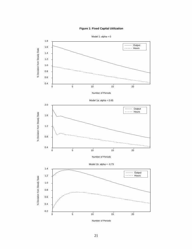
other yt = !ht, for all t. The top panel of Figure 1 illustrates that a temporary one-percent

rise in the technology shock leads to increases in ht and yt on impact, and then both variables

return monotonically towards the steady state while maintaining their (linearly) deterministic

relationship. This means that labor hours are perfectly correlated with GDP over the business

cycle, i.e., corr(ht, yt) = 1.

On the other hand, although Model 1 correctly predicts that the ratios of trade balance

and current account to output are countercyclical variables, it overstates the magnitude of

their negative comovements. This result is caused by the high degree of serial correlation

in the process that drives the productivity disturbance (� = 0:94436).10 If a less persistent

technology shock is adopted, as in Mendoza (1991) and Schmitt-Grohé and Uribe (2003), then

Model 1�s predictions of these international correlation coe¢ cients will be more quantitatively

in line with the Canadian data.

In Models 1a and 1b, the household�s preferences (2) include current and previous quantities

of labor supply that are postulated to be substitutes (� = 0:65) and complements (� = �0:73),

respectively. It turns out that both models perform no worse than the above baseline con�gura-

tion at matching the observed contemporaneous correlations with GDP, whereas incorporating

labor persistence into the analysis signi�cantly improves these models�predictions of the se-

rial correlations in key macroeconomic aggregates. In particular, as opposed to Model 1, the

autocorrelations in output, investment and hours worked are not statistically di¤erent from

the observed moments at the 5% level of signi�cance.

9 It follows that the correlation between output and average labor productivity (or the real wage rate in adecentralized equilibrium) is also equal to 1.10See Mendoza (1991, p. 807) for this point.

11

Moreover, under the same driving process for generating aggregate �uctuations, allowing

for intertemporal substitution (or the fatigue e¤ects) raises the elasticity of labor supply with

respect to changes in its marginal productivity. As a result, in contrast to Model 1, the stan-

dard deviation of hours worked is not statistically di¤erent from its empirical counterpart at

the 5% level. However, output volatility in Model 1a, while higher than that in Model 1,

remains slightly lower than what the Canadian economy displays. On the contrary, intertem-

poral complementarity (or internal habit formation) in labor inputs within Model 1b dampens

the cyclical e¤ects of technology shocks because agents are now reluctant to adjust their work

e¤ort. This feature thus leads to less variable hours worked and GDP in comparison with the

benchmark Model 1.

Next, since the household�s period-t labor supply decision takes into account its expected

in�uence on future utilities, output and employment are no longer perfectly correlated in

Models 1a and 1b. When either model is subject to a one-time positive innovation to the

production technology, the contemporaneous level of work e¤ort rises because of an outward

shift of the labor demand curve, which in turn raises the current output as well. However,

the dynamic responses after the impact period are quite di¤erent. In particular, the middle

panel of Figure 1 shows that compared to Model 1, intertemporal substitutability in Model 1a

generates higher increases in hours worked and output at the initial period. Furthermore, the

household�s substituting work e¤ort across periods leads to very similar oscillatory dynamics

of ht and yt between t = 0 and t = 3 before they fall back gradually to the steady state. As a

result, labor hours are strongly procyclical with corr(ht, yt) = 0:99, which is still statistically

too high vis-á-vis the Canadian data.

By contrast, due to the presence of habit persistence, the bottom panel of Figure 1 shows

that the initial responses of hours worked and output to a transient technology shock are

smaller in Model 1b than those in Model 1. Intertemporal complementarity also leads to a

sluggish movement in the household�s labor supply decision over di¤erent periods. It follows

that ht and yt continue to rise after the impact period in spite of a decreasing marginal

productivity of labor, thereby generating hump-shaped impulse response functions. Moreover,

the subsequent adjustment paths of employment and output are not closely synchronized in

that yt peaks at t = 4 whereas ht reaches its maximum two periods later, indicating that labor

hours now become a lagging variable of the business cycle. This results in a lower correlation

coe¢ cient between GDP and hours worked within Model 1b (= 0:92) that is remarkably

12

close to the Canadian economy in which corr(ht, yt) = 0:91. Notice that this particular

simulated moment is not statistically di¤erent from its empirical counterpart at the 5% level

of signi�cance.

3.3 Variable Capital Utilization

The second half of Table 1 presents our simulation results under variable capital utilization.

To understand the macroeconomic e¤ects of changing capital utilization, substituting (9) and

(12) into (6) yields the following reduced-form social technology as a function of capital and

labor inputs:

yt =

��

��

� ����

z�

���t k

�(��1)���

t h�(1��)���

t ; (20)

where �(��1)��� < 1 to rule out the possibility of sustained endogenous growth. Compared to the

production function (6) with �xed capital utilization, (20) exhibits a larger equilibrium elastic-

ity of output with respect to both the technology shock zt and labor hours ht. This implies that

varying capital utilization will amplify the quantitative e¤ects of productivity disturbances be-

cause it enriches the model�s endogenous propagation mechanism by providing an additional

margin to change output. As a result, even with a smoother driving process (�" is 13:36%

smaller), all variables in Models 2, 2a and 2b display substantially higher standard deviations

than their Model 1�s counterparts. In addition, since the persistence parameter of produc-

tivity disturbances � remains virtually unchanged, incorporating variable capital utilization

does not signi�cantly in�uence the model�s predictions of autocorrelations, contemporaneous

correlations with output and the savings-investment comovement.

As in Model 1, the no-labor-persistence Models 2 continues to show a counterfactual per-

fectly positive correlation between ht and yt, and statistically lower serial correlations in GDP

and hours worked than those observed in the data. On the other hand, Model 2a (with

intertemporal substitutability) �overshoots� the variabilities of output, consumption and in-

vestment, and underpredicts the autocorrelations in GDP and labor hours. By contrast,

Model 2b with habit formation in labor exhibits a statistically close match with the observed

volatilities of output, investment and the trade-balance-to-output ratio (at the 5% level of

signi�cance) and consumption (at the 1% level of signi�cance). However, the standard de-

viation of hours worked is statistically lower than the actual data because of the sluggish

movements in employment caused by the intertemporal complementarity in work e¤ort. In

13

terms of serial correlations, Model 2b successfully matches the persistence of GDP, investment,

labor hours, and the ratios of trade balance and current account to output at the 5% level,

and of consumption at the 1% level.

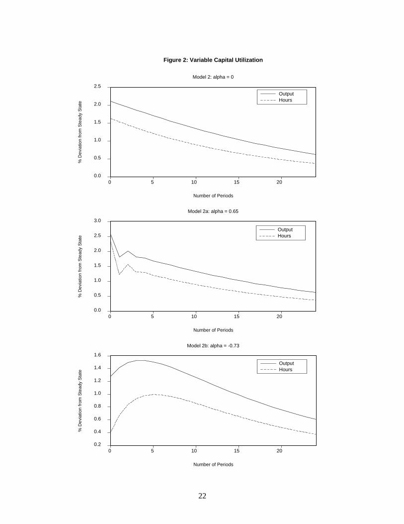
Figure 2 plots the impulse response functions for the three speci�cations with endogenous

capital utilization. In comparison with Figure 1, the initial responses of hours worked and

GDP to a transitory positive technology shock are stronger because of a larger equilibrium

output elasticity. Moreover, higher work e¤ort leads to more intensive utilization of capital,

which in turn contributes to a further immediate rise in output. In sum, varying capital

utilization strengthens the expansionary e¤ects of a temporary productivity disturbance at

the impact period. However, the ensuing dynamic responses of ht and yt in Models 2, 2a, and

2b are qualitatively identical to those in their �xed-utilization counterparts. If follows that

the correlation coe¢ cient between detrended output and labor hours is not a¤ected by the

addition of variable capital utilization alone. In particular, as in Model 1b, this correlation in

Model 2b continues to be statistically not di¤erent from its empirical counterpart at the 5%

level of signi�cance. Moreover, Model 2b moves the contemporaneous correlations between

output and the ratios of trade balance and current account to GDP in the right direction.

3.4 Sensitivity Analysis

So far, our analysis has shown that Model 2b, which is a small open, technology-shock driven

one-sector real business cycle model with variable capital utilization and internal habit forma-

tion in labor hours, is able to account for the main empirical regularities of Canada�s aggregate

�uctuations after 1981. Since the labor-persistence parameter � (= �0:73) is not calibrated

from the Canadian data, Table 2 presents simulation results and the corresponding statisti-

cal signi�cances under alternative degrees of intertemporal complementarity in work e¤ort.

It turns out that most of the autocorrelations, contemporaneous correlations with GDP and

the savings-investment comovement are quantitatively and statistically robust to variations of

�. However, when the absolute value of � rises, agents are less willing to adjust their labor

supplies across successive time periods. As a result, the volatilities of hours worked, output,

consumption and investment are all negatively related to the strength of intertemporal com-

plementarity in labor. In addition, slower changes in work e¤ort lead to a weaker comovement

between GDP and employment over the business cycle, i.e., @ corr(ht;yt)@j�j < 0.

14

4 Conclusion

Previous studies have found that it is di¢ cult to account for some of Canada�s real business-

cycle characteristics in a canonical dynamic small open economy model driven by technology

shocks. Speci�cally, in Mendoza�s (1991) formulation with a time separable utility function,

zero elasticity of intertemporal substitution in work e¤ort leads to a counterfactual perfectly

positive correlation between GDP and hours worked. Moreover, due to a weak internal prop-

agation mechanism, the volatilities and persistence of several model-generated time series

are statistically lower than those observed in the Canadian data. In this paper, we show

that adding intertemporally nonseparable labor supply and variable capital utilization to the

Mendoza economy can overcome these shortcomings. Under a time nonseparable preference

formulation, the household�s period-t labor supply decision also depends on previous and fu-

ture quantities of hours worked, hence GDP and employment are no longer perfectly correlated

over the business cycle. On the other hand, varying capital utilization enhances the cyclical

e¤ects of productivity disturbances because it provides an additional channel to change out-

put. Overall, our analysis shows that incorporating intertemporal complementarity in labor

hours and endogenous capital utilization into Mendoza�s dynamic, small open economy model

can better explain the quantitative business cycle properties of real macroeconomic variables

in the post-1981 Canadian economy.

Although our model provides an improved �t with the Canadian business cycle along sev-

eral important dimensions, it nevertheless exaggerates the procyclical nature of consumption

and investment. To address this inconsistency, it would be worthwhile to incorporate other

sources of driving uncertainties, such as preference shocks (Baxter and King, 1991) or terms-

of-trade shocks (Bergin and She¤rin, 2000), into the analysis.11 Moreover, Laxton and Pesenti

(2003) and Letendre (2004), among others, have made a case for the introduction of habit

formation in consumption with reasonable success for small open economies. Hence, it would

be interesting to study the cyclical e¤ects of habit formation in consumption as well as in labor

hours within a dynamic, small open real business cycle model. Finally, it would be valuable

to examine alternative preference speci�cations, e.g. the recursive utility framework as in

Lettau and Uhlig (2000) and Tallarini (2000). This will allow us to investigate the robustness

11Mendoza (1991), Correia, Neves and Rebelo (1995), and Letendre (2004), among others, have shown thatadding shocks to government spending and/or the world interest rate does not improve the overall �t of theclass of models that we have examined in this paper.

15

of our results, and further identify model features and parameters that a¤ect the aggregate

�uctuations in a small open economy like Canada. We plan to pursue these research projects

in the future.

16

References[1] Baxter, Marianne and Robert G. King, �Productive Externalities and Business Cycles,�

Institute for Empirical Macroeconomics at Federal Reserve Bank of Minneapolis, Discus-sion Paper 53, November 1991.

[2] Bergin, Paul R. and Steven M. She¤rin, �Interest Rates, Exchange Rates and the PresentValue Models of the Current Account,�Economic Journal 110(2000), 535-558.

[3] Burnside, C.A., M.S. Eichenbaum and S. Rebelo, �Labor Hoarding and the BusinessCycle,�Journal of Political Economy 101(1993), 245-273.

[4] Burnside, C.A. and M.S. Eichenbaum, �Factor-Hoarding and the Propagation of Business-Cycle Shocks,�American Economic Review 86(1996), 1154-1174.

[5] Campbell, J.Y., �Inspecting the Mechanism: An Analytical Approach to the StochasticGrowth Model,�Journal of Monetary Economics 33(1994), 463�504.

[6] Correia, I., J.C. Neves and S.T. Rebelo, �Business Cycles in a Small Open Economy,�European Economic Review 39(1995), 1089-1113.

[7] Eichenbaum, M.S., L.P. Hansen and K.J. Singleton, �A Time Series Analysis of Represen-tative Agent Models of Consumption and Leisure Choice Under Uncertainty,�QuarterlyJournal of Economics 103(1988), 51-78.

[8] Greenwood, J., Z. Hercowitz, and G.W. Hu¤man, �Investment, Capacity Utilization, andthe Real Business Cycle, American Economic Review 78(1988), 402-417.

[9] Gregory, A.W. and G.W. Smith, �Calibration as Testing: Inference in Simulated Macro-economic Models,�Journal of Business & Economic Statistics 9(1991), 297-303.

[10] Hotz, V.J., F.E. Kydland and G.L. Sedlacek, �Intertemporal Preferences and Labor Sup-ply,�Econometrica 56(1988), 335-360.

[11] Kydland, F.E. and E. Prescott, �Time to Build and Aggregate Fluctuations�, Economet-rica, 50(1982), 1345-1370.

[12] Laxton, Douglas and Paolo Pesenti, �Monetary Rules for Small, Open, EmergingEconomies,�Journal of Monetary Economics 50(2003), 1109-1146.

[13] Letendre, M.-A., �Capital Utilization and Habit Formation in a Small Open Economy,�Canadian Journal of Economics 37(2004), 721-741.

[14] Lettau, M. and H. Uhlig, �Can Habit Formation be Reconciled with Business CycleFacts?� Review of Economic Dynamics, 3(2000), 79-99.

[15] Mendoza, E.G., �Real Business Cycles in a Small Open Economy,�American EconomicReview 81(1991), 797-818.

[16] Schmitt-Grohé, S. and M. Uribe, �Closing Small Open Economy Models,� Journal ofInternational Economics 61(2003), 163-185.

[17] Tallarini, Thomas D. Jr., �Risk-Sensitive Real Business Cycles,� Journal of MonetaryEconomics 45(2000), 507-532.

[18] Uhlig, H., �A Toolkit for Analyzing Nonlinear Dynamic Stochastic Models,� in Compu-tational Methods for the Study of Dynamic Economies, edited by R. Maromon and A.Scott, Oxford: Oxford University Press, 1999, 30-61.

17

[19] Uzawa, H., �Time Preference, the Consumption Function, and Optimum Asset Holdings,�in Value, Capital, and Growth: Papers in Honour of Sir John Hicks, edited by J.N. Wolfe,Edinburgh: Edinburgh University Press, 1968, 485-504.

[20] Wen, Y., �Can A Real Business Cycle Model Pass the Watson Test?�Journal of MonetaryEconomics 42(1998), 185-203.

18

Table 1: Observed and Simulated Second Moments

I. Fixed Capital Utilization II. Variable Capital UtilizationData Model 1 Model 1a Model 1b Model 2 Model 2a Model 2b

� = 0 � = 0:65 � = �0:73 � = 0 � = 0:65 � = �0:73Volatilities:

std(yt) 1.72 1.39�� 1.67�� 1.37�� 2.27� 2.39 1.71��

std(ct) 0.93 0.92�� 1.07�� 1.09�� 1.36 1.37yy 1.22�

std({t) 5.13 4.12yy 4.96��yy 4.08yy 6.74�yy 7.11yy 5.01��yy

std(ht) 1.25 0.82 1.02�� 0.66 1.34�� 1.50� 0.81

std( tbtyt ) 0.87 0.31 0.34 0.54�yy 0.72��yy 0.74��yy 0.84��yy

std( catyt ) 0.29 0.30�� 0.34��y 0.54� 0.71 0.74 0.83

Serial Correlations:

corr(yt, yt�1) 0.91 0.70 0.76 0.85�� 0.79 0.68 0.86��

corr(ct, ct�1) 0.83 0.70� 0.85�� 0.77� 0.78� 0.83�� 0.77�

corr({t, {t�1) 0.88 0.68 0.79�� 0.80�� 0.78� 0.75� 0.82��

corr(ht, ht�1) 0.92 0.70 0.68 0.94�� 0.79 0.57 0.94��

corr( tbtyt ,tbt�1yt�1

) 0.67 0.69�� 0.76�� 0.71�� 0.78�� 0.77�� 0.73��

corr( catyt ,cat�1yt�1

) 0.68 0.69�� 0.78�� 0.73�� 0.78�� 0.76�� 0.73��

Contemporaneous Correlations with Output :

corr(ct, yt) 0.80 0.99 0.98 0.97 0.99 0.97 0.97

corr({t, yt) 0.77 0.98 0.97 0.94 0.98 0.98 0.96

corr(ht, yt) 0.91 1.00 0.99 0.92�� 1.00 0.99 0.93��

corr( tbtyt , yt) -0.29 -0.89 -0.69 -0.55 -0.85 -0.76 -0.63

corr( catyt , yt) -0.26 -0.85 -0.65 -0.54 -0.82 -0.71 -0.60

Savings-Investment Correlation:

0.77 0.63�� 0.66�� 0.35�� 0.80�� 0.80�� 0.54

Notes: The superscripts �� and � show that an observed moment is not statisticallydi¤erent from its simulated counterpart at the 5% and 1% levels of signi�cance,respectively. The subscripts yy and y show that the observed relative standarddeviation of a variable to that of output is not statistically di¤erent from itssimulated counterpart at the 5% and 1% levels of signi�cance, respectively.

19

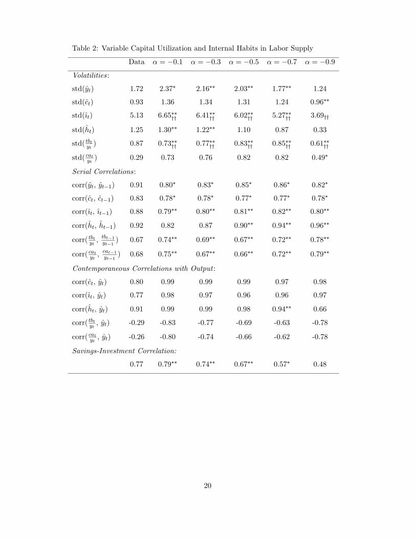
Table 2: Variable Capital Utilization and Internal Habits in Labor Supply

Data � = �0:1 � = �0:3 � = �0:5 � = �0:7 � = �0:9

Volatilities:

std(yt) 1.72 2.37� 2.16�� 2.03�� 1.77�� 1.24

std(ct) 0.93 1.36 1.34 1.31 1.24 0.96��

std({t) 5.13 6.65��yy 6.41��yy 6.02��yy 5.27��yy 3.69yy

std(ht) 1.25 1.30�� 1.22�� 1.10 0.87 0.33

std( tbtyt ) 0.87 0.73��yy 0.77��yy 0.83��yy 0.85��yy 0.61��yy

std( catyt ) 0.29 0.73 0.76 0.82 0.82 0.49�

Serial Correlations:

corr(yt, yt�1) 0.91 0.80� 0.83� 0.85� 0.86� 0.82�

corr(ct, ct�1) 0.83 0.78� 0.78� 0.77� 0.77� 0.78�

corr({t, {t�1) 0.88 0.79�� 0.80�� 0.81�� 0.82�� 0.80��

corr(ht, ht�1) 0.92 0.82 0.87 0.90�� 0.94�� 0.96��

corr( tbtyt ,tbt�1yt�1

) 0.67 0.74�� 0.69�� 0.67�� 0.72�� 0.78��

corr( catyt ,cat�1yt�1

) 0.68 0.75�� 0.67�� 0.66�� 0.72�� 0.79��

Contemporaneous Correlations with Output :

corr(ct, yt) 0.80 0.99 0.99 0.99 0.97 0.98

corr({t, yt) 0.77 0.98 0.97 0.96 0.96 0.97

corr(ht, yt) 0.91 0.99 0.99 0.98 0.94�� 0.66

corr( tbtyt , yt) -0.29 -0.83 -0.77 -0.69 -0.63 -0.78

corr( catyt , yt) -0.26 -0.80 -0.74 -0.66 -0.62 -0.78

Savings-Investment Correlation:

0.77 0.79�� 0.74�� 0.67�� 0.57� 0.48

20

0.4

0.6

0.8

1.0

1.2

1.4

1.6

1.8

0 5 10 15 20

Number of Periods

OutputHours

% D

evia

tion

from

Ste

ady

Sta

teModel 1: alpha = 0

0.4

0.8

1.2

1.6

2.0

0 5 10 15 20

Number of Periods

OutputHours

% D

evia

tion

from

Ste

ady

Sta

te

Model 1a: alpha = 0.65

0.2

0.4

0.6

0.8

1.0

1.2

1.4

0 5 10 15 20

Number of Periods

OutputHours

% D

evia

tion

from

Ste

ady

Sta

te

Model 1b: alpha = -0.73

Figure 1: Fixed Capital Utilization

21

0.0

0.5

1.0

1.5

2.0

2.5

0 5 10 15 20

Number of Periods

OutputHours

% D

evia

tion

from

Ste

ady

Sta

teModel 2: alpha = 0

0.0

0.5

1.0

1.5

2.0

2.5

3.0

0 5 10 15 20

Number of Periods

OutputHours

% D

evia

tion

from

Ste

ady

Sta

te

Model 2a: alpha = 0.65

0.2

0.4

0.6

0.8

1.0

1.2

1.4

1.6

0 5 10 15 20

Number of Periods

OutputHours

% D

evia

tion

from

Ste

ady

Sta

te

Model 2b: alpha = -0.73

Figure 2: Variable Capital Utilization

22