Business Cycles in Small, Open Economies: Evidence from ...€¦ · Bank of Canada Staff Working...

Bank of Canada staff working papers provide a forum for staff to publish work-in-progress research independently from the Bank’s Governing Council. This research may support or challenge prevailing policy orthodoxy. Therefore, the views expressed in this paper are solely those of the authors and may differ from official Bank of Canada views. No responsibility for them should be attributed to the Bank.

www.bank-banque-canada.ca

Staff Working Paper/Document de travail du personnel 2016-48

Business Cycles in Small, Open Economies: Evidence from Panel Data Between 1900 and 2013

by Wataru Miyamoto and Thuy Lan Nguyen

2

Bank of Canada Staff Working Paper 2016-48

November 2016

Business Cycles in Small, Open Economies: Evidence from Panel Data Between 1900 and 2013

by

Wataru Miyamoto1 and Thuy Lan Nguyen2

1Canadian Economic Analysis Department Bank of Canada

Ottawa, Ontario, Canada K1A 0G9 [email protected]

2Santa Clara University Santa Clara, California

[email protected]

ISSN 1701-9397 © 2016 Bank of Canada

mailto:[email protected]

mailto:[email protected]

i

Acknowledgements

We thank Emi Nakamura, Serena Ng, Stephanie Schmitt-Grohé, Jón Steinsson and Martín Uribe for their invaluable advice. We also thank two anonymous referees, Jonathan Dingel, Andres Fernandez, Alex Field, Pablo Guerron-Quintana, Chris Otrok and seminar participants at the 2012 Midwest Macroeconomic Meeting, Econometric Society European Meeting and Columbia Economic Fluctuation and Monetary Colloquia for their input. We also thank Chris Otrok for his help with the dynamic factor approach, and Leandro Prados de la Escosura, Alpay Filitztekin, Ola Gryten, Gudmundur Jonsson, Jari Kauppila, Pedro Lain, Eduardo Moron, Bruno Seminario and Jose Ursua for providing us with the data.

ii

Abstract

Using a novel data set for 17 countries dating from 1900 to 2013, we characterize business cycles in both small developed and developing countries in a model with financial frictions and a common shock structure. We estimate the model jointly for these 17 countries using Bayesian methods. We find that financial frictions are an important feature for not only developing countries but also small developed countries. Furthermore, business cycles in both groups of countries are marked with trend productivity shocks. Common disturbances explain one-third of the fluctuations in small, open economies (both developed and developing), especially during important worldwide phenomena.

Bank topics: Business fluctuations and cycles; Economic models; International topics JEL classification: F41; F44; E13; E32

Résumé

Grâce à un nouvel ensemble de données sur 17 pays couvrant la période de 1900 à 2013, nous caractérisons les cycles économiques de petits pays développés et de pays en développement dans un modèle doté de frictions financières et d’une structure de chocs commune. Nous estimons le modèle pour les 17 pays collectivement en recourant à des méthodes bayésiennes. Nous constatons que les frictions financières constituent une caractéristique importante non seulement des pays en développement, mais aussi des petits pays développés. Par ailleurs, les cycles économiques des deux groupes de pays sont marqués par des chocs de productivité tendancielle. Les perturbations communes expliquent le tiers des fluctuations dans les petites économies ouvertes (qu’il s’agisse de pays développés ou de pays en développement), en particulier durant des phénomènes mondiaux importants.

Sujets : Cycles et fluctuations économiques; Modèles économiques; Questions internationales Codes JEL : F41; F44; E13; E32

Non-Technical Summary Motivation and Question

Previous studies have pointed out two key differences in the business cycles of emerging economies and advanced economies: the former exhibit more volatility in consumption relative to output and more countercyclical trade balance. Two views try to explain these features. Aguiar and Gopinath (2006) argue that these differences can be well explained by shocks to trend productivity that may reflect changes in economic policies and market failure. In contrast, Garcia-Cicco et al. (2010) show that financial frictions are better suited to capture the different dynamics in business cycles. Given the contrasting views of these studies, which use relatively few emerging countries, we try to answer the following questions. First, in the data, what are the key features of business cycles in developing countries, once we significantly extend the number of emerging countries and the time horizon in the analysis? Second, do financial frictions play a more prominent role than trend productivity shocks, once we employ a more general framework than those used in previous studies? Third, are business cycles in small developed countries different from those in developing countries?

Methodology

First, we document the main business cycles statistics for both small developed and developing countries using a novel and rich data set covering macroeconomic variables for 17 countries between 1900 and 2013. Then, we build a small open economy real business cycle model with reduced-form financial frictions and trend productivity shocks, augmented with common shocks that affect all countries at the same time. Our model nests those developed by Aguiar and Gopinath (2006) and Garcia-Cicco et al. (2010), which allows us to quantify the relative importance of their hypotheses. Finally, we estimate the model using Bayesian methods jointly for the 17 countries in our data set.

Key Contributions First, we show that financial frictions are an important feature of business cycles in both small developed and developing countries. Second, contrary to previous literature, we find that trend productivity shocks play a sizable role in driving business cycles in both small developed and developing countries. However, the natures of trend productivity shocks are different: while common trend shocks are more important than country-specific shocks in developed economies, it is the opposite in developing countries. Third, common disturbances across countries are important drivers of business cycles. Future Research

Our results suggest that future research should investigate the transmission mechanism of shocks and the general equilibrium effects from large countries to small open economy countries through international trade of both goods and financial assets.

1 Introduction

Recent studies have examined whether economic fluctuations in developing countries are described

well by a frictionless real business cycle (RBC) model with shocks to trend productivity. Using

data for Mexico, Aguiar and Gopinath (2007) argue that a frictionless RBC model with trend

productivity shocks goes a long way in explaining business cycles in developing countries, as trend

productivity shocks can capture frequent regime switches in economic policies and market failures,

which are important for these countries. At the same time, Garcia-Cicco et al. (2010) show that an

RBC model with a reduced-form financial friction describes the data for Argentina better than a

frictionless model, and that it predicts the negligible role of trend productivity shocks in aggregate

fluctuations. Given these contrasting conclusions coming from studies with relatively few countries,

several questions on the nature of the business cycle in small open economies remain. First, what

are the important features of economic fluctuations in developing countries in general? Do trend

productivity shocks have a negligible role, while financial frictions are at the front and center?

Second, are business cycles in small developed countries any different from those in developing

countries over the long horizon?

This paper answers these questions in a unified framework of a structural model for small open

economies and provides new evidence on the characteristics of business cycles using a novel panel

data set covering over 100 years of data for 17 small developed and developing countries. Our

structural model is a small open economy RBC model with financial frictions and common shocks.

The financial friction feature of the model provides us with a framework to analyze whether a

frictionless RBC model with trend productivity shocks or a model with financial frictions can better

describe key features of business cycles in small open economies over the long horizon. Importantly,

unlike previous papers in the literature, we introduce a common shock structure into the model

to capture the possibility that these countries are subject to some common outside shocks and to

better utilize the information from the panel data of many countries. More specifically, our model

includes 17 small open economies, each of which faces a reduced-form financial friction modeled

as an endogenous interest rate premium that responds to both the level of debt-to-output ratio

and expected future productivity. The model economy is buffeted by five types of shocks including

trend and stationary productivity shocks and country premium shocks, each of which has two

components: a world common shock that affects all countries at the same time, and a country-

specific shock. These common shocks are what connect these small open economies and can be

1

interpreted as outside shocks.

To facilitate our analysis, we estimate the model using a new data set covering 17 developing and

developed small open economies between 1900 and 2013. Compared with previous studies, our data

set includes many more countries over a much longer horizon, providing us with new evidence on the

important features of business cycles in both small developed and developing economies, which has

been limited in both sample countries and sample periods. Furthermore, given the panel structure

of the data set, we pool all available information and estimate the model jointly for these countries.

Therefore, we obtain efficiency gain in estimating key parameters and can identify structural shocks

more accurately. Even though long data series may contain measurement errors, the fact that these

series contain several business cycles makes them suitable for our purpose, to characterize observed

business cycles and identify structural parameters in the model, especially those related to the

trend productivity shock process. Furthermore, as we pool data in our estimation, the problem

with measurement errors is less pronounced, to the extent that these measurement errors are

independent across countries.

Our joint estimation for all 17 countries using Bayesian methods indicates that financial frictions

are an important feature of business cycles in both small developed and developing countries.

In other words, a frictionless RBC model is not supported by the data. In fact, all 17 small

open economies in our sample face non-zero financial frictions, although the estimated degree of

financial frictions varies across countries. Our estimation results suggest that while it is difficult for

households to smooth their consumption by borrowing internationally, their borrowing constraint

is also relaxed when their expected future productivity is high.

An important finding of our analysis is that trend productivity shocks play a sizable role in both

small developed and developing countries. In particular, trend productivity shocks explain about

one-third of output fluctuations in both small developed and developing countries, on average.

This result is substantially different from previous studies on the importance of trend productivity

shocks in emerging economies, such as Garcia-Cicco et al. (2010), who find that in an estimated

model with financial frictions for Argentina, trend shocks are a negligible source of business cycles.

Our estimation suggests that Argentina is a particular case, since in other countries such as Taiwan

and Portugal, trend productivity shocks are large and significant even though these countries face

substantial financial frictions. The contribution of trend productivity shocks is, on average, much

larger than that in Argentina. Nevertheless, on average, trend plays a less significant role than

stressed in Aguiar and Gopinath (2007), who examine Mexico after 1980. This result highlights

2

the importance of using information from many countries over the long horizon to understand the

nature of business cycles in small open economies.

Although trend productivity shocks explain a significant fraction of business cycle fluctuations

in both developed and developing countries, the natures of trend productivity shocks differ be-

tween these two groups of countries. When we decompose the importance of trend and stationary

shocks into common and country-specific components, our estimation finds that while important

trend shocks in small developed countries are common, country-specific trend shocks are much

more dominant in developing countries. We interpret this result as follows: Developed countries

are generally closer to the world productivity frontier, so they are more prone to common trend

productivity shocks. However, developing countries are subject to various domestic policy and

structural reforms, so the trend productivity shocks that are important for them are not common

but country-specific.

Another finding in our paper is that common disturbances across countries are an important

driving force of business cycle fluctuations in small open economies. These common shocks capture

worldwide phenomena in the last 100 years such as the Great Depression, the two World Wars, the

two oil price shocks and the Great Recession. During these episodes, output in all these countries

dropped at the same time. Therefore, the estimation attributes a substantial fraction of business

cycle fluctuations in both developed and developing countries to these common disturbances. In

particular, all types of common shocks account for roughly 28% of output fluctuations at an annual

frequency over the last 100 years. Furthermore, the extracted world common shocks are highly

correlated with U.S. output over time. For example, in the 2008–09 recession, output in Canada

and Mexico, which have strong ties with the U.S., declined significantly due to common shocks.

These results suggest that the identified common shocks include the general equilibrium effects

of shocks from large countries, such as the U.S., to 17 small open economies through financial

and trade linkages.1 Finally, we document that several sources of common shocks contribute to

the fluctuations of macroeconomic variables, including common trend and stationary productivity

shocks, as well as common premium shocks.

To examine whether business cycles have changed substantially over the last 100 years, we

estimate the model for the two subsample periods before and after 1950. We find that the esti-

1It is possible that our common shocks include the shocks originating from one of the 17 countries transmittingto the rest of the countries in the sample, which can overstate the importance of common shocks. However, thisbias may be small. The reason is that since our sample includes 17 small open economies, shocks originating fromArgentina or Canada are unlikely to affect other countries such as Taiwan or India. In other words, data from smallopen economies can help to avoid some of the internal propagation among countries in the group.

3

mated parameters of the model, including those related to the financial friction, change over time,

consistent with the fact that some of the second moments, such as volatilities in the data, are

different across the two subsample periods. However, the main findings of our paper are robust:

trend productivity shocks as well as common shocks play a sizable role in business cycles in these

countries, and financial frictions are still an important feature for small open economies.

Although the identification in Bayesian estimation relies on all the information and moments in

the data, our analysis suggests that the behaviors of trade balance, as well as output and consump-

tion growth rates, help to pin down the importance of trend and productivity shocks. In particular,

in a frictionless RBC model, although trend productivity shocks can lead to countercyclical trade

balance and the excess volatility of consumption, trend productivity shocks lead to a near random-

walk trade balance, as discussed in Garcia-Cicco et al. (2010). Therefore, observing trade balance

is important in identifying whether a frictionless RBC model is adequate in explaining business

cycles in small open economies or whether financial frictions are an important feature for these

economies. Furthermore, observing output and consumption growth rates over the long horizon

also helps to identify the persistence of productivity shocks, and the estimation to distinguish trend

and stationary productivity shocks. We identify the common components of these shocks through

both contemporaneous and dynamic correlations across all country pairs. In the model, since each

country is a small open economy, there is no correlation across countries without common shocks.

Therefore, the estimation attributes the comovements across all countries to world common shocks,

and the fluctuations independent of other countries to country-specific shocks. This identification

implies that common shocks tend to be more important for countries that are more correlated with

the rest of the countries in the sample, which is consistent with our findings.

Related Literature Our paper is related to several strands of the macroeconomics literature.

First, we contribute to a large literature in the small open economy business cycle studies, starting

with Mendoza (1991), by providing new evidence on the role of trend shocks and financial frictions

in a large number of countries.2 These papers often focus on only a few countries, such as Argentina

and Mexico, and use short time series. Although Garcia-Cicco et al. (2010) use 100 years of data,

their sample countries are also limited to Argentina and Mexico.3 We complement these papers

2A number of papers including Neumeyer and Perri (2005), Uribe and Yue (2006), Aguiar and Gopinath (2007),Chang and Fernandez (2013), Alvarez-Parra et al. (2013), Fernandez-Villaverde et al. (2011), and Fernandez andGulan (2015) have highlighted the role of interest rate, the changes in interest rate volatility, trend shocks andfinancial frictions in business cycles in emerging economies.

3Nakamura et al. (2014) estimate a trend component using consumption data for 16 developed countries spanning100 years in a long run risk model.

4

along several dimensions. We estimate trend shocks using a new data set that covers many more

countries, spanning over a century. Our finding about the importance of trend shocks in these

countries suggests that trend shocks are neither dominant nor negligible as earlier works with

only a few countries have found. Furthermore, we also highlight the role of financial frictions in

developing countries, unlike Naoussi and Tripier (2013), who use shorter data for 82 countries but

restrict their attention to a frictionless model with trend shocks. This finding resonates with recent

work by Akinci (2014) and Fernandez and Gulan (2015), who quantify the role of financial frictions

in a micro-founded financial friction model using recent data. Finally, an important difference

between our papers and earlier work in this literature is that we exploit the information from the

long panel data to examine the common components of trend shocks and how financial frictions

have changed over time for these small open economies.4

Our paper also provides new evidence of the role of common shocks to the existing literature on

world business cycles. Structural studies such as Glick and Rogoff (1995) and Gregory and Head

(1999) distinguish the effects of common and country-specific shocks, but do not estimate the model.

Therefore, they do not address our questions on business cycles in small open economies. A recent

work by Guerron-Quintana (2013) estimates the role of common shocks in small developed countries

using quarterly data from 1980. Our paper, instead, focuses on business cycle characteristics for

not only small developed countries but also emerging countries over 100 years. Besides, our model

features an endogenous interest rate premium to proxy for the reduced-form financial friction in

these countries, as well as a flexible common shock structure to capture the observed comovements

in the data. Both differences matter for the results, as they affect identification and fitness of the

model.

We also speak to a large literature on understanding world business cycles using reduced-form

dynamic factor models (DFM) such as Kose et al. (2003, 2012). An important contribution of

our paper is that we identify several types of structural common shocks and their propagation

mechanism, which is difficult in a standard DFM approach. If we used standard DFM estimation

in the international business cycle literature, which typically assumes one type of common factor,

we would estimate a much more modest role of common shocks—about half of the result in the

structural estimation. We demonstrate this difference between structural and DFM methods by

showing that DFM estimates a much lower importance of common shocks when the data-generating

4A few other papers such as Kose (2002) and recently Fernandez et al. (2015) explore the role of commodity pricesin driving business cycles in small open economies. We do not specify the commodity prices in our model, but wecan interpret that some of the shocks we identify come from the fluctuations in commodity prices.

5

process has more than one type of common shock.5

The rest of the paper is organized as follows: Section 2 documents the main business cycle

statistics of small developed and developing countries between 1900 and 2013. Section 3 describes

the baseline model. We explain the estimation method and the identification issues in Section 4.

We discuss the role of financial frictions in Section 5. We present our main findings on the relative

role of trend and stationary shocks and the nature of these shocks in Section 6 and 7. Section 8

analyzes the role of common shocks in small open economies. Section 9 discusses the robustness of

our findings when we look at two subsample periods in our data. Section 10 concludes.

2 Business Cycles in Small Open Economies: 1900–2013

This section documents the main business cycle statistics for small open economies using a novel

data set covering 17 countries in the last 100 years.

Our new data set includes annual growth rates of output, consumption, investment and the

trade balance-to-output ratio for 17 small developed and developing countries between 1900 and

2013. Output, consumption and investment are deflated by the GDP deflator and in per capita

terms. We start our data set with countries that have output and consumption data in Barro

and Ursua (2010). We exclude large countries such as the United States, Japan, Germany, France

and the United Kingdom, which represented more than 2% of the world’s GDP in the year 2000.

We then collect data on investment and trade balance for the remaining countries from various

sources, such as national statistics offices and economic history publications.6 Since the data for

many countries start after World War II and the motivation of the paper is to use long data series

to identify trend shocks, we choose only countries with at least 89 years of data, leaving these 17

countries.7

We categorize the countries into two groups based on their present development level, similar

to Kose et al. (2012). Our classification is also consistent with that of Morgan Stanley Capital

International (MSCI), which is used in Alvarez-Parra et al. (2013).8 There are 10 developing

countries (Argentina, Brazil, Chile, Colombia, India, Mexico, Peru, Taiwan, Turkey and Venezuela)

5 Our results may be consistent with the DFM approach that identifies several common factors. However, astandard DFM estimation is not adequate to address our research questions; i.e., to understand the role of financialfrictions as well as the nature of driving forces in business cycles and the propagation mechanisms.

6Detailed data sources are listed in Appendix C.7Data availability for the countries in our data set is detailed in Appendix Table A1.8We classify a country as developed if the country was in the MSCI Developed Markets index in their classification

and as having an emerging market otherwise.

6

and seven small developed countries (Australia, Canada, Finland, Norway, Portugal, Spain, and

Sweden). This grouping helps us characterize the differences between small developed countries

and developing countries.9

2.1 Within-Country Statistics

[Insert Table 1 around here]

Whole sample: 1900–2013. Some features of our long time-span data set are similar to the facts

previously documented in shorter data series. First, business cycles in many developing countries

are characterized by a more volatile consumption growth rate than output growth rate, as shown

in column (1) and column (2) of the “Developing” panel in Table 1. This feature also holds, on

average, across small developed countries. Second, investment is the most volatile variable in every

country in the sample, as displayed in column (3) of Table 1. Third, consistent with standard

business cycle facts, consumption and investment are positively correlated with output. Lastly,

the autocorrelation of trade balance is high, as reported in column (13) of Table 1. We also find

that the trade balance autocorrelation function tapers off quickly for all countries, similar to that

reported in Garcia-Cicco et al. (2010) using shorter data.10

Our data set also exhibits several features that are different from the previously documented

facts. First, consumption volatility is higher than output volatility in small developed countries,

on average. As reported in the first two columns of Table 1, this is true for five out of seven small

developed economies. The excess volatility of consumption is in contrast with previous studies

such as Aguiar and Gopinath (2007), who find this feature prominent only for developing countries

using quarterly data after 1980, but consistent with other studies that use annual data from 1960,

such as Crucini and Chen (2011) and Rondeau (2012). Second, there is no strong pattern for

trade balance in small developed countries. Three out of seven small developed countries have a

countercyclical trade balance, as shown in column (7) of Table 1, while the other four countries

have a mildly procyclical trade balance. Thus, the average correlation of output and trade balance

across countries is only slightly positive.

9Previous literature estimates global business cycles by grouping countries based on geographical locations. Wedo not estimate such group components, because there are only one or two countries in some regions, which can be aproblem when we want to identify the regional shocks. We can identify the group components if we divide the groupbased on the levels of development in the estimation. However, some countries such as Argentina may have switchedbetween developed and developing groups over the entire 100 years, so we do not estimate the group components inthe baseline.

10We plot the autocorrelation function for all countries in Figure A2.

7

Since many small open economies have gone through substantial changes in the last 100 years,

we report the business cycle statistics in small open economies in two subperiods: between 1901 and

1950, and between 1951 and 2013. We choose the break point at 1950 to avoid some of the lasting

effects of World War II.11 Table 2a reports the second moments averaged across all countries, all

developed and developing countries in these two periods.

[Insert Table 2a Table 2b around here]

Subperiod: 1901–1950. During the first half of the 20th century, output, consumption and

investment growth rates are much more volatile in both small developed and developing countries

than in the whole sample. However, we still find that consumption is 50% more volatile than output

in all countries, and investment is three to four times more volatile than output. The correlation

between output and trade balance and the autocorrelation of all four variables are consistent with

the statistics for the whole period. For example, output comoves positively with consumption and

investment in all countries. Trade balance is countercyclical in developing countries, but acyclical

in small developed countries. Overall, the main difference between this subperiod and the whole

sample is that output, consumption and investment are substantially more volatile in this subperiod.

Subperiod: 1951–2013. One important difference between this subsample and the whole sample

is that the volatilities of output, consumption and investment are much smaller in the period

between 1951 and 2013. This pattern is true for not only small developed countries, but also

developing countries. Trade balance, on the other hand, remains as volatile as the whole sample and

the 1901–1950 period.12 Other characteristics we document in the whole sample remain the same.

For example, consumption is still, on average, more volatile than output in both developed and

developing countries. Investment is still the most volatile component. Finally, the countercylicality

of trade balance remains similar to that of the whole sample.13

11Garcia-Cicco et al. (2010) compares output volatilities before and after 1945. Romer (1999) divides the samplefor the United States into: Pre World War I (1886–1916), Inter War (1920–40), Post World War II (1948–97).

12We formally test the differences in the standard deviation of output, consumption, investment and trade balancebetween two subperiods for each country. We find that for output, we can reject the hypothesis that the standarddeviations are equal between the two subperiods for all countries, except for Argentina, Brazil, Peru and India, atthe 5% significance level. We can reject the same hypothesis for consumption and investment of all countries exceptthree. Trade balance results are mixed: we can reject the hypothesis for only nine out of 17 countries.

13In the recent period between 1980 and 2013, most of the second moments for these countries remain similar tothose of the 1950–2013 period. The main difference is that the volatilities of output and consumption in developedcountries decrease further compared with the whole period and the 1950–2013 period. Since there have been only afew business cycles since 1980 for most of these countries, which makes it difficult to reliably identify trend shocks,our robustness check does not estimate the model using this subsample, but only the 1950–2013 period data.

8

2.2 Cross-Country Statistics

[Insert Figure 1 around here]

Business cycles are correlated across these small open economies for the last 100 years. As

shown in Figure 1, which plots the output growth rates for all countries in our sample excluding

Taiwan, output growth rates move in tandem in many periods between 1900 and 2013, such as in

the Great Depression and the two World Wars.14 Besides output, consumption, investment and

trade balance are also positively correlated across countries, as reported in Table 2b, where we take

an average of the cross-country correlation across all pairs of countries.

Consistent with the international business cycle features, cross-country correlations of output

are higher than that of consumption in all pairs of countries. The average correlations of output

and consumption across developing countries are lower than those across developed countries. For

example, the correlation of output is 0.22 on average among developed countries, while it is 0.15

among developing countries. One reason for lower average cross-country correlations across devel-

oping countries is that the strength of comovement varies across pairs of countries. For example,

Venezuela and India are negatively correlated or barely correlated with other countries in the sam-

ple, while Argentina is significantly positively correlated with other countries (0.19 on average). In

fact, many developing economies in South America are substantially correlated with each other.15

The same is true for the cross-country correlations of consumption growth rates. However, the

cross country correlations of investment and trade balance are higher in developing countries than

in small developed countries.

Finally, we calculate the cross-country correlations across countries for two subperiods: 1901–

1950 and 1951–2013 as reported in Table 2b. The average correlations across countries in both

subsamples are similar to those of the whole sample. For example, output is still more correlated

across countries than consumption, and the comovement is stronger among developed countries than

developing countries, on average. One noticeable difference is that output comoves more strongly

in the 1951–2013 period among developed economies (0.34 on average) than in the first 50 years

of the sample (0.19). However, the reverse is true for developing countries: their output is slightly

more correlated in the first 50 years than in the 1951–2013 period. These strong comovements

across countries motivate our focus on the common component driving the business cycles of both

small developed and developing countries.

14Taiwan has a large drop of output growth rate in 1945. The plot for all countries is in Appendix Figure A3.15We report in Appendix Table A2 the cross-country correlation of output growth rates for each pair of countries.

9

3 The Baseline Model

This section presents the baseline model to understand the importance of financial frictions and

quantify the sources of business cycles, including trend and stationary productivity shocks and

the role of common shocks in small open economies. Our model is a small open RBC model with

two features that encompass the influential papers in the literature: Aguiar and Gopinath (2007)

(AG), Garcia-Cicco et al. (2010) (GPU) and Chang and Fernandez (2013) (CF). First, our model

includes an interest rate that responds to both the level of debt and expected productivity in

each country. The responsiveness of the interest rate to these two components is the reduced-form

financial frictions.16

Second, to exploit the information from pooling the data of 17 small open economies, we aug-

ment the shock structure to include common world shocks in addition to country-specific shocks

in all of the five structural shocks: trend and stationary productivity, preference, interest rate

premium and government spending shocks. Common shocks are the only source of comovements

across countries; i.e., there is no endogenous propagation of country-specific shocks. This assump-

tion may bias the contribution of common shocks. However, since the size of each country is small,

and unless one country is a major trading partner with many countries in the sample, it is unlikely

that a shock from one country such as Argentina can spill over to other countries in the sample.

Therefore, the bias caused by shocks propagated from larger countries within our sample may not

be substantial. Additionally, we assume that common shocks can have different effects, including

different signs on different countries, similar to Gregory and Head (1999). This assumption is to

capture the heterogeneous responses of each country to common shocks.17

We describe below the detailed model for an individual economy, j ∈ [1, N ].

A representative household maximizes the following utility function:

U = E0

∞∑t=0

βtbjtu(Cjt, hjt) (1)

where bjt is the preference shock of country j at time t, β is the subjective discount factor, Cjt

16In AG, there are no financial frictions. In GPU, financial frictions take the form of an estimated debt elasticinterest rate, while it is an estimated elasticity of the real interest rate to expected productivity in CF. We note thatCF also include working capital in their model, although the role of working capital friction turns out to be negligible,which is consistent with our results for our model with working capital.

17We keep our model as close to previous literature as possible so as to better compare the results. The model ina previous version of our paper includes variable capital utilization. The estimation results of that model are similarto the results in this paper.

10

is consumption of country j at time t, and hjt is hours worked. In the model, the period utility

function u(Cjt, hjt) is assumed to be given by:

u(Cjt, hjt) =

[Cjt − ψ 1

θXjt−1 (hjt)θ]1−σ

− 1

1− σ, (2)

where θ > 0 determines the Frisch elasticity of labor supply, which is 1θ−1 , ψ > 0 is a scale

parameter, and Xjt is the trend component in the production function to induce stationarity. This

GHH preference has been used widely in the small open economy literature (Mendoza (1991), GPU,

among others) since it can generate the countercyclical behavior of the trade balance-to-output and

avoid the case where hours fall in response to a rise in trend productivity due to wealth effect.

The representative household faces the following period-by-period budget constraint:

Djt+1

Rjt≥ Djt − Yjt + Cjt +Gjt + Ijt +

sj

2

(Kjt+1

Kjt− µjss

)2

Kjt, (3)

where Djt+1 is the stock of debts chosen at time t, and Rjt denotes the interest rate on bonds

held between period t and t+ 1, Yjt is the total output, Gjt is the government spending, which is

exogenously determined, Ijt is the total investment, sj ≥ 0 is a parameter for the capital adjustment

cost, and µjss is the steady state growth rate. Capital stock evolves according to the following law

of motion:

Kjt+1 = (1− δ )Kjt + Ijt (4)

where δ > 0 is the depreciation rate of capital.

Each economy is also subject to country premium interest rate shocks. The interest rate, Rjt,

that country j faces is then given by:

Rj,t = Rj,ss exp

[φjD

(Dj,t+1/Xj,t

yj,ss− dj,ssyj,ss

)− φjSR

(EtSRj,t+1

SRj,ss− 1

)]pmj,t,

where Rj,ss is the steady state interest rate of country j, yj,ss, SRj,ss and dj,ss are the steady state

stationary detrended output, the normalized Solow residuals and bond holding level of country j,

respectively, and pmjt is the interest rate premium shock. The parameters φjD > 0 and φjSR ≥ 0

govern the sensitivity of interest rate to debt and Solow residuals.

11

Following CF, the normalized Solow residuals SRj,t is defined as follows:

SRj,t+1 = aj,t+1

(Xj,t+1

Xj,t

)1−α,

where ajt and Xjt are the transitory and trend productivity shocks, respectively. In this specifica-

tion, the real interest rate is sensitive to both the debt-to-output level relative to its steady state

through φjD, and the productivity (Solow residuals) through φjSR. This formulation is motivated by

the sovereign default literature and small open economy business cycles literature. For example, in

Arellano (2008), the probability of default depends on both bond holdings and output; Uribe and

Yue (2006) find evidence in their vector autoregression (VAR) that the real interest rate depends

on both the level of output and trade balance-to-output ratio.18 While Neumeyer and Perri (2005)

and CF model the country interest rate to inversely depend on expected productivity as future

productivity can reduce the risk of default, GPU formulate their financial frictions as a debt-elastic

interest rate, as a higher level of debt to output leads to a higher risk of default. Since both debt

holding and productivity can, in principle, affect the real interest rate a country faces, we let the

data determine the strength of each component in affecting the interest rate by estimating both

φjD and φjSR. The higher φjD is, the more the interest rate adjusts with respect to the amount of

debt that country j holds, i.e., when debt over steady state output ratio changes by 1%, interest

rate changes by φjD%.19 Similarly, the lower φjSR is, the less the interest rate adjusts with the level

of productivity in the economy. Estimating these two parameters allows us to test whether the

frictionless RBC model (when both φs are near zero) is supported by the data, and to compare the

relative lending and borrowing costs that these countries are facing.

The representative household maximizes the expected lifetime utility, subject to the budget

constraint above and a no-Ponzi condition:

limh→∞

EtDjt+h

Πhs=0Rjs

≤ 0. (5)

The production function takes a standard Cobb–Douglas form:

Yjt = ajt (Kjt)α (Xjthjt)

1−α . (6)

18In our model, the movement of trade balance-to-output ratio is closely related to that of Dj,t.19Except for GPU, most papers in the literature, such as AG, CF and Guerron-Quintana (2013), assign φj to be

small only to induce stationarity for the model.

12

Similar to Gregory and Head (1999), we assume that each type of structural shock consists of

world common and country-specific shocks. More specifically, the stationary productivity shock

process in country j has two components: a world common shock that affects all countries, act , and

a country-specific shock, ajt . The law of motion for stationary productivity shocks is then described

by:

ajt = (act)vacj ajt . (7)

The world common shocks can have heterogeneous effects on each country, which is captured by

the parameters vacj . In our model, we restrict the sign of v to be positive for one country to

facilitate identification. We can interpret vs as the responsiveness of the fundamentals in each

country to common shocks. There are several reasons for why vs are left unrestricted. First, it is

possible that a good shock for one country can be a bad shock for another country. An example of

such shock is the oil price shock, which can have opposite impacts on oil-importing and -exporting

countries. Besides, in the data, some countries such as India are negatively correlated with other

countries. Second, this factor structure of the shocks is close to the DFM approach, facilitating our

comparison with the reduced-form literature.

All common and country-specific shocks follow autoregressive AR(1) processes, given by:

log act = ρac log act−1 + εac,t, εac,t ∼ N(0, 1) (8)

log ajt = ρaj log ajt−1 + εaj ,t, εaj ,t ∼ N(0, σ2aj). (9)

The natural logarithm of the trend productivity shocks Xjt is assumed to follow:

logXjt = logXjt−1 + logµjt. (10)

Similar to the stationary productivity shock process, the natural logarithm of the gross growth rate

of Xjt, denoted by µjt, is a stationary AR process with two components: world common shocks µct

and country-specific shocks µjt . The world common trend shocks can have differential effects on

each of the economies through vµcj . Therefore, the stochastic trend productivity shock process can

13

be described by the following equations:

µjt = (µct)vµcj µjt (11)

logµct = ρµc logµct−1 + εµc,t, εµc,t ∼ N(0, 1) (12)

log(µjt/µ

jss

)= ρµj log

(µjt−1/µ

jss

)+ εµj ,t, εµj ,t ∼ N(0, σ2µj). (13)

The economy also faces a country premium interest rate shock, which is a combination of a

world common shock, pmct , and a country-specific shock, pmj

t . The stochastic process for a country

interest rate is described by:

pmjt = (pmct)vpmcj pmj

t (14)

log pmct = ρpmc log pmc

t−1 + εpmc,t, εpmc,t ∼ N(0, 1) (15)

log pmjt = ρpmj log pmj

t−1 + εpmj ,t, εpmj ,t ∼ N(0, σ2pmj). (16)

We can interpret the world common interest rate premium shock as world or U.S. interest rate

shocks that follow an AR(1) process.

Government spending, Gjt, is assumed to have the same stochastic trend as output. The log

deviation of spending from trend gjt =GjtXjt

is assumed to have two components: world common

and country-specific, each of which follows an AR(1) process:

gjt = (gct )vgcj gjt (17)

log gct = ρgc log gct−1 + εgc,t, εgc,t ∼ N(0, 1) (18)

log(gjt/g

jss

)= ρjg log

(gjt−1/g

jss

)+ εgj ,t, εgj ,t ∼ N(0, σ2gj). (19)

Lastly, the stochastic processes of preference shocks are given by the following equations:

bjt = (bct)vbcj bjt (20)

log bct = ρbc log bct−1 + εbc,t, εbc,t ∼ N(0, 1) (21)

log bjt = ρjb log bjt−1 + εbj ,t, εbj ,t ∼ N(0, σ2bj). (22)

where we can interpret common preference shocks as common demand shocks.

14

4 Estimation and Identification

In this section, we discuss our estimation including calibrated parameters and Bayesian methods.

We focus on understanding how we identify different shocks and common components by exploiting

the correlation structure in the panel data.

4.1 Calibrated Parameters

[Insert Table 3 here]

Table 3 reports the values of calibrated parameters common for all countries, following the

calibration strategy in GPU. We set the risk aversion parameter σ to be 2 and capital share α

to be 0.32. The labor elasticity parameter θ is set to be 1.6 as frequently used in the literature

such as Mendoza (1991), Neumeyer and Perri (2005), and GPU. The discount rate β is set to be

0.9224. Since we do not have government spending series going back to 1900, government spending

share in output, G/Y , is set to match the average government spending share for each country

available between 1960 and 2013. We set the steady state level of debt dss to match the average

trade balance-to-output ratio, and the depreciation rate δ to match the average investment-output

ratio in the data for each country. The parameter related to labor supply, ψ, is set so that the

steady state level of hours h is equal to one-third. We also set the steady state growth rate, µ,

equal to the average output growth rate for each country in the data. Since vs and the standard

deviations of the shocks are not identified separately, we normalize the standard deviations of all

common shocks to be 1 and estimate the effects of common shocks in each country through vs.20

The rest of the parameters are estimated.

4.2 Bayesian Estimation

We estimate the model using the Adaptive Random Walk Metropolis–Hasting procedure, accom-

modating for missing data following Haario et al. (2001). We draw from the posterior distribution

of estimated parameters, denoted as Θ, given the sample data matrix Y . This requires the eval-

uation of the product of the likelihood function and the prior distribution, which is denoted as

L (Y |Θ)P (Θ). To evaluate the likelihood function L (Y |Θ) numerically, we first solve the model

using the first order approximation method in Schmitt-Grohe and Uribe (2004) and obtain the

20We restrict v to be positive for one country so that positive world shocks increase the fundamentals for country1, which is Argentina in the sample.

15

following state space form:

Xt+1 = hx (Θ)Xt + η (Θ) εt

obst = gx (Θ)Xt +meobs,t,

where Xt is a vector of state variables and εt is a vector of structural shocks following N (0, I), where

I is the identity matrix, and obst are the observables. We have four variables for each country:

[∆ lnGDPt,∆ lnCt,∆ ln It,∆TBYt], where ∆ denotes first difference, resulting in 68 observables

in total.21 The baseline estimation uses our whole sample, from 1900 to 2013. Each observable has

a measurement error meobs,t, which follows N(0, σobsme

). Our baseline estimation includes measure-

ment errors to address the concern that historical data are subject to measurement error problems,

especially for developing countries. The measurement errors are restricted to be no larger than

5% of the variance of the observables. We numerically evaluate the likelihood function L (Y |Θ)

by applying the Kalman filter to this state space form. Evaluating the prior distribution P (Θ) is

straightforward since we use known distributions, as described below.

[Insert Table 4a Table 4b Table 4c around here]

The first columns of Table 4b and Table 4c report our prior distributions for the estimated

parameters. We take a conservative stance and impose flat priors, following the previous literature

such as GPU. We set priors for the parameters governing the capital adjustment cost, sj , to

have a Gamma distribution G (5, 3). Since there is not much evidence on either the debt elastic

parameters, φDj , or the elasticity of the interest rate to productivity, φjSR, we choose the prior for

these two parameters to be a Gamma distribution with a fairly large standard deviation G (1, 0.75).

The priors of all the autocorrelation coefficients of shocks have a Beta prior B (0.5, 0.2), which is

standard in the literature. Lastly, we assume a uniform distribution for standard deviations of all

shocks and the common shocks’ effect on individual countries, vs. Overall, we have 379 estimated

parameters.

21We do not include interest rate in our estimation to compare with previous literature such as AG, GPU andCF, who do not observe interest rate in their estimation of Argentina or Mexico. The interest rate data are also notavailable for the entire period for all countries. We compare the movements of the interest rate in Mexico implied bythe model with the spread data available in Uribe and Yue (2006) and find that our model can be consistent withthe interest rate movements in the data.

16

4.3 Identification

First, our full information estimation uses all moments of the long data series, such as the persistence

of output and consumption growth rates, to separate trend from stationary productivity shock.

This identification scheme is different from the identification strategy of the limited information

approach used in AG, which primarily relies on the households’ consumption smoothing behavior in

absence of financial frictions. In their identification, households can borrow and lend in international

markets to smooth consumption. Therefore, a positive persistent trend shock leads to a large

immediate increase in consumption, driven by a deterioration of the trade balance, generating

volatile consumption and countercyclical trade balance. On the other hand, in our model, AG’s

identification may not hold because of the endogenous response of the interest rate to expected

productivity and the level of debt through φjSR and φjD. A non-zero φjSR implies that both trend

and stationary productivity shocks can lower the real interest rate, stimulating the consumption

and borrowing. In other words, both trend and stationary productivity shocks can potentially

generate the excess volatility of consumption and countercyclical trade balance. However, if φjD is

also sufficiently large, a higher level of borrowing and consumption drives up the real interest rate,

limiting the ability of households to borrow and lend in international markets.

More specifically, in our model, φjD is closely related to the mean reversion behavior of the trade

balance, while φjSR is related to the magnitude of the trade balance response to both productivity

shocks. As pointed out by GPU, a robust prediction of an RBC model is that given the values of all

other structural parameters, φjD has to be large enough to ensure both stationarity of the equilibrium

dynamics and mean-reversion trade balance-to-output ratio, which implies a downward-sloping

autocorrelation function.22 In other words, the autocorrelation function of the trade balance has a

strong implication for φjD. At the same time, φjSR amplifies the effects of both trend and stationary

productivity shocks to the real interest rate, so this parameter is related to the volatilities of the

trade balance and the cyclicality of trade balance for given values of other structural parameters.

Given these two financial friction parameters, the identification of trend and stationary productivity

shocks in our model does not come only from the consumption volatility and the trade balance

cyclicality. The behaviors of consumption and output over the long horizon can also help to

identify trend and stationary productivity shocks. This is why long run data series are useful for

estimation.

22Similar to CF, who set φjD = 0.001 and estimate φjSR for Mexico, if we set φjD = 0.001 and estimate φjSR, we findthat the trade balance-to-output ratio is near Random Walk in all countries.

17

The remaining shocks are identified as follows. Preference shocks, which represent demand

shocks, can help to explain highly volatile consumption in these countries. If households cannot

borrow or lend abroad easily due to a large value of φjD, and the trade balance does not respond

much to either trend or stationary productivity shocks because of a low value of φjSR, country

premium shocks help to generate trade balance movement. In other words, preference and interest

rate premium shocks help to explain the excess volatility of consumption and the movements of

trade balance. Government spending and preference shocks can be separately identified, since

government spending is the residual from the resource constraint and we observe all other four

components. Moreover, preference shocks increase consumption while government spending shocks

do not, which help us to distinguish between these two shocks.23

Finally, common shocks are identified through both contemporaneous and dynamic correlations

across all country pairs in the panel data. Theoretically, since these countries are modeled as

small open economies, there is no correlation across countries if there are no common shocks.

Thus, our structural model forces the comovements in aggregate variables across all countries to be

explained by world common shocks. On the contrary, the country-specific shocks are to explain the

movements in aggregate variables in each country that are independent of comparable movements

in other countries. This identification scheme suggests that countries more correlated with the

rest of the countries on average tend to have a higher contribution of common shocks, which is

true in our results below. Additionally, since we estimate the model by pooling the data for all 17

countries, we have more information to better identify parameters in the model, especially those

related to the common components, and identify a new source of business cycles compared with

individual country estimation in the existing literature.

5 Financial Frictions in Small Open Economies

In this section, we discuss the role of financial frictions in small open economies between 1900 and

2013. Our estimates provide strong support for a model with financial frictions.

In the model, both φjD and φjSR govern the degree of financial frictions as they affect the

sensitivity of the real interest rate in each country with respect to fundamentals. The posterior

estimates of these two parameters are reported in Table 4b and Table 4c. All of the results are

23One approach, as in CF, is to exclude preference and spending shocks. In our estimation of that specification,the estimated measurement errors are large, which is consistent with CF’s finding using Mexican data. Therefore,instead of having large measurement errors, we identify additional structural shocks, as in GPU.

18

calculated from eight chains of one million draws each, out of which we take one in every 10 draws.

The debt elastic interest rate parameter, φjD, is significantly larger than 0 for all countries. In other

words, there is a non-trivial borrowing cost that both developing and small developed countries

face. Previous literature, including AG and Guerron-Quintana (2013), often assumes φjD to be

negligible (0.001). However, our estimates, consistent with the finding in GPU for Argentina, show

that this parameter is not negligible for many countries, which is important for the inference about

trend and stationary productivity shocks, as discussed in Section 4.3. The real interest rates are

also sensitive to expected productivity, as φjSRs for both developing and small developed countries

are different from zero. This result suggests that financial frictions are an important feature of

business cycles in small open economies.24

Furthermore, the degree of financial frictions varies across countries. For example, Venezuela

and Peru have a relatively low debt elastic parameter among developing countries as φjD is smaller

than 0.4, which is similar to Canada, Sweden, Portugal and Norway in the group of developed

countries. In contrast, Argentina, Colombia, India and Spain face a much larger debt adjustment

cost. On average, φjD is smaller in small developed countries (0.75) than in developing countries

(1.04). Similarly, the sensitivity of the real interest rate to expected productive, φjSR, also varies

across countries. There is not much difference in φjSR between developed and developing countries:

0.46 in developing countries, compared with 0.51 in developed countries, on average.


Additionally, our estimated model can match the data well, which lends strong support to the

hypothesis that a real business cycle model with financial frictions provides a good description of

business cycles for both small developed and developing countries. Table 5 reports the theoretical

second moments and their empirical counterparts. On average, the model predicts slightly more

volatility in output than was observed in the data. Nevertheless, it can generate a higher volatility

of consumption relative to that of output in both small developed and developing countries. The

model also predicts a countercyclical trade balance and matches the autocorrelation of the trade

balance of developing countries well. Trade balance in small developed countries is slightly more

countercyclical in the model than in the data. Similar to GPU, the autocorrelation of investment

24Including both φjD and φjSR in our estimation makes our model comparable with the previous literature. Sincethe credible sets for both parameters do not include zero, both financial friction parameters matter. We note thatwithout φjD, the model cannot match the autocorrelation function for the trade balance in many countries, andwithout φjSR, the conclusions that φjD is significantly larger than zero and the results that followed remain the same.

19

is low compared with the data.25

6 Trend and Stationary Productivity Shocks: Developed vs. De-

veloping Countries


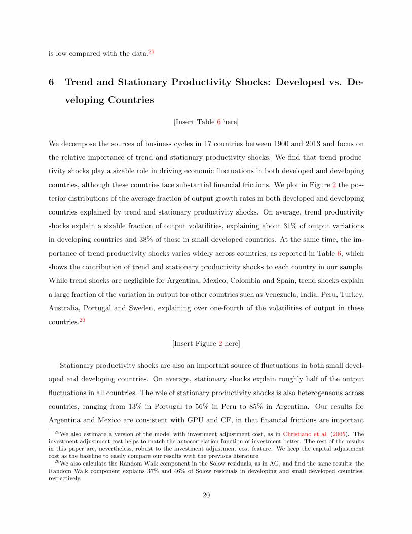
We decompose the sources of business cycles in 17 countries between 1900 and 2013 and focus on

the relative importance of trend and stationary productivity shocks. We find that trend produc-

tivity shocks play a sizable role in driving economic fluctuations in both developed and developing

countries, although these countries face substantial financial frictions. We plot in Figure 2 the pos-

terior distributions of the average fraction of output growth rates in both developed and developing

countries explained by trend and stationary productivity shocks. On average, trend productivity

shocks explain a sizable fraction of output volatilities, explaining about 31% of output variations

in developing countries and 38% of those in small developed countries. At the same time, the im-

portance of trend productivity shocks varies widely across countries, as reported in Table 6, which

shows the contribution of trend and stationary productivity shocks to each country in our sample.

While trend shocks are negligible for Argentina, Mexico, Colombia and Spain, trend shocks explain

a large fraction of the variation in output for other countries such as Venezuela, India, Peru, Turkey,

Australia, Portugal and Sweden, explaining over one-fourth of the volatilities of output in these

countries.26

[Insert Figure 2 here]

Stationary productivity shocks are also an important source of fluctuations in both small devel-

oped and developing countries. On average, stationary shocks explain roughly half of the output

fluctuations in all countries. The role of stationary productivity shocks is also heterogeneous across

countries, ranging from 13% in Portugal to 56% in Peru to 85% in Argentina. Our results for

Argentina and Mexico are consistent with GPU and CF, in that financial frictions are important

25We also estimate a version of the model with investment adjustment cost, as in Christiano et al. (2005). Theinvestment adjustment cost helps to match the autocorrelation function of investment better. The rest of the resultsin this paper are, nevertheless, robust to the investment adjustment cost feature. We keep the capital adjustmentcost as the baseline to easily compare our results with the previous literature.

26We also calculate the Random Walk component in the Solow residuals, as in AG, and find the same results: theRandom Walk component explains 37% and 46% of Solow residuals in developing and small developed countries,respectively.

20

and that trend productivity shocks explain a negligible fraction of output fluctuations for these

two countries. However, unlike in GPU and CF, in our work, the fact that countries face finan-

cial frictions does not preclude trend productivity shocks from having substantial effects on both

developed and developing countries. Additionally, there is no evidence that the cycle is the trend

for emerging economies, and that stationary productivity shocks, which are temporary changes in

productivity, have a limited role in driving business cycles, either. Overall, our estimation paints a

rather different picture about business cycles in small open economies compared with the previous

studies, suggesting that it is important to study several countries.

The reason for the difference between our paper and previous papers is that our estimate utilizes

a much larger data set spanning from 1900 to 2013. AG use a plain-vanilla RBC model and find

that trend productivity shocks are dominant in explaining output fluctuations of Mexico compared

with a much smaller role of trend shocks in Canada. In GPU, the authors argue that long time

series are essential for identifying trend productivity shocks. These authors then point out with

their Argentine data that an RBC model with a dominant trend productivity shock like in AG

cannot satisfy the trade balance behavior of small open economies. Similar to GPU, we use long

time series as they are better suited for identifying trend productivity shocks. Furthermore, as

information from a large set of countries is beneficial for efficiency gain, we collect a rich data set

in order to provide much richer evidence on the sources of business cycles compared with both

studies. In fact, in our data set, consistent with GPU, we find that trend productivity shocks are

not large in Argentina, explaining less than 10% of output fluctuations. However, Argentina turns

out to be a special case. Trend shocks explain over 13% and up to 78% in 12 out of 17 countries

in our sample. Furthermore, the estimated model with financial frictions with a significant role of

trend productivity shocks can match trade balance autocorrelations well, as discussed in Section 5.

Compared with AG, we find that in both Mexico and Canada, financial frictions are significantly

larger than zero, and while trend productivity shocks explain less than 10% of output fluctuations

in Mexico, trend productivity shocks explain around 56% of output fluctuations in Canada. In

other words, AG’s hypothesis that the role of trend shocks distinguishes developing from developed

countries is not supported by richer information from our data set.27

To illustrate the efficiency gain from estimating the model jointly for 17 countries with com-

mon shocks, in Figure 2, we also plot the posterior distributions of the contribution of trend and

27Our result for Mexico is consistent with CF’s result although they use quarterly data after 1980. However, thisresult does not dismiss the use of long-term historical data for many countries in the estimation as we discussedearlier.

21

stationary productivity shocks if we estimate each country individually without common shocks.

When we estimate the model without common shocks, which is the same as estimating each country

individually, we obtain a result similar to our baseline. However, notice that the precision of the

estimates improves in our baseline compared with the individual estimates. In other words, pooling

information from several countries is helpful in more precisely estimating the role of trend produc-

tivity shocks. Furthermore, as discussed later in Section 8, joint estimation for 17 countries helps

us identify an important source of fluctuations in these small open economies: common shocks,

which explain the substantial business cycle comovements across countries.

7 What are Trend and Stationary Productivity Shocks? Devel-

oped vs. Developing Countries


An important contribution of our paper is that by pooling the data, we can also decompose the

importance of trend shocks into the common and country-specific components. Figure 3, which

plots the extracted historical states of world common trend and stationary productivity using the

Kalman smoother at the posterior mean, shows that the estimated common shocks contain actual

world shocks. The common states capture important historical worldwide events, such as the Great

Depression, the two World Wars, the two oil price shocks and the recent Great Recession. These

events appear as large, persistent common productivity shocks to all economies, causing output to

fall in tandem. World War II is associated with a large negative drop in world trend productivity

and a modest drop in world stationary productivity, which recovers quickly at the end of the war.

Another component in the estimated common shocks is the innovation common to all countries

coming from large countries such as the United States. As plotted in Figure 3, the extracted states

move in a direction similar to U.S. output growth rate, which reflects shocks to the U.S. economy

over time. The 2008-2009 Great Recession, starting from the U.S., is captured as a temporary but

sharp drop in productivity.

[Insert Figure 4 around here]

Our analysis of the components of trend productivity shocks finds that although trend pro-

ductivity shocks are about as important in small developed countries as they are in developing

countries, a large component of trend productivity shocks in developed countries is common, while

22

it is country-specific for developing countries. Table 6 shows the fraction of output fluctuations

explained by common trend in each of the 17 countries. On average, the importance of common

trend is about one-third of the total contribution of trend productivity shocks in small developed

countries. In contrast, common trend contributes only 5% of output fluctuations in developing

countries, which is about one-sixth of the fraction of output explained by all trend productivity

shocks. We use the Kalman smoother to calculate the historical output growth rates in each coun-

try, at the posterior mean of the parameters, conditional on common trend and stationary shocks.

We then construct the historical decomposition of output growth rates for developed and develop-

ing countries on average, then plot in Figure 4 a 10-year centered moving average of this historical

decomposition. Over the entire 100 years, common trend productivity shocks play a smaller role

in developing countries than in developed countries. In large events such as the Great Depression

and World War II, which are interpreted as both common trend and stationary productivity shocks

given the persistent movements of macroeconomic variables, developing countries are more affected

by common stationary productivity shocks, while for developed countries, it is a common trend.

For example, between 1940 and 1949, about 25% of output fluctuations in small developed countries

is explained by common trend shocks, while it is only 15% in developing countries.

We interpret these results as follows. Small developed countries are, in general, closer to the

frontier of world technology, so they are more affected by common trend. On the other hand,

developing countries are marked by frequent regime switches and policy changes domestically, so

the trend that is important for them is country-specific. These results suggest that while trend

productivity shocks are an important source of business cycles in both developed and developing

countries, these trend shocks capture different phenomena in these two groups of countries.

8 Common Shocks

This section addresses the question regarding the extent to which business cycles in small open

economies are driven by outside shocks. We aggregate all types of common shocks and show that

they play an important role in both groups of small open economies in the last 100 years. We

also briefly discuss our results compared with the results obtained by the reduced-form estimation

approach frequently used in the previous literature on common shocks.


23

First, the model with common shocks matches the cross-country correlation in our data rela-

tively well, as reported in the last row of Table 5, which shows the average cross-country output

and consumption correlations implied by the model.28 Without common shocks, the model would

imply no correlation in output and other aggregate variables.


Second, while the effects of common shocks are heterogeneous across countries, world common

shocks contribute to a substantially large fraction of fluctuations in these countries. On average,

28% of the fluctuations in output, 22% in consumption, 22% in investment, and 22% in trade

balance between 1900 and 2013 can be attributed to all types of common shocks, as reported in

the last row of Table 7. Common shocks are of similar importance for both small developed and

developing countries. This result reflects the substantial comovements of these countries in history,

especially during major historical episodes, such as the Great Depression, which are captured in the

extracted world common shocks. Figure 5 plots the output growth rates of Argentina and Canada

along with the output growth rates conditional on common shocks only and on country-specific

shocks only. The estimated common shocks explain a large fraction of the output fluctuations in

both countries, especially during worldwide events such as the Great Depression, World War I and

II, the two oil price shocks and the recent Great Recession. We note that the estimated country-

specific shocks are reasonable, which is demonstrated by the 2001 crisis in Argentina: during this

period, Argentina’s decline in output is mostly explained by country-specific shocks, as expected.

A historical decomposition exercise shows that the role of common shocks varies over time for

both developed and developing countries. In particular, common shocks explain a large fraction of

output variations in all countries in the first half of the 20th century during historical episodes as in

Figure 4, which plots a 10-year centered moving average of the historical decomposition of output

fluctuations for small developed and developing countries, using the Kalman smoother. During

the Great Depression and World War II, common shocks play a similar role for both groups of

countries, explaining up to 50% of output fluctuations. This result reflects the worldwide impact of

these disasters on all countries. In the later periods of the 20th century, these small open economies

went through fewer large turbulences caused by common shocks, limiting the role of these common

shocks, especially in developing countries. For example, during the 1950–70 period, common shocks

explain around 20% of output fluctuations. Starting in the early 1970s, there were two oil price

28We also show that there is a positive relationship between correlations and contribution of common shocks inAppendix Figure A4, as common shocks have to explain both static and dynamic correlations across countries.

24

shocks, and small developed countries were severely hit by these common shocks, so a larger fraction

of output volatility (up to 40% in small developed countries) is explained by common shocks. At

the same time, these shocks have smaller impacts on developing countries—about 30%. Recently,

the importance of common shocks increases, but declines again after the 2008-2009 recession. Our

result of recent periods is consistent with the report in the October 2013 World Economic Outlook,

which documents that output synchronized more in the Great Recession but that synchronization

has declined again recently.

Third, a structural analysis allows us to identify several types of common shocks important

for business cycles in small open economies. In particular, we find that not only trend and sta-

tionary productivity common shocks, but also country premium and preference common shocks

play a non-negligible role in business cycle fluctuations in small open economies. Among all com-

mon shocks, productivity shocks are the most important for output, as displayed in Table 7. On

average, common stationary productivity shocks explain 18% of output fluctuations and common

trend productivity shocks contribute another 8%. Consumption volatilities are explained by both

common productivity shocks and common preference shocks, accounting for about 17% and 3% of

consumption volatility, respectively. The reason for this result is as follows. When debt adjustment

cost φjD is high, preference shocks help to generate the excess volatility of consumption relative to

output. As consumption is correlated across countries, the estimation assigns a non-negligible role

to common preference shocks.

Common interest rate premium and spending shocks do not explain much of the movements in

output and consumption, but account for a sizable fraction of the fluctuations in investment and

the trade balance. For example, common interest rate premium shocks account for over 14% of the

trade balance variations and 8% of investment. The reason for this result is that when households

are not able to lend and borrow internationally easily, interest rate premium shocks help to explain

more of the behavior of the trade balance. Since the trade balance is correlated across countries, the

role of common interest rate premium shocks is non-negligible. Additionally, the fact that different

types of shocks explain the comovements of different aggregate variables is consistent with other

papers in the small open economy literature, such as Adolfson et al. (2007) and others.

In one of the extensions, we estimate the baseline model in which each shock has not only world

common but also group-specific shocks in addition to their country-specific shocks. For example,

25

the stationary productivity shock process is given by:

ajt = (act)vacj (agt )

vagjajt , (23)

where vagj governs the effect of the group-specific shock on each country, and agt follows an AR(1)

process, i.e., log agt = ρag log agt−1+εag ,t, εag ,t ∼ N(0, 1). The small developed and developing group-

specific shocks capture the common shocks specific to these two groups of countries. We find that

both world common and group-specific shocks explain roughly 48% of the output fluctuations, 40%

of consumption fluctuations and 30% of trade balance in small open economies. In addition, our

baseline results, such as the roles of financial frictions and trend productivity shocks in small open

economies, are robust.


Finally, we compare the importance of common shocks in our DSGE estimation with that

in the reduced-form DFM. We first note that although a reduced-form DFM approach can also

estimate the importance of common shocks, our structural approach is much more suitable for

the focus of our analysis. In particular, using the DSGE estimation allows us to characterize the

important features of business cycles in small open economies, such as financial frictions and the

nature of trend productivity shocks, while the DFM approach does not provide either transmission

mechanisms or structural interpretation of the estimates. Another difference between our approach

and the DFM is that while our model can identify several types of common shocks, the typical

DFM approach in Kose et al. (2003) and Kose et al. (2012) has one type of common shock, which

matters for the total contribution of common shocks.29 To illustrate the difference, we estimate the

role of common shocks using the DFM approach. As reported in Table 8, the mean contribution

of world common shocks is roughly 11% of output fluctuation—less than half of the structural

estimation. The discrepancies are also large for other variables. The difference between the DSGE

estimation and the DFM estimation may come from the assumption of one common factor in the

DFM approach. To check this explanation, we run the same exercise for the data generated from

our baseline model evaluated at the posterior mean of the parameters. Again, we find that the DFM

29The standard model isyit = ai + bworldi fworldt + bcountryi fcountryt + εit, (24)

where yit is a vector of aggregate variables for country i at time t, fworldt is the world common factor with a loadingbworldi that varies across countries, fcountryt is the country factor with a corresponding loading bcountryi . The commonfactor, fworldt , country factor fcountryt and the idiosyncratic component εit, are assumed to follow AR(p) processes.

26

estimation does not fully capture the extent of common shocks in the data-generating process. In

particular, the DFM estimation attributes less than 12% of output fluctuations to common shocks

in all of the generated data, while in the data-generating process, common shocks explain nearly

30% of output fluctuations.30 It is possible that a DFM estimation with multiple common shocks

may be able to reconcile with our results.31 However, as discussed earlier, the DFM approach is

not suitable for our focus.

9 Subsample Stability

This section characterizes business cycles in small open economies, focusing on the difference be-

tween the first and the second half of the sample.


Throughout the paper, we motivate the use of historical data by the fact that long data series

contain several business cycles, which helps to better identify trend shocks. Nevertheless, a valid

concern is that business cycles in many small open economies may have changed over time. For

example, aggregate volatilities have decreased after World War II, as shown for small developed

countries in Table 2a. To address this concern, we estimate the baseline model with two subsamples:

1901–1950 and 1951–2013. The basis for dividing the data in 1950 is that second moment statistics

suggest that the volatility in business cycles have decreased after 1950, especially in small developed

countries. We do not estimate the 1980–2013 period because the short span data have limited

number of observations, and the second moment statistics for this period are not substantially

different from those in the 1951–2013 period. In the interest of space, we summarize the results in

Table 9.

First, we find that financial frictions are an important feature in business cycles for both small

developed and developing countries over both subsamples. In both periods, the two parameters

governing the elasticity of the real interest rate to the debt-to-output level and expected productivity

are substantially different from zero and vary strongly across countries. As plotted in Figure 6, the

30We simulate the baseline model using the posterior means of the parameters and generate 240 samples of thesame length and dimension as the actual data. The median of the share of variances of output explained by commonshocks is 10.5% with a 5-95% confidence interval of (1.43%, 22.6%). The medians for consumption, investment andthe trade balance are 5.59%, 4.18% and 10.1%, respectively. Detailed results are available upon request.

31One support for the existence of multiple factors in our data is that the principle component analysis shows thatthe first component explains about 15% of the variances, while each of the next four components explain between 5%and 9% of the data.

27

debt-elastic parameter φjD for many developing economies, as well as Spain, is higher in the first

half of the 20th century than in the second half of the sample. The elasticity of the real interest

rate to expected productivity φjSR is slightly larger in the second half of the sample in most of the

countries in our sample. In other words, the extent to which countries face financial frictions has

changed over time.


Second, trend shocks on average explain about one-third of output fluctuations, and stationary

productivity shocks contribute to about one-half of output fluctuations in both sample periods for

both groups of countries, as reported in Table 9. In both subsamples, the third and fourth panels

of Figure 6 show that the volatilities in both Argentina and Mexico are attributed mostly to the

stationary productivity shocks, consistent with CF results for Mexican data between 1980Q1 and

2003Q2. However, the role of trend shocks is substantial for other small open economies. For

example, trend shocks explain around 40% of the variations in output in the 1951–2013 period for

Brazil, Chile, India, Taiwan, and Norway.

Lastly, common shocks are more important in the 1901-1950 period than in the 1951–2013

period in developing countries, while the difference in the contribution of common shocks to output

between two subperiods for developed countries is less pronounced. This result is consistent with

the historical variance decomposition exercise in our baseline estimation.

Overall, the results obtained in the subsample analysis suggest that although the volatilities

of business cycles in small open economies have become smaller over time, and although we also

find changes in the estimated parameters in the model, the main messages of our paper are robust.

In particular, we find that trend productivity shocks and common shocks play a sizable role in

business cycles in these countries. Additionally, financial frictions are still an important feature for

small open economies, although the degree of financial frictions changes over time.32

32We also estimate a few variations of the baseline model. For example, since productivity shocks in the UnitedStates can also affect the world interest rate, we assume that there is a correlation between the two common produc-tivity shocks and common premium shocks. Another variation of the baseline model is the country interest rate shockspecification that separates the effects of expected trend productivity shocks and expected stationary productivityshocks. We consider a case where the normalized Solow residuals are normalized by Xt−1 instead of Xt as in thebaseline. The estimation results are all similar to the baseline results.

28

10 Conclusion

In this paper, we characterize business cycles in small open economies over the long horizon.

We find strong evidence that an RBC model with reduced-form financial frictions and common

shocks provides a good description of business cycles in both developing and developed small

open economies. Estimating the model with a new data set covering 17 countries, we find that

the reduced-form financial frictions in our model are substantial in many countries. This finding

resonates with recent work by Akinci (2014) and Fernandez and Gulan (2015) who quantify the

role of financial frictions in a micro-founded financial friction model and match moments calculated

using data for emerging economies. Furthermore, unlike the two extreme findings in AG and GPU,

we document a sizable but not dominant role for trend productivity shocks. Our estimates also

find that common trend productivity shocks are much more important than country-specific trend

shocks in small developed countries while the reverse is true in developing countries. We interpret

this as reflecting the fact that developing countries face frequent changes in domestic policies and

regimes, making country-specific trend shocks more important than common trend shocks.

Our analysis points out the large role of common shocks in small open economies. In particular,

common trend and stationary productivity shocks explain the bulk of output fluctuations in both

developing and developed small open economies. These common productivity shocks may capture

not only true technology shocks, but also permanent and transitory changes in the terms of trade

in these small open economies. These results suggest that future research should investigate the

transmission mechanism of shocks and the general equilibrium effects from large countries to small

open countries through international trade of both goods and financial assets. Furthermore, since

this paper assumes that all common shocks are exogenous and outside of these 17 countries, future

research can explicitly model the trade and financial linkages between these countries to take into

account the effects of idiosyncratic shocks from the estimated common shocks. Further analysis

in those models with endogenous transmission of shocks across countries may be able to shed

more light on the role of external policies in mitigating the effects of outside shocks on small open

economies.

29

References

Adolfson, M., S. Laseen, J. Linde and M. Villani, “Bayesian estimation of an open economy

DSGE model with incomplete pass-through,” Journal of International Economics 72 (July 2007),

481–511.

Aguiar, M. and G. Gopinath, “Emerging Market Business Cycles: The cycle is the trend,”

Journal of Political Economy 115 (2007), 69–102.

Akinci, O., “Financial Frictions and Macroeconomic Fluctuations in Emerging Economies,” In-

ternational Finance Discussion Papers 1120, 2014.

Alvarez-Parra, F., L. Brandao-Marques and M. Toledo, “Durable goods, financial fric-

tions, and business cycles in emerging economies,” Journal of Monetary Economics 60 (2013),

720–736.

Arellano, C., “Default Risk and Income Fluctuations in Emerging Economies,” American Eco-

nomic Review 98 (2008), 690–712.

Barro, R. and J. Ursua, “Macroeconomic Data,” Technical Report, 2010, data set.

Chang, R. and A. Fernandez, “On the Sources of Aggregate Fluctuations in Emerging

Economies,” International Economic Review 54 (Nov 2013), 1267–1295.

Christiano, L. J., M. Eichenbaum and C. L. Evans, “Nominal Rigidities and the dynamic

effects of a shock to Monetary Policy,” Journal of Political Economy 113 (February 2005), 1–45.

Crucini, M. and K. Chen, “General and Partial Equilibrium Approaches to the Study of Real

Business Cycles,” Working Paper, November 2011.

Fernandez, A., A. Gonzalez and D. Rodriguez, “Sharing a Ride in the Commodities Roller

Coaster: Common Factors in Business Cycles of Emerging Economies,” Working Paper, 2015.

Fernandez, A. and A. Gulan, “Interest rates, Leverage and Business Cycles in Emerging

Economies: The role of financial frictions,” American Economic Journal: Macroeconomics 7

(2015), 153–188.

Fernandez-Villaverde, J., P. Guerron-Quintana, J. F. Rubio-Ramırez and M. Uribe,

“Risk Matters: The real effects of volatility shocks,” American Economic Review 101 (2011),

2530–2561.

30

Garcia-Cicco, J., R. Pancrazi and M. Uribe, “Real Business Cycles in Emerging Countries?,”

American Economic Review 100 (Dec 2010), 2510–2531.

Glick, R. and K. Rogoff, “Global versus country-specific productivity shocks and the current

account,” Journal of Monetary Economics 35 (1995), 159–192.

Gregory, A. and A. Head, “Common and country-specific fluctuations in productivity, invest-

ment, and the current account,” Journal of Monetary Economics 44 (1999), 423–451.

Guerron-Quintana, P., “Common and idiosyncratic disturbances in developed small open

economies,” Journal of International Economics 90 (2013), 33–49.

Haario, H., E. Saksman and J. Tamminen, “An adaptive Metropolis algorithm,” Bernoulli 7

(2001), 223–242.

Kose, M., “Explaining business cycles in small open economies: How much do world prices mat-

ter?,” Journal of International Economics 56 (2002), 299–327.

Kose, M., C. Otrok and E. Prasad, “Global business cycles: convergence or decoupling?,”

International Economic Review (2012).

Kose, M., C. Otrok and C. Whiteman, “International business cycles: World, region, and

country-specific factors,” American Economic Review 93 (2003), 1216–1239.

Mendoza, E. G., “Real business cycles in a small open economy,” American Economic Review

81 (September 1991), 797–818.

Nakamura, E., D. Sergeyev and J. Steinsson, “Growth-Rate and Uncertainty Shocks in

Consumption: Cross-Country Evidence,” Working paper, 2014.

Naoussi, C. F. and F. Tripier, “Trend shocks and economic development,” Journal of Devel-

opment Economics 103 (2013), 29–42.

Neumeyer, P. and F. Perri, “Business cycles in emerging economies: the role of interest rates,”

Journal of Monetary Economics 52 (March 2005), 345–380.

Romer, C., “Changes in Business Cycles: Evidence and Explanations,” Journal of Economic

Perspectives 13 (1999), 23–44.

31

Rondeau, S., “Sources of Fluctuations in Emerging Markets : DSGE Estimation with Mixed

Frequency Data,” (2012), 1–31.

Schmitt-Grohe, S. and M. Uribe, “Solving Dynamic General Equilibrium Models Using a

Second-Order Approximation to the Policy Function,” Journal of Economic Dynamics and Con-

trol 28 (2004), 755–775.

Uribe, M. and V. Z. Yue, “Country spreads and emerging countries: Who drives whom?,”

Journal of International Economics 69 (2006), 6–36.

32

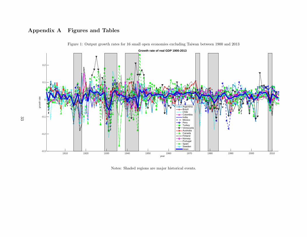
Appendix A Figures and Tables

Figure 1: Output growth rates for 16 small open economies excluding Taiwan between 1900 and 2013

year1910 1920 1930 1940 1950 1960 1970 1980 1990 2000 2010

grow

th r

ate

-0.3

-0.2

-0.1

0

0.1

0.2

Growth rate of real GDP 1900-2013

ArgentinaBrazilChileColombiaIndiaMexicoPeruTurkeyVenezuelaAustraliaCanadaFinlandNorwayPortugalSpainSwedenmean

Notes: Shaded regions are major historical events.

33

Figure 2: Trend vs stationary productivity shocks

0 0.2 0.4 0.6 0.8 1

dens

ity

0

2

4

6

8

10

12EM Trend

0 0.2 0.4 0.6 0.8 1

dens

ity

0

2

4

6

8

10

12DEV Trend

0 0.2 0.4 0.6 0.8 1

dens

ity

0

2

4

6

8

10

12EM Stationary

0 0.2 0.4 0.6 0.8 1

dens

ity

0

2

4

6

8

10

12DEV Stationary

baselineindividual

Note: “EM trend”, “EM stationary” are the posterior distributions of the fraction of output indeveloping countries, on average, explained by trend and stationary productivity shocks, respec-tively. “DEV trend”, “DEV stationary” are the posterior distributions of the fraction of outputin small developed countries, on average, explained by trend and stationary productivity shocks,respectively. In each graph, we compare the posterior distribution estimated in our baseline model(baseline) with that estimated in the model without common shocks (individual).

34

Figure 3: Recovered world common states (solid line) against U.S. annual output growth rate (dashed line)between 1900 and 2013.

1910 1920 1930 1940 1950 1960 1970 1980 1990 2000 2010

stat

e

-6

-4

-2

0

2

World common 7

U.S

. GD

P

-0.1

-0.05

0

0.05

0.1

0.15

1910 1920 1930 1940 1950 1960 1970 1980 1990 2000 2010

stat

e 0

World common a

U.S

. GD

P

0

StateU.S. GDP

Notes: µ is the trend productivity shocks and a is the stationary productivity shocks. Therecovered states were calculated using Kalman smoother at the posterior mean of the estimatedparameters. Shaded regions are major historical events.

Figure 4: The contribution of common shocks to output on average in developing and small developedcountries weighted over 10-year centered moving average window between 1905 and 2008.

year1920 1940 1960 1980 2000

perc

enta

ge

0

10

20

30

40

50

60EM historical variance decomposition

All common shocks contributionCommon stationaryCommon trend

year1920 1940 1960 1980 2000

perc

enta

ge

0

10

20

30

40

50DEV historical variance decomposition

Note: This figure is constructed from the historical decomposition of output: the fraction ofoutput in each point in time explained by common shocks. EM denotes average for emergingeconomies while DEV denotes average for small developed countries.

35

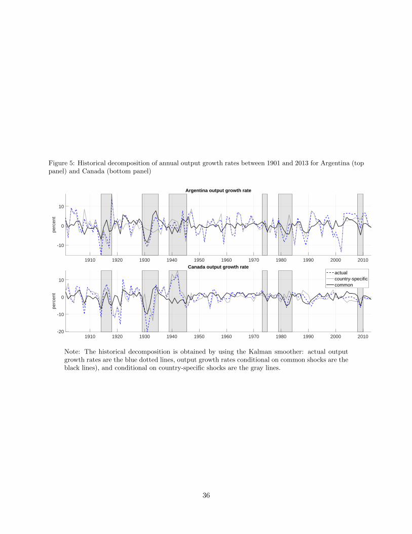
Figure 5: Historical decomposition of annual output growth rates between 1901 and 2013 for Argentina (toppanel) and Canada (bottom panel)

1910 1920 1930 1940 1950 1960 1970 1980 1990 2000 2010

perc

ent

-10

0

10

Argentina output growth rate

1910 1920 1930 1940 1950 1960 1970 1980 1990 2000 2010

perc

ent

-20

-10

0

10

Canada output growth rateactualcountry-specificcommon

Note: The historical decomposition is obtained by using the Kalman smoother: actual outputgrowth rates are the blue dotted lines, output growth rates conditional on common shocks are theblack lines), and conditional on country-specific shocks are the gray lines.

36

Figure 6: Subsample stability

Argentina Brazil Chile Colombia India Mexico Peru Taiwan Turkey Ven Aus Canada Finland Norway Portugal Spain Sweden0

1

2

3

4

5?D

1900--20131901--19501951--2013


1

2

3?SR


0.2

0.4

0.6

0.8Contribution of Trend shocks


0.2

0.4

0.6

0.8

1Contribution of Stationary shocks


0.2

0.4

0.6

0.8

1Contribution of Common shocks

Notes: The numbers are calculated at the mean of the posterior distributions for eachcountry in three periods: 1900–2013, 1901–1950 and 1951–2013. The contribution oftrend, stationary productivity shocks and common shocks are calculated as the fractionof output fluctuations in each country explained by these shocks.37

Table 1: Second moments: 1900–2013

Standard deviations Correlation with output Correlation with TBY Autocorrelation

Y C I TBY C I TBY C I Y C I TBY

(1) (2) (3) (4) (5) (6) (7) (8) (9) (10) (11) (12) (13)

Developing

Argentina 5.36 7.41 19.84 5.06 0.74 0.66 -0.02 -0.25 -0.19 0.13 0.01 0.31 0.59Brazil 4.04 7.30 20.98 3.47 0.49 0.41 -0.17 -0.15 0.02 0.19 -0.26 0.17 0.71Chile 6.12 9.13 23.51 7.79 0.64 0.55 0.18 -0.02 -0.07 0.10 0.08 0.05 0.79Colombia 2.36 5.92 17.31 3.57 0.55 0.27 -0.13 -0.08 -0.22 0.30 -0.23 -0.21 0.75India 3.45 4.28 11.74 1.95 0.59 0.23 -0.39 -0.31 -0.12 0.23 -0.07 0.09 0.87Mexico 4.19 6.01 19.28 4.14 0.67 0.56 -0.17 -0.28 -0.06 0.00 -0.09 0.22 0.73Peru 4.86 4.83 17.38 4.51 0.83 0.74 0.04 -0.02 -0.01 0.43 0.29 0.30 0.71Taiwan 8.89 8.90 21.53 5.62 0.84 0.23 0.03 -0.06 -0.07 0.34 0.28 -0.04 0.78Turkey 7.15 6.24 14.19 3.53 0.66 0.46 -0.12 -0.19 -0.16 -0.17 0.09 0.17 0.82Venezuela 7.49 10.11 20.06 7.14 0.65 0.83 -0.06 -0.11 -0.21 0.49 -0.05 0.37 0.60

Mean 5.39 7.01 18.58 4.68 0.67 0.49 -0.08 -0.15 -0.11 0.20 0.00 0.14 0.73

Small Developed

Australia 3.16 4.97 13.12 3.71 0.28 0.42 0.04 -0.09 -0.16 0.50 0.15 0.34 0.45Canada 5.03 4.49 12.74 3.86 0.70 0.50 0.13 0.16 -0.01 0.36 0.03 0.45 0.81Finland 4.73 5.97 14.12 5.75 0.79 0.51 0.20 0.13 0.14 0.26 0.14 0.18 0.79Norway 3.79 4.72 14.72 8.67 0.82 0.68 -0.08 -0.05 -0.14 0.00 -0.06 -0.15 0.94Portugal 4.61 4.44 13.37 5.04 0.83 0.35 0.02 -0.12 -0.18 -0.02 0.20 0.17 0.79Spain 4.50 8.08 11.98 2.42 0.85 0.49 -0.15 -0.19 -0.07 0.30 -0.05 0.39 0.74Sweden 3.51 4.30 10.32 3.34 0.67 0.69 -0.09 -0.21 -0.05 -0.02 -0.09 0.17 0.80

Mean 4.19 5.28 12.91 4.68 0.71 0.52 0.01 -0.05 -0.07 0.20 0.05 0.22 0.76

38

Table 2: Average second moments in developed and developing countries

(a) Second moments across countries: Different periods

Standard deviations Correlation with output Correlation with TBY Autocorrelation

Y C I TBY C I TBY C I Y C I TBY

All1900–2013 4.90 6.30 16.25 4.68 0.68 0.50 -0.04 -0.11 -0.09 0.20 0.02 0.18 0.751900–1950 6.24 8.43 21.42 4.43 0.65 0.43 -0.04 -0.15 -0.13 0.10 -0.06 0.18 0.631951–2013 3.44 4.06 10.90 3.87 0.73 0.65 -0.08 -0.13 -0.12 0.30 0.21 0.19 0.69

EM1900–2013 5.39 7.01 18.58 4.68 0.67 0.49 -0.08 -0.15 -0.11 0.20 0.00 0.14 0.731900–1950 6.73 9.27 24.58 4.35 0.60 0.40 -0.10 -0.20 -0.16 0.09 -0.10 0.17 0.601951–2013 4.03 4.93 12.56 4.06 0.75 0.69 -0.10 -0.16 -0.15 0.25 0.18 0.13 0.72

DEV1900–2013 4.19 5.28 12.91 4.68 0.71 0.52 0.01 -0.05 -0.07 0.20 0.05 0.22 0.761900–1950 5.56 7.24 16.91 4.55 0.71 0.48 0.04 -0.07 -0.09 0.10 -0.01 0.19 0.681951–2013 2.60 2.82 8.52 3.60 0.71 0.60 -0.04 -0.09 -0.08 0.37 0.25 0.28 0.65

(b) Average cross-country correlations: Different periods

Y C I TBY

ALL EM DEV ALL EM DEV ALL EM DEV ALL EM DEV

1900–2013 0.14 0.15 0.23 0.07 0.06 0.15 0.18 0.20 0.19 0.09 0.21 0.041900–1950 0.15 0.19 0.19 0.09 0.09 0.15 0.22 0.26 0.18 0.17 0.28 0.011951–2013 0.14 0.13 0.34 0.03 0.02 0.17 0.12 0.12 0.23 0.07 0.09 0.16

Notes: The numbers are calculated as averages across all 17 countries (All), 10 developing coun-tries (Developing) and seven small developed countries (Developed) in three periods: 1900–2013,1950–2013 and 1980–2013. Y denotes the growth rate of output, C denotes the growth rate ofconsumption, I denotes the growth rate of investment, and TBY denotes trade balance-to-outputratio.

39

Table 3: Calibrated parameters

Parameter Description Value

σ Risk aversion 2α Capital share 0.32θ Labor elasticity 1.6β Discount rate 0.9224

Table 4: Baseline posterior estimates

(a) Common shocks parameters

ρµc B 0.62(0.5, 0.2) (0.52, 0.72)

ρac B 0.73(0.5, 0.2) (0.67, 0.79)

ρpmc B 0.88(0.5, 0.2) (0.81, 0.95)

ρbc B 0.91(0.5, 0.2) (0.88, 0.94)

ρgc B 0.76(0.5, 0.2) (0.68, 0.83)

Notes: All results in Tables 4a, 4b, and 4c are reported using eight chains of 1 mil-lion draws each with half burn-in from the posterior distribution. The numbers inparentheses for the posterior are the 5% and 95% confidence interval of the poste-rior distribution. B denotes Beta distribution, G denotes Gamma distribution and Udenotes Uniform distribution.

40

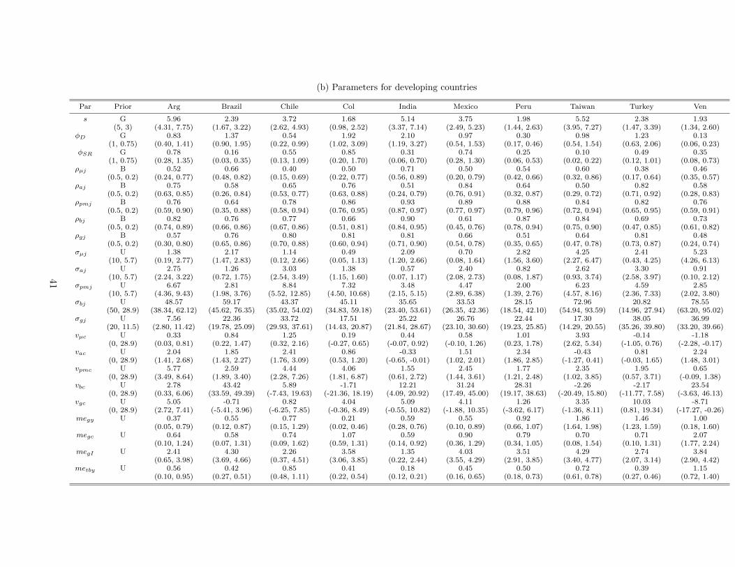
(b) Parameters for developing countries

Par Prior Arg Brazil Chile Col India Mexico Peru Taiwan Turkey Ven

s G 5.96 2.39 3.72 1.68 5.14 3.75 1.98 5.52 2.38 1.93(5, 3) (4.31, 7.75) (1.67, 3.22) (2.62, 4.93) (0.98, 2.52) (3.37, 7.14) (2.49, 5.23) (1.44, 2.63) (3.95, 7.27) (1.47, 3.39) (1.34, 2.60)

φD G 0.83 1.37 0.54 1.92 2.10 0.97 0.30 0.98 1.23 0.13(1, 0.75) (0.40, 1.41) (0.90, 1.95) (0.22, 0.99) (1.02, 3.09) (1.19, 3.27) (0.54, 1.53) (0.17, 0.46) (0.54, 1.54) (0.63, 2.06) (0.06, 0.23)

φSR G 0.78 0.16 0.55 0.85 0.31 0.74 0.25 0.10 0.49 0.35(1, 0.75) (0.28, 1.35) (0.03, 0.35) (0.13, 1.09) (0.20, 1.70) (0.06, 0.70) (0.28, 1.30) (0.06, 0.53) (0.02, 0.22) (0.12, 1.01) (0.08, 0.73)

ρµj B 0.52 0.66 0.40 0.50 0.71 0.50 0.54 0.60 0.38 0.46(0.5, 0.2) (0.24, 0.77) (0.48, 0.82) (0.15, 0.69) (0.22, 0.77) (0.56, 0.89) (0.20, 0.79) (0.42, 0.66) (0.32, 0.86) (0.17, 0.64) (0.35, 0.57)

ρaj B 0.75 0.58 0.65 0.76 0.51 0.84 0.64 0.50 0.82 0.58(0.5, 0.2) (0.63, 0.85) (0.26, 0.84) (0.53, 0.77) (0.63, 0.88) (0.24, 0.79) (0.76, 0.91) (0.32, 0.87) (0.29, 0.72) (0.71, 0.92) (0.28, 0.83)

ρpmj B 0.76 0.64 0.78 0.86 0.93 0.89 0.88 0.84 0.82 0.76(0.5, 0.2) (0.59, 0.90) (0.35, 0.88) (0.58, 0.94) (0.76, 0.95) (0.87, 0.97) (0.77, 0.97) (0.79, 0.96) (0.72, 0.94) (0.65, 0.95) (0.59, 0.91)

ρbj B 0.82 0.76 0.77 0.66 0.90 0.61 0.87 0.84 0.69 0.73(0.5, 0.2) (0.74, 0.89) (0.66, 0.86) (0.67, 0.86) (0.51, 0.81) (0.84, 0.95) (0.45, 0.76) (0.78, 0.94) (0.75, 0.90) (0.47, 0.85) (0.61, 0.82)

ρgj B 0.57 0.76 0.80 0.81 0.81 0.66 0.51 0.64 0.81 0.48(0.5, 0.2) (0.30, 0.80) (0.65, 0.86) (0.70, 0.88) (0.60, 0.94) (0.71, 0.90) (0.54, 0.78) (0.35, 0.65) (0.47, 0.78) (0.73, 0.87) (0.24, 0.74)

σµj U 1.38 2.17 1.14 0.49 2.09 0.70 2.82 4.25 2.41 5.23(10, 5.7) (0.19, 2.77) (1.47, 2.83) (0.12, 2.66) (0.05, 1.13) (1.20, 2.66) (0.08, 1.64) (1.56, 3.60) (2.27, 6.47) (0.43, 4.25) (4.26, 6.13)

σaj U 2.75 1.26 3.03 1.38 0.57 2.40 0.82 2.62 3.30 0.91(10, 5.7) (2.24, 3.22) (0.72, 1.75) (2.54, 3.49) (1.15, 1.60) (0.07, 1.17) (2.08, 2.73) (0.08, 1.87) (0.93, 3.74) (2.58, 3.97) (0.10, 2.12)

σpmj U 6.67 2.81 8.84 7.32 3.48 4.47 2.00 6.23 4.59 2.85(10, 5.7) (4.36, 9.43) (1.98, 3.76) (5.52, 12.85) (4.50, 10.68) (2.15, 5.15) (2.89, 6.38) (1.39, 2.76) (4.57, 8.16) (2.36, 7.33) (2.02, 3.80)

σbj U 48.57 59.17 43.37 45.11 35.65 33.53 28.15 72.96 20.82 78.55(50, 28.9) (38.34, 62.12) (45.62, 76.35) (35.02, 54.02) (34.83, 59.18) (23.40, 53.61) (26.35, 42.36) (18.54, 42.10) (54.94, 93.59) (14.96, 27.94) (63.20, 95.02)

σgj U 7.56 22.36 33.72 17.51 25.22 26.76 22.44 17.30 38.05 36.99(20, 11.5) (2.80, 11.42) (19.78, 25.09) (29.93, 37.61) (14.43, 20.87) (21.84, 28.67) (23.10, 30.60) (19.23, 25.85) (14.29, 20.55) (35.26, 39.80) (33.20, 39.66)

vµc U 0.33 0.84 1.25 0.19 0.44 0.58 1.01 3.93 -0.14 -1.18(0, 28.9) (0.03, 0.81) (0.22, 1.47) (0.32, 2.16) (-0.27, 0.65) (-0.07, 0.92) (-0.10, 1.26) (0.23, 1.78) (2.62, 5.34) (-1.05, 0.76) (-2.28, -0.17)

vac U 2.04 1.85 2.41 0.86 -0.33 1.51 2.34 -0.43 0.81 2.24(0, 28.9) (1.41, 2.68) (1.43, 2.27) (1.76, 3.09) (0.53, 1.20) (-0.65, -0.01) (1.02, 2.01) (1.86, 2.85) (-1.27, 0.41) (-0.03, 1.65) (1.48, 3.01)

vpmc U 5.77 2.59 4.44 4.06 1.55 2.45 1.77 2.35 1.95 0.65(0, 28.9) (3.49, 8.64) (1.89, 3.40) (2.28, 7.26) (1.81, 6.87) (0.61, 2.72) (1.44, 3.61) (1.21, 2.48) (1.02, 3.85) (0.57, 3.71) (-0.09, 1.38)

vbc U 2.78 43.42 5.89 -1.71 12.21 31.24 28.31 -2.26 -2.17 23.54(0, 28.9) (0.33, 6.06) (33.59, 49.39) (-7.43, 19.63) (-21.36, 18.19) (4.09, 20.92) (17.49, 45.00) (19.17, 38.63) (-20.49, 15.80) (-11.77, 7.58) (-3.63, 46.13)

vgc U 5.05 -0.71 0.82 4.04 5.09 4.11 1.26 3.35 10.03 -8.71(0, 28.9) (2.72, 7.41) (-5.41, 3.96) (-6.25, 7.85) (-0.36, 8.49) (-0.55, 10.82) (-1.88, 10.35) (-3.62, 6.17) (-1.36, 8.11) (0.81, 19.34) (-17.27, -0.26)

megy U 0.37 0.55 0.77 0.21 0.59 0.55 0.92 1.86 1.46 1.00(0.05, 0.79) (0.12, 0.87) (0.15, 1.29) (0.02, 0.46) (0.28, 0.76) (0.10, 0.89) (0.66, 1.07) (1.64, 1.98) (1.23, 1.59) (0.18, 1.60)

megc U 0.64 0.58 0.74 1.07 0.59 0.90 0.79 0.70 0.71 2.07(0.10, 1.24) (0.07, 1.31) (0.09, 1.62) (0.59, 1.31) (0.14, 0.92) (0.36, 1.29) (0.34, 1.05) (0.08, 1.54) (0.10, 1.31) (1.77, 2.24)

megI U 2.41 4.30 2.26 3.58 1.35 4.03 3.51 4.29 2.74 3.84(0.65, 3.98) (3.69, 4.66) (0.37, 4.51) (3.06, 3.85) (0.22, 2.44) (3.55, 4.29) (2.91, 3.85) (3.40, 4.77) (2.07, 3.14) (2.90, 4.42)

metby U 0.56 0.42 0.85 0.41 0.18 0.45 0.50 0.72 0.39 1.15(0.10, 0.95) (0.27, 0.51) (0.48, 1.11) (0.22, 0.54) (0.12, 0.21) (0.16, 0.65) (0.18, 0.73) (0.61, 0.78) (0.27, 0.46) (0.72, 1.40)

41

(c) Parameters for developed countries

Par Prior Australia Canada Finland Norway Portugal Spain Sweden

s G 4.37 4.57 3.92 1.43 2.71 6.96 5.96(5, 3) (2.96, 5.98) (3.48, 5.84) (2.73, 5.28) (0.96, 1.96) (1.83, 3.70) (4.94, 9.29) (3.84, 8.36)

φD G 2.12 0.67 0.48 0.46 0.11 1.02 0.41(1, 0.75) (1.22, 3.23) (0.42, 0.97) (0.26, 0.78) (0.20, 0.81) (0.07, 0.17) (0.63, 1.52) (0.20, 0.70)

φSR G 0.33 0.17 0.44 1.19 0.27 0.24 0.96(1, 0.75) (0.06, 0.73) (0.03, 0.38) (0.11, 0.88) (0.56, 1.95) (0.05, 0.61) (0.05, 0.50) (0.41, 1.61)

ρµj B 0.62 0.62 0.51 0.55 0.41 0.55 0.48(0.5, 0.2) (0.33, 0.82) (0.52, 0.72) (0.24, 0.77) (0.24, 0.85) (0.27, 0.54) (0.23, 0.82) (0.25, 0.68)

ρaj B 0.65 0.58 0.71 0.66 0.60 0.93 0.77(0.5, 0.2) (0.34, 0.88) (0.29, 0.81) (0.63, 0.79) (0.57, 0.75) (0.26, 0.88) (0.88, 0.97) (0.67, 0.87)

ρpmj B 0.81 0.91 0.88 0.94 0.84 0.88 0.89(0.5, 0.2) (0.66, 0.93) (0.85, 0.97) (0.78, 0.96) (0.89, 0.98) (0.72, 0.94) (0.79, 0.96) (0.79, 0.96)

ρbj B 0.87 0.84 0.89 0.67 0.97 0.91 0.72(0.5, 0.2) (0.83, 0.90) (0.73, 0.92) (0.80, 0.95) (0.49, 0.82) (0.96, 0.98) (0.85, 0.95) (0.60, 0.82)

ρgj B 0.23 0.59 0.27 0.51 0.71 0.84 0.73(0.5, 0.2) (0.10, 0.38) (0.46, 0.70) (0.09, 0.48) (0.26, 0.74) (0.59, 0.81) (0.70, 0.95) (0.52, 0.90)

σµj U 1.22 3.71 0.72 1.01 3.46 0.54 1.54(10, 5.7) (0.14, 2.48) (3.03, 4.32) (0.07, 1.81) (0.24, 1.87) (2.85, 4.02) (0.06, 1.28) (0.61, 2.28)

σaj U 0.60 0.71 2.38 2.10 0.67 2.44 1.46(10, 5.7) (0.06, 1.35) (0.08, 1.57) (2.02, 2.72) (1.79, 2.41) (0.08, 1.44) (2.16, 2.73) (1.11, 1.79)

σpmj U 10.22 3.96 4.58 3.14 2.12 4.26 2.36(10, 5.7) (7.19, 13.63) (2.91, 5.21) (3.00, 6.55) (2.07, 4.49) (1.41, 3.01) (2.95, 5.88) (1.50, 3.42)

σbj U 85.72 32.40 44.37 23.68 66.26 61.33 36.07(50, 28.9) (70.89, 98.04) (20.79, 47.30) (28.89, 64.69) (18.06, 30.85) (43.29, 92.85) (42.25, 85.16) (29.43, 44.26)

σgj U 18.58 12.23 13.62 4.77 18.58 14.68 3.84(20, 11.5) (16.27, 21.04) (10.35, 14.14) (10.60, 16.79) (3.20, 6.35) (16.00, 21.31) (12.21, 17.11) (2.89, 4.81)

vµc U 3.46 1.17 1.45 0.73 0.30 0.92 0.29(0, 28.9) (2.49, 4.26) (0.25, 2.06) (0.75, 2.21) (0.19, 1.31) (-0.35, 0.98) (0.27, 1.58) (-0.22, 0.82)

vac U 0.54 2.03 1.39 1.00 0.48 0.25 0.85(0, 28.9) (0.08, 1.00) (1.53, 2.56) (0.88, 1.91) (0.54, 1.48) (0.06, 0.89) (-0.19, 0.68) (0.49, 1.21)

vpmc U 1.63 2.70 0.65 0.49 1.27 2.07 0.61(0, 28.9) (-0.32, 3.76) (1.77, 3.77) (-0.24, 1.58) (-0.11, 1.12) (0.74, 1.91) (1.06, 3.28) (0.15, 1.15)

vbc U 2.10 44.00 -6.06 22.09 3.03 21.46 22.04(0, 28.9) (-18.30, 23.27) (35.50, 49.41) (-16.05, 4.24) (11.58, 33.43) (-1.84, 7.93) (9.01, 35.39) (9.59, 35.63)

vgc U 6.31 7.98 15.96 3.40 1.41 -3.68 0.73(0, 28.9) (2.97, 9.70) (5.18, 10.78) (12.26, 19.59) (1.74, 5.03) (-2.53, 5.35) (-6.98, -0.33) (-0.44, 1.88)

megy U 0.53 0.92 0.74 0.69 0.86 0.26 0.69(0.25, 0.69) (0.59, 1.11) (0.24, 1.03) (0.43, 0.83) (0.56, 1.02) (0.03, 0.60) (0.53, 0.78)

megc U 0.94 0.57 0.84 0.67 0.61 1.19 0.79(0.69, 1.10) (0.13, 0.95) (0.24, 1.27) (0.23, 1.00) (0.14, 0.95) (0.28, 1.75) (0.51, 0.95)

megI U 2.54 2.49 2.47 3.07 2.54 1.86 2.19(1.82, 2.90) (1.89, 2.82) (1.46, 3.09) (2.73, 3.27) (1.81, 2.95) (0.70, 2.60) (1.99, 2.30)

metby U 0.58 0.25 0.59 0.54 0.61 0.27 0.20(0.25, 0.82) (0.04, 0.48) (0.23, 0.81) (0.43, 0.60) (0.47, 0.69) (0.12, 0.37) (0.03, 0.40)

42

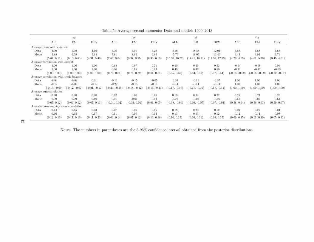
Table 5: Average second moments: Data and model: 1900–2013

gy gc gi tby

ALL EM DEV ALL EM DEV ALL EM DEV ALL EM DEV

Average Standard deviationData 4.90 5.39 4.19 6.30 7.01 5.28 16.25 18.58 12.91 4.68 4.68 4.68Model 5.88 6.39 5.15 7.81 8.65 6.62 15.75 18.05 12.46 4.43 4.93 3.71

(5.67, 6.11) (6.13, 6.68) (4.91, 5.40) (7.60, 8.04) (8.37, 8.95) (6.36, 6.88) (15.30, 16.22) (17.41, 18.71) (11.96, 12.99) (4.20, 4.69) (4.61, 5.30) (3.45, 4.01)Average correlation with output

Data 1.00 1.00 1.00 0.68 0.67 0.71 0.50 0.49 0.52 -0.04 -0.08 0.01Model 1.00 1.00 1.00 0.80 0.78 0.83 0.48 0.46 0.50 -0.11 -0.12 -0.09

(1.00, 1.00) (1.00, 1.00) (1.00, 1.00) (0.79, 0.81) (0.76, 0.79) (0.81, 0.84) (0.45, 0.50) (0.43, 0.49) (0.47, 0.54) (-0.13, -0.09) (-0.15, -0.09) (-0.12, -0.07)Average correlation with trade balance

Data -0.04 -0.08 0.01 -0.11 -0.15 -0.05 -0.09 -0.11 -0.07 1.00 1.00 1.00Model -0.12 -0.09 -0.19 -0.22 -0.15 -0.14 -0.14 -0.14 -0.14 1.00 1.00 1.00

(-0.15, -0.09) (-0.12, -0.07) (-0.21, -0.17) (-0.24, -0.19) (-0.18, -0.12) (-0.16, -0.11) (-0.17, -0.10) (-0.17, -0.10) (-0.17, -0.11) (1.00, 1.00) (1.00, 1.00) (1.00, 1.00)Average autocorrelation

Data 0.20 0.20 0.20 0.02 0.00 0.05 0.18 0.14 0.22 0.75 0.73 0.76Model 0.09 0.09 0.10 0.01 -0.01 0.03 -0.07 -0.09 -0.06 0.61 0.60 0.63

(0.07, 0.12) (0.06, 0.12) (0.07, 0.13) (-0.01, 0.02) (-0.03, 0.01) (0.01, 0.05) (-0.08, -0.06) (-0.10, -0.07) (-0.07, -0.04) (0.58, 0.64) (0.56, 0.63) (0.59, 0.67)Average cross country cross correlation

Data 0.14 0.15 0.23 0.07 0.06 0.15 0.18 0.20 0.19 0.09 0.21 0.04Model 0.16 0.15 0.17 0.11 0.10 0.14 0.13 0.13 0.12 0.12 0.14 0.08

(0.12, 0.19) (0.11, 0.19) (0.11, 0.23) (0.09, 0.14) (0.07, 0.12) (0.10, 0.18) (0.10, 0.15) (0.10, 0.16) (0.09, 0.15) (0.09, 0.15) (0.11, 0.19) (0.05, 0.11)

Notes: The numbers in parentheses are the 5-95% confidence interval obtained from the posterior distributions.

43

Table 6: Trend vs. stationary productivity shocks: 1900–2013

Country All trend All stationary Common trend Common stationary

Argentina 8.91 84.68 0.55 30.13Brazil 28.55 51.30 3.97 33.66Chile 9.22 82.02 4.54 30.94Colombia 4.71 56.51 1.16 16.11India 68.04 18.90 3.68 4.15Mexico 6.02 84.23 2.44 24.42Peru 37.47 55.68 5.05 46.86Taiwan 60.86 33.71 26.85 1.62Turkey 21.48 74.31 0.93 5.58Venezuela 63.62 29.47 4.52 23.51Australia 68.42 8.81 57.58 3.50Canada 55.95 37.65 5.87 31.85Finland 14.31 77.64 10.52 19.89Norway 13.61 75.31 4.67 14.57Portugal 78.00 13.50 1.60 4.06Spain 9.05 79.78 6.15 1.75Sweden 29.02 65.87 2.09 17.17

Average 33.96 54.67 8.36 18.22EM 30.89 57.08 5.37 21.70DEV 38.34 51.22 12.64 13.26

Notes: The table reports the means of the posterior distributions of the contributionof trend, stationary productivity shocks, and common trend and common stationaryproductivity shocks to output growth rates in each country.

44

Table 7: Contribution of common shocks to each country between 1900 and 2013: Average across countries

gy gc gi tby

All EM DEV All EM DEV All EM DEV All EM DEV

µ 8.36 5.37 12.64 5.17 3.66 7.32 3.07 2.50 3.89 0.97 1.14 0.74a 18.22 21.70 13.25 11.96 12.72 10.87 6.86 7.58 5.83 1.14 1.22 1.02pm 0.65 0.83 0.39 0.54 0.72 0.29 8.03 9.29 6.23 14.00 17.10 9.57b 0.97 1.13 0.75 3.36 3.39 3.31 2.77 2.93 2.55 4.77 5.40 3.88g 0.21 0.08 0.39 1.23 0.41 2.41 1.10 0.47 1.99 1.08 0.43 2.00

Total 28.42 29.11 27.43 22.26 20.90 24.19 21.82 22.76 20.49 21.96 25.28 17.22

Notes: All results are reported using the mean of variance decomposition computedfrom eight chains of 1 million draws each with half burn-in from the posterior distribu-tion. We take averages of the mean variance decomposition across all countries (ALL),developed countries (DEV) and developing countries (EM).

Table 8: Dynamic factor estimation

Output Consumption Investment TBY

Median 11.33 7.62 10.56 7.77

(8.19, 14.0) (5.36, 9.76) (5.99, 14.8) (3.13, 13.58)

Notes: Total contribution of common shocks to output, consumption, investment, andthe trade-balance-to-output ratio using actual data estimated by the DFM approach.The results are reported at the mean from the posterior distribution with 20,000 drawsand the parentheses are the 5% and 95% confidence interval.

Table 9: Subsample stability

Baseline 1901–1950 1951–2013EM DEV EM DEV EM DEV

φjD 1.04 0.75 1.29 0.65 0.57 0.86

φjSR 0.46 0.51 0.47 0.88 0.85 0.48Trend 30.39 38.34 30.20 45.58 35.90 32.74Stationary 57.08 51.22 60.01 50.30 54.24 52.13Common shocks 29.11 27.43 39.19 35.66 23.29 42.39

Notes: All results are reported using the mean of variance decomposition computedfrom eight chains of 1 million draws each with half burn-in from the posterior distri-bution. We take averages of the mean across all countries (ALL), developed countries(DEV) and developing countries (EM). φjD and φjSR are the mean of the estimated pa-rameters across countries. Trend, Stationary and Common shocks are the contributionof all trend shocks, all stationary shocks, and all common shocks to output fluctuationsin these countries, respectively.

45

Appendix B Additional Tables and Figures: Not for publication

Table A1: Data availability

Country Output Consumption Investment Trade balance

Argentina 1900–2012 1900–2012 1900–2012 1900–2012Brazil 1901–2013 1901–2013 1901–2013 1901–2013Chile 1900–2013 1900–2013 1900–2013 1900–2013Colombia 1925–2013 1925–2013 1925–2013 1925–2013India 1919–2013 1919–2013 1919–2013 1919–2013Mexico 1900–2013 1900–2013 1900–2013 1900–2013Peru 1900–2013 1900–2013 1900–2013 1900–2013Taiwan 1901–2013 1901–2013 1901–2013 1901–2013Turkey 1923–2013 1923–2013 1923–2013 1923–2013Venezuela 1920–2012 1920–2012 1920–2012 1920–2012Australia 1901–2013 1901–2013 1901–2013 1901–2013Canada 1900–2013 1900–2013 1900–2013 1900–2013Finland 1900–2013 1900–2013 1900–2013 1900–2013Norway 1900–2013 1900–2013 1900–2013 1900–2013Portugal 1910–2013 1910–2013 1910–2013 1910–2013Spain 1900–2013 1900–2013 1900–2013 1900–2013Sweden 1900–2013 1900–2013 1900–2013 1900–2013

46

Table A2: Cross-country correlations of output: 1900–2013

Arg Aus Bra Can Chile Col Fin Ind Mex Nor Peru Port Spain Swe Taiw Turk Vene

Arg 1.00 0.19 0.22 0.30 -0.01 0.27 0.36 0.05 0.13 0.38 0.17 0.10 0.14 0.06 0.12 0.08 0.19Aus 0.19 1.00 0.16 0.50 -0.25 0.19 0.36 0.10 0.07 0.20 0.16 0.21 0.42 0.25 0.21 0.03 0.25Bra 0.22 0.16 1.00 0.25 -0.03 0.17 0.29 0.00 0.26 0.20 0.22 0.28 0.01 0.07 0.00 0.00 0.07Can 0.30 0.50 0.25 1.00 -0.09 0.02 0.38 -0.01 0.17 0.48 -0.01 0.06 0.19 0.23 0.03 0.01 0.22Chile -0.01 -0.25 -0.03 -0.09 1.00 -0.15 0.02 0.14 -0.02 -0.21 0.13 -0.05 -0.15 -0.22 -0.17 0.00 -0.14Col 0.27 0.19 0.17 0.02 -0.15 1.00 0.24 0.09 0.18 0.06 0.22 0.18 0.18 -0.01 0.09 0.04 0.19Fin 0.36 0.36 0.29 0.38 0.02 0.24 1.00 0.00 0.22 0.32 0.13 0.23 0.14 0.10 -0.07 0.04 0.24Ind 0.05 0.10 0.00 -0.01 0.14 0.09 0.00 1.00 0.41 -0.12 0.32 0.10 0.16 0.03 0.23 0.23 0.13Mex 0.13 0.07 0.26 0.17 -0.02 0.18 0.22 0.41 1.00 0.20 -0.09 -0.05 0.08 0.17 -0.10 -0.10 0.35Nor 0.38 0.20 0.20 0.48 -0.21 0.06 0.32 -0.12 0.20 1.00 -0.15 0.16 0.12 0.29 0.02 -0.03 0.23Peru 0.17 0.16 0.22 -0.01 0.13 0.22 0.13 0.32 -0.09 -0.15 1.00 0.40 0.37 -0.01 0.11 0.12 0.06Port 0.10 0.21 0.28 0.06 -0.05 0.18 0.23 0.10 -0.05 0.16 0.40 1.00 0.11 0.11 0.07 0.19 0.27Spain 0.14 0.42 0.01 0.19 -0.15 0.18 0.14 0.16 0.08 0.12 0.37 0.11 1.00 0.44 0.34 0.19 0.48Swe 0.06 0.25 0.07 0.23 -0.22 -0.01 0.10 0.03 0.17 0.29 -0.01 0.11 0.44 1.00 0.17 0.02 0.60Taiw 0.12 0.21 0.00 0.03 -0.17 0.09 -0.07 0.23 -0.10 0.02 0.11 0.07 0.34 0.17 1.00 0.39 0.23Turk 0.08 0.03 0.00 0.01 0.00 0.04 0.04 0.23 -0.10 -0.03 0.12 0.19 0.19 0.02 0.39 1.00 0.12Vene 0.19 0.25 0.07 0.22 -0.14 0.19 0.24 0.13 0.35 0.23 0.06 0.27 0.48 0.60 0.23 0.12 1.00

47

Table A3: Output growth rates for 17 small open economies 1900 and 2013

year1910 1920 1930 1940 1950 1960 1970 1980 1990 2000 2010

grow

th r

ate

-0.7

-0.6

-0.5

-0.4

-0.3

-0.2

-0.1

0

0.1

0.2

Growth rate of real GDP 1900-2013

ArgentinaBrazilChileColombiaIndiaMexicoPeruTaiwanTurkeyVenezuelaAustraliaCanadaFinlandNorwayPortugalSpainSwedenmean

Note: Shaded regions are major historical events.

48

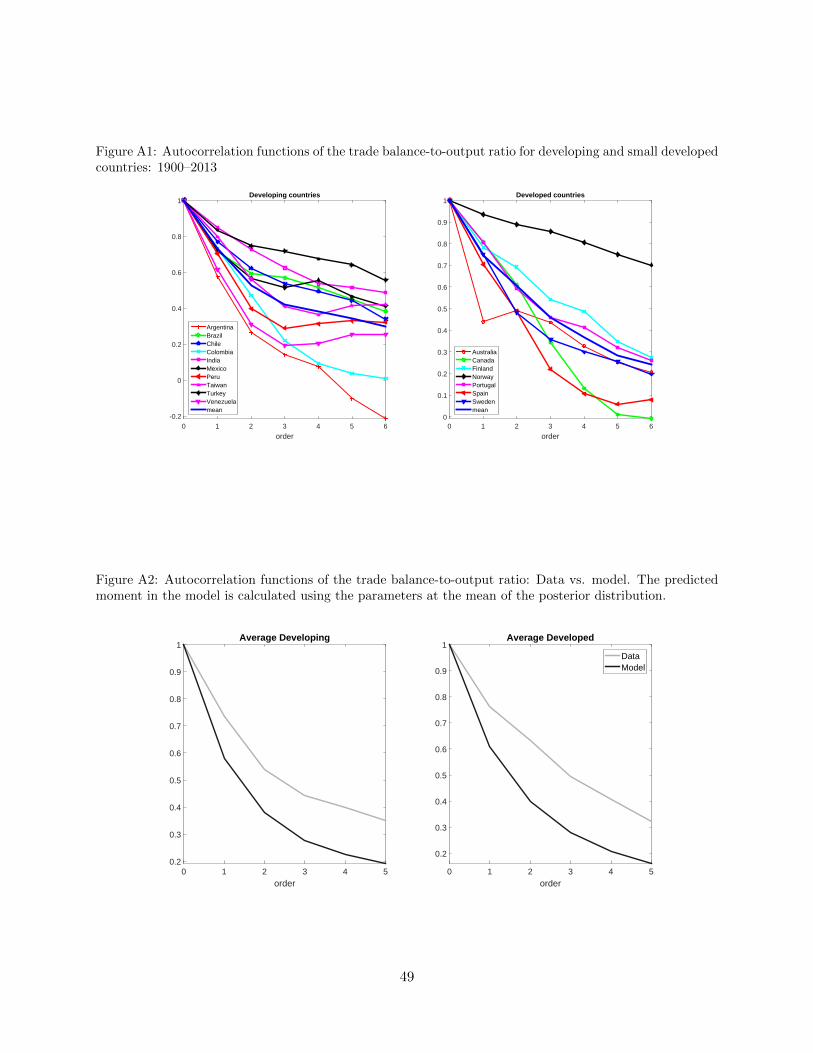
Figure A1: Autocorrelation functions of the trade balance-to-output ratio for developing and small developedcountries: 1900–2013

order0 1 2 3 4 5 6

-0.2

0

0.2

0.4

0.6

0.8

1Developing countries

ArgentinaBrazilChileColombiaIndiaMexicoPeruTaiwanTurkeyVenezuelamean

order0 1 2 3 4 5 6

0

0.1

0.2

0.3

0.4

0.5

0.6

0.7

0.8

0.9

1Developed countries

AustraliaCanadaFinlandNorwayPortugalSpainSwedenmean

Figure A2: Autocorrelation functions of the trade balance-to-output ratio: Data vs. model. The predictedmoment in the model is calculated using the parameters at the mean of the posterior distribution.

order0 1 2 3 4 5

0.2

0.3

0.4

0.5

0.6

0.7

0.8

0.9

1Average Developing

order0 1 2 3 4 5

0.2

0.3

0.4

0.5

0.6

0.7

0.8

0.9

1Average Developed

DataModel

49

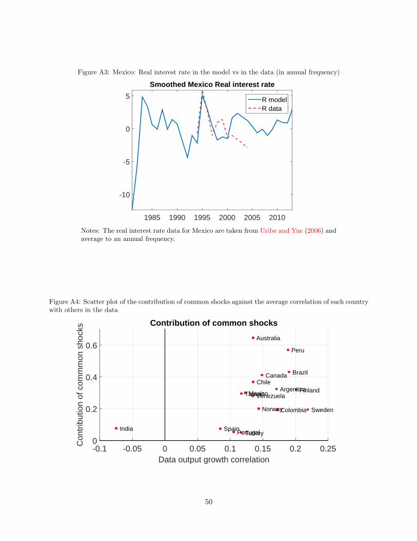
Figure A3: Mexico: Real interest rate in the model vs in the data (in annual frequency)

1985 1990 1995 2000 2005 2010

-10

-5

0

5

Smoothed Mexico Real interest rate

R modelR data

Notes: The real interest rate data for Mexico are taken from Uribe and Yue (2006) andaverage to an annual frequency.

Figure A4: Scatter plot of the contribution of common shocks against the average correlation of each countrywith others in the data

Data output growth correlation-0.1 -0.05 0 0.05 0.1 0.15 0.2 0.25

Con

trib

utio

n of

com

mm

on s

hock

s

0

0.2

0.4

0.6

Argentina

Brazil

Chile

Colombia

India

Mexico

Peru

Taiwan

Turkey

Venezuela

Australia

Canada

Finland

Norway

Portugal Spain

Sweden

Contribution of common shocks

50

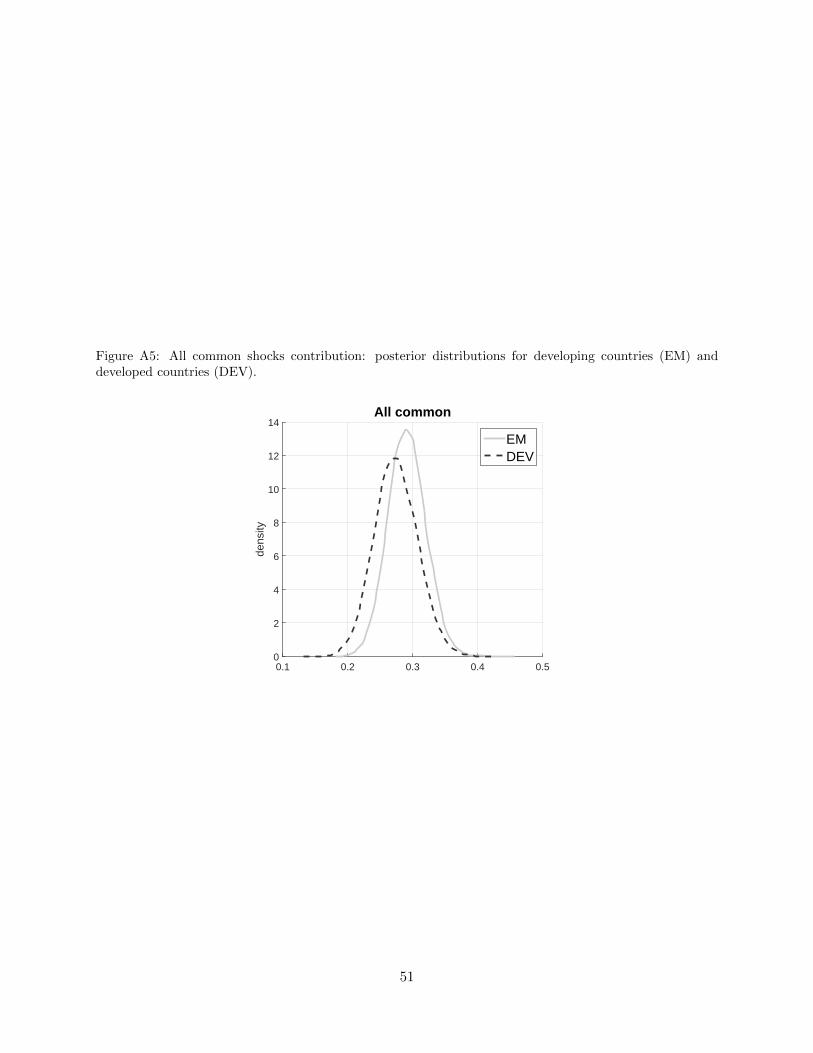
Figure A5: All common shocks contribution: posterior distributions for developing countries (EM) anddeveloped countries (DEV).

0.1 0.2 0.3 0.4 0.5

dens

ity

0

2

4

6

8

10

12

14All common

EMDEV

51

Appendix C Data Source

The data are compiled from many sources but primarily, as stated in the paper, from Barro and

Ursua (2009) data set for GDP per capita and consumption per capita. All population data are

taken from Maddison (2009). All updated data between 2007 and 2013 are from the International

Financial Statistics unless otherwise stated.

1. Argentina: Updated the data set given by Garcia-Cicco, Pancrazi and Uribe (2010) available

at http://www.columbia.edu/~mu2166/rbc_emerging/rbc_emerging.html

2006 data are from Secretearia de Politica Economica (2006). Available at http://www.

mecon.gov.ar/peconomica/informe/indice.htm and http://www.indec.gov.ar/principal.

asp?id_tema=165

2. Australia: GDP and Consumption per capita are taken from Barro and Ursua (2009) avail-

able at http://www.economics.harvard.edu/faculty/barro/data_sets_barro

Investment and Trade balance:

1901-1959: Vamplew, Wray (ed.), Australians, historical statistics, Fairfax, Syme & Weldon,

Australia, 1987.

1960-2006: Central bank Statistics available at http://abs.gov.au/AUSSTATS/[email protected]/

DetailsPage/5206.0Dec%202009?OpenDocument

3. Brazil: GDP and Consumption per capita are taken from Barro and Ursua (2009) as above


1900-2000: OxLad available at http://oxlad.qeh.ox.ac.uk/search.php

2001-2007: IFS available at http://www.imfstatistics.org/IMF/imfbrowser.aspx?branch=

ROOT

IPPEA available at http://www.ipeadata.gov.br/ipeaweb.dll/ipeadata?Tick=1356034625

and Estatısticas Economicas available at http://www.ibge.gov.br/seculoxx/economia/

contas_nacionais/contas_nacionais.shtm

4. Canada: GDP and Consumption per capita are taken from Barro and Ursua (2009) as above


52

http://www.columbia.edu/~mu2166/rbc_emerging/rbc_emerging.html

http://www.mecon.gov.ar/peconomica/informe/indice.htm

http://www.mecon.gov.ar/peconomica/informe/indice.htm

http://www.indec.gov.ar/principal.asp?id_tema=165

http://www.indec.gov.ar/principal.asp?id_tema=165

http://www.economics.harvard.edu/faculty/barro/data_sets_barro

http://abs.gov.au/AUSSTATS/[email protected]/DetailsPage/5206.0Dec%202009?OpenDocument

http://abs.gov.au/AUSSTATS/[email protected]/DetailsPage/5206.0Dec%202009?OpenDocument

http://oxlad.qeh.ox.ac.uk/search.php

http://www.imfstatistics.org/IMF/imfbrowser.aspx?branch=ROOT

http://www.imfstatistics.org/IMF/imfbrowser.aspx?branch=ROOT

http://www.ipeadata.gov.br/ipeaweb.dll/ipeadata?Tick=1356034625

http://www.ibge.gov.br/seculoxx/economia/contas_nacionais/contas_nacionais.shtm

http://www.ibge.gov.br/seculoxx/economia/contas_nacionais/contas_nacionais.shtm

1900-1925: Urquhart, M.C., Gross National Product, Canada, 1870-1926: The Derivation of

the Estimates, McGill-Queen’s University Press, Canada, 1993

1926-1960: Historical Statistics of Canada, 2nd edition. 1983, available at http://www.

statcan.gc.ca/pub/11-516-x/11-516-x1983001-eng.htm

1961-2006: Statistics Canada, National Income and Expenditure Accounts [Table 380-0017:

Gross Domestic Product (GDP), expenditure-based]. Available at: http://cansim2.statcan.

ca/

5. Chile: GDP and Consumption per capita are taken from Barro and Ursua (2009) as above


1900-1980: OxLad as above

1981-2006: IFS as above

Braun, Juan, Matıas Braun, Ignacio Briones, and Jose Dıaz, “Economıa Chilena 1810-1995:

Estadısticas Historicas”, Instituto de Economıa - Pontifica Universidad Catolica de Chile,

Documento de Trabajo No. 187, January, 2000.

6. Colombia: All data are taken from Fernandez, Andres. “Tropical” Real Business Cycles?

A Bayesian Exploration (2009). Mimeo, Rutgers University, and Banco de la Republica

Colombia, at http://www.banrep.gov.co/series-estadisticas/see_prod_salar.htm

7. Finland: GDP and Consumption per capita are taken from Barro and Ursua (2009) as above


1900-1975: Hjerppe, Riitta, The Finnish Economy 1860-1985: Growth and Structural Change,

Bank of Finland Publications, Studies on Finland’s Economic Growth XIII, Helsinki, 1989.

1975-2006: Statistics Finland, available at http://pxweb2.stat.fi/database/StatFin/

kan/pka/pka_en.asp

8. India: GDP and Consumption per capita are taken from Barro and Ursua (2009) as above


1919-1950: Narasinham, N. V. A., A Short Term Planning Model for India, North Holland

Publishing Company, Amsterdam, 1956.

53

http://www.statcan.gc.ca/pub/11-516-x/11-516-x1983001-eng.htm

http://www.statcan.gc.ca/pub/11-516-x/11-516-x1983001-eng.htm

http://cansim2.statcan.ca/

http://cansim2.statcan.ca/

http://www.banrep.gov.co/series-estadisticas/see_prod_salar.htm

http://pxweb2.stat.fi/database/StatFin/kan/pka/pka_en.asp

http://pxweb2.stat.fi/database/StatFin/kan/pka/pka_en.asp

1951-2006: Central Statistical Office, Government of India, “National Accounts tables”, avail-

able at http://mospi.nic.in/mospi_nad_main.htm

9. Mexico: I updated the data set given by Garcia-Cicco, Pancrazi and Uribe (2010). 2006

data are from Instituto Nacional de Estadıistica, Geografıia e Informatica (INEGI), available

at http://dgcnesyp.inegi.org.mx/bdiesi/bdie.html

10. Norway: All data are taken from:

1830-1969: Grytten, Ola, “The gross domestic product for Norway 1830–2003”, in: Øyvind

Eitrheim, Jan T. Klovland and Jan F. Qvigstad (eds.), Historical monetary statistics for

Norway, 2005. Available at the Nordic Historical National Accounts Database, (courtesy of

Guomundur Jonsson), available at http://old.nhh.no/forskning/nnb/

1941-1945: Ola Grytten kindly provided me with his estimates

1970-2006: Central Bank of Norway, “National accounts”, available at http://www.ssb.no/

english/subjects/09/01/nr_en/

11. Peru: GDP and Consumption per capita are taken from Barro and Ursua (2009) as above.

All other data are from courtesy of Bruno Seminario, available at http://sites.google.

com/site/lbseminario/peru-2021

12. Portugal: GDP and Consumption per capita are taken from Barro and Ursua (2009) as

above. All other data are taken from:

Batista, Dina; Martins, Carlos; Pinheiro, Maximiano and Reis, Jaime, New Estimates for

Portugal’s GDP (1910-1958), Lisboa, 1997. Available at Professor Pedro Lain’s personal

website http://pedrolains.typepad.com/pedrolains/estatsticas-data.html

13. Spain: GDP and Consumption per capita are taken from Barro and Ursua (2009) as above.

Additionally, data are taken from

1900-1994: Prados de la Escosura, Leandro, El progreso economico de Espana, 1850-2000,

Fundacion BBVA, Madrid, 2003

1995-2006: Instituto Nacional de Estadıstica, Contabilidad Nacional de Espana, Producto

interior bruto a precios de mercado y sus componentes http://www.ine.es/jaxi/menu.do?

L=1&type=pcaxis&path=%2Ft35%2Fp008&file=inebase&N=&L=

54

http://mospi.nic.in/mospi_nad_main.htm

http://dgcnesyp.inegi.org.mx/bdiesi/bdie.html

http://old.nhh.no/forskning/nnb/

http://www.ssb.no/english/subjects/09/01/nr_en/

http://www.ssb.no/english/subjects/09/01/nr_en/

http://sites.google.com/site/lbseminario/peru-2021

http://sites.google.com/site/lbseminario/peru-2021

http://pedrolains.typepad.com/pedrolains/estatsticas-data.html

http://www.ine.es/jaxi/menu.do?L=1&type=pcaxis&path=%2Ft35%2Fp008&file=inebase&N=&L=

http://www.ine.es/jaxi/menu.do?L=1&type=pcaxis&path=%2Ft35%2Fp008&file=inebase&N=&L=

14. Sweden: GDP and Consumption per capita are taken from Barro and Ursua (2009) as above.


Edvinsson, Rodney, Historical national accounts for Sweden 1800-2000 (Historiskanation-

alrakenskaper for Sverige 1800-2000). Based on:Edvinsson, R., 2005: Growth, Accumulation,

Crisis: With New Macroeconomic Data for Sweden. Almqvist & Wiksell International; Stock-

holm.

1900-1992: the Nordic Historical National Accounts Database, available at http://old.nhh.

no/forskning/nnb/

1993-2006: Statistics Sweden, Economic statistics available at http://www.scb.se/Pages/

List____258713.aspx

15. Taiwan: GDP and Consumption per capita are taken from Barro and Ursua (2009) as above.


1901-1950: National Historical data

Mizoguchi, Toshiyuki, “Estimates of the Long-run Economic Growth of Taiwan Based on Re-

vised SNA (1901-2000) Statistics”, Institute for Economic Research - Hitotsubashi University,

Discussion Paper Series, No. 123, October, 2005.

1951-2013: National statistics, available at http://eng.stat.gov.tw/mp.asp?mp=5

16. Turkey: GDP and Consumption per capita are taken from Barro and Ursua (2009) as above.


Altug, Sumru, Alpay Filitztekin and Sevket Pamuk. “Sources of long-term economic growth

for Turkey, 1880-2005”. European Review of Economic History, 12(3) pp.393-430, December

2008. Available at http://myweb.sabanciuniv.edu/alpayf/my-research/data/

Turkish Statistical Institute. Foreign Trade table, available at http://www.turkstat.gov.

tr/PreTablo.do?tb_id=12&ust_id=4

State Institute of Statistics (Devlet Istatistik Enstitusu), Statistical indicators (Istatistik

gostergeler): 1923-2008, Ankara, Turkey, 2009, available at http://www.tuik.gov.tr/Kitap.

do?metod=KitapDetay&KT_ID=0&KITAP_ID=158

17. Venezuela: Besides data taken from Barro and Ursua (2009) as above, I also constructed

GDP, Consumption per capita and the other series from:

55



http://www.scb.se/Pages/List____258713.aspx

http://www.scb.se/Pages/List____258713.aspx

http://eng.stat.gov.tw/mp.asp?mp=5

http://myweb.sabanciuniv.edu/alpayf/my-research/data/

http://www.turkstat.gov.tr/PreTablo.do?tb_id=12&ust_id=4

http://www.turkstat.gov.tr/PreTablo.do?tb_id=12&ust_id=4

http://www.tuik.gov.tr/Kitap.do?metod=KitapDetay&KT_ID=0&KITAP_ID=158

http://www.tuik.gov.tr/Kitap.do?metod=KitapDetay&KT_ID=0&KITAP_ID=158

1920-2002: Baptista, Asdrubal, Bases Cuantitativas de la Economıa Venezolana: 1830-2002,

Fundacion Polar, Caracas, Venezuela, 2006

1998-2006: Central bank of Venezuela: Banco Central De Venezuela, available at http:

//www.bcv.org.ve/c2/indicadores.asp

56

http://www.bcv.org.ve/c2/indicadores.asp

http://www.bcv.org.ve/c2/indicadores.asp

Business Cycles in Small, Open Economies: Evidence from ...€¦ · Bank of Canada Staff Working...

Documents

Transcript of Business Cycles in Small, Open Economies: Evidence from ...€¦ · Bank of Canada Staff Working...