
Reducedorder modeling based on POD of a parabolized ...inavon/pubs/fld2606.pdf · 4School of...
21
INTERNATIONAL JOURNAL FOR NUMERICAL METHODS IN FLUIDS Int. J. Numer. Meth. Fluids 2012; 69:710–730 Published online 1 June 2011 in Wiley Online Library (wileyonlinelibrary.com ). DOI: 10.1002/fld.2606 Reduced-order modeling based on POD of a parabolized Navier–Stokes equation model I: forward model J. Du 1,2 , I. M. Navon 2, * ,† , J. L. Steward 2 , A. K. Alekseev 3 and Z. Luo 4 1 School of Science, Beijing Jiaotong University, Beijing 100044, China 2 Department of Scientific Computing, Florida State University, Tallahassee, FL 32306-4120, USA 3 Moscow Institute of Physics and Technology, Moscow 141700, Russia 4 School of Mathematics and Physics, North China Electric Power University, Beijing 102206, China SUMMARY A proper orthogonal decomposition (POD)-based reduced-order model of the parabolized Navier–Stokes (PNS) equations is derived in this article. A space-marching finite difference method with time relaxation is used to obtain the solution of this problem, from which snapshots are obtained to generate the POD basis functions used to construct the reduced-order model. In order to improve the accuracy and the stability of the reduced-order model in the presence of a high Reynolds number, we applied a Sobolev H 1 norm calibration to the POD construction process. Finally, some numerical tests with a high-fidelity model as well as the POD reduced-order model were carried out to demonstrate the efficiency and the accuracy of the reduced-order model for solving the PNS equations compared with the full PNS model. Different inflow conditions and dif- ferent selections of snapshots were experimented to test the POD reduction technique. The efficiency of the H 1 norm POD calibration is illustrated for the PNS model with increasingly higher Reynolds numbers, along with the optimal dissipation coefficient derivation, yielding the best root mean square error and correlation coefficient between the full and reduced-order PNS models. Copyright © 2011 John Wiley & Sons, Ltd. Received 21 July 2010; Revised 6 March 2011; Accepted 12 April 2011 KEY WORDS: parabolized Navier–Stokes (PNS); proper orthogonal decomposition (POD); H 1 norm POD calibration; correlation coefficient; optimal dissipation coefficient; high Reynolds number 1. INTRODUCTION For steady two-dimensional or three-dimensional flow, the complete Navier–Stokes equations can be simplified by eliminating some specific terms to provide detailed flow descriptions for large Reynolds number flows. If second-order viscous terms are eliminated and only convection and pres- sure gradient terms are retained, we can obtain the inviscid equations (Euler equation). If only the streamwise second-order viscous terms (i.e. in the x direction along the surface, downstream direction) are eliminated, we can obtain the so-called parabolized Navier–Stokes (PNS) equations. The PNS equations are mathematically a set of mixed hyperbolic–parabolic equations along the assumed local streamwise flow direction, which can be used to predict complex three-dimensional steady, supersonic, viscous flow fields in an efficient manner. These types of equations satisfy cer- tain conditions based on the coefficients of the terms in the equations and also accepts one real solution in the streamwise direction. The efficiency of the PNS equations is achieved because of the fact that the equations can be solved using a space-marching finite difference technique as opposed to the time-marching technique, which is normally employed for the complete Navier–Stokes equa- tions. In these simplified equations, just like in the boundary layer equations, one can obtain the *Correspondence to: I. M. Navon, Department of Scientific Computing, Florida State University, Tallahassee, FL 32306-4120, USA. † E-mail: [email protected] Copyright © 2011 John Wiley & Sons, Ltd. /journal/nmf
Transcript of Reducedorder modeling based on POD of a parabolized ...inavon/pubs/fld2606.pdf · 4School of...

INTERNATIONAL JOURNAL FOR NUMERICAL METHODS IN FLUIDSInt. J. Numer. Meth. Fluids 2012; 69:710–730Published online 1 June 2011 in Wiley Online Library (wileyonlinelibrary.com ). DOI: 10.1002/fld.2606
Reduced-order modeling based on POD of a parabolizedNavier–Stokes equation model I: forward model
J. Du1,2, I. M. Navon2,*,†, J. L. Steward2, A. K. Alekseev3 and Z. Luo4
1School of Science, Beijing Jiaotong University, Beijing 100044, China2Department of Scientific Computing, Florida State University, Tallahassee, FL 32306-4120, USA
3Moscow Institute of Physics and Technology, Moscow 141700, Russia4School of Mathematics and Physics, North China Electric Power University, Beijing 102206, China
SUMMARY
A proper orthogonal decomposition (POD)-based reduced-order model of the parabolized Navier–Stokes(PNS) equations is derived in this article. A space-marching finite difference method with time relaxation isused to obtain the solution of this problem, from which snapshots are obtained to generate the POD basisfunctions used to construct the reduced-order model. In order to improve the accuracy and the stability of thereduced-order model in the presence of a high Reynolds number, we applied a SobolevH1 norm calibrationto the POD construction process. Finally, some numerical tests with a high-fidelity model as well as the PODreduced-order model were carried out to demonstrate the efficiency and the accuracy of the reduced-ordermodel for solving the PNS equations compared with the full PNS model. Different inflow conditions and dif-ferent selections of snapshots were experimented to test the POD reduction technique. The efficiency of theH1 norm POD calibration is illustrated for the PNS model with increasingly higher Reynolds numbers, alongwith the optimal dissipation coefficient derivation, yielding the best root mean square error and correlationcoefficient between the full and reduced-order PNS models. Copyright © 2011 John Wiley & Sons, Ltd.
Received 21 July 2010; Revised 6 March 2011; Accepted 12 April 2011
KEY WORDS: parabolized Navier–Stokes (PNS); proper orthogonal decomposition (POD);H1 norm PODcalibration; correlation coefficient; optimal dissipation coefficient; high Reynolds number
1. INTRODUCTION
For steady two-dimensional or three-dimensional flow, the complete Navier–Stokes equations canbe simplified by eliminating some specific terms to provide detailed flow descriptions for largeReynolds number flows. If second-order viscous terms are eliminated and only convection and pres-sure gradient terms are retained, we can obtain the inviscid equations (Euler equation). If onlythe streamwise second-order viscous terms (i.e. in the x direction along the surface, downstreamdirection) are eliminated, we can obtain the so-called parabolized Navier–Stokes (PNS) equations.
The PNS equations are mathematically a set of mixed hyperbolic–parabolic equations along theassumed local streamwise flow direction, which can be used to predict complex three-dimensionalsteady, supersonic, viscous flow fields in an efficient manner. These types of equations satisfy cer-tain conditions based on the coefficients of the terms in the equations and also accepts one realsolution in the streamwise direction. The efficiency of the PNS equations is achieved because of thefact that the equations can be solved using a space-marching finite difference technique as opposedto the time-marching technique, which is normally employed for the complete Navier–Stokes equa-tions. In these simplified equations, just like in the boundary layer equations, one can obtain the
*Correspondence to: I. M. Navon, Department of Scientific Computing, Florida State University, Tallahassee, FL32306-4120, USA.
†E-mail: [email protected]
Copyright © 2011 John Wiley & Sons, Ltd.
/journal/nmf
REDUCED-ORDER MODELING BASED ON POD OF A PNS EQUATION MODEL 711
solution by marching in the streamwise direction (i.e. the x direction) from some known initial loca-tion. This is possible because the streamwise momentum equation (i.e. the x-momentum equation)has only first-order terms in the streamwise direction with the second-order viscous terms havingbeen already eliminated. The PNS equations can propagate the information only in the downstreamdirection; thus, they are not suitable for general flow situations, especially flows with separation.
Proper orthogonal decomposition (POD), also known as Karhunen–Loeve expansions in signalanalysis and pattern recognition [1], or principal component analysis in statistics [2], or the methodof empirical orthogonal functions in geophysical fluid dynamics [3] or meteorology [4], is a modelreduction technique offering adequate approximation for representing fluid flows with a reducednumber of degrees of freedom, that is, with lower-dimensional models [5–7]. The POD methodchanges the complex partial differential equations to a set of much simpler ordinary differentialequations of an efficiently reduced order so as to alleviate both the computational load and thememory requirements.
Because of the truncation applied in the POD reduced-order space, there is some information ofthe state variables missing in the POD reduced-order model. This neglected information has a veryimportant impact on the efficiency and the stability of the POD reduced-order model for flows withhigh Reynolds number (e.g. 103) as is our case. To improve the accuracy and the long-term stabilityof the POD reduced-order model, Galerkin projection is insufficient and numerical stabilization isrequired. This is provided by an artificial dissipation that is introduced using the Sobolev H1 innerproduct norm to calibrate the POD method.
In the present article, we apply the POD method to derive a reduced-order model of the PNS equa-tions and introduce an H1 norm POD calibration to solve the reduced-order model more robustly.The feasibility of the POD reduced-order model compared with the full PNS model and the effi-ciency of theH1 norm POD calibration in the presence of high Reynolds number are both analyzed.Because the PNS equations are already simplified Navier–Stokes equations, the POD reduced-ordermodeling applied to the PNS equations will yield a double benefit, namely the POD model reduc-tion as well as the simplification of the PNS equations. To the best of our knowledge, this is a newcontribution and the first application of POD reduced-order modeling to the PNS equations.
The present paper is organized as follows. Section 2 presents the specific model description of thePNS equations and the space-marching finite difference scheme with time relaxation to be used here.Section 3 provides the construction process of the POD reduced-order model, consisting of Sec-tion 3.1, where the basic theory of the POD method is provided, and Section 3.2, which illustratesthe process of applying the POD method to the PNS equations to obtain the POD reduced model,which are a set of ordinary differential equations of the POD coefficients. Section 4 presents theSobolev H1 inner product norm calibration being applied to the POD construction process in orderto enhance dissipation and increase the relevance of small-scale information in the POD reduced-order model for a high Reynolds number case. In Section 5, we present numerical results, whichdemonstrate the efficiency of the reduced-order method for solving the PNS equations comparedwith the full PNS model, using the POD reduced-order model. Different inflow conditions and dif-ferent numbers of snapshots are experimented to test the POD reduction technique. The efficiencyof the Sobolev H1 norm POD calibration in the presence of increasingly higher Reynolds numbersis also demonstrated using a numerically derived optimal dissipation coefficient. In Section 6, thesummary and conclusions are provided, including a discussion related to future research work.
2. PNS MODEL DESCRIPTION
For the PNS equations, the streamwise momentum equation (i.e. the x-momentum equation) hasonly first-order terms in the streamwise direction with the second-order viscous terms having beenalready eliminated. The PNS equations can propagate the information only in the downstreamdirection; thus, they are not suitable for general flow situations, especially flows with separation.However, the PNS equations have been applied successfully for a variety of two-dimensional andthree-dimensional supersonic flows, even with real gas effects, such as compressible hypersonicflows and flows with upstream influences due to strong shock interactions and confined regions ofreverse flow.
Copyright © 2011 John Wiley & Sons, Ltd. Int. J. Numer. Meth. Fluids 2012; 69:710–730DOI: 10.1002/fld
712 J. DU ET AL.
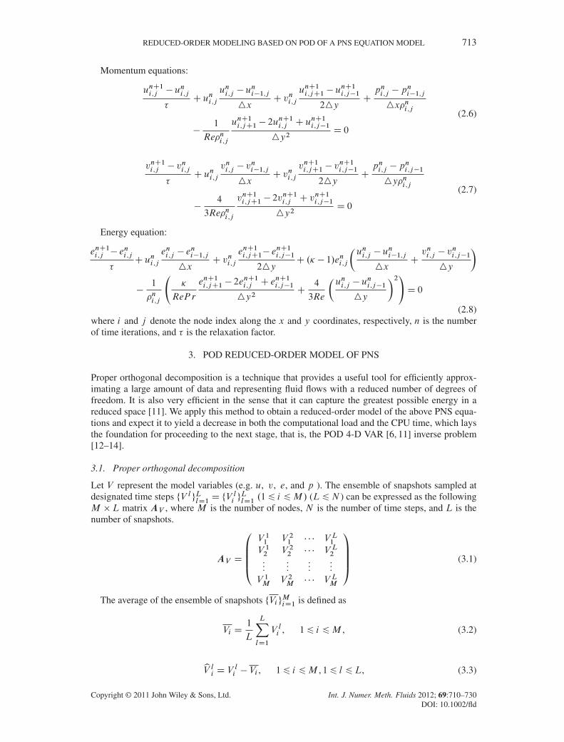
In this paper, the two-dimensional steady supersonic laminar flow is modeled by the PNS equa-tions [8]. This model is valid if the flow is supersonic along the x coordinate, and the second-orderviscous effects along this direction are negligible, a fact that allows a rapid decrease in the com-putational time required to complete the calculation [9]. The following equations describe anunder-expanded jet (Figure 1) in this flow.
8̂̂̂̂ˆ̂̂̂<̂ˆ̂̂̂̂̂̂:
@.�u/@xC @.�v/
@yD 0,
u @u@xC v @u
@yC 1
�@p@xD 1
Re�@2u@y2
,
u @v@xC v @v
@yC 1
�@p@yD 4
3Re�@2v@y2
,
u @e@xC v @e
@yC .� � 1/e
�@u@xC @v
@y
�D 1
�
��
ReP r@2e@y2C 4
3Re
�@u@y
�2�,
p D �RT , e D CvT D R.��1/T
, .x,y/ 2�D .0 < x < xmax, 0 < y < 1/,
(2.1)
where u and v represent the velocity components along the x and y directions, respectively, � repre-sents the flow density, p the pressure, e the specific energy,R the gas constant, T the temperature,Cv
the specific volume heat capacity, and � the specific heat ratio. Besides, Re D .�1u1ymax/=.�1/
is the Reynolds number, where1 indicates the inflow boundary parameter, ymax is the length of theflow field in the y direction, and � represents viscosity.
The following conditions are used for the inflow boundary (see A in Figure 1):
�.0, y/D �1.y/, u.0,y/D u1.y/, v.0,y/D v1.y/, e.0, y/D e1.y/, (2.2)
where �1.y/, u1.y/, v1.y/, and e1.y/ are all given functions.The lateral boundary (see B and C in Figure 1) conditions are prescribed as follows:
@�.x,y/
@yjyD0 D 0,
@u.x,y/
@yjyD0 D 0,
@v.x,y/
@yjyD0 D 0,
@e.x,y/
@yjyD0 D 0, (2.3)
@�.x,y/
@yjyD1 D 0,
@u.x,y/
@yjyD1 D 0,
@v.x,y/
@yjyD1 D 0,
@e.x,y/
@yjyD1 D 0. (2.4)
A space-marching finite difference discretization [10] is employed in Equations (2.5)–(2.8) toderive the solution of this problem. The finite difference discretization is of second-order accuracyin the y direction and of first order in the x direction. At every step along the x coordinate, the flowparameters are calculated from the initial inflow location in an iterative manner assuming the formof time relaxation.
Continuity equation:
�nC1i ,j � �ni ,j
�Cuni ,j
�ni ,j � �ni�1,j
4xCvni ,j
�nC1i ,jC1 � �nC1i ,j�1
24yC�ni ,j
�uni ,j � u
ni�1,j
4xCvni ,j � v
ni ,j�1
4y
�D 0
(2.5)
Figure 1. Flow region. A, inflow boundary; B and C, lateral boundaries; D, outflow boundary(measurement).
Copyright © 2011 John Wiley & Sons, Ltd. Int. J. Numer. Meth. Fluids 2012; 69:710–730DOI: 10.1002/fld
REDUCED-ORDER MODELING BASED ON POD OF A PNS EQUATION MODEL 713
Momentum equations:
unC1i ,j � uni ,j
�C uni ,j
uni ,j � uni�1,j
4xC vni ,j
unC1i ,jC1 � unC1i ,j�1
24yCpni ,j � p
ni�1,j
4x�ni ,j
�1
Re�ni ,j
unC1i ,jC1 � 2unC1i ,j C u
nC1i ,j�1
4y2D 0
(2.6)
vnC1i ,j � vni ,j
�C uni ,j
vni ,j � vni�1,j
4xC vni ,j
vnC1i ,jC1 � vnC1i ,j�1
24yCpni ,j � p
ni ,j�1
4y�ni ,j
�4
3Re�ni ,j
vnC1i ,jC1 � 2vnC1i ,j C v
nC1i ,j�1
4y2D 0
(2.7)
Energy equation:
enC1i ,j � eni ,j
�C uni ,j
eni ,j � eni�1,j
4xC vni ,j
enC1i ,jC1� enC1i ,j�1
24yC .� � 1/eni ,j
�uni ,j � u
ni�1,j
4xCvni ,j � v
ni ,j�1
4y
��
1
�ni ,j
�
ReP r
enC1i ,jC1 � 2enC1i ,j C e
nC1i ,j�1
4y2C
4
3Re
�uni ,j � u
ni ,j�1
4y
�2!D 0
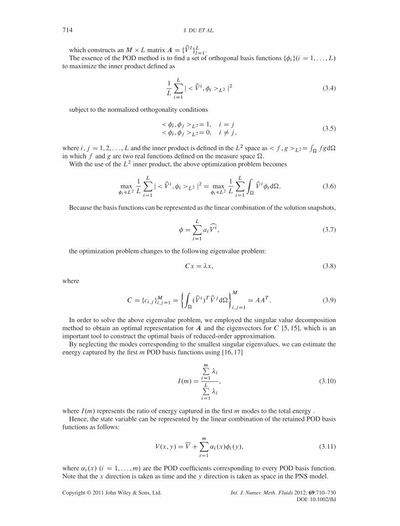
(2.8)where i and j denote the node index along the x and y coordinates, respectively, n is the numberof time iterations, and � is the relaxation factor.
3. POD REDUCED-ORDER MODEL OF PNS
Proper orthogonal decomposition is a technique that provides a useful tool for efficiently approx-imating a large amount of data and representing fluid flows with a reduced number of degrees offreedom. It is also very efficient in the sense that it can capture the greatest possible energy in areduced space [11]. We apply this method to obtain a reduced-order model of the above PNS equa-tions and expect it to yield a decrease in both the computational load and the CPU time, which laysthe foundation for proceeding to the next stage, that is, the POD 4-D VAR [6, 11] inverse problem[12–14].
3.1. Proper orthogonal decomposition
Let V represent the model variables (e.g. u, v, e, and p ). The ensemble of snapshots sampled atdesignated time steps ¹V lºL
lD1D ¹V li º
LlD1
.16 i 6M/ (L6N ) can be expressed as the followingM �L matrix AV , where M is the number of nodes, N is the number of time steps, and L is thenumber of snapshots.
AV D
0BBB@V 11 V 21 � � � V L1V 12 V 22 � � � V L2
......
......
V 1M V 2M � � � V LM
1CCCA (3.1)
The average of the ensemble of snapshots ¹ViºMiD1 is defined as
Vi D1
L
LXlD1
V li , 16 i 6M , (3.2)
bV li D V li � Vi , 16 i 6M , 16 l 6 L, (3.3)
Copyright © 2011 John Wiley & Sons, Ltd. Int. J. Numer. Meth. Fluids 2012; 69:710–730DOI: 10.1002/fld
714 J. DU ET AL.
which constructs an M �L matrix A D ¹bV lºLlD1
.The essence of the POD method is to find a set of orthogonal basis functions ¹�iº.i D 1, : : : ,L/
to maximize the inner product defined as
1
L
LXiD1
j< bV i ,�i >L2 j2 (3.4)
subject to the normalized orthogonality conditions
< �i ,�j >L2D 1, i D j< �i ,�j >L2D 0, i ¤ j ,
(3.5)
where i , j D 1, 2, : : : ,L and the inner product is defined in the L2 space as< f ,g >L2DR� fgd�
in which f and g are two real functions defined on the measure space �.With the use of the L2 inner product, the above optimization problem becomes
max�i2L
2
1
L
LXiD1
j< bV i ,�i >L2 j2 D max�i2L
2
1
L
LXiD1
Z�
bV i�id�. (3.6)
Because the basis functions can be represented as the linear combination of the solution snapshots,
� D
LXiD1
aicV i , (3.7)
the optimization problem changes to the following eigenvalue problem:
Cx D �x, (3.8)
where
C D ¹ci ,j ºMi ,jD1 D
²Z�
.bV i /TbV j d�
³Mi ,jD1
D AAT . (3.9)
In order to solve the above eigenvalue problem, we employed the singular value decompositionmethod to obtain an optimal representation for A and the eigenvectors for C [5, 15], which is animportant tool to construct the optimal basis of reduced-order approximation.
By neglecting the modes corresponding to the smallest singular eigenvalues, we can estimate theenergy captured by the first m POD basis functions using [16, 17]
I.m/D
mPiD1
�i
LPiD1
�i
, (3.10)
where I.m/ represents the ratio of energy captured in the first m modes to the total energy .Hence, the state variable can be represented by the linear combination of the retained POD basis
functions as follows:
V.x,y/D V CmXiD1
˛i .x/�i .y/, (3.11)
where ˛i .x/ .i D 1, : : : ,m/ are the POD coefficients corresponding to every POD basis function.Note that the x direction is taken as time and the y direction is taken as space in the PNS model.
Copyright © 2011 John Wiley & Sons, Ltd. Int. J. Numer. Meth. Fluids 2012; 69:710–730DOI: 10.1002/fld
REDUCED-ORDER MODELING BASED ON POD OF A PNS EQUATION MODEL 715
3.2. POD reduced model
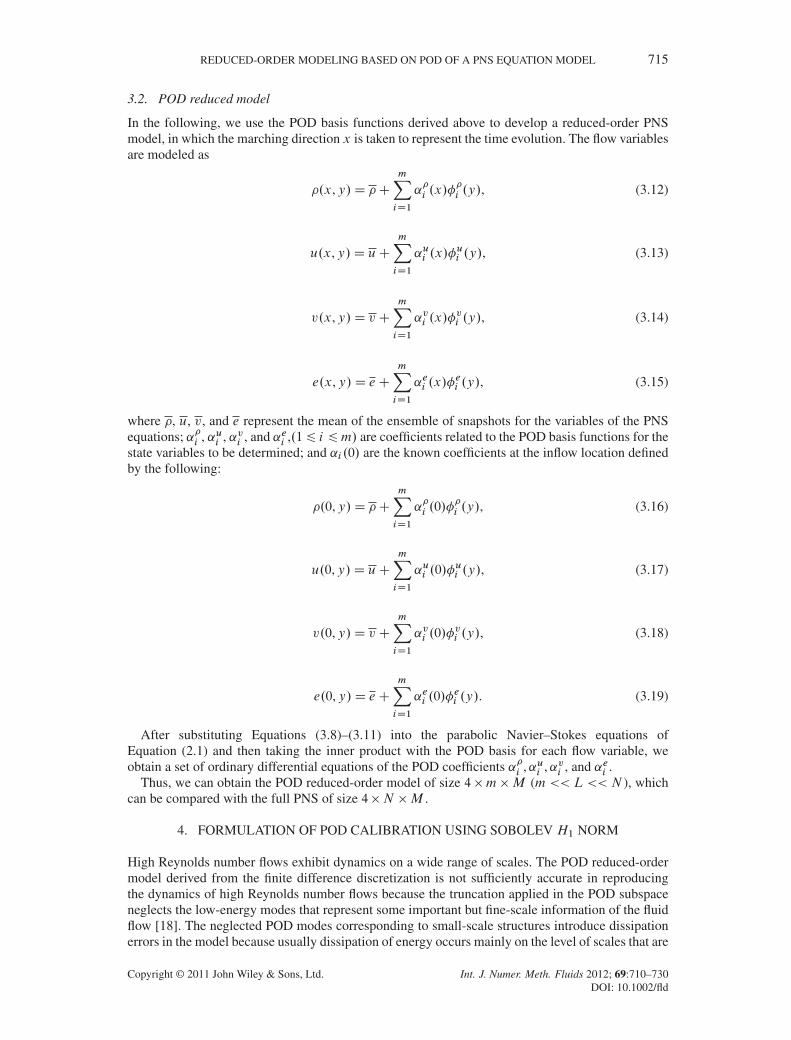
In the following, we use the POD basis functions derived above to develop a reduced-order PNSmodel, in which the marching direction x is taken to represent the time evolution. The flow variablesare modeled as
�.x,y/D �CmXiD1
˛�i .x/�
�i .y/, (3.12)
u.x,y/D uCmXiD1
˛ui .x/�ui .y/, (3.13)
v.x,y/D vCmXiD1
˛vi .x/�vi .y/, (3.14)
e.x,y/D eCmXiD1
˛ei .x/�ei .y/, (3.15)
where �, u, v, and e represent the mean of the ensemble of snapshots for the variables of the PNSequations; ˛�i , ˛ui , ˛vi , and ˛ei ,.16 i 6m/ are coefficients related to the POD basis functions for thestate variables to be determined; and ˛i .0/ are the known coefficients at the inflow location definedby the following:
�.0,y/D �CmXiD1
˛�i .0/�
�i .y/, (3.16)
u.0,y/D uCmXiD1
˛ui .0/�ui .y/, (3.17)
v.0,y/D vCmXiD1
˛vi .0/�vi .y/, (3.18)
e.0,y/D eCmXiD1
˛ei .0/�ei .y/. (3.19)
After substituting Equations (3.8)–(3.11) into the parabolic Navier–Stokes equations ofEquation (2.1) and then taking the inner product with the POD basis for each flow variable, weobtain a set of ordinary differential equations of the POD coefficients ˛�i ,˛ui ,˛vi , and ˛ei .
Thus, we can obtain the POD reduced-order model of size 4�m �M (m << L << N ), whichcan be compared with the full PNS of size 4�N �M .
4. FORMULATION OF POD CALIBRATION USING SOBOLEV H1 NORM
High Reynolds number flows exhibit dynamics on a wide range of scales. The POD reduced-ordermodel derived from the finite difference discretization is not sufficiently accurate in reproducingthe dynamics of high Reynolds number flows because the truncation applied in the POD subspaceneglects the low-energy modes that represent some important but fine-scale information of the fluidflow [18]. The neglected POD modes corresponding to small-scale structures introduce dissipationerrors in the model because usually dissipation of energy occurs mainly on the level of scales that are
Copyright © 2011 John Wiley & Sons, Ltd. Int. J. Numer. Meth. Fluids 2012; 69:710–730DOI: 10.1002/fld

716 J. DU ET AL.
unresolved in the discretization [19]. Consequently, the dynamic system may lose its long-term sta-bility. To ensure that the smaller scales are retained in the POD model and enhance dissipation, weintroduced an artificial dissipation by using a Sobolev H1 inner product norm to calibrate the PODmethod, that is, the derivatives of the snapshots and those of the basis functions are both included inthe formulation of the optimization problem [20].
Thus, the optimization problem in this calibrated POD process consists in seeking the POD basisfunctions �i , i D 1, : : : ,L to maximize
1
L
LXiD1
.< A,�i >/2 D
1
L
LXiD1
Z�
A�id�C Z�
rAr�id� (4.1)
subject to
< �i ,�j >H1D 1, i D j< �i ,�j >H1D 0, i ¤ j ,
(4.2)
where i , j D 1, : : : ,L.The corresponding eigenvalue problem becomes
Cx D �x, (4.3)
Figure 2. The initial condition for the specific energy e at the inflow boundary A (see Figure 1).
(a) (b)
Figure 3. The (a) first and (b) second POD basis functions of the specific energy e.
Copyright © 2011 John Wiley & Sons, Ltd. Int. J. Numer. Meth. Fluids 2012; 69:710–730DOI: 10.1002/fld
REDUCED-ORDER MODELING BASED ON POD OF A PNS EQUATION MODEL 717
(a) Leading SVD eigenvalues corresponding to the specific energy e
(c) Leading SVD eigenvalues of the x componentof the velocity field
(d) Leading SVD eigenvalues of the y componentof the velocity field
(b) Leading SVD eigenvalues corresponding to thedensity
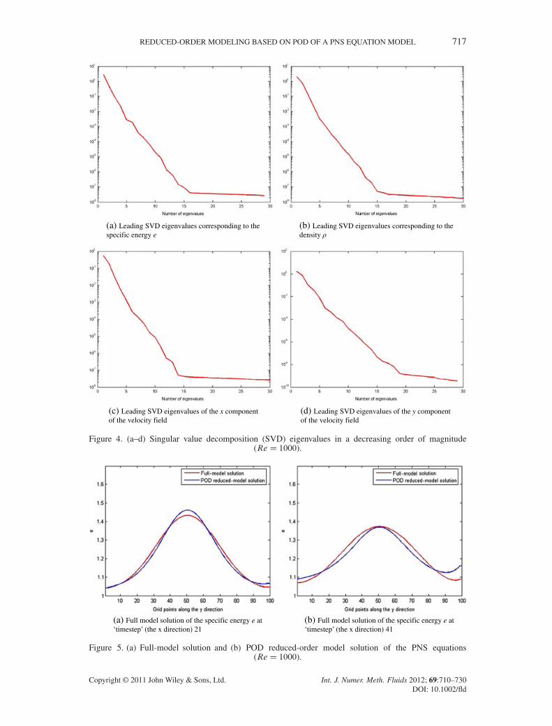
Figure 4. (a–d) Singular value decomposition (SVD) eigenvalues in a decreasing order of magnitude(Re D 1000).
(a) Full model solution of the specific energy e at‘timestep’ (the x direction) 21
(b) Full model solution of the specific energy e at‘timestep’ (the x direction) 41
Figure 5. (a) Full-model solution and (b) POD reduced-order model solution of the PNS equations(Re D 1000).
Copyright © 2011 John Wiley & Sons, Ltd. Int. J. Numer. Meth. Fluids 2012; 69:710–730DOI: 10.1002/fld

718 J. DU ET AL.
where
C D ¹ci ,j ºMi ,jD1 D
²Z�
.bV i /TbV j d�C
�Z�
r.bV i /TrbV j d�
�³Mi ,jD1
D AAT CrArAT ,
(4.4)
where is the dissipation coefficient whose value can be guessed to be proportional to T=Re becauseof dimensional analysis considerations, where T is some appropriate timescale [20].
5. NUMERICAL RESULTS
In this section, the flow field is computed by marching along the x coordinate, which representsthe time evolution from x D 0 to x D xmax. The computational grid contains 50–100 points in themarching direction (the x direction) and 100 points in the transversal direction (the y direction).We experimented with different Reynolds numbers and different numbers of snapshots to test theperformance of the POD method.
(a) The RMSE for the specific energy e (b) The correlation coefficient for the specificenergy e
Figure 6. (a, b) Impact of the number of snapshots on the POD model reduction (blue: 100 snapshots, red:200 snapshots) (Re D 1000). RMSE, root mean square error.
(a) The relation between and the RMSE for e (b) The relation between and the correlation
coefficient for e
Figure 7. The variation of the (b) root mean square error (RMSE) and the (b) correlation coefficient as afunction of different values of the dissipation coefficient (Re D 1000).
Copyright © 2011 John Wiley & Sons, Ltd. Int. J. Numer. Meth. Fluids 2012; 69:710–730DOI: 10.1002/fld

REDUCED-ORDER MODELING BASED ON POD OF A PNS EQUATION MODEL 719
5.1. Numerical results of the POD reduced-order model
We chose the Reynolds number as Re D 103 in this test. Let the length of the flow field in the xdirection be normalized to 1. Figure 2 shows the initial specific energy e of the flow at the inflowboundary A (x D 0, Figure 1), which was obtained using the logistic function. Figure 3 presents thefirst and second POD basis functions for the specific energy e using 100 snapshots in which we canobserve that the first POD basis function captures the dominant characteristics of the specific energye. Figure 4 shows the first 30 leading eigenvalues of the singular value decomposition for the PODmodel reduction of the PNS equations corresponding to the different state variables in a decreasingorder of magnitude, and one can observe that the first six leading POD eigenvalues account for morethan 99.9% of the total energy (see Equation (3.14)).
Figure 5 shows the full-model solutions compared with the corresponding POD reduced-ordersolutions for the specific energy e at the 21st and 41st x-direction nodes.
In the present paper, the root mean square error (RMSE) and the correlation coefficient (COR)between the full PNS and POD models are defined as
RMSEl D
vuuut MPiD1
.V li � Vl0,i /
2
M, l D 1, : : : ,L (5.5)
and
CORl D
MPiD1
.V li � Vl/.V l0,i � V
l
0/sMPiD1
�V li � V
l�2s MP
iD1
�V l0,i � V
l
0
�2 , l D 1, : : : ,L, (5.6)
where V li and V l0,i are vectors containing the POD reduced-order model solution and the full-model
solution of the state variables, respectively, Vl
and Vl
0 are average solutions over the y directioncorresponding to the POD reduced-order model and the full PNS model, respectively, M is thenumber of nodes along the y direction, and L is the number of nodes in the x direction.
In order to study the impact of the number of snapshots on the POD model reduction, we doubledthe number of snapshots from 100 to 200. The RMSE and the COR between the full PNS model andthe POD reduced-order one derived using 100 and 200 snapshots are presented in Figure 6. We canobserve that the RMSE and the COR for the specific energy e are both improved with the increase
(a) The relation between and the RMSE for e (b) The relation between and the correlationcoefficient for e
Figure 8. The variation of the (a) root mean square error (RMSE) and the (a) correlation coefficient as afunction of different values of the dissipation coefficient (Re D 1000).
Copyright © 2011 John Wiley & Sons, Ltd. Int. J. Numer. Meth. Fluids 2012; 69:710–730DOI: 10.1002/fld
720 J. DU ET AL.
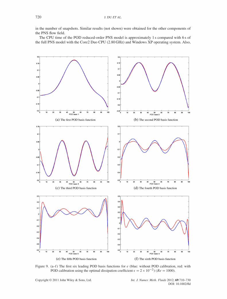
in the number of snapshots. Similar results (not shown) were obtained for the other components ofthe PNS flow field.
The CPU time of the POD reduced-order PNS model is approximately 1 s compared with 6 s ofthe full PNS model with the Core2 Duo CPU (2.80 GHz) and Windows XP operating system. Also,
(a) The first POD basis function (b) The second POD basis function
(c) The third POD basis function (d) The fourth POD basis function
(e) The fifth POD basis function (f) The sixth POD basis function
Figure 9. (a–f) The first six leading POD basis functions for e (blue: without POD calibration, red: withPOD calibration using the optimal dissipation coefficient D 2� 10�2) (Re D 1000).
Copyright © 2011 John Wiley & Sons, Ltd. Int. J. Numer. Meth. Fluids 2012; 69:710–730DOI: 10.1002/fld

REDUCED-ORDER MODELING BASED ON POD OF A PNS EQUATION MODEL 721
(a) (b)
Figure 10. The (a) root mean square error (RMSE) and the (b) correlation coefficient for e between thefull and POD reduced-order PNS models (blue: without POD calibration, red: with POD calibration)
(Re D 1000).
Figure 11. The initial condition for the specific energy e at the inflow boundary A (see Figure 1).
(a) The relation between and the RMSE for e (b) The relation between and the correlation
coefficient for e
Figure 12. The variation of the (a) root mean square error (RMSE) and the (b) correlation coefficient as afunction of different values of the dissipation coefficient (Re D 1000).
Copyright © 2011 John Wiley & Sons, Ltd. Int. J. Numer. Meth. Fluids 2012; 69:710–730DOI: 10.1002/fld

722 J. DU ET AL.
the CPU time spent on the POD basis construction process was only 0.2 s, which is very efficientcompared with the simulation process.
5.2. Numerical results obtained with the H1 norm
Because our model uses a high Reynolds number (e.g. Re D 103), a calibration applied to the PODconstruction process [21–27] is expected to yield better numerical results. In the Sobolev H1 innerproduct norm POD calibration, it is very important to choose an appropriate dissipation coefficient to improve the POD method efficiently. We tested the H1 norm POD calibration for the PNS modelwith Re D 1.0� 103, Re D 0.6� 103, and Re D 1.2� 103.
5.2.1. Re D 1.0 � 103. For the Reynolds number Re D 1.0 � 103, we carried out a series ofnumerical experiments to determine the optimal dissipation coefficient for the specific energy ecorresponding to our test problem.
First, we chose the value of in the interval 10�3 6 6 10 in increments of 10 to test the varia-tion of the RMSE and the COR for the specific energy e between the full PNS model and the PODreduced-order model. The optimal value was found to be D 10�2 (see Figure 7).
A more precise value of for the specific energy e was sought in the vicinity of 10�2 particularly.The RMSE and the COR corresponding to different values of in the interval 2�10�3 6 6 4�10�2are presented in Figure 8, in which we can observe that the smallest RMSE and the largest corre-lation number (0 6 COR 6 1) for the specific energy e between the full PNS model and the PODreduced-order one were both attained for a value of D 2� 10�2.
Figure 9 presents the first six leading POD basis functions with and without H1 norm PODcalibration when the optimal dissipation coefficient D 2� 10�2 was chosen.
The RMSE and the COR of the specific energy e between the full PNS model and the reduced-order PNS model using 100 snapshots with and without the Sobolev H1 norm POD calibration arepresented in Figure 10. We can conclude that the POD method with the Sobolev H1 norm cali-bration and optimal dissipation coefficient improves the long-term stability of the reduced-ordermodel.
Another inflow condition at the inflow boundary A (x D 0, Figure 1) is presented in Figure 11.The variations of the RMSE and the COR for the specific energy e corresponding to different valuesof the dissipation coefficient in the interval 10�3 6 6 10 and 2 � 10�2 6 6 4 � 10�1 arepresented in Figures 12 and 13, respectively. The optimal dissipation coefficient with the smallestRMSE and the largest correlation number turned out to be D 2� 10�2.
(a) The relation between and the RMSE for e (b) The relation between and the correlation coefficient for e
Figure 13. The variation of the (a) root mean square error (RMSE) and the (b) correlation coefficient as afunction of different values of the dissipation coefficient (Re D 1000).
Copyright © 2011 John Wiley & Sons, Ltd. Int. J. Numer. Meth. Fluids 2012; 69:710–730DOI: 10.1002/fld
REDUCED-ORDER MODELING BASED ON POD OF A PNS EQUATION MODEL 723
(a) The first POD basis function (b) The second POD basis function
(c) The third POD basis function (d) The fourth POD basis function
(e) The fifth POD basis function (f) The sixth POD basis function
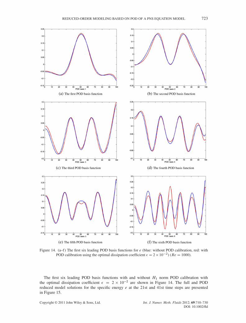
Figure 14. (a–f) The first six leading POD basis functions for e (blue: without POD calibration, red: withPOD calibration using the optimal dissipation coefficient D 2� 10�2) (Re D 1000).
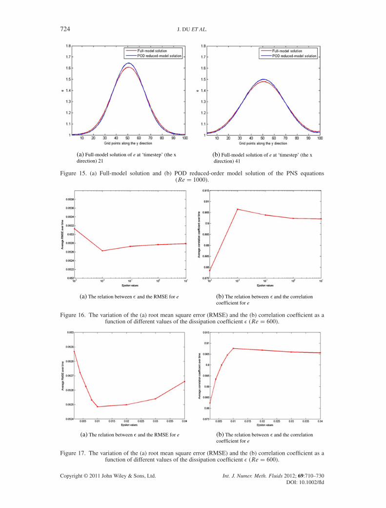
The first six leading POD basis functions with and without H1 norm POD calibration withthe optimal dissipation coefficient D 2 � 10�2 are shown in Figure 14. The full and PODreduced model solutions for the specific energy e at the 21st and 41st time steps are presentedin Figure 15.
Copyright © 2011 John Wiley & Sons, Ltd. Int. J. Numer. Meth. Fluids 2012; 69:710–730DOI: 10.1002/fld
724 J. DU ET AL.
(a) Full-model solution of e at ‘timestep’ (the x direction) 21
(b) Full-model solution of e at ‘timestep’ (the x direction) 41
Figure 15. (a) Full-model solution and (b) POD reduced-order model solution of the PNS equations(Re D 1000).
(a) The relation between and the RMSE for e (b) The relation between and the correlation coefficient for e
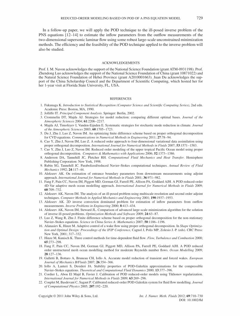
Figure 16. The variation of the (a) root mean square error (RMSE) and the (b) correlation coefficient as afunction of different values of the dissipation coefficient (Re D 600).
(a) The relation between and the RMSE for e (b) The relation between and the correlation coefficient for e
Figure 17. The variation of the (a) root mean square error (RMSE) and the (b) correlation coefficient as afunction of different values of the dissipation coefficient (Re D 600).
Copyright © 2011 John Wiley & Sons, Ltd. Int. J. Numer. Meth. Fluids 2012; 69:710–730DOI: 10.1002/fld

REDUCED-ORDER MODELING BASED ON POD OF A PNS EQUATION MODEL 725
5.2.2. Re D 0.6�103. A similar series of numerical experiments to determine the optimal dissipa-tion coefficient for the specific energy e was carried out for the Reynolds number Re D 0.6�103.Figures 16 and 17 show the variation of the RMSE and the COR for the specific energy e with
respect to different values of in the interval 10�3 6 6 10 and 2 � 10�3 6 6 4 � 10�2,respectively. The optimal value was found to be D 1� 10�2.
(a) The first POD basis function (b) The second POD basis function
(c) The third POD basis function (d) The fourth POD basis function
(e) The fifth POD basis function (f) The sixth POD basis function
Figure 18. (a–f) The first six leading POD basis functions for e (blue: without POD calibration, red: withPOD calibration using the optimal dissipation coefficient D 1� 10�2) (Re D 600).
Copyright © 2011 John Wiley & Sons, Ltd. Int. J. Numer. Meth. Fluids 2012; 69:710–730DOI: 10.1002/fld

726 J. DU ET AL.
(a) Full-model solution of e at ‘timestep’ (the x direction) 21
(b) Full-model solution of e at ‘timestep’ (the x direction) 41
Figure 19. (a) Full-model solution and (b) POD reduced-order model solution of the PNS equations(Re = 600).
(a) The relation between and the RMSE for e (b) The relation between and the correlation coefficient for e
Figure 20. The variation of the (a) root mean square (RMSE) and the (b) correlation coefficient as a functionof different values of the dissipation coefficient (Re D 1200).
(a) The relation between the dissipation coeffi-cient and the RMSE for e
(b) The relation between the dissipation coeffi-cient and the correlation coefficient for e
Figure 21. The variation of the (a) root mean square error (RMSE) and the correlation coefficient as afunction of different values of the dissipation coefficient (Re D 1200).
Copyright © 2011 John Wiley & Sons, Ltd. Int. J. Numer. Meth. Fluids 2012; 69:710–730DOI: 10.1002/fld

REDUCED-ORDER MODELING BASED ON POD OF A PNS EQUATION MODEL 727
Figure 18 presents the first six leading POD basis functions with and without H1 norm PODcalibration using the optimal dissipation coefficient D 1� 10�2.
The full-model solutions compared with the corresponding POD reduced-order solutions for thespecific energy e at the 21st and 41st x-direction nodes are shown in Figure 19.
(a) The first POD basis function (b) The second POD basis function
(c) The third POD basis function (d) The fourth POD basis function
(e) The fifth POD basis function (f) The sixth POD basis function
Figure 22. (a–f) The first six leading POD basis functions for e (blue: without POD calibration, red: withPOD calibration using the optimal dissipation coefficient D 8� 10�2) (Re D 1200).
Copyright © 2011 John Wiley & Sons, Ltd. Int. J. Numer. Meth. Fluids 2012; 69:710–730DOI: 10.1002/fld

728 J. DU ET AL.
5.2.3. Re D 1.2� 103. We carried out the same tests for the optimal dissipation coefficient witha higher Reynolds number of Re D 1.2 � 103. The RMSE and the COR for the specific energy ecorresponding to different values of in the interval 10�3 6 6 10 and 2�10�2 6 6 4�10�1 arepresented in Figures 20 and 21, respectively. The smallest RMSE and the largest correlation numberwere both obtained when D 8� 10�2.
The first six leading POD basis functions with and without H1 norm POD calibration using theoptimal dissipation coefficient D 8� 10�2 are presented in Figure 22.
Figure 23 shows the full-model solutions compared with the corresponding POD reduced-ordersolutions for the specific energy e at the 21st and 41st x-direction nodes.
In conclusion, the optimal dissipation coefficient varied as we increased the Reynolds numberin the PNS equations. The optimal dissipation coefficients for the PNS model with the Reynoldsnumber Re D 0.6� 103, Re D 1� 103, and Re D 1.2� 103 are 1� 10�2, 2� 10�2, and 8� 10�2,respectively, which are all of the order 10�2 and increase in magnitude as the Reynolds numberbecomes higher.
6. CONCLUSIONS AND FUTURE WORK
In this paper, a POD method is applied to derive a reduced-order model for the PNS equations. First,ensembles of snapshots were computed from transient solutions (along the x direction) obtainedwith the space-marching finite difference scheme, and this process can be omitted in actual applica-tions where the ensemble of snapshots can be obtained from physical system trajectories by drawingsamples from experiments and interpolation (or data assimilation). Then, we derived the POD basisfunctions from the ensembles of snapshots and developed the reduced-order model, in which amuch smaller number of the POD basis functions make the reduced-order model optimal in thesense of energy captured. To improve the accuracy and the stability of the reduced-order model inthe presence of increasingly higher Reynolds number, we applied the Sobolev H1 norm calibrationto the POD method. Finally, a number of numerical experiments were carried out to demonstratethe accuracy of the POD reduced-order model compared with the full PNS model. The efficiencyof the H1 norm POD calibration in the presence of high Reynolds number was demonstrated. Anoptimal dissipation coefficient yielding the best RMSE and COR between the full and reduced-order PNS models was estimated for several cases of various Reynolds numbers. We also tested theimpact of the number of snapshots and different inflow conditions on the performance of the PODreduced-order model.
(a) Full-model solution of the specific energy e at ‘timestep’ (the xdirection) 21
(b) Full-model solution of the specific energy e at ‘timestep’ (the xdirection) 41
Figure 23. (a) Full-model solution and (b) POD reduced-order model solution of the PNS equations(Re D 1200).
Copyright © 2011 John Wiley & Sons, Ltd. Int. J. Numer. Meth. Fluids 2012; 69:710–730DOI: 10.1002/fld
REDUCED-ORDER MODELING BASED ON POD OF A PNS EQUATION MODEL 729
In a follow-up paper, we will apply the POD technique to the ill-posed inverse problem of thePNS equations [12–14] to estimate the inflow parameters from the outflow measurements of thetwo-dimensional supersonic laminar flow using some robust large-scale unconstrained minimizationmethods. The efficiency and the feasibility of the POD technique applied to the inverse problem willalso be studied.
ACKNOWLEDGEMENTS
Prof. I. M. Navon acknowledges the support of the National Science Foundation (grant ATM-0931198). Prof.Zhendong Luo acknowledges the support of the National Science Foundation of China (grant 10871022) andthe Natural Science Foundation of Hebei Province (grant A2010001663). Juan Du acknowledges the sup-port of the China Scholarship Council and the Department of Scientific Computing, which hosted her forher 1-year visit at Florida State University, FL, USA.
REFERENCES
1. Fukunaga K. Introduction to Statistical Recognition (Computer Science and Scientific Computing Series), 2nd edn.Academic Press: Boston, MA, 1990.
2. Jolliffe IT. Principal Component Analysis. Springer: Berlin, 2002.3. Crommelin DT, Majda AJ. Strategies for model reduction: comparing different optimal bases. Journal of the
Atmospheric Sciences 2004; 61:2206–2217.4. Majda AJ, Timofeyev I, Vanden-Eijnden E. Systematic strategies for stochastic mode reduction in climate. Journal
of the Atmospheric Sciences 2003; 60:1705–1723.5. Du J, Zhu J, Luo Z, Navon IM. An optimizing finite difference scheme based on proper orthogonal decomposition
for CVD equations. Communications in Numerical Methods in Engineering 2011; 27:78–94.6. Cao Y, Zhu J, Navon IM, Luo Z. A reduced order approach to four-dimensional variational data assimilation using
proper orthogonal decomposition. International Journal for Numerical Methods in Fluids 2007; 53:1571–1583.7. Cao Y, Zhu J, Luo Z, Navon IM. Reduced order modeling of the upper tropical Pacific Ocean model using proper
orthogonal decomposition. Computers & Mathematics with Applications 2006; 52:1373–1386.8. Anderson DA, Tannehill JC, Pletcher RH. Computational Fluid Mechanics and Heat Transfer. Hemisphere
Publishing Corporation: New York, 1998.9. Rubin SG, Tannehill JC. Parabolized/reduced Navier–Stokes computational techniques. Annual Review of Fluid
Mechanics 1992; 24:117–44.10. Alekseev AK. On estimation of entrance boundary parameters from downstream measurements using adjoint
approach. International Journal for Numerical Methods in Fluids 2001; 36:971–982.11. Fang F, Pain CC, Navon IM, Piggott MD, Gorman GJ, Farrell PE, Allison PA, Goddard AJH. A POD reduced-order
4D-Var adaptive mesh ocean modelling approach. International Journal for Numerical Methods in Fluids 2009;60:709–732.
12. Alekseev AK, Navon IM. The analysis of an ill-posed problem using multiscale resolution and second order adjointtechniques. Computer Methods in Applied Mechanics and Engineering 2001; 190:1937–1953.
13. Alekseev AK. 2D inverse convection dominated problem for estimation of inflow parameters from outflowmeasurements. Inverse Problems in Engineering 2000; 8:413–434.
14. Alekseev AK, Navon IM, Steward JL. Comparison of advanced large-scale minimization algorithm for the solutionof inverse ill-posed problems. Optimization Methods and Software 2009; 24:63–87.
15. Luo Z, Wang R, Zhu J. Finite difference scheme based on proper orthogonal decomposition for the non-stationaryNavier–Stokes equations. Science in China Series A: Mathematics 2007; 50:1186–1196.
16. Afanasiev K, Hinze M. Adaptive control of a wake flow using proper orthogonal decomposition. In Shape Optimiza-tion and Optimal Design: Proceedings of the IFIP Conference, Cagnol J, Polis MP, Zolesio J.-P. (eds). CRC Press:New York, 2001; 317–332.
17. Hinze M, Kunisch K. Three control methods for time-dependent fluid flow. Flow, Turbulence and Combustion 2000;65:273–298.
18. Fang F, Pain CC, Navon IM, Gorman GJ, Piggott MD, Allison PA, Farrell PE, Goddard AJH. A POD reducedorder unstructured mesh ocean modelling method for moderate Reynolds number flows. Ocean Modelling 2009;28:127–136.
19. Galletti B, Bottaro A, Bruneau CH, Iollo A. Accurate model reduction of transient and forced wakes. EuropeanJournal of Mechanics B/Fluids 2007; 26:354–366.
20. Iollo A, Lanteri S, Desideri JA. Stability properties of POD-Galerkin approximations for the compressibleNavier–Stokes equations. Theoretical and Computational Fluid Dynamics 2000; 13:377–396.
21. Cordier L, Abou El Majd B, Favier J. Calibration of POD reduced-order models using Tikhonov regularization.International Journal for Numerical Methods in Fluids 2009; 63:269–296.
22. Couplet M, Basdevant C, Sagaut P. Calibrated reduced-order POD-Galerkin system for fluid flow modelling. Journalof Computational Physics 2005; 207:192–220.
Copyright © 2011 John Wiley & Sons, Ltd. Int. J. Numer. Meth. Fluids 2012; 69:710–730DOI: 10.1002/fld

730 J. DU ET AL.
23. Galletti B, Bruneau CH, Zannetti L, Iollo A. Low-order modelling of laminar flow regimes past a confined squarecylinder. Journal of Fluid Mechanics 2004; 503:161–170.
24. Noack BR, Afanasiev K, Morzynski M, Tadmor G, Thiele F. A hierarchy of low-dimensional models for the transientand post-transient cylinder wake. Journal of Fluid Mechanics 2003; 497:335–363.
25. Bourguet R, Braza M, Harran G, Dervieux A. Low-order modeling for unsteady separated compressible flows byPOD-Galerkin approach. IUTAM Symposium on Unsteady Separated Flows and Their Control. Springer: Heidelberg,2009.
26. Sirisup S, Karniadakis GE. A spectral viscosity method for correcting the long-term behavior of POD models.Journal of Computational Physics 2004; 194:92–116.
27. Ullmann S, Lang J. A POD-Galerkin reduced model with updated coefficients for Smagorinsky LES. ECCOMAS-CFD 2010 Fifth European Conference on Computational Fluid Dynamics, Lisbon, Portugal, June 14–17, 2010.
Copyright © 2011 John Wiley & Sons, Ltd. Int. J. Numer. Meth. Fluids 2012; 69:710–730DOI: 10.1002/fld