Recurrent Neural Networks 1: Modelling sequential data · Recurrent Neural Networks 1: Modelling...
23
Recurrent neural networks Modelling sequential data MLP Lecture 9 Recurrent Neural Networks 1: Modelling sequential data 1
Transcript of Recurrent Neural Networks 1: Modelling sequential data · Recurrent Neural Networks 1: Modelling...
Recurrent neural networksModelling sequential data
MLP Lecture 9 Recurrent Neural Networks 1: Modelling sequential data 1
Recurrent Neural Networks 1: Modelling sequential data
Steve Renals
Machine Learning Practical — MLP Lecture 915 November 2017 / 20 November 2017
MLP Lecture 9 Recurrent Neural Networks 1: Modelling sequential data 2
Sequential Data
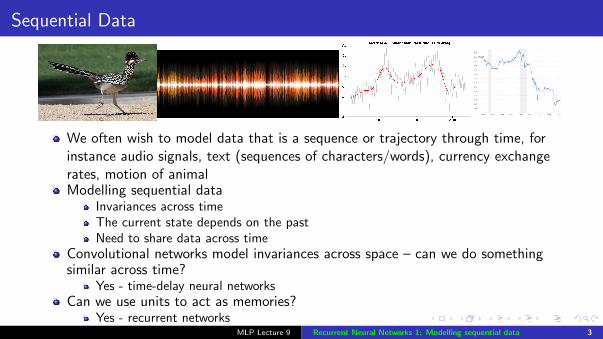
We often wish to model data that is a sequence or trajectory through time, forinstance audio signals, text (sequences of characters/words), currency exchangerates, motion of animalModelling sequential data
Invariances across timeThe current state depends on the pastNeed to share data across time
Convolutional networks model invariances across space – can we do somethingsimilar across time?
Yes - time-delay neural networksCan we use units to act as memories?
Yes - recurrent networksMLP Lecture 9 Recurrent Neural Networks 1: Modelling sequential data 3
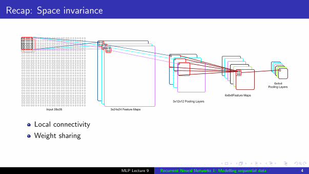
Recap: Space invariance
Input 28x28 3x24x24 Feature Maps
3x12x12 Pooling Layers
6x8x8Feature Maps
6x4x4 Pooling Layers
Local connectivity
Weight sharing
MLP Lecture 9 Recurrent Neural Networks 1: Modelling sequential data 4
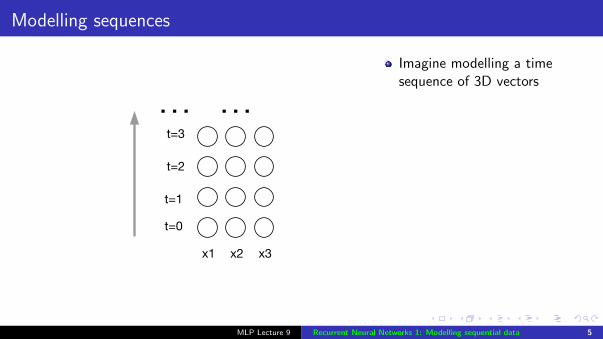
Modelling sequences
t=0
t=1
t=2
t=3
. . . . . .
x1 x2 x3
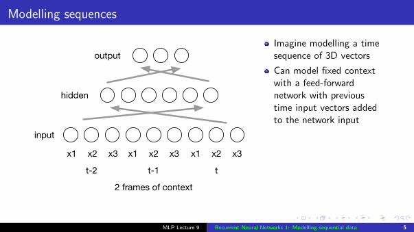
Imagine modelling a timesequence of 3D vectors
Can model fixed contextwith a feed-forwardnetwork with previoustime input vectors addedto the network input
Model using 1-dimensionconvolutions in time -time-delay neuralnetwork (TDNN)
Network takes intoaccount a finite context
MLP Lecture 9 Recurrent Neural Networks 1: Modelling sequential data 5
Modelling sequences
t-2
x1 x2 x3 x1 x2 x3
t-1
x1 x2 x3
t
output
hidden
input
2 frames of context
Imagine modelling a timesequence of 3D vectors
Can model fixed contextwith a feed-forwardnetwork with previoustime input vectors addedto the network input
Model using 1-dimensionconvolutions in time -time-delay neuralnetwork (TDNN)
Network takes intoaccount a finite context
MLP Lecture 9 Recurrent Neural Networks 1: Modelling sequential data 5
Modelling sequences
t-2
x1
x2
x3
t-1 t
output
1D convlayer
inputt-3
fully-connectedlayer
. . .
. . .
t-T
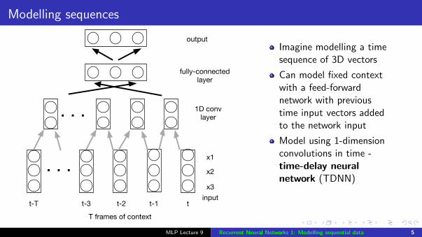
T frames of context
Imagine modelling a timesequence of 3D vectors
Can model fixed contextwith a feed-forwardnetwork with previoustime input vectors addedto the network input
Model using 1-dimensionconvolutions in time -time-delay neuralnetwork (TDNN)
Network takes intoaccount a finite context
MLP Lecture 9 Recurrent Neural Networks 1: Modelling sequential data 5
Modelling sequences
t-2
x1
x2
x3
t-1 t
output
1D convlayer
inputt-3
fully-connectedlayer
. . .
. . .
t-T
T frames of context
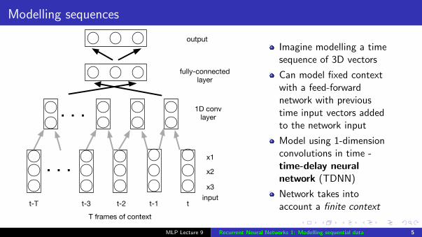
Imagine modelling a timesequence of 3D vectors
Can model fixed contextwith a feed-forwardnetwork with previoustime input vectors addedto the network input
Model using 1-dimensionconvolutions in time -time-delay neuralnetwork (TDNN)
Network takes intoaccount a finite context
MLP Lecture 9 Recurrent Neural Networks 1: Modelling sequential data 5
TDNNs in action
tackle late reverberations, DNNs should be able to model tem-poral relationships across wide acoustic contexts.
TDNNs [5], which are feed-forward neural networks, withthe ability to model long-term temporal relationships, were usedhere. We used the sub-sampling technique proposed in [6] toachieve an acceptable training time.
In Section 3 we describe the time delay neural network ar-chitecture in greater detail.
3. Neural network architectureIn a TDNN architecture the initial transforms are learnt on nar-row contexts and the deeper layers process the hidden activa-tions from increasingly wider contexts. Hence the higher layershave the ability to learn longer temporal relationships. Howeverthe training time of a TDNN is substantially larger than that ofa DNN, when modeling long temporal contexts, despite the useof speed-up techniques such as [19].
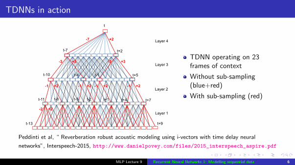
In [6] a sub-sampling technique was proposed to reduce thenumber of hidden activations computed in the TDNN, while en-suring that the information from all time steps in the input con-text was used. Figure 1 shows time steps at which activationsare computed, at each layer, and the dependencies between ac-tivations across layers, both in a conventional TDNN (blue+rededges) and a sub-sampled TDNN (red edges), in order to com-pute the network output at time t. The use of sub-samplingspeeds up the training by ⇠ 5x in the baseline TDNN architec-ture shown in Figure 1.
t-4
-1 +2
t
t-7 t+2
t-10 t-1 t+5
t-11 t+7
t-13 t+9
-7 +2
-1 +2
-2 +2
-1 +2 -1 +2
-3 +3 -3 +3
t+1 t+4 t-2 t-5 t-8
Layer 4
Layer 3
Layer 2
Layer 1
Figure 1: Computation in TDNN with sub-sampling (red) andwithout sub-sampling (blue+red)
The hyper-parameters which define the sub-sampled TDNNnetwork structure are the set of frame offsets that we requireas an input to each layer. In the case pictured, these are{�2,�1, 0, 1, 2}, {�1, 2}, {�3, 3} and {�7, 2}. In a conven-tional TDNN, these input frame offsets would always be con-tiguous. However, in our work we sub-sample these; in ournormal configuration, the frame splicing at the hidden layerssplices together just two frames, separated by a delay that in-creases as we go to higher layers of the network [6].
In this paper we were able to operate on input contexts of upto 280 ms without detriment in performance, using the TDNN.Thus the TDNN has the capability to tackle corruptions due tolate reverberations.
Our TDNN uses the p-norm non-linearity [20]. We use agroup size of of 10, and the 2-norm.
3.1. Input Features
Mel-frequency cepstral coefficients (MFCCs) [21], withoutcepstral truncation, were used as input to the neural network.40 MFCCs were computed at each time index. MFCCs over awide asymmetric temporal context were provided to the neuralnetwork. Different contexts were explored in this paper. 100dimensional iVectors were also provided as an input to the net-work, every time frame. Section 4 describes the iVector extrac-tion process during training and decoding in greater detail.
3.2. Training recipe
The paper follows the training recipe detailed in [20]. It usesgreedy layer-wise supervised training, preconditioned stochas-tic gradient descent (SGD) updates, an exponentially decreas-ing learning rate schedule and mixing-up. Parallel training ofthe DNNs using up to 18 GPUs was done using the model aver-aging technique in [13].
3.2.1. Modified sMBR sequence training
Sequence training was done on the DNN, based on a state-levelvariant of the Minimum Phone Error (MPE) criterion, calledsMBR [22] . The training recipe mostly follows [23], althoughit has been modified for the parallel-training method. Trainingis run in parallel using 12 GPUs, while periodically averagingthe parameters, just as in the cross-entropy training phase.
Our previous sMBR-based training recipe degraded resultson the ASpIRE setup, so we introduced a modification to therecipe which we have since found to be useful more generally,in other LVCSR tasks.
In the sMBR objective function, as for MPE, insertion er-rors are not penalized. This can lead to larger number of inser-tion errors when decoding with sMBR trained acoustic models.Correcting this asymmetry in the sMBR objective function, bypenalizing insertions, was shown to improve the WER perfor-mance of sMBR models by 10% relative. In standard sMBRtraining [22, 24], the frame error is always set to zero if thereference is silence, which means that insertions into silenceregions are not penalized. In other words, frames where thereference alignment is silence are treated specially. (Note thatin our implementation several phones, including silence, vo-calized noise and non-spoken noise, are treated as silence forthese purposes.) In our modified sMBR training method, wetreat silence as any other phone, except that all pdfs of silencephones are collapsed into a single class for the frame-error com-putation. This means that replacing one silence phone with an-other silence phone is not penalized (e.g. replacing silence withvocalized-noise is not penalized), but insertion of a non-silencephone into a silence region is penalized. This is closer to theWER metric that we actually care about, since WER is gener-ally computed after filtering out noises, but does penalize in-sertions. We call our modified criterion the “one-silence-class”modification of sMBR.
4. iVector ExtractionIn this section we describe the iVector estimation processadopted during training and decoding. We discuss issues in es-timating iVectors from noisy unsegmented speech recordings,and in using these noisy estimates of iVectors as input to neuralnetworks.
On each frame we append a 100-dimensional iVector [25]to the 40-dimensional MFCC input. The MFCC input is not
TDNN operating on 23frames of context
Without sub-sampling(blue+red)
With sub-sampling (red)
Peddinti et al, “ Reverberation robust acoustic modeling using i-vectors with time delay neural
networks”, Interspeech-2015, http://www.danielpovey.com/files/2015_interspeech_aspire.pdf
MLP Lecture 9 Recurrent Neural Networks 1: Modelling sequential data 6
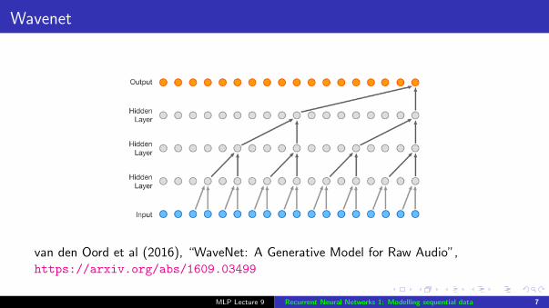
Wavenet
van den Oord et al (2016), “WaveNet: A Generative Model for Raw Audio”,https://arxiv.org/abs/1609.03499
MLP Lecture 9 Recurrent Neural Networks 1: Modelling sequential data 7
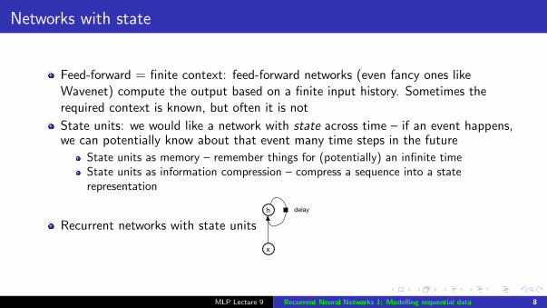
Networks with state
Feed-forward = finite context: feed-forward networks (even fancy ones likeWavenet) compute the output based on a finite input history. Sometimes therequired context is known, but often it is not
State units: we would like a network with state across time – if an event happens,we can potentially know about that event many time steps in the future
State units as memory – remember things for (potentially) an infinite timeState units as information compression – compress a sequence into a staterepresentation
Recurrent networks with state units
delayh
x
MLP Lecture 9 Recurrent Neural Networks 1: Modelling sequential data 8
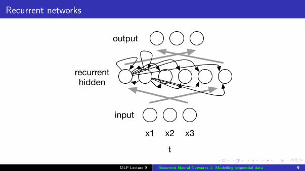
Recurrent networks
x1 x2 x3
t
output
recurrenthidden
input
MLP Lecture 9 Recurrent Neural Networks 1: Modelling sequential data 9
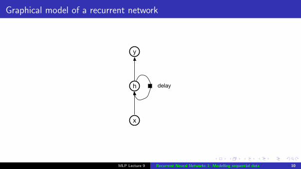
Graphical model of a recurrent network
delayh
x
y
MLP Lecture 9 Recurrent Neural Networks 1: Modelling sequential data 10
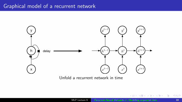
Graphical model of a recurrent network
delayh
x
y
ht�1
xt�1
yt�1
ht ht+1
xt+1xt
yt yt+1
Unfold a recurrent network in time
MLP Lecture 9 Recurrent Neural Networks 1: Modelling sequential data 10
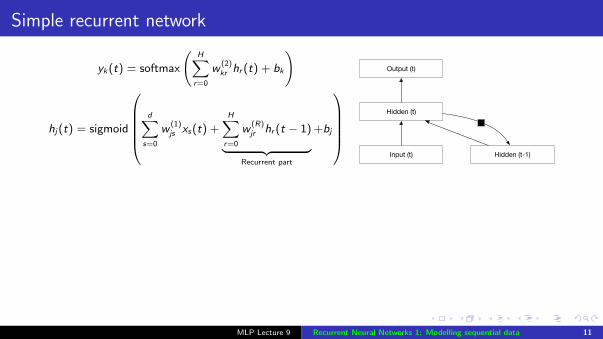
Simple recurrent network
yk(t) = softmax
(H∑
r=0
w(2)kr hr (t) + bk
)
hj(t) = sigmoid
d∑
s=0
w(1)js xs(t) +
H∑r=0
w(R)jr hr (t − 1)︸ ︷︷ ︸
Recurrent part
+bj
Output (t)
Hidden (t)
Input (t) Hidden (t-1)
MLP Lecture 9 Recurrent Neural Networks 1: Modelling sequential data 11
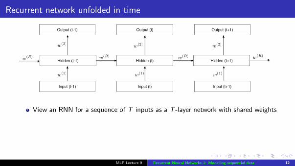
Recurrent network unfolded in time
Hidden (t)
Output (t)
Input (t)
Hidden (t-1)
w(1)
w(2)
w(R)
Hidden (t+1)
Input (t-1)
Output (t-1)
Input (t+1)
Output (t+1)
w(2)w(2)
w(1)w(1)
w(R)w(R) w(R)
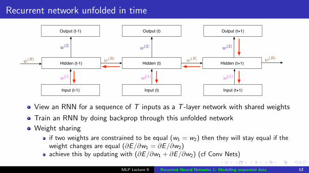
View an RNN for a sequence of T inputs as a T -layer network with shared weights
Train an RNN by doing backprop through this unfolded networkWeight sharing
if two weights are constrained to be equal (w1 = w2) then they will stay equal if theweight changes are equal (∂E/∂w1 = ∂E/∂w2)achieve this by updating with (∂E/∂w1 + ∂E/∂w2) (cf Conv Nets)
MLP Lecture 9 Recurrent Neural Networks 1: Modelling sequential data 12
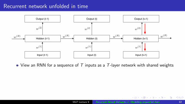
Recurrent network unfolded in time
Hidden (t)
Output (t)
Input (t)
Hidden (t-1)
w(1)
w(2)
w(R)
Hidden (t+1)
Input (t-1)
Output (t-1)
Input (t+1)
Output (t+1)
w(2)w(2)
w(1)w(1)
w(R)w(R) w(R)
View an RNN for a sequence of T inputs as a T -layer network with shared weights
Train an RNN by doing backprop through this unfolded network
Weight sharing
if two weights are constrained to be equal (w1 = w2) then they will stay equal if theweight changes are equal (∂E/∂w1 = ∂E/∂w2)achieve this by updating with (∂E/∂w1 + ∂E/∂w2) (cf Conv Nets)
MLP Lecture 9 Recurrent Neural Networks 1: Modelling sequential data 12
Bidirectional RNN
FHid (t)
Output (t)
Input (t)
FHid (t-1) FHid (t+1)
Input (t-1)
Output (t-1)
Input (t+1)
Output (t+1)
RHid (t)RHid (t-1) RHid (t+1)
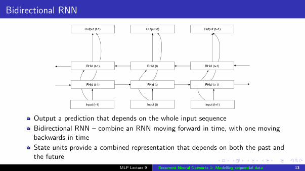
Output a prediction that depends on the whole input sequence
Bidirectional RNN – combine an RNN moving forward in time, with one movingbackwards in time
State units provide a combined representation that depends on both the past andthe future
MLP Lecture 9 Recurrent Neural Networks 1: Modelling sequential data 13
Back-propagation through time (BPTT)
We can train a network by unfolding and back-propagating through time,summing the derivatives for each weight as we go through the sequence
More efficiently, run as a recurrent network
cache the unit outputs at each timestepcache the output errors at each timestepthen backprop from the final timestep to zero, computing the derivatives at each stepcompute the weight updates by summing the derivatives across time
Expensive – backprop for a 1,000 item sequence equivalent to a 1,000-layerfeed-forward network
Truncated BPTT – backprop through just a few time steps (e.g. 20)
MLP Lecture 9 Recurrent Neural Networks 1: Modelling sequential data 14
Example 1: speech recognition with recurrent networks
time (ms)
freq (
Hz)
0 200 400 600 800 1000 1200 14000
2000
4000
6000
8000
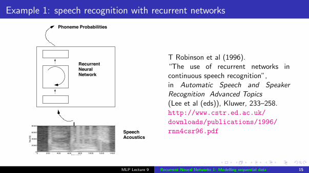
RecurrentNeuralNetwork
SpeechAcoustics
Phoneme Probabilities
T Robinson et al (1996).“The use of recurrent networks incontinuous speech recognition”,in Automatic Speech and SpeakerRecognition Advanced Topics(Lee et al (eds)), Kluwer, 233–258.http://www.cstr.ed.ac.uk/
downloads/publications/1996/
rnn4csr96.pdf
MLP Lecture 9 Recurrent Neural Networks 1: Modelling sequential data 15
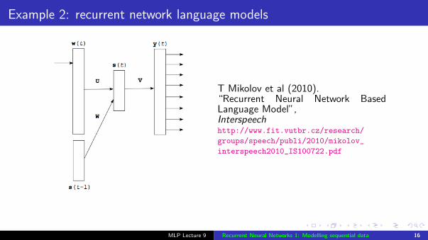
Example 2: recurrent network language models
T Mikolov et al (2010).“Recurrent Neural Network BasedLanguage Model”,Interspeechhttp://www.fit.vutbr.cz/research/
groups/speech/publi/2010/mikolov_
interspeech2010_IS100722.pdf
MLP Lecture 9 Recurrent Neural Networks 1: Modelling sequential data 16
Summary
Model sequences using finite context using feed-forward networks withconvolutions in time (TDNNs, Wavenet)
Model sequences using infinite context using recurrent neural networks (RNNs)
Unfolding an RNN gives a deep feed-forward network with shared weights
Train using back-propagation through time
Back-propagation through time
(Historical) examples on speech recognition and language modelling
Reading: Goodfellow et al, chapter 10 (sections 10.1, 10.2, 10.3)http://www.deeplearningbook.org/contents/rnn.html
Next lecture: LSTM, sequence-sequence models
MLP Lecture 9 Recurrent Neural Networks 1: Modelling sequential data 17