RecentAdvances&in&Numerical&Techniques&for& … seminars... · HFSS (FEM), Comsol (FEM), Many...

Recent Advances in Numerical Techniques for Simula8on of Transient Electromagne8c Wave Interac8ons Hakan Bağcı Electrical Engineering Division of Computer, Electrical, and Mathema8cal Sciences and Engineering King Abdullah University of Science and Technology (KAUST) November 3, 2013 KAUST, Thuwal 23955-‐6900, Saudi Arabia

•  Computational Electromagnetics (CEM) §  Challenges and Applications §  Frequency Domain vs. Time Domain §  Differential Equation vs. Integral Equation Solvers §  CEM Research Group at KAUST

•  Two Recently Developed Time-Domain Solvers Ø  Time Domain Discontinuous Galerkin Method with Exact Boundary Conditions

§  Introduction §  Formulation §  Numerical Results §  Conclusions and Future/Ongoing Work

Ø  Time Domain Volume Integral Equation Solver for High Contrast Scatterers §  Introduction §  Formulation §  Numerical Results §  Conclusions and Future/Ongoing Work

Outline

•  Computational Electromagnetics (CEM) §  Challenges and Applications §  Frequency Domain vs. Time Domain §  Differential Equation vs. Integral Equation Solvers §  CEM Research Group at KAUST

•  What is a “computer simula8on” ?

§  It is an a[empt to model a real-‐life or hypothe8cal problem on a computer so that its solu8on can be es8mated

•  Why do engineers need or prefer computer simula8ons ?

§  Expensive and/or impossible experiments §  Repe88ve processes, typical in design

frameworks §  Expensive human labor, cheap compu8ng

power

•  Fields of electromagne8cs/op8cs/photonics are no different. Simula8on tools are needed.

§  CEM is the solu8on

Simula8on

Applied Mathematics

Engineering

Computer Hardware/Software Models,

approximations, error analysis Computational resources, new and

specially designed architectures, parallelization strategies, programming languages

Simulation Tools for Solving Maxwell Equations

Novel and robust formulations, fast

algorithms

Applications in electromagnetics/optics/

photonics

Multi-physics modeling and simulation frameworks: Coupled problems of structural, thermal,

and electromagnetic applications

Computa8onal Electromagne8cs (CEM)

•  Two types of Methods: §  Differen8al Equa8on Based Solvers §  Integral Equa8on Based Solvers

•  Two Domains: §  Frequency Domain Solvers §  Time Domain Solvers

CEM

j te ωTime-dependence:

Time-derivative: Time-integration: Convolution Multiplication Inverse Fourier Transform to switch to time domain

jt

ω∂ →∂

•  Positives §  Intuitively easier to understand §  Easier to implement in general §  Lower computational cost §  Dispersion is easier to model

•  Negatives §  Strong nonlinearities cannot be modeled §  Only single frequency results, no

broadband data §  Many simulations to obtain broadband

results §  Needs inverse Fourier transform as post-

processors

1

t

dtjω

→∫→

Example Commercial Tools: HFSS (FEM), Comsol (FEM), FISC (MOM), WIPL-D (MOM)

Frequency Domain Simulators

Time-dependence: Arbitrary (band limited)

Fourier Transform to switch to frequency domain

•  Positives §  Strong nonlinearities can be modeled §  Provides broadband data with a single

simulation §  Transient response is easy to get §  Provides immediately the physics, no post-

processing •  Negatives

§  More difficult to implement §  Instabilities §  Methods to handle resonance §  Modeling dispersion requires computation

of (costly) temporal convolutions §  Higher computational cost

Example Commercial Tools: Many available (FDTD), No well-known commercial tools (TD-FEM, MOT-TDIE)

Time Domain Simulators

( , )( , )

( , )( , ) ( , )

( , )( , )

( , ) 0

ttttt tt

tt

t

µ

ε

ρε

∂∇× = −∂

∂∇× = +∂

∇ ⋅ =

∇⋅ =

H rE r

E rH r J r

rE r

H r

Time-dependent:

Time-harmonic: jt

ω∂ →∂

•  Discretize differential form of Maxwell equations •  Approximate derivatives using neighboring

elements (in time and space) •  Positives

§  Straightforward to implement •  Extension to inhomogeneous media is trivial

•  Negatives §  Numerical dispersion §  Truncation of the (open) computation domain §  Discretization of the computation domain §  Typically time step size is constrained by the

spatial discretization §  Inaccurate geometry representation (FDTD)

Example Commercial Tools: HFSS (FEM), Comsol (FEM), Many available (FDTD)

Differen8al Equa8on Based Simulators

( )e ,tJ r

S

V( )e ,tM r

0 0,ε µ

0 0,ε µ

( ),G R t t′−

•  Replace scatterers with equivalent surface and volume currents

•  Find fields due to these currents using Green function

•  Apply boundary conditions to solve for unknowns •  Positives

§  No phase dispersion §  No grid truncation (exact radiation condition) §  Time step size is not necessarily constrained

by spatial discretization §  Only the surface (or volume) of the object is

discretized §  Accurate representation of the geometry

•  Negatives §  More difficult to implement §  Higher computational costs §  Instabilities

incE

( ) ( )inc scatan tan

, ,t tt t∂ = ∂E r E r S∈rBoundary Equation:

Time-harmonic: jt

ω∂ →∂

Example Commercial Tools: FISC (MOM), WPIL-D (MOM), Not available in time domain

Integral Equa8on Based Simulators

•  Applications in electromagnetics/optics/photonics:

§  Radiation, radar, sensing, detection, imaging §  EMC/EMI analysis §  Plasmonics §  THz wave propagation

•  As a part of multi-physics modeling and simulation frameworks (coupled problems of structural, thermal, and electromagnetic applications)

§  Composite antenna design §  Chip design and packaging §  Vehicle (space craft, UAVs, airplanes, cars)

design


•  Some of the challenges in application of CEM tools in real life scenarios

•  Large computation domains (large number of unknowns)

•  Multi-scale geometric features (large number of unknowns, poor conditioning, slow convergence rates)

•  One mesh for multi-physics simulation (multi-scale elements with high aspect ratios, large number of unknowns, poor conditioning)

•  Difficult to model highly oscillatory physical resonances in electrically large models

•  Presence of spurious modes/resonances on complex structures

•  Uncertainties in model descriptions including geometry and excitation parameters, material properties, constitutive relations

•  Loss of accuracy due to increasing complexity


CEM research group at KAUST develops novel 8me domain solvers for characterizing electromagne8c wave interac8ons on electrically large and mul8-‐scale structures and applies them in real-‐life problems of electromagne8cs/op8cs/photonics. More specifically:

•  Explicit and non-‐uniform, yet stable, 8me marching techniques for efficiently solving TDIEs (to address the increase in computa8on 8me due to matrix inversion and large number of unknowns)

•  Mixed space and 8me discre8za8on schemes for TDIEs (for increased accuracy)

•  Exact boundary condi8ons in the form of TDIEs for termina8ng differen8al equa8on solvers (for increased accuracy)

•  Blocked FFT-‐based schemes for accelera8ng the computa8on of space-‐8me convolu8ons in TDIEs (to address the increase in computa8on 8me due to large number of unknowns)

•  Calderòn-‐ and Wavelet-‐based precondi8oners for TDIEs (to address the ill-‐condi8oning due to mul8-‐scale discre8za8ons and low-‐frequency excita8on)

•  Hybridiza8on schemes between different-‐scale solvers in 8me domain [circuit, transmission line, and TDIE solvers] (to address the ill-‐condi8oning due to mul8-‐scale discre8za8ons)

CEM Research Group at KAUST – Research

•  Applica8on of the resul8ng novel methods in §  Inverse sca[ering problems with sparsity constraints

§  Design of plasmonic devices with applica8ons in slow light and metamaterials

§  Uncertainty Quan8fica8on (UQ) frameworks for EMC/EMI characteriza8on on complex electrically large plakorms

§  Sta8s8cal characteriza8on of wave propaga8on in harsh environments

CEM Research Group at KAUST – Research

Work Force PhD Students §  Muhammad Amin

§  Abdulla Desmal §  Ismail Uysal

§  Sadeed Sayed §  Noha Alharthi §  Ali Imran Sandhu

§  Ozum Asirim

Post-‐Doctoral Researchers

§  Kostyantyn Sirenko, PhD §  Arda Ulku, PhD §  Yifei Shi, PhD

§  Mohamed Farhat, PhD

Alumni

§  Mohamed Salem, PhD (Mar. 2013) §  Ahmed Al-‐Jarro, PhD (Nov. 2012) §  Meilin Liu, PhD (Jan. 2012)

§  Umair Khalid (MS degree, Dec. 2010) §  Muhammad Furqan (Feb. 2012)

§  Abdul Haseeb Muhammed (Apr. 2011)

Computa/onal Resources

Shaheen

§  IBM’s 16-‐Rack Blue Gene/P, ~65k compu8ng cores, 222 teraflops/sec

§  Expandable to petascale compu8ng

§  Supported by IBM and KAUST Supercompu8ng Laboratory (KSL)

Noor

§  Beowulf class heterogeneous cluster

§  Intel Xeon X5570, IBM Power6, ~1000 cores

§  Supported by KAUST Research Compu8ng

CEML: h[p://maxwell.kaust.edu.sa

KAUST Supercompu8ng Laboratory: h[p://www.hpc.kaust.edu.sa

CEM Research Group at KAUST – People and Facili8es

•  Time Domain Discontinuous Galerkin Method with Exact Boundary Conditions §  Introduction §  Formulation §  Numerical Results §  Conclusions and Future/Ongoing Work

§  With: Ozum Asirim, Ping Li, Konstyantyn Sirenko, and Yifei Shi

Introduc8on

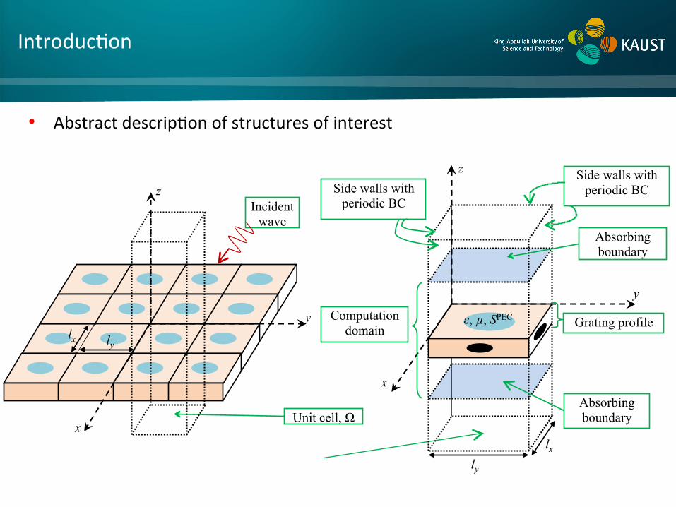
Unit cell, Ω

ly lx

y

z

x

Incident wave

Absorbing boundary

Absorbing boundary

ly lx

y

Computation domain

ε, µ, SPEC

Side walls with periodic BC

Grating profile

x

z Side walls with periodic BC

•  Abstract descrip8on of structures of interest

•  Time Domain Discon8nuous Galerkin Finite Element Methods (TD-‐DG-‐FEM) are an alterna8ve to finite difference 8me domain (FDTD) and classical FEM schemes Advantages §  Informa8on exchange between elements using numerical flux §  All spa8al opera8ons are localized §  Complex/arbitrarily shaped geometries §  Non-‐conformal discre8za8on §  Adap8ve spa8al meshing is easier to implement §  Higher order expansions are easy to implement §  (Block) diagonal mass matrix

Ø Compact solvers when combined with explicit 8me integra8on schemes §  Easier to parallelize Disadvantages §  Increased number of unknowns

Ø  Disadvantage diminishes as expansion order increases

Introduc8on

Introduc8on

•  TD-‐DG-‐FEM is naturally a (spa8ally) high-‐order accuracy method •  Accuracy is ouen limited by

§  Computa8on domain trunca8on (PML or approximate absorbing boundary condi8ons) in unbounded space problems Ø Increase thickness of PML at the cost of efficiency

Proposed Solu/ons •  Exact absorbing boundary condi8ons with FFT accelera8on

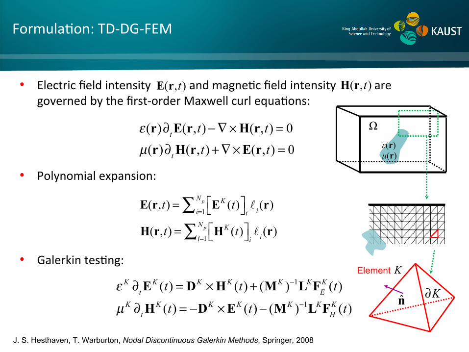
•  Electric field intensity and magne8c field intensity are governed by the first-‐order Maxwell curl equa8ons:

•  Polynomial expansion:

•  Galerkin tes8ng:

ε(r)∂t E(r,t)−∇× H(r,t) = 0 µ(r)∂t H(r,t)+∇×E(r,t) = 0

ε K ∂t EK (t) = DK × HK (t)+ (MK )−1LKFE

K (t)

µK ∂t HK (t) = −DK ×EK (t)− (MK )−1LKFH

K (t)

J. S. Hesthaven, T. Warburton, Nodal Discontinuous Galerkin Methods, Springer, 2008

E(r,t) = EK (t)⎡⎣ ⎤⎦i i (r)

i=1

N p∑H(r,t) = HK (t)⎡⎣ ⎤⎦i

i (r)i=1

N p∑

Formula8on: TD-‐DG-‐FEM

E(r,t) H(r,t)

Ω ε(r) µ(r)

Element

n ∂K

K


K (t)


K (t)



where

•  Field samples to be computed:

•  Differen8a8on matrices:

• Mass matrices:

•  Face/liu matrices:

[Ev

K (t)]i = Ev ,iK (t), [Hv

K (t)]i = Hv ,iK (t), v ∈ x, y,z{ }

[Dv

K ]ij = ∂v j (ri ), v ∈ x, y,z{ }

[MK ]ij = i (r) j (r)dr

K∫

[LK ]ij = i (r) j (r)dr

∂K∫ , j ∈{ j :rj ∈∂K}

•  Up-‐winding numerical flux for Maxwell equa8ons:

•  Here, , ,


K (t)


K (t)



– +

’s neighbor EK− HK−

EK+ HK+ n

FEK (t) = n× (Z +ΔHK − n× ΔEK )

Z + + Z −

FHK (t) = n× (Y +ΔEK + n× ΔHK )

Y + +Y −

1/21 / ( / )Z Y± ± ± ±= = µ ε ΔEK = EK+ (t)−EK− (t) ΔHK = HK+ (t)− HK− (t)

Element K

K

•  Numerical flux

§  Informa8on exchange between elements

§  Stability of the whole numerical scheme

§  Impose PEC boundary condi8ons

§  Impose periodic boundary condi8ons: “neighboring” elements are on the opposite sides of computa8on domain, but connected via numerical flux

§  Impose exact absorbing boundary condi8ons (EACs)—described next…

Z+ = Z − , Y + = Y −


ΔHK = 0, ΔEK = −2EK− (t)

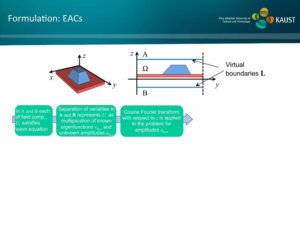
∂t2U = ΔU

U ∈ Ex , Ey , Ez , Hx , H y , Hz{ }

In A and B each of field comp., U, satisfies wave equation

y

z

x

z

y

Ω

A

B

Virtual boundaries L

Formula8on: EACs


U (g,t) = um,n(z,t)vm,n(x, y)

m,n=−∞

∞

∑

∂t2um,n(z,t) = ∂z

2um,n(z,t)−νm,n2 um,n(z,t)

um,n(z,0) = ∂t um,n(z,t)t=0

= 0

y

z

x

z

y

Ω

A

B


Formula8on: EACs

Separation of variables in A and B represents U as multiplication of known eigenfunctions νm,n and

unknown amplitudes um,n


y

z

x

z

y

Ω

A

B


Formula8on: EACs

Cosine Fourier transform with respect to z is applied

to the problem for amplitudes um,n




y

z

x

z

y

Ω

A

B


Formula8on: EACs

Solution of the resulting

generalized Cauchy problem






∂t um,n(L,t) ± ∂z um,n(L,t) =

= −λm,n

J1([t − τ]λm,n )t − τ

um,n(L,τ)dτ0

t

∫

y

z

x

z

y

Ω

A

B


Formula8on: EACs

Inverse Fourier transform is

applied to the solution








EM field comp., U, are reconstructed back from the amplitudes um,n

∂tU (L,t) = ±∂zU (L,t)−

J1([t − τ]λm,n )t − τ

U (L,τ)vm,n*

L∫ dS⎡

⎣⎢⎢

⎤

⎦⎥⎥

dτ0

t

∫⎧⎨⎪

⎩⎪

⎫⎬⎪

⎭⎪λm,nvm,n

m,n=−∞

∞

∑

•  Relates the boundary values with their normal deriva8ve on the virtual boundaries L, and thus could be used as a boundary condi8on

y

z

x

z

y

Ω

A

B


Formula8on: EACs

Inverse Fourier transform is

applied to the solution







•  Convenient for TD-‐DG-‐FEM framework

•  EACs should be discre8zed with the same level of accuracy as TD-‐DG-‐FEM both in space and 8me

•  The summa8ons over m and n are truncated to a finite number of terms, Mh and Nh

•  Field component, U, and eigenfunc8ons, νm,n , are sampled at TD-‐DG-‐FEM’s nodal

points on the virtual boundaries, L

•  Proper (high-‐order) numerical quadrature rules are used for space and 8me integra8ons

Formula8on: EACs

∂tU (L,t) = ±∂zU (L,t)−

J1([t − τ]λm,n )t − τ

U (L,τ)vm,n*

L∫ dS⎡

⎣⎢⎢

⎤

⎦⎥⎥

dτ0

t

∫⎧⎨⎪

⎩⎪

⎫⎬⎪

⎭⎪λm,nvm,n

m,n=−∞

∞

∑

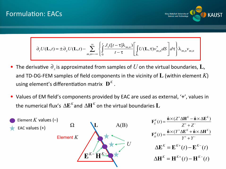
•  The deriva8ve is approximated from samples of U on the virtual boundaries, L, and TD-‐DG-‐FEM samples of field components in the vicinity of L (within element K) using element’s differen8a8on matrix .

•  Values of EM field’s components provided by EAC are used as external, ‘+’, values in the numerical flux’s and on the virtual boundaries L

Element

Ω L A(B)

U

Element values (–)

EAC values (+)

z∂

∂tU (L,t) = ±∂zU (L,t)−

J1([t − τ]λm,n )t − τ

U (L,τ)vm,n*

L∫ dS⎡

⎣⎢⎢

⎤

⎦⎥⎥

dτ0

t

∫⎧⎨⎪

⎩⎪

⎫⎬⎪

⎭⎪λm,nvm,n

m,n=−∞

∞

∑

Formula8on: EACs

EK− HK−

K

K

ΔEK ΔHK

DK

FEK (t) = n× (Z +ΔHK − n× ΔEK )

Z + + Z −

FHK (t) = n× (Y +ΔEK + n× ΔHK )

Y + +Y −

ΔEK = EK+ (t)−EK− (t)

ΔHK = HK+ (t)− HK− (t)

1

1

( ) ( ) ( ) ( )

( ) ( ) ( ) ( )

K K K K K K Kt E

K K K K K K Kt H

t t t

t t t

−

−

∂ = × +

∂ = − × −

E D H M L F

H D E M L F

εµ

1 ,, , ,0

( ) ( )[( ) ]

( )h h

h h

K K Kt z

M N t m nK k k km n m n m nk

m M n N

t tJ t t

t dtt t

′ ′ ′′

=− =−

∂ = ±′−

′ ′−′−∑ ∑ ∑∫

U D U

ν w U νλ

λ

• Maxwell equa8ons and EAC are integrated in 8me simultaneously

Maxwell equations

EAC

Formula8on: System of Equa8ons

O(N 2Nt2 )

Blocked FFTs O(N 2Nt log2 Nt )•  Computa8onal cost:

•  Time Integra8on: Fourth order explicit Runge-‐Ku[a method

exact, no addi8onal numerical error

Numerical Results: Accuracy of EACs

•  Dura8on of simula8on is 7.5

•  Excita8on signal

x

z

y

lx

lz

a a

b

a = 0.42, b = 0.28 lx = lz = 0.5, h= 0.5

Ez

inc (x,1.5, z,t) = 2e−(t−1.5)2 0.13 cos(15[t −1.5])µ0,0 (x, z)

t = 4 t = 5.8

Numerical Results: Mushroom Gra8ngs

•  Height of the structure is 4.1 µm; diameter of PEC inclusions is 0.4 µm •  80150 mesh elements in the computa8on domain. 4 809 000 unknowns •  Excita8on: •  Wavelength at the center frequency is 483 nm

The image cannot be displayed. Your computer may not have enough memory to open the image, or the image may have been corrupted. Restart your computer, and then open the file again. If the red x still appears, you may have to delete the image and then insert it again.

The image cannot be displayed. Your computer may not have enough memory to open the image, or the image may have been corrupted. Restart your computer, and then open the file again. If the red x still appears, you may have to delete the image and then insert it again.

Numerical Results: Mushroom Gra8ngs

•  Highlights: •  Discre8za8on and coupling of EAC equa8ons into TD-‐DG-‐FEM discre8zing

Maxwell equa8on are described •  Numerical results demonstrate the accuracy of EAC discre8za8on •  The accuracy of EAC discre8za8on grows with the order of DG-‐FEM. Thus,

trunca8on of computa8on domain no longer limits the overall accuracy of numerical solu8on

•  Ongoing Work: •  Efficient trunca8on methods for concave geometries •  Incorpora8on of material nonlinearity

Conclusions and Future/Ongoing Work

•  Time Domain Integral Equation Solver for High Contrast Scatterers §  Introduction §  Formulation §  Numerical Results §  Conclusions and Future/Ongoing Work

§  With: Sadeed Bin Sayed and Huseyin Arda Ulku

•  Time Domain Volume Integral Equa8on (TDVIE) Solvers are an alterna8ve to finite difference 8me domain (FDTD) and classical FEM schemes

•  TDVIEs are classically solved using Marching-‐on-‐in-‐8me (MOT) schemes Advantages §  No phase dispersion §  No grid trunca8on (exact radia8on condi8on) §  Time step size is not necessarily constrained by spa8al discre8za8on §  Only volume of the object is discre8zed §  Accurate representa8on of the geometry Disadvantages §  Higher computa8onal cost

Ø  Addressed by PWTD and FFT based accelera8on engines

Introduc8on

•  Instability of the MOT solu8on §  S8ll a problem especially for high contrast sca[erers

Proposed Solu/ons •  Band limited interpola8on with short dura8on •  Extrapola8on scheme defined on the complex frequency plane

Introduc8on

V

ε(r)

Formula8on: TDVIE

Escat (r,t) =µ0 ∂t J(r,t − R / c0 )

4πRd ′r

V∫−∇ ′∇ ⋅J( ′r , ′t )

4πε0Rd ′r

0

t−R/c0∫V∫

J(r,t) =κ (r)∂t D(r,t)κ (r) = 1− ε0 ε(r)

E(r,t) = ε(r)D(r,t)

•  Sca[ered field in terms of poten8als

•  Equivalent current in terms of electric flux density

•  Electric flux density in terms of electric field intensity

Dielectric

Object

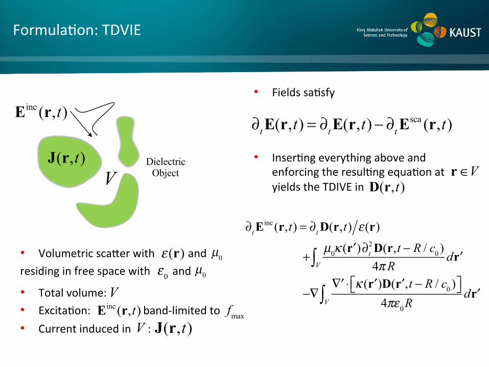
Einc (r,t)

µ0•  Volumetric sca[er with and residing in free space with and ε0 µ0

•  Total volume: •  Excita8on: band-‐limited to •  Current induced in :

V

Einc (r,t) fmax

J(r,t)

V J(r,t)

R = r − ′r

V

•  Fields sa8sfy

Dielectric

Object

Einc (r,t)

J(r,t) ∂t E(r,t) = ∂t E(r,t)− ∂t E

sca (r,t)

•  Inser8ng everything above and enforcing the resul8ng equa8on at yields the TDIVE in

∂t Einc (r,t) = ∂t D(r,t) ε(r)

+µ0κ ( ′r )∂t

2 D(r,t − R / c0 )4πR

d ′rV∫

−∇′∇ ⋅ κ ( ′r )D( ′r ,t − R / c0 )⎡⎣ ⎤⎦

4πε0Rd ′r

V∫

D(r,t) r ∈V

Formula8on: TDVIE

ε(r) µ0•  Volumetric sca[er with and residing in free space with and ε0 µ0

•  Total volume: •  Excita8on: band-‐limited to •  Current induced in :

V

Einc (r,t) fmax

V J(r,t)

•  To numerically solve the TDVIE •  Volume is divided into tetrahedrons •  is expanded as

•  Unknowns: •  Temporal basis func8ons: •  Spa8al basis func8ons:

D(r,t) ≅ I ′k , ′l T ′l (t)f ′k (r)

′l =0

N t

∑′k =1

NV

∑,k lI ′ ′

V

D(r,t)

f ′k (r)

f ′k (r) =±

Ak

3Vk± (r − r ′k

± ) , r ∈V ′k±

0 , elsewhere

⎧

⎨⎪

⎩⎪ nρ

+

nρ−

T ′l (t)

Formula8on: MOT Solu8on

Formula8on: Temporal Basis Func8on Selec8on

•  Lagrange interpola8on func8on (LIF) •  Wide spectrum (possible source of

instability) •  Discon8nuous deriva8ves (possible

source of instability)

•  Approximate prolate spheroidal wave func8ons (APSWF) •  Band-‐limited and short temporal

support •  Have con8nuous deriva8ves •  Non-‐causal

•  Non-‐causality is fixed by temporal extrapola8on !

•  Future values are predicted from past values

•  Tes8ng with at 8mes yields

•  How is this solved ? Solve for Solve for Solve for ….

Z0I l = Vl − Zl− ′l I ′l

′l =1

l−1

∑ − Zl− ′l I ′l′l =l+1

l+NminT −1

∑

{Zl− ′l }k , ′k = 1ε k (r)

fk (r) ⋅ f ′k (r)T ′l (lΔt)drVk

∫ +µ0

4πfk (r),κ ′k (r)f ′k (r),∂t

2T ′l (t)t=lΔt

+ 14πε0

∇⋅ fk (r),∇⋅ κ ′k (r)f ′k (r)⎡⎣ ⎤⎦ ,T ′l (t)t=lΔt

fk (r) lΔt

Z0I1 = V1 − Z−1I2 + Z−2I3

Z0I2 = V2 − Z1I1 − Z−1I3 − Z−2I4

Z0I3 = V3 − Z1I2 − Z2I1 − Z−1I4 − Z−2I5

I1

I2

I3

Formula8on: MOT Solu8on

Non-‐casual terms

Z0I1 = V1

Z0I2 = V2 − Z1I1

Z0I3 = V3 − Z1I2 − Z2I1

Extrapola8on

Formula8on: Temporal Extrapola8on

•  Harmonic Based Extrapola8on (HEBE) §  Assumes that the solu8on can be expanded in

terms of sine and cosine func8ons within the band of the excita8on

§  Expansion coefficients (amplitude of harmonics) are found using known past samples

§  Expansion is used to predict the future samples (extrapola8on)

•  Known to work well and produce stable results for weak sca[erers

•  Unstable for strong sca[ers •  Strong sca[erers support modes with decaying

and oscilla8ng components •  Frequency sampling cannot be accurately done

on the imaginary axis (i.e., sine/cosine approxima8on is not accurate)

•  Resonance modes of unit sphere

3rε = 6rε = 12rε =

Formula8on: Decaying and Oscillatory Modes

(2)1/21/2

(2)1/2 1/2

( / )( )( ) ( / )

n rn

n n r

HJJ H

ρ ερρ

βββ βρ ε

−−

+ +

=(2)1/21/2

(2)1/2 1/2

( / )( )( ) ( / )

n rn rr

n n r

Hn J nJ H

ρ ερ ε ερ ρ ρ

βρ ε

ββ β β β

−−

+ +

− = +

TE mode TM mode

•  Solu8on is expanded in terms of exponen8als :

•  Suppose that are known!

1A. Glaser and V. Rokhlin, “A new class of highly accurate solvers for ordinary differential equations,” J. of Sci. Comput., 38(3), pp. 368-399, March, 2009.

ϕ(t ) α ve

λvt

v=1

Nv

∑: complex numbers : weighting coefficients

λvα v

(v = 1...Nv )

λv

•  Extrapola8on coefficients:

•  Matrix rela8on:

•  Solu8on is found by minimum norm

least square solu8on

ϕ(t j)= {p}lϕ(t j−1+l−k)l=1

k∑

App=b

{b}v=eλvtk+1

{A p}ν ,l = eλνtl ; ν = 1,…,Nν ;

l = 1,…,k


•  Frequency sampling should be done on the complex frequency plane •  How to define a temporal extrapola8on ?

1A. Glaser and V. Rokhlin, “A new class of highly accurate solvers for ordinary differential equations,” J. of Sci. Comput., 38(3), pp. 368-399, March, 2009.

λv

maximum modulus principle

RRQR

minimum norm least square solution p

ϕ i = Aα

{A}ji=eλ jti, j=1,...,N ,

i=1,...,M

ϕ(t ) α ve

λvt

v=1

Nv

∑


•  How to find

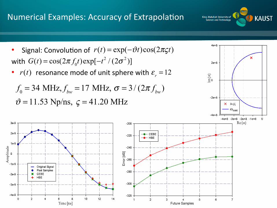
•  Signal: Convolu8on of with •  resonance mode of unit sphere with

r(t) = exp(−ϑt)cos(2πςt)

ε r = 12

Numerical Examples: Accuracy of Extrapola8on

G(t) = cos(2π f0t)exp[−t2 / (2σ 2 )]

r(t)

f0 = 34 MHz, fbw = 17 MHz, σ = 3/ (2π fbw )

ϑ = 11.53 Np/ns, ς = 41.20 MHz

rε

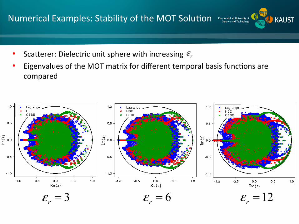
3rε = 6rε = 12rε =

Numerical Examples: Stability of the MOT Solu8on

•  Sca[erer: Dielectric unit sphere with increasing •  Eigenvalues of the MOT matrix for different temporal basis func8ons are

compared

•  Sca[erer: Dielectric shell •  , inner radius: 0.75m, outer radius 1m •  Excita8on:

ˆ ˆk = zˆ ˆp = x

3rε =

Numerical Examples: Accuracy of the MOT Solu8on

ε r = 3

Einc (r,t) = pG(t − tp − r ⋅ k / c)

G(t) = cos(2π f0t)exp[−t2 / (2σ 2 )]

f0 = 40MHz, fbw = 20MHz,σ = 3/ (2π fbw ), tp = 14σ

ˆ ˆk = z

ˆ ˆp = x

100rε =

•  Sca[erer: Dielectric shell •  , inner radius: 0.75m, outer radius 1m •  Excita8on:

ε r = 100

Einc (r,t) = pG(t − tp − r ⋅ k / c)

G(t) = cos(2π f0t)exp[−t2 / (2σ 2 )]

Numerical Examples: Accuracy of the MOT Solu8on

f0 = 18MHz, fbw = 9MHz, σ = 3/ (2π fbw ), tp = 14σ

•  Highlights: •  A highly stable TDVIE solver is formulated and implemented •  An extrapola8on scheme defined over the complex frequency plane helps to

achieve stability •  Numerical results demonstrate the accuracy and stability of the MOT solu8on on

high contrast sca[erers

•  Ongoing Work: •  Applying the TDVIE solver on realis8c structures •  Developing an explicit MOT scheme for solving the TDVIE

Conclusions and Future/Ongoing Work

Work Force PhD Students §  Muhammad Amin

§  Abdulla Desmal §  Ismail Uysal

§  Sadeed Sayed §  Noha Alharthi §  Ali Imran Sandhu

§  Ozum Asirim

Post-‐Doctoral Researchers

§  Kostyantyn Sirenko, PhD §  Arda Ulku, PhD §  Yifei Shi, PhD

§  Mohamed Farhat, PhD

Alumni

§  Mohamed Salem, PhD (Mar. 2013) §  Ahmed Al-‐Jarro, PhD (Nov. 2012) §  Meilin Liu, PhD (Jan. 2012)

§  Umair Khalid (MS degree, Dec. 2010) §  Muhammad Furqan (Feb. 2012)

§  Abdul Haseeb Muhammed (Apr. 2011)

Computa/onal Resources

Shaheen

§  IBM’s 16-‐Rack Blue Gene/P, ~65k compu8ng cores, 222 teraflops/sec

§  Expandable to petascale compu8ng

§  Supported by IBM and KAUST Supercompu8ng Laboratory (KSL)

Noor

§  Beowulf class heterogeneous cluster

§  Intel Xeon X5570, IBM Power6, ~1000 cores

§  Supported by KAUST Research Compu8ng

CEML: h[p://maxwell.kaust.edu.sa

KAUST Supercompu8ng Laboratory: h[p://www.hpc.kaust.edu.sa

CEM Research Group at KAUST – People and Facili8es

Applied Mathematics

Engineering

Computer Hardware/Software

CEM

Models, approximations, error

analysis Computational resources, new and specially designed architectures,

parallelization strategies, programming languages

Simulation Tools for Solving Maxwell Equations

Novel and robust formulations, fast

algorithms

Electromagnetics engineering applications

Multi-physics modeling and simulation frameworks: Coupled problems of structural, thermal,

and electromagnetic applications


Main objec8ve in CEM research: Developing efficient, rigorous, and accurate numerical methods for characterizing electromagne8c wave interac8ons on electrically large, mul8-‐scale, and realis8cally complex structures.

RecentAdvances&in&Numerical&Techniques&for& … seminars... · HFSS (FEM), Comsol (FEM), Many...

Documents

Transcript of RecentAdvances&in&Numerical&Techniques&for& … seminars... · HFSS (FEM), Comsol (FEM), Many...