Frugal Innovation, Sustainability, and Sustainable Frugal ...

8/6/2019 Reasoning the Fast and Frugal Way
http://slidepdf.com/reader/full/reasoning-the-fast-and-frugal-way 1/20
Psychological Review
1996, Vol. 103, No. 4,650-669Copyright 1996 by the American Psychological Association, Inc.
0033-295X/96/S3.00
Reasoning the Fast and Frugal Way: Models ofBounded Rationality
Gerd Gigerenzer and DanielG.GoldsteinMax Planck Institute for Psychological Research and University of Chicago
Humans and animals make inferences about the world under limited time and knowledge. Incon-
trast, many models of rational inference treat the mind as a Laplacean Demon, equipped with un-
limited time, knowledge, and computational might. Following H. Simon's notion of satisncing, the
authors have proposed a family of algorithms based on a simple psychological mechanism:one-
reason decision making. These fast and frugal algorithms violate fundamental tenets of classical
rationality: They neither look up nor integrate all information. Bycomputer simulation, the authors
held a competition between the satisncing"Take The Best" algorithm and various "rational" infer-
enceprocedures (e.g., multiple regression).The Take The Bestalgorithm matched or outperformed
all competitors in inferential speed and accuracy. This result is an existence proof that cognitive
mechanisms capable of successful performance in the real world do not need to satisfy the classical
normsofrational inference.
Organisms make inductive inferences. Darwin (1872/1965)
observed that people use facial cues, such as eyesthat waver and
lids that hang low, to infer a person's guilt. Male toads, roaming
through swamps at night, use the pitch of a rival's croak to infer
itssizewhen deciding whetherto fight (Krebs &Davies, 1987).
Stock brokers must make fast decisions about which of several
stocks to trade or invest when only limited information is avail-
able. The list goes on. Inductive inferences are typically based
on uncertain cues: The eyes can deceive, and so can a tiny toad
with adeepcroak in the darkness.
Howdoes an organism make inferences about unknown as-
pects of the environment? There are three directions inwhich
to look for an answer. From Pierre Laplace to George Boole to
Jean Piaget, many scholars have defended the nowclassical view
that the lawsofhuman inferenceare the laws ofprobabilityand
statistics (and to a lesser degree logic, which does not deal as
easily with uncertainty). Indeed, the Enlightenment probabi-
lists derived the laws of probability from what they believed to
bethe laws of human reasoning (Daston, 1988). Following this
time-honored tradition, much contemporary research in psy-
chology, behavioral ecology, and economics assumes standard
Gerd Gigerenzer and Daniel G. Goldstein, Center for Adaptive Be-
havior and Cognition, Max Planck Institute for Psychological Research,
Munich, Germany, and Department of Psychology. University of
Chicago.
This research was funded by National Science Foundation Grant
SBR-9320797/GG.
We are deeply grateful to the many people who have contributed to
thisarticle, includingHal Arkes, Leda Cosmides, Jean Czerlinski, Lor-
raine Daston, Ken Hammond, Reid Hastie, Wolfgang Hell, Ralph Her-
twig, Ulrich Hoffrage, Albert Madansky, Laura Martignon, Geoffrey
Miller, Silvia Papai, John Payne, Terry Regier, Werner Schubo, Peter
Sedlmeier, Herbert Simon, Stephen Stigler, Gerhard Strube, Zeno Swi-
jtink, John Tooby, William Wimsatt, and Werner Wittmann.
Correspondence concerning thisarticle should be addressed toGerd
Gigerenzer or Daniel G. Goldstein, Center for Adaptive Behavior and
Cognition, Max Planck Institute for Psychological Research, Leo-
poldstrasse 24, 80802 Munich, Germany. Electronic mail may be sent
via Internet to [email protected].
statistical tools to be the normative and descriptive models of
inference and decision making. Multiple regression, for in-
stance, is both the economist's universal tool (McCloskey,
1985) and a model of inductive inferencein multiple-cue learn-
ing (Hammond, 1990) and clinical judgment (B. Brehmer,
1994); Bayes's theorem is a model of how animals infer the
presenceofpredators or prey (Stephens&Krebs, 1986) aswell
as of human reasoning and memory (Anderson, 1990). This
Enlightenment view that probability theory and human reason-
ing are two sidesof the same coin crumbled in the early nine-
teenth century but has remained strong in psychology and
economics.
In the past 25 years, this stronghold came under attack by
proponents of the heuristics and biases program, who con-
cluded that human inference issystematically biased and error
prone, suggesting that the laws of inference are quick-and-dirty
heuristics and not the lawsof probability (Kahneman, Slovic,&
Tversky, 1982). This second perspectiveappearsdiametrically
opposed to the classical rationality of the Enlightenment, but
this appearance is misleading. It has retained the normative
kernel of the classical view. Forexample, adiscrepancy between
the dictates of classical rationality and actual reasoning is what
defines a reasoningerror in this program. Both viewsaccept the
lawsofprobabilityand statistics asnormative, but they disagree
about whether humans can stand up to these norms.
Many experimentshavebeen conducted to test the validity of
these two views, identifying a host of conditions under whichthe human mind appears more rational or irrational. But most
of this work hasdealt with simple situations, such asBayesian
inference with binary hypotheses, one single piece of binary
data, and all the necessary information conveniently laid out
for the participant (Gigerenzer & Hoffrage, 1995). In many
real-world situations, however, there are multiple pieces of in-
formation, which are not independent, but redundant. Here,
Bayes's theorem and other "rational" algorithms quickly be-
come mathematically complex and computationally intracta-
ble, at least for ordinary human minds. These situations make
neither of the two views look promising. If one wouldapply the
classical view to such complex real-world environments, this
650
8/6/2019 Reasoning the Fast and Frugal Way
http://slidepdf.com/reader/full/reasoning-the-fast-and-frugal-way 2/20
REASONING THE FAST AND FRUGAL WAY 651
would suggest that the mind is a supercalculator like a Lapla-
cean Demon (Wimsatt, 1976)—carrying around the collected
worksofKolmogoroff, Fisher, orNeyman—and simply needsa
memory jog, like the slave in Plato'sMeno. On the other hand,
the heuristics-and-biases view of human irrationality would
lead us to believe that humans are hopelessly lost in the face of
real-world complexity, given their supposed inability to reason
according to the canon of classical rationality, even in simple
laboratory experiments.
There is a third way to look at inference, focusing on the psy-
chological and ecological rather than on logic and probability
theory. This view questions classical rationality as a universal
norm and thereby questions the very definition of "good" rea-
soning on which both the Enlightenment and the heuristics-
and-biases views were built. Herbert Simon, possibly the best-
known proponent of this third view, proposed looking for
models of bounded rationality instead of classical rationality.
Simon (1956, 1982) argued that information-processing sys-
tems typically need tosatisfies rather than optimize. Satisficing,
a blend of sufficing and satisfying, is a word of Scottish origin,
which Simon uses to characterize algorithms that successfully
deal with conditions of limited time, knowledge, or computa-
tional capacities. His concept of satisficing postulates, for in-
stance, that an organism would choose the first object (a mate,
perhaps) that satisfies itsaspiration level—instead ofthe intrac-
table sequence of taking the time to survey all possible alterna-
tives, estimating probabilities and utilities for the possible out-
comes associated with each alternative, calculating expected
utilities, and choosing the alternative that scores highest.
Let us stress that Simon's notion of bounded rationality has
two sides, one cognitive and one ecological. As early as in Ad-
ministrativeBehavior(1945),he emphasized the cognitive lim-
itations of real minds as opposed to the omniscient Laplacean
Demons of classical rationality. Asearlyas in his Psychological
Review article titled "Rational Choice and the Structure of the
Environment" (1956), Simon emphasized that minds are
adapted to real-world environments. The two go in tandem:
"Human rational behavior is shaped by a scissors whose two
bladesare the structure of task environments and the computa-
tional capabilities of the actor" (Simon, 1990, p. 7). For the
most part, however, theories of human inference havefocused
exclusively on the cognitive side, equating the notion of
bounded rationality with the statement that humans are limited
information processors, period. In a Procrustean-bed fashion,
bounded rationality became almost synonymous with heuris-
tics and biases,thus paradoxically reassuring classical rational-
ity as the normative standard for both biases and bounded ra-
tionality (for a discussion of this confusion see Lopes, 1992).Simon's insight that the minds of living systems should be un-
derstood relative to the environment in which they evolved,
rather than to the tenets of classical rationality, has had little
impact so far in research on human inference. Simple psycho-
logical algorithms that were observed in human inference, rea-
soning, ordecision making wereoften discredited withouta fair
trial, because they looked so stupid by the norms of classical
rationality. For instance, when Keeney and Raifta (1993) dis-
cussed the lexicographic ordering procedure they had observed
in practice—a procedure related to the classofsatisficing algo-
rithms wepropose inthisarticle—they concluded that this pro-
cedure "is naively simple" and "will rarely pass a test of
'reasonableness'"(p. 78). Theydid not report such a test. We
shall.
Initially, the concept of bounded rationality wasonly vaguely
defined, often as that which is not classical economics, and one
could "fit a lot of things into it by foresight and hindsight," as
Simon (1992, p. 18) himself put it. We wish to do more than
oppose the Laplacean Demon view. We strive to come up with
something positive that could replace this unrealistic view of
mind. What are these simple, intelligent algorithms capable of
makingnear-optimal inferences?Howfast and howaccurate are
they? In this article, we propose a class of models that exhibit
bounded rationality in both ofSimon'ssenses. These satisficing
algorithms operate with simple psychological principles that
satisfy the constraints of limited time, knowledge, and compu-
tational might, rather than those of classical rationality. At the
same time, they are designed to be fast and frugal without a
significant loss of inferential accuracy, because the algorithms
can exploit the structure of environments.
The article isorganizedas follows. Webeginbydescribing the
task the cognitive algorithms are designed to address, the basic
algorithm itself, and the real-world environmenton which theperformance of the algorithm will betested. Next, wereport on
a competition in which a satisficing algorithm competes with
"rational" algorithms in making inferences about a real-world
environment. The "rational" algorithms start with an advan-
tage: They use more time, information, and computational
might to make inferences.Finally, westudy variants of the sati-
sficing algorithm that make faster inferences and get by with
even less knowledge.
The Task
Wedeal withinferential tasks inwhichachoice mustbe made
between two alternatives on a quantitative dimension. Considerthe following example:
Which city has a larger population?(a) Hamburg (b) Cologne.
Two-alternative-choice tasks occur in various contexts in which
inferences need to be made with limited time and knowledge,
such as in decision making and risk assessment during driving
(e.g., exit the highway now or stayon); treatment-allocationde-
cisions (e.g., who to treat first in the emergency room: the 80-
year-old heart attack victim or the 16-year-old car accident
victim); and financial decisions (e.g., whether to buy or sell in
the trading pit). Inference concerning population demograph-
ics, such as city populations of the past, present, and future
(e.g., Brown&Siegler, 1993), isof importance topeople work-ing in urban planning, industrial development, and marketing.
Population demographics, which is better understood than,say,
the stock market, will serve us later as a "drosophila" environ-
ment that allows us to analyze the behavior of satisficing
algorithms.
We study two-alternative-choice tasks in situations where a
person has to make an inferencebased solely on knowledge re-
trieved from memory. Werefer to this as inference from mem-
ory, as opposed to inference from givens. Inference from mem-
ory involves search in declarative knowledge and has been in-
vestigated in studies of, inter alia, confidence in general
knowledge (e.g., Juslin, 1994; Sniezek &Buckley, 1993); the
8/6/2019 Reasoning the Fast and Frugal Way
http://slidepdf.com/reader/full/reasoning-the-fast-and-frugal-way 3/20
652 G I G E R E N Z E R A N D GOLDSTEIN
effec t of repetition on belief (e.g., Hertwig, Gigerenzer, &Hoffrage, in press); hindsightbias(e.g., Fischhoff, 1977);quan-ti tative estimates of area an d population of nations (Brown &Siegler, 1993); and autobiographic memory of time(Huttenlocher, H edges, & Prohaska, 1988). Studies of infer-
ence from givens, on the other hand, involve making inference sfrom information presented by an experimenter (e.g., Ham-mond, Hursch, &Todd, 1964). In thetraditionofEbbinghaus's
nonsense syllables, attemptsare often made here toprevent in-
dividual knowledge from impacting on the results by usingproblems about hypothetical referents instead of actual ones.For instance, in celebrated judgment and decision-making
tasks, such as the "cab" problemand the"Linda"problem,all
the relevant information is provided by the experimenter, andindividual knowledge about cabsand hit-and-run accidents,or
feminist bank tellers, isconsidered of norelevance (Gigerenzer& Murray, 1987). A s a consequence, limited knowledge or in-dividual differences in knowledge play a small role in inferencefrom givens. In contrast, th e satisficing algorithms proposed inthis article perform inference from memory, they us e limited
knowledge as input, and as we will show, the y can actual ly profitfrom a lack of knowledge.
Assume t ha t a person does not know or cannot deduce the
answer to the Hamburg-Cologne question but needs to makean inductive inference from related real-world knowledge. H owis this inferenc e derived? How can we predict choice (Hamburg
or Cologne) from aperson'sstateofknowledge?
Theory
The cognitive algorithms we propose are realizations of aframework for modeling inferences from memory, th e t heoryo f probabilistic mental mo dels (PMM theory; se e Gigerenzer,1993; Gigerenzer, Hoffrage, & Kleinbolting, 1991). Th e t heoryof probabilistic mental models assumes that inferences aboutunkno wn states of the world are based on probability cues(Brunswik, 1955). Th e the ory relates thre e visions:(a ) Induc-tive in ference needs to be studied w ith respect to natural envi-ronme nts, as emphasized by Brunswik and Simon; (b) induc-tive inference iscarried out bysatisficing algorithms,as empha-sized by Simon; and (c) inductive inferences are based on
frequencies of events in a reference class, as proposed by Rei-chenbach and other frequentist statisticians. The theory of
probabilistic mental models accounts for choice and confi-
dence, but only choice isaddressed inthis article.
The major thrust of the theory is tha t i t replaces the canon ofclassical rationality with simple, plausible psychological mech-
anisms of in ference—mechanisms tha t a mind can actual lycarry out under limited time and knowledge and that could havepossibly arisen through evolution. Most traditional models ofinference, from linear multiple regression models to Bayesianmodels to neura l networks, try to f ind some optimal integrationof all informa tion available: Every bit of informat ion is takeninto account, w eighted, andcombined in acomputationally ex-
pensive w ay. The family of algorithms in PMM theory does no timplement this classical ideal. Search in memory for relevantinformation isreducedto aminimum, and there is no integra-tion (but ra ther a substitution)ofpiecesof information. Thesesatisficing algorithms dispense with the fiction of the omni-scient Laplacean Demon, who hasall the limeand knowledge
Recognition
Cuel
Cue 2
Cue 3Cue 4
Cue5
+
+
•
•
•
:::*::
::::*«:::
:::*::
+
:::̂ ::
:;;;$;:
; ; ; ; « ; ;
*
-
•
•
•
•
•
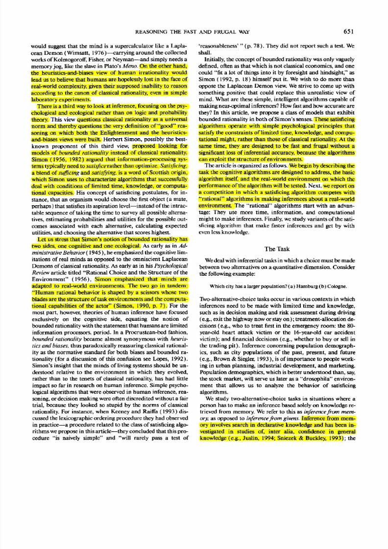
Figure 1, Illustration of bounded search through limited knowledge.Objects a, b, an d c ar e recognized; object rfis not. Cue values are posi-tive ( + ) or negative {-); missing knowledge is shown by questionmarks. Cues are ordered according to their validities. To infer whethera > b, th e Take The Best algorithm looks up only the cue values in theshaded space; to infer whether b > c, search is bounded to the dottedspace. The other cue values are not looked up.
to search for all relevant info rmat ion, to c ompute the weightsand covariances, and then to integrate all this informa tion intoan in fe rence ,
Limited Knowledge
A PMM is an inductive device that uses limited knowledge tomake fast inferences. Different from mental models of syllo-gisms and deductive inferenc e (Johnson-Laird, 1983), whichfocus on the logical task of tru th preservation and whe re knowl-edge is irrelevant (except for the meaning of connectives an dother logical te rms ), PMM s perform intelligent guesses about
unknown fe ature s of the w orld, based on unce rtain indicators.To make an infe rence about whic h of two objects, a or b, has ahigher value, knowledge about a reference class R is searched,with a, beK. In our exam ple, knowledge about the re fe renceclass "cities in Germany" could be searched. The knowledgeconsis tsof probabil ity cues C / (/ = I , . . . , « ) , andthecue valuesa/ and hi of the objects for the i t h cue . For instance, w hen mak-ing inferences about populations of Ge rman cities, the fact t h a ta city has a professional soccer team in the major league(Bundesliga) maycome to aperson's mind as a potential cue.That is,when considering pairsofGerman cities, if onecity has
a soccer team in the major league and theotherdoes not, thenth e ci ty wi th the team is likely, but not certain, to have the largerpopulation.
Limited knowledge means tha t th e matr ix of objects by cues
has missing entries (i.e., objects, cues, or cue values may beu n k n o w n ) . Figure 1 models th e limited knowledge of a person.Sh e has heard of three German ci t ies , a, b, and c, but not of
d (represented by thre e positive and one negative recognitionvalues). She know s some facts (cue values) about these citieswith respect to five binary cues. For a binary cue, there are twoc ue values, positive (e.g., the city hasa soccer team) or negative(i t does not). Positive refers to a cuevalue that signals ahighervalue on the target variable (e.g., having asoccer team iscorre-
lated with high population). Unknow n cue values are shown bya question mark. Because she has never heard of d, all cueval-ues for object f / a r e , by definition, unknown.
People rarely know all information on which an inference
8/6/2019 Reasoning the Fast and Frugal Way
http://slidepdf.com/reader/full/reasoning-the-fast-and-frugal-way 4/20
R E A S O N I N G T H E FAST A N D FRUGAL W A Y 653
could be based, that is, knowledge is limited. We model limited
knowledge in two respects: A person can have (a) incomplete
knowledge of the objects in the reference class (e.g., she recog-
nizes only some of the cities), (b) limited knowledge of the cue
values ( fac ts about cities), or (c) both. For instance, a person
who does not know all of the cities withsoccerteams may know
somecitieswith positive cue values (e.g., Munich and Hamburg
certainly haveteams),many with negative cuevalues(e.g., Hei-
delbergandPotsdam certainlydo not haveteams), andseveral
cities fo r whichc ue values willnot be known.
Th e Take Th e BestAlgorithm
The first satisficing algorithm presented is called the Take
Th e Best algorithm, because its policy is"take the best, ignore
therest."Itis thebasicalgorithm in the PMMframework. Vari-
ants that work faster or with less knowledge are described later.
We explain the stepsof the Take The Best algorithm for binary
c ue s (the algorithm can be easily generalized to many valued
cues), using Figure 1 for illustration.
TheTakeTheBest algorithm assumesasubjective rankorderof cues according to their validities (as in Figure 1). We call the
highest ranking cue (that discriminates between the two
alternatives) the best cue. The algorithm is shown in the form
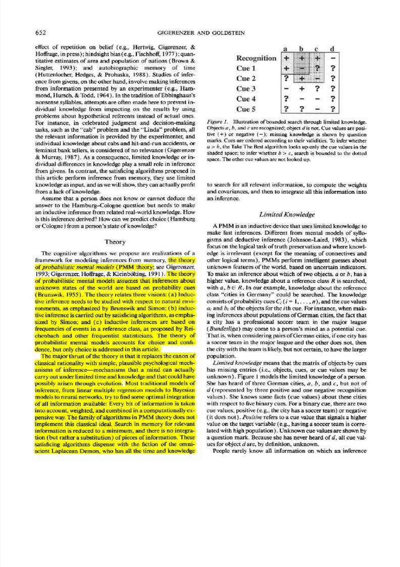
ofa flowdiagram inFigure 2.
Step 1: RecognitionPrinciple
Therecognition principle isinvoked whenthe mere recogni-
tion of an object is a predictor of the target variable (e.g.,
population). The recognition principle states the following: If
only one of the two objects is recognized, then choose the rec-
ognized object. If neither of the two objects is recognized, then
choose randomly between them. If both of the objects are rec-
ognized, thenproceedto Step2.Example: If a person in the knowledge state shown in Figure
Stan
Object a
positive unk nown negative
posit ive
Object b unknow n
negative
Figure 2. Flow diagramof the Take Th e Best algorithm.
Figure 3. Discrimination rule. A cue discriminates between two al-ternatives i f one has a positive c ue value and the other does not. Th efour d iscr imina t ing cases a re shaded.
1 is asked to in fe r wh ich of city a and city d has more inhabi-
tants, the in ference will be citya, because the person has never
heard of cityd before.
Step 2: Searchfor Cue Values
For the two objects, retrieve the cue values of the highest
rankingc ue from memory.
Step 3: Discrimination Rule
Decide whether the cue discriminates. The cue is said to dis-
criminate between two objects if one has a positive cue value
and the other does not. The four shaded knowledge states in
Figure 3 are those inwh ich a cue discriminates.
Step 4: Cue-Substitutio n Principle
If the cue discr iminates , then stop searchingfor cue values.Ifth e cue does not discriminate, go back to Step 2 and continue
with th e n ex t c ue untila c ue that discriminatesis found.
Step 5: Maximizing Rule o r Choice
Choose th e object with th e positive c ue value. If no cue dis-
cr iminates , then choose randomly.
Examples: Suppose th e task is judging whichof city a or b islarger (Figure I). Both cities are recognized (Step 1), and
search for the best cue results with a positive and a negative cue
value for Cue I (Step 2). The cue discriminates (Step 3), andsearch is terminated (Step 4). The person makes the inference
that citya islarger (Step 5).Suppose now the task is judging whichof cityb or c is larger.
Both citiesare recognized (Step 1), and search for the c ue val-
ues cue results in negativec ue value on object b for Cue 1, butth e corresponding c ue valuefor object c is unknown (S tep 2).
The cuedoesnot discriminate (Step 3), sosearch iscontinued
(Step 4). Search for the next cue results with positive and a
negative cue values for Cue 2 (Step 2). This cue discriminates
(Step3), and search is terminated (Step 4 ) . The person makes
th e inference that city b is larger (Step 5).
The features of this algorithm are (a) search extends through
only a portion of the total knowledge in memory (as shown by
the shaded and dotted partsof Figure 1) and isstopped imme-

8/6/2019 Reasoning the Fast and Frugal Way
http://slidepdf.com/reader/full/reasoning-the-fast-and-frugal-way 5/20
654 GIGERENZER AND GOLDSTEIN
diatelywhen the firstdiscriminating cue is found, (b) the algo-
rithm does not attempt to integrate information but uses cue
substitution instead, and (c) the total amount of information
processed is contingent on each task (pair of objects) and varies
in a predictable wayamong individuals with different knowl-
edge. This fast and computationally simple algorithm is a model
ofbounded rationality rather than ofclassicalrationality.There
is a close parallel with Simon's concept of "satisficing": The
Take The Best algorithm stops searchafter thefirstdiscriminat-
ing cue is found, just as Simon's satisficing algorithm stops
search after the first option that meetsan aspiration level,
The algorithm ishardly a standard statistical tool for induc-
tive inference: Itdoesnot use allavailableinformation, it isnon-
compensatory and nonlinear,and variantsof it can violate tran-
sitivity. Thus, it differs from standard linear tools for inference
such as multiple regression, as well as from nonlinear neural
networks that are compensatory in nature. The Take The Best
algorithm is noncompensatory because only the best discrimi-
nating cue determines the inference or decision; no combina-
tion of other cue values can overridethis decision. In thisway,
the algorithm does not conform to the classical economicviewof human behavior {e.g., Becker, 1976), where, under the as-
sumption that all aspects can be reduced to one dimension(e.g.,
money), there exists always a trade-off between commodities or
pieces of information. That is, the algorithm violates theArehi-
median axiom, which implies that for any multidimensional
object a(a,,a3,...,an) preferred tob(bt ,b2,.,.,£„),where
a, dominates b\, this preference can be reversed by taking
multiples of any one or a combinationof b2,b$,...,b,,. As we
discuss, variantsof this algorithm also violate transitivity, one
of the cornerstones of classical rationality (McCIennen, 1990).
Empirical Evidence
Despite their flagrant violation of the traditionalstandardsof
rationality, the Take The Best algorithm and other models from
the framework of PMM theoryhavebeensuccessful inintegrat-
ingvarious striking phenomena in inference from memory and
predictingnovel phenomena, such as the confidence-frequency
effect (Gigerenzer et al., 1991) and the less-is-more effect
(Goldstein, 1994; Goldstein & Gigerenzer, 1996). The theory
of probabilistic mental models seems to be the only existing
process theoryof the overconfidence bias that successfully pre-
dicts conditions underwhichoverestimation occurs, disappears,
and inverts to underestimation (Gigerenzer, 1993; Gigerenzer
et al., 1991; Juslin, 1993, 1994; Juslin, Winman, & Persson,
1995; but see Griffin & Tversky, 1992). Similarly, the theory
predicts when the hard-easy effect occurs, disappears, and in-verts—predictions that havebeen experimentallyconfirmedby
Hoffrage (1994)and by Juslin (1993). The TakeThe Bestalgo-
rithm explains also why the popular confirmation-bias expla-
nation of the overconfidence bias (Koriat, Lichtenstein, &
Fischhoff, 1980) is not supported by experimental data
(Gigerenzer etal., 1991, pp. 521-522).
Unlike earlier accounts of these striking phenomena in con-
fidence arid choice, the algorithms in the PMM framework al-
low for predictions of choice based on each individual'sknowl-
edge. Goldstein and Gigerenzer (1996) showed that the recog-
nition principle predicted individual participants" choices in
about 90% to 100% of all cases, even when participants were
taught information that suggested doing otherwise (negative
cue values for the recognized objects). Amongthe evidence for
the empirical validity of the Take-The-Best algorithm are the
tests of a bold prediction, the less-is-more effect, which postu-
latesconditions under which people with little knowledge make
better inferences than those who know more. This surprising
prediction has been experimentally confirmed. For instance,
U.S. students make slightly more correct inferences about Ger-
man citypopulations (about which they know little) than about
U.S. cities, and vice versa for German students (Gigerenzer,
1993; Goldstein 1994;Goldstein& Gigerenzer, 1995; Hoffrage,
1994). The theoryofprobabilistic mental models has been ap-
plied to other situations in which inferences have to be made
under limited time and knowledge, such as rumor-based stock
market trading (DiFonzo, 1994). Ageneral reviewof the theory
and its evidence is presented in McClelland and Bolger (1994).
The reader familiar with the original algorithm presented in
Gigerenzer et al.(1991) will have noticed that wesimplified the
discrimination rule.' In the present version, search is already
terminated if one object has a positive cue value and the other
does not, whereas in the earlier version, search wasterminatedonly whenoneobject had apositive valueand the other anega-
tive one (cf. Figure 3 in Gigerenzer et al. with Figure 3 in this
article). This change follows empirical evidence that partici-
pants tend to use this faster, simpler discrimination rule
(Hoffrage, 1994).
This article does not attempt toprovide further empirical ev-
idence. For the moment, weassume that the model isdescrip-
tively valid and investigatehow accurate this satisficing algo-
rithm is in drawing inferences about unknown aspects of a
real-world environment. Can an algorithm based on simple
psychological principles that violate the norms of classical ra-
tionality makea fair numberofaccurate inferences?
TheEnvironment
Wetested the performanceof the TakeThe Best algorithmon
how accurately it made inferencesabout a real-world environ-
ment. The environment was the set of all cities inGermany
with more than 100,000 inhabitants (83 cities after German
reunification), with population as the target variable. The
model of the environmentconsisted of 9binary ecological cues
and the actual 9X83 cue values.The fu l l model of theenviron-
ment isshown in theAppendix.
Each cue has an associated validity, which isindicative of its
predictive power. The ecological validity of a cue is the relative
frequency with which the cue correctly predicts the target, de-
finedwith respect to the reference class (e.g., all German citieswith more than 100,000 inhabitants). For instance, if one
checks all pairs in which one city has asoccer team but the other
city does not, one finds that in 87% of these cases, the citywith
the team also has the higher population. This value is the eco-
logical validityof the soccer team cue. The validity B ,- of the ith
cue is
», = p[t(a)> t(b)\ai ispositiveand b, isnegative],
1Also, we now use the term discrimination ruleinstead of activation
rule.

8/6/2019 Reasoning the Fast and Frugal Way
http://slidepdf.com/reader/full/reasoning-the-fast-and-frugal-way 6/20
REASONING THE FAST AND FRUGALWAY 655
Table 1
Cues,Ecological Validities, andDiscrimination Rates
Ecological Discrimination
Cue validity rate
National capital (Is the city the
national capital?)
Exposition site (Was the city once an
exposition site?)
Soccer team (Does the city havea team
in the major league?)
Intercity train (Is thecity on the
Intercity line?)
Statecapital (Isthe city a state capital?)
License plate (Is the abbreviation only
one letter long?)
University (Is the city home to a
university?)
Industrial belt (Isthe city in the
industrial belt?)
East Germany (Was the city formerly
in East Germany?)
1.00
.91
.87
.78
.77
.75
.71
.56
.51
.02
.25
.30
.38
.30
.34
.51
.30
.27
where t(a) and t(b) are the values of objects a and b on the
target variable t and p is a probability measured as a relative
frequency mR
The ecological validity of the nine cues rangedover the whole
spectrum: from .51 (only slightly better than chance) to 1.0
(certainty), as shown in Table 1. A cue with a high ecological
validity, however, is not often useful if its discrimination rate is
small.
Table 1 showsalso the discriminationratesfor each cue. The
discrimination rate of a cue is the relativefrequency withwhich
the cue discriminates between any two objects from the refer-
ence class. The discrimination rate is a function of the distribu-
tion of the cue valuesand the number N ofobjects in the refer-
ence class. Let the relativefrequencies of the positive and nega-
tivecuevaluesbex andy, respectively. Thenthediscrimination
rate dt of the j'th cue is
d,=-
as an elementary calculation shows. Thus, if N is very large,
the discrimination rate isapproximately 2xlyi .2The larger the
ecological validity of a cue, the belter the inference. The larger
the discrimination rate, the more often a cue can be used to
make an inference. In the present environment, ecological va-
lidities and discrimination rates are negatively correlated. The
redundancy of cues in the environment, as measured by pair-
wise correlations between cues, ranges between —.25 and .54,
with an averageabsolute value of.19.3
The Competition
The question of howwell a satisficing algorithm performs in
a real-world environment has rarely been posed in research on
inductive inference. The present simulations seem to be the first
to test howwell simple satisficing algorithms do comparedwith
standard integration algorithms, which require more knowl-
edge, time, and computational power. This question is impor-
tant for Simon's postulated link between the cognitive and the
ecological: If the simple psychological principles in satisficing
algorithmsare tuned toecological structures, these algorithms
should not fail outright.Weproposeacompetitionbetween var-
ious inferential algorithms. The contest will go to the algorithm
that scores the highest proportion of correct inferences in the
shortest time.
Simulating Limited Knowledge
We simulated people with varying degrees of knowledge
about cities in Germany. Limited knowledge can take two
forms. One is limited recognition of objects in the reference
class. The other is limited knowledge about the cue values of
recognized objects. To model limited recognition knowledge,
wesimulated people who recognized between 0 and 83 German
cities. Tomodel limitedknowledge of cue values, wesimulated
6 basic classes of people, who knew0%, 10%, 20%, 50%, 75%,
or 100% of the cue values associated with the objects theyrec-
ognized. Combining the two sources of limited knowledge re-
sulted in 6 x 84 types of people, each having different degrees
and kinds of limitedknowledge. Within each typeofpeople,we
created 500simulated individuals,whodiffered randomly from
one another in the particular objectsand cue values theyknew.
All objects and cue values known were determined randomly
within the appropriate constraints, that is, a certain number of
objects known, a certain total percentage of cue values known,
and the validity of the recognition principle (asexplained in the
following paragraph).
The simulation needed to be realistic in the sense that the
simulated peoplecould invokethe recognition principle. There-
fore, the setsofcities the simulated peopleknew had to be care-
fully chosen so that the recognized cities were larger than theunrecognized ones a certain percentage of the time. Weper-
formed a survey to get an empirical estimate of the actual co-
2For instance, if N = 2 and one cue value ispositive and the other
negative (x, = y, = .5), d, = 1.0. If A'increases, with x, and y, held
constant, then d, decreasesandconverges to 2x ty, .3There are various other measures of redundancy besides pairwise
correlation. The important point is that whatever measure of redun-
dancy one uses, the resultant value does not have the same meaning
for all algorithms. For instance, all that counts for the Take The Best
algorithm iswhat proportion of correct inferences the second cue adds
to the first in the cases where the first cue does not discriminate,how
much the third cue adds to the first two in the cases where they do not
discriminate, and so on. If a cue discriminates, search is terminated,
and the degree of redundancy in the cues that were not included in
the search isirrelevant. Integration algorithms, incontrast, integrateall
information and, thus, always work with the total redundancy in the
environment (or knowledgebase). For instance, when decidingamong
objects a,b,c,and din Figure 1, the cue values of Cues 3,4, and 5 do
not matter from the point of view of the Take The Best algorithm
(because search is terminated before reaching Cue 3). However, the
valuesof Cues3,4, and 5affect the redundancy of the ecological system,
froni the point of view of all integration algorithms. The lesson is that
the degree of redundancy in an environment depends on the kind of
algorithm that operates on the environment. One needs to be cautious
in interpreting measures of redundancy without reference to an
algorithm.

8/6/2019 Reasoning the Fast and Frugal Way
http://slidepdf.com/reader/full/reasoning-the-fast-and-frugal-way 7/20
656 G1GERENZER AND GOLDSTEIN
variationbetween recognition ofcitiesand city populations. Let
us define the validity a of the recognition principle to be the
probability, in a reference class, that one object has a greater
value on the target variablethananother, in the caseswhere the
one object isrecognized and the other isnot:
a =p[t(a)> t(b)\ a, is positive and b, isnegative],
where t(a) and t(b) are the values of objects a and b on the
target variablet,a, andb,are therecognition values of a and b,
andp is aprobability measuredas a relative frequency inJ?.
Inapilot studyof 26undergraduatesat theUniversity ofChi-
cago, we found that the cities they recognized (within the 83
largest inGermany) were larger than the cities theydid not rec-
ognize in about 80% of all possible comparisons. We incorpo-
rated this value into our simulationsbychoosing sets of cities
(for each knowledge state, i.e., for each number of cities
recognized) where the known cities were larger than the un-
known cities in about 80% of all cases. Thus, the cities known
bythe simulated individualshad the same relationship between
recognition and population as did those of thehuman individu-als. Let us first look at the performance of the Take The Best
algorithm.
Testing the Take The Best Algorithm-
We tested howwell individuals using the Take The Best algo-
rithmdid at answering real-world questions such as, Which city
hasmore inhabitants: (a) Heidelberg or (b) Bonn? Each of the
500simulated individualsineach of the 6 X 84 typeswastested
on the exhaustive set of 3,403 city pairs, resulting in a total of
500 X 6 X 84 X3,403tests, that is,about 858 million.
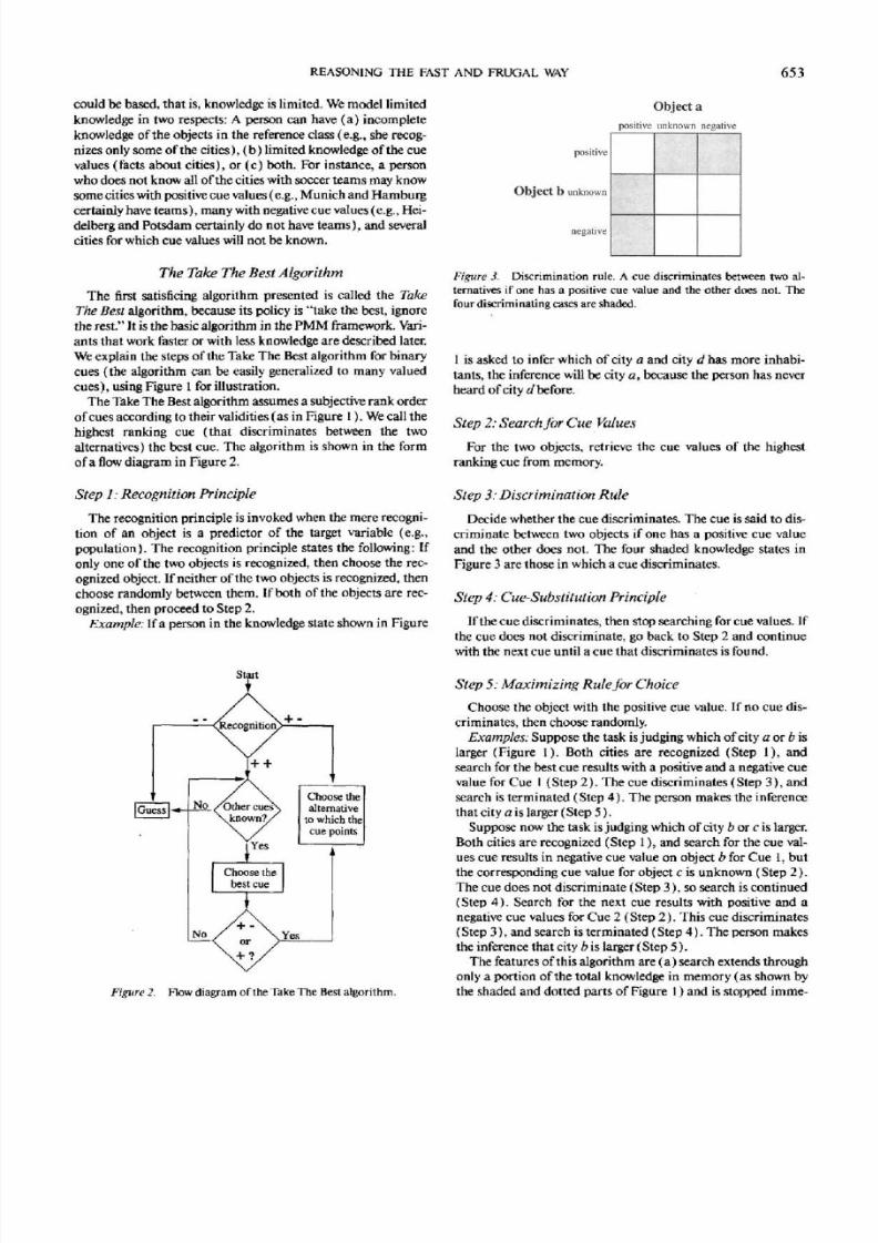
Thecurves inFigure 4 showtheaverage proportion ofcorrect
inferences foreach proportion ofobjects and cue valuesknown.
The x axis represents the number ofcities recognized, and the y
axis shows the proportion of correct inferences that the Take
The Best algorithm drew. Each of the 6 x 84points that make
up the sixcurves is an average proportion of correct inferences
taken from 500 simulated individuals, who each made 3,403
inferences.
When the proportion of cities recognized waszero, the pro-
portion of correct inferences was at chance level (.5). When up
to half of all cities were recognized, performance increased at
all levels of knowledge about cue values. The maximum per-
centage of correct inferences wasaround 77%.The striking re-
sult wasthat thismaximum was not achieved when individuals
knew all cue values of all cities, but rather when they knew less.
This result shows the ability of the algorithm to exploit limitedknowledge, that is, to do best when not everything isknown.
Thus, the Take The Best algorithm produces the less-is-mare
effect. At any level of limited knowledge of cue values, learning
more German cities will eventually cause adecrease in propor-
tion correct. Take, for instance, the curve where75% of the cue
values were known and the point where the simulated partici-
pants recognized about 60 German cities. If these individuals
learned about the remaining German cities, their proportion
correct would decrease. The rationale behind the less-is-more
e f f e c t is the recognition principle, and it can be understood best
from the curve that reflects 0% of total cue values known. Here,
alldecisions are made on the basis of the recognitionprinciple,
Percentage of Cue
Values Known
0 10 20 30 40 50 60 70 80
Number of Objects Recognized
Figure 4. Correct inferences about the population of German cities
(two-alternative-choice tasks) by the Take The Best algorithm. Infer-
ences are based on actual information about the 83 largest cities and
nine cues for population (seethe Appendix). Limited knowledge of the
simulated individuals isvaried across twodimensions: (a) the number
ofcitiesrecognized (xaxis) and (b) the percentageof cue valuesknown
(the sixcurves).
or by guessing. On this curve, the recognition principle comes
into play most when half of the cities are known, so it takes
on an inverted-U shape. When half the cities are known, therecognition principle can be activated most often, that is, for
roughly 50% of the questions. Because we set the recognition
validity in advance, 80% of these inferences will be correct. Tn
the remaining half of the questions, when recognition cannot
be used (either both cities are recognized or both cities are
unrecognized), then the organism is forced to guess and only
50%of the guesses will be correct. Usingthe 80%effective rec-
ognition validity half of the lime and guessing the other half of
the time, the organism scores 65%correct, which is the peak of
the bottom curve. The mode of this curve moves to the right
with increasing knowledge about cue values. Note that even
when a person knows everything, all cue values of all cities,
therearestates of limited knowledge inwhichthe person would
make more accurate inferences. We are not going to discuss
the conditions of this counterintuitive effect and the supporting
experimental evidence here (see Goldstein & Gigerenzer,
1996). Our focus is on howmuch better integration algorithms
can do in making inferences.
Integration Algorithms
We asked several colleagues in the fields of statistics and eco-
nomics todevise decision algorithms that would do better than
the Take The Best algorithm. The five integration algorithms
wesimulated and pitted against the TakeThe Best algorithm in
a competition were among those suggested by our colleagues.
8/6/2019 Reasoning the Fast and Frugal Way
http://slidepdf.com/reader/full/reasoning-the-fast-and-frugal-way 8/20
REASONING THE FAST AND FRUGAL WAY 657
These competitors include "proper" and "improper" linear
models(Dawes, 1979;Lovie&Lovie, 1986). Thesealgorithms,
in contrast to the Take The Best algorithm, embody two classi-
cal principles of rational inference: (a) complete search—they
use all available information (cuevalues)—and (b) complete
integration—they combine all these pieces of information into
a single value. In short, we refer in this article to algorithms
that satisfy these principles as "rational" (in quotation marks)
algorithms.
Contestant 1: Tallying
Let us start with a simple integration algorithm: tallying of
positive evidence (Goldstein, 1994). In this algorithm, the
number of positive cue values for each object is tallied across all
cues (;=!,...,«), and the object with the largest number
of positive cue values is chosen. Integration algorithms are not
based (at least explicitly) on the recognition principle. Forthis
reason, and to make the integration algorithms as strong as pos-
sible, we allow all the integration algorithms to makeuse of rec-
ognition information (the positive and negative recognition val-
ues, see Figure 1). Integration algorithms treat recognition as
a cue,like the nine ecological cues in Table 1. That is, in the
competition, the number of cues («) is thus equal to 10
(because recognition is included). The decision criterion for
tallying is the following:
If 2 < Z ; > 2 bi,then choose city a.
If2a* < Z 6< . then choose city b.
i=l j=I
If Z "i=
Z hi,then guess.
i= ] /- 1
The assignments of a, and b, are the following:
1 if the ;th cue value is positive
0 if the ;th cue value is negative
0 if the z'th cue value is unknown.
Let us compare cities a and b, from Figure 1. By tallying the
positive cue values, a would score 2 points and b would score 3.
Thus, tallying would choose b to be the larger, in opposition to
the Take The Best algorithm, which would infer that a is larger.
Variantsof tallying, such as the frequency-of-good-features
heuristic, have been discussed in the decision literature (Alba &
Marmorstein, 1987; Payne, Bettman,&Johnson, 1993).
Contestant 2: Weighted Tallying
Tallying treats all cues alike, independent of cue validity.
Weighted tallying of positive evidence is identical with tallying,
except that it weights each cue according to its ecological valid-
ity, t> , . The ecological validities of the cues appear in Table 1 .
We set the validity of the recognition cue to .8, which is the
empirical average determined by the pilot study. The decision
rule is as follows:
If 2 itVi > Z &№, then choose city a.
;-1 iHn n
If Z a,Vi < Z btv
t, then choose city b.
i-\ 1 - 1
If Z ofli = Z b,Vi, then guess,
i-i 1= 1Note that weighted tallying needs more information than either
tallying or the Take The Best algorithm, namely, quantitative
information about ecological validities. In the simulation, we
provided the real ecological validities to give this algorithm a
good chance.
Calling again on the comparison of objects a and b fromFig-
ure 1, let us assume that the validities would be .8 for recogni-
tion and .9, .8, .7, .6, .51 for Cues 1through?. Weighted tallying
would thus assign 1.7 points to a and 2.3 points to b. Thus,
weighted tallying would also choose b to be the larger.
Both tallying algorithms treat negative information and miss-
ing information identically. That is, they consider only positive
evidence. The following algorithms distinguish between nega-tive and missing information and integrate both positive and
negative information.
Contestant 3: Unit- Weight Linear Model
The unit-weight linear model is a special case of the equal-
weight linear model (Huber, 1989) and has been advocated as a
good approximation of weighted linear models (Dawes, 1979;
Einhorn & Hogarth, 1975). The decision criterion for unit-
weight integration is the same as for tallying, only the assign-
ment of a, and b, differs:
1 if the J th cue value is positive
— 1 if the fth cue value is negative
0 if the ith cue value isunknown.
Comparing objects a and b from Figure 1 would involve as-
signing 1.0 points to a and 1.0 points to b and,thus, choosing
randomly. This simple linear model corresponds to Model 2 in
Einhorn and Hogarth (1975, p. 177) with theweight parameter
set equal to 1.
Contestant 4: Weighted Linear Model
This model is like the unit-weight linear model except that
the values ofa, and b, are multipliedby their respective ecolog-
ical validities. The decision criterion is the same as with
weighted tallying. The weighted linear model (or some variant
of it) is often viewed as an optimal rule for preferential choice,
under the idealizationof independent dimensions or cues (e.g.,
Keeney & Raiffa, 1993; Payne etal., 1993). Comparing objects
a and b from Figure 1 would involve assigning 1.0 points to a
and 0.8 points to b and, thus, choosing a to be the larger.
Contestant 5: Multiple Regression
The weighted linear model reflects the different validities of
the cues, but not the dependencies between cues. Multiple re-
gression creates weights that reflect the covariances between
8/6/2019 Reasoning the Fast and Frugal Way
http://slidepdf.com/reader/full/reasoning-the-fast-and-frugal-way 9/20
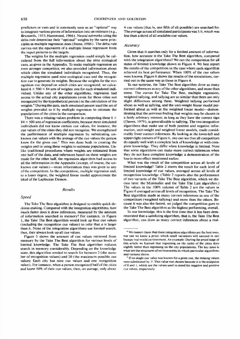
658 GIGERENZER AND GOLDSTEIN
predictors or cuesand is commonly seen as an "optimal"way
tointegrate various piecesof information intoanestimate(e.g.,
Brunswik, 1955;Hammond, 1966). Neural networks using the
delta rule determine their "optimal" weightsby the same prin-
ciples as multiple regression does (Stone, 1986). The delta rule
carries out the equivalent of a multiple linear regression from
the input patterns to the targets.
The weights for the multiple regression could simply be cal-
culated from the full information about the nine.ecological
cues, as given in the Appendix. To make multiple regression an
even stronger competitor, we also provided information about
which cities the simulated individuals recognized. Thus, the
multiple regression used nine ecological cues and the recogni-
tion cue to generate its weights. Because the weights for the rec-
ognition cue depend on which citiesare recognized, we calcu-
lated 6 X 500 X 84 sets of weights: one for each simulated indi-
vidual. Unlike any of the other algorithms, regression had
access to the actual city populations (even for those cities not
recognized by the hypothetical person) in the calculation of the
weights.4During the quiz, each simulated person used the set of
weights provided to it by multiple regression to estimate thepopulations of the cities in the comparison.
There was a missing-values problem incomputing these 6 X
84 x 500sets ofregression coefficients, because most simulated
individuals did not know certain cue values, for instance, the
cue values of the cities they did not recognize. We strengthened
the performance of multiple regression by substituting un-
known cue valueswith the average of the cue valuesthe person
knew for the given cue.5
This was done both in creating the
weights and in using these weights to estimate populations. Un-
like traditional procedures where weightsare estimated from
one half of the data, and inferences based on these weights are
made for the other half, the regression algorithm had access to
all the information in the Appendix (except, of course, the un-
known cue values)—more information than wasgiven to any
of the competitors. In the competition, multiple regression and,
to a lesser degree, the weighted linear model approximate the
ideal of the Laplacean Demon.
Results
Speed
The Take The Best algorithm is designed to enable quick de-
cision making. Compared with the integration algorithms, how
much faster does it draw inferences, measured by the amount
of information searched in memory? For instance, in Figure
1, the Take The Best algorithm would look up four cue values
(including the recognition cue values) to infer that a is larger
than b. None of the integration algorithms use limited search;
thus, theyalways look up all cue values.
Figure 5 shows the amount of cue values retrieved from
memory by the Take The Best algorithm for various levels of
limited knowledge. The Take The Best algorithm reduces
search in memory considerably. Depending on the knowledge
state, this algorithm needed to search forbetween 2 (the num-
ber of recognition values) and 20 (the maximum possible cue
values: Each city has nine cue values and one recognition
value). For instance, when a person recognized half of the cities
and knew 50% of their cue values, then, on average, only about
4 cue values (that is, one fifth of all possible)are searched for.
The average across all simulated participants was 5.9, which was
less than a third of all available cue values.
Accuracy
Given that it searches only for a limited amount of informa-
tion, how accurate is the Take The Best algorithm, compared
with the integration algorithms?We ran the competition for all
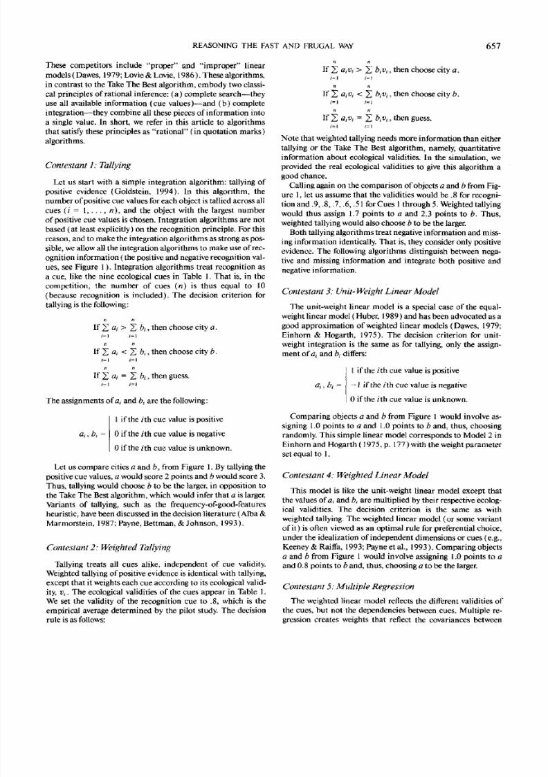
states of limited knowledge shownin Figure4. We first report
the results of the competition in the case where each algorithm
achieved its best performance: When 100% of the cue values
were known. Figure 6 shows the results of the simulations, car-
ried out in the same way as those inFigure 4.
To our surprise, the Take The Best algorithm drew as many
correct inferencesas anyofthe other algorithms, and more than
some. The curves for Take The Best, multiple regression,
weighted tallying, and tallying are so similar that there are only
slight differences among them. Weighted tallying performed
about as well as tallying, and the unit-weight linear model per-
formed about as well as the weighted linear model—demon-strating that the previous finding that weights may be chosen in
a fa ir ly arbitrary manner, as long as they have the correct sign
(Dawes, 1979), isgeneralizableto tallying. The two integration
algorithms that make use of both positive and negative infor-
mation, unit-weight and weighted linear models, made consid-
erably fewer correct inferences. Bylookingat the lower-left and
upper-right corners of Figure 6, one can see that all competitors
do equallywell withacomplete lackof knowledgeor with com-
plete knowledge. They d i f f e r when knowledge is limited. Note
that some algorithms can make more correct inferences when
they do not have complete knowledge: a demonstration of the
less-is-more effect mentioned earlier.
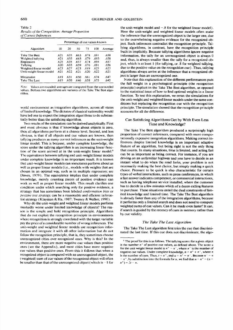
What was the result of the competition across all levels of
limited knowledge? Table 2 shows the result for each level of
limited knowledgeof cue values, averaged across all levels of
recognition knowledge. (Table 2 reports also the performance
of two variantsof the Take The Best algorithm, which wedis-
cuss later: the Minimalist and the Take The Last algorithm.)
The values in the 100% column of Table 2 are the values in
Figure 6 averaged across all levelsof recognition. The TakeThe
Best algorithm made as many correct inferences as one of the
competitors (weighted tallying) and more than the others. Be-
cause it was also the fastest, we judged the competition goes to
the Take The Best algorithm as the highest performing, overall.
To our knowledge, this is the first time that it has been dem-
onstrated that a satisficing algorithm, that is, the Take The Best
algorithm, can draw as many correct inferences about a real-
4Wecannot claim that these integration algorithms are the best ones,
nor can we know a priori which small variations will succeed in our
bumpy real-world environment. Anexample: During the proof stage of
this article we learned that regressing on the ranks of the cities does
slightly better than regressing on the city populations. The key issue is
what are the structures ofenvironments inwhich particular algorithms
and variants thrive.5
If no single cue value was known for a given cue, the missing values
were substituted by .5. Thisvaluewaschosen because it is the midpoint
of 0 and 1, which are the values used to stand for negative and positive
cue values, respectively.

8/6/2019 Reasoning the Fast and Frugal Way
http://slidepdf.com/reader/full/reasoning-the-fast-and-frugal-way 10/20
REASONING THE FAST AND FRUGALWAY 659
Percentage of Cue
Values Known
10 20 30 40 50 60 70
Number of Objects Recognized
80
Figure 5. Amount of cue values looked up by the Take The Best algorithm and by the competing integra-
tion algorithms (see text), depending on the number of objects known (0-83) and the percentage of cue
vuluesknown.
.75
IDU
°.65
•8
§I.55
Take The Best
Weighted Tallying
Tallying
Regression
Weighted Linear Model
Unit-Weight Linear Model
.75
.65
.55
0 10 20 30 40 50 60 70
Number of Objects Recognized
80
Figure 6. Results of the competition. The curve forthe Take The Best algorithm isidenticalwith the 100%
curve in Figure 4. The results for proportion correct havebeen smoothed by a running median smoother,
to lessen visual noise between the lines.
8/6/2019 Reasoning the Fast and Frugal Way
http://slidepdf.com/reader/full/reasoning-the-fast-and-frugal-way 11/20
660 GIGERENZER AND GOLDSTEIN
Table 2
Results of the Competition:Average Proportion
of Correct Inferences
Percentage of cue values known
Algorithm
Take The Best
Weighted tallying
Regression
Tallying
Weighted linear model
Unit-weight linear model
Minimalist
TakeThe Last
10
.621
.621
.625
.620
.623
.621
.619
.619
20
.635
.635
.635
.633
.627
.622
.631
.630
50
.663
.663
.657
.659
.623
.621
.650
.646
75
.678
.679
.674
.676
.619
.620
.661
.658
100
.691
.693
.694
.691
.625
.622
.674
.675
Average
.658
.658
.657
.656
.623
.621
.647
.645
A'o(t>. Valuesare rounded;averages are computedfrom the unrounded
values. Bottom two algorithms are variants of the Take The Best algo-
rithm.
world environment as integration algorithms, across all states
of limited knowledge.Thedictatesofclassical rationality would
have led one to expect the integration algorithmsto dosubstan-
tially better than the satisncingalgorithm.
Two results of the simulation can be derived analytically.First
and most obvious is that if knowledge about objects is zero,
then all algorithms perform at a chance level. Second, and less
obvious, is that if all objects and cue values are known, then
tallyingproduces as manycorrect inferences as the unit-weight
linear model. This is because, under complete knowledge, the
score under the tallying algorithm is an increasing linear func-
tion of the score arrived at in the unit-weight linear model.6
The equivalence between tallying and unit-weight linear models
under complete knowledge is an important result. It isknown
that unit-weight linear modelscan sometimes perform about as
well asproper linear models (i.e., models with weights that are
chosen in an optimal way, such as in multiple regression; see
Dawes, 1979). The equivalence implies that under complete
knowledge, merely counting pieces of positive evidence can
work as well as proper linear models. This result clarifies one
condition under which searching only for positive evidence, a
strategy that has sometimes been labeled confirmation bias or
positive test strategy, can be a reasonable and efficient inferen-
tial strategy (Klayman & Ha, 1987; Tweney&Walker, 1990).
Why do the unit-weight and weighted linear models perform
markedly worse under limited knowledge of objects? The rea-
son is the simple and bold recognition principle. Algorithms
that do not exploit the recognition principle in environments
where recognition isstrongly correlated with the target variable
pay the priceof aconsiderable numberof wrong inferences. The
unit-weight and weighted linear models use recognition infor-
mation and integrate it with all other information but do not
follow the recognition principle, that is. they sometimes choose
unrecognized cities over recognized ones. Why is this? In the
environment, there are more negative cue values than positive
ones (see the Appendix), and most cities have more negative
cue values than positive ones. From this it follows that when a
recognized object is compared with an unrecognized object, the
(weighted) sum of cuevaluesof the recognized object will often
be smaller than that of the unrecognized object (which is — 1 for
the unit-weight model and -.8 for theweighted linear model).
Here the unit-weight and weighted linear models often make
the inference that the unrecognized object is the larger one, due
to the overwhelming negative evidence for the recognized ob-
ject. Such inferences contradict the recognition principle. Tal-
lying algorithms, in contrast, have the recognition principle
built in implicitly. Because tallying algorithms ignore negative
information, the tally for an unrecognized object is always 0
and, thus, isalways smaller than the tally for a recognized ob-
ject, which is at least 1(for tallying,or .8 for weighted tallying,
due to the positive value on the recognitioncue).Thus, tallying
algorithms always arrive at the inference that a recognized ob-
ject is larger than an unrecognized one.
Note that thisexplanation of the different performances puts
the full weight in a psychological principle (the recognition
principle) explicit in the Take The Best algorithm, as opposed
to the statistical issue of how to find optimal weights in a linear
function. Totest this explanation, we reran the simulations for
the unit-weight and weighted linear models under the same con-
ditions but replacing the recognition cue with the recognition
principle. The simulation showed that the recognition principle
accounts for all the difference.
Can Satisficing Algorithms Get by With Even Less
Time and Knowledge?
The Take The Best algorithm produced a surprisingly high
proportion of correct inferences,compared with more compu-
tationally expensive integration algorithms. Making correct in-
ferences despite limited knowledge is an important adaptive
feature of an algorithm, but being right is not the only thing
that counts. In manysituations, time is limited, and acting fast
can be as important as being correct. For instance, if you are
driving on an unfamiliar highway and you have to decide in an
instant what to do when the road forks, your problem is not
necessarily making the best choice, but simply making a quick
choice. Pressure to be quick is also characteristic for certain
types ofverbal interactions, such aspressconferences, in which
a fast answer indicates competence,orcommercial interactions,
such as havingtelephone service installed, where the customer
has to decide in a fewminutes whichof a dozen calling features
to purchase. These situations entail thedual constraintsoflim-
ited knowledge and limited time. The Take The Best algorithm
is already faster than any of the integration algorithms, because
itperformsonly a limited search anddoes not need to compute
weighted sums of cue values. Can it bemadeeven faster? It can,
ifsearch is guided by the recency of cues in memory rather than
by cue validity.
The Take TheLast Algorithm
The TakeTheLast algorithmfirst triesthe cue that discrimi-
nated the last time. If this cue does not discriminate, the algo-
6The proof for thisis asfollows. The tallyingscore / for agiven object
is the number n+
of positive cue values, as defined above. The score u
for the unit weight linear model isn* - n~,where n~ is the numberof
negative cuevalues. Undercomplete knowledge,« - n+
+n~,wheren
isthenumber ofcues. Thus, t - n*,andu - n* - n~.Because n~ = n
- n +,bysubstitution into the formula foru,we findthat w = rt
+—(n —
8/6/2019 Reasoning the Fast and Frugal Way
http://slidepdf.com/reader/full/reasoning-the-fast-and-frugal-way 12/20
REASONING THE FAST AND FRUGALWAY 661
rithm then tries the cue that discriminated the time before last,
and so on. The algorithm differs from the Take The Best algo-
rithm in Step 2,which is now reformulated asStep 2':
Step 2': Search for the Cue Values of the
Most Recent Cue
For the two objects, retrieve the cue values of the cue used
most recently. If it is the firstjudgment and there is no discrim-
ination record available, retrieve the cue values of a randomly
chosen cue.
Thus, in Step 4, the algorithm goes back to Step 2'.Variants
of this search principle have been studied as the "Einstellung
effect" in the water jar experiments (Luchins & Luchins,
1994), where the solution strategy of the most recently solved
problem is tried first on the subsequent problem. This effect
has also been noted in physicians' generation of diagnoses for
clinical cases (Weber, Bockenholt, Hilton, &Wallace, 1993).
This algorithm does not need a rank order ofcues according
to their validities; all that needs to be known is the direction
in which a cue points. Knowledge about the rank order of cuevalidities isreplaced by a memory ofwhich cues were last used.
Note that such a record can be built up independently of any
knowledge about the structure of an environment and neither
needs, nor uses, any feedback about whether inferences are
right or wrong.
TheMinimalist Algorithm
Can reasonably accurate inferences be achieved with even
less knowledge? What we call the Minimalist algorithm needs
neither information about the rank ordering of cue validities
nor the discrimination history of the cues. In its ignorance, the
algorithm picks cues in a random order. The algorithm differs
from the Take The Best algorithm in Step 2, which is now re-
formulated as Step 2":
Step 2":Random Search
For the two objects, retrieve the cue values of a randomly
chosen cue.
The Minimalist algorithm does not necessarily speed up
search, but it tries to get by with even less knowledge than any
other algorithm.
Results
Speed
How fast are the fast algorithms? The simulations showed
that for each of the two variant algorithms, the relationship be-
tween amount of knowledge and the number of cue values
looked up had the same form as for the Take The Best algorithm
(Figure 5). That is, unlike the integration algorithms, the
curves are concave and the number of cues searched for is max-
imal when knowledge of cue values is lowest. The average num-
ber of cue values looked up was lowest for the Take The Last
algorithm (5.29) followed by the Minimalist algorithm (5.64)
and the Take The Best algorithm (5.91). As knowledge be-
comes more and more limited (on both dimensions: recogni-
tion and cue values known), the difference in speed becomes
smaller and smaller. The reason why the Minimalist algorithm
looks up fewer cue values than the Take The Best algorithm is
that cue validities and cue discrimination rates are negatively
correlated (Table 1); therefore, randomly chosen cues tend to
have larger discrimination rates than cues chosen by cue
validity.
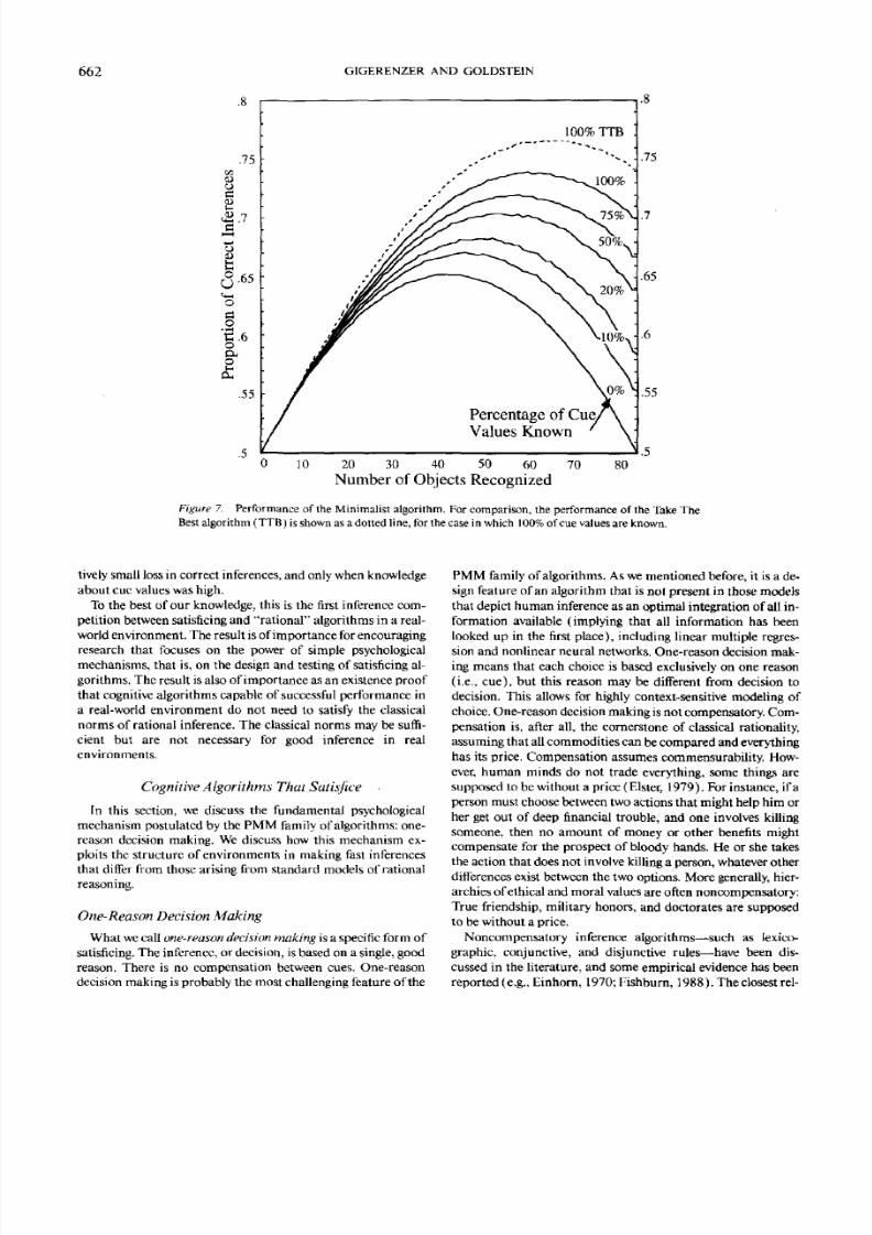
Accuracy
What is the price to be paid for speeding up search or reduc-
ing the knowledge of cueorderingsand discrimination histories
to nothing? We tested the performance of the two algorithms on
the same environment as all other algorithms. Figure 7 shows
the proportion of correct inferences that the Minimalist algo-
rithm achieved. For comparison, the performance of the Take
The Best algorithm with 100% of cue values knownis indicated
by a dotted line. Note that the Minimalist algorithm performed
surprisingly well. The maximum difference appeared when
knowledge wascomplete and all cities were recognized. Inthese
circumstances, the Minimalist algorithm didabout 4 percent-
agepointsworse than the TakeThe Best algorithm.On average,
the proportion of correct inferences was only 1.1 percentage
points less than the best algorithms in the competition (Ta-
ble 2).
The performance of the Take The Last algorithm is similar to
Figure 7, and the average number ofcorrect inferences isshown
in Table 2. The Take The Last algorithm wasfaster but scored
slightly less than the Minimalist algorithm. The Take The Last
algorithm hasan interesting ability, which fooled us in an earlier
series of tests, where weused asystematic (as opposed to a ran-
dom) method for presenting the test pairs, starting with the
largest city and pairingit with all others, and so on. An integra-
tion algorithm such as multiple regression cannot "find out"
that it is being tested in this systematic way, and its inferencesare accordingly independent of the sequence of presentation.
However, the TakeThe Last algorithm found out and wonthis
first round of the competition, outperforming the other com-
petitors by some 10percentage points. How did it exploit sys-
tematic testing? Recall that it tries, first, the cue that discrimi-
nated the last time. Ifthis cuedoes not discriminate, itproceeds
with the cue that discriminated the time before, and so on. In
doing so, when testing is systematic in the way described, it
tends to find, for each city that is beingpaired with all smaller
ones, the group of cues for which the larger city has a positive
value. Trying these cues first increases the chances of finding a
discriminating cue that points in the right direction (toward the
larger city). We learned our lesson and reran the whole compe-
tition with randomly ordered of pairs of cities.
Discussion
The competition showed a surprising result: The Take The
Best algorithm drew as many correct inferences about un-
known features of a real-world environment as any of the inte-
gration algorithms, and more than some of them. Two further
simplifications of the algorithm—the Take The Last algorithm
(replacingknowledge about the rank orders of cue validities by
a memory of the discrimination history of cues) and the Mini-
malist algorithm (dispensing with both) showed a compara-
8/6/2019 Reasoning the Fast and Frugal Way
http://slidepdf.com/reader/full/reasoning-the-fast-and-frugal-way 13/20
662 GIGERENZER AND GOLDSTEIN
.75.<D
g
0)
>
g
.65
o
o
(X
.55
100% TTB .
Percentage of Cue
Values Known
.75
.65
.55
0 10 20 30 40 50 60 70 80
Number of Objects Recognized
Figure 7. Performance of the Minimalist algorithm. For comparison, the performance of the Take The
Best algorithm (TTB) is shown as a dotted line, for the case in which 100%of cue valuesare known.
lively small loss in correct inferences, and only when knowledge
about cue valueswashigh.
To the best of our knowledge, this is the first inference com-
petition between satisficing and "rational" algorithms in a real-
world environment. The result isofimportance for encouraging
research that focuses on the power of simple psychological
mechanisms, that is, on the design and testing of satisficing al-
gorithms. The result isalsoof importance as an existence proof
that cognitive algorithms capable of successful performance in
a real-world environment do not need to satisfy the classical
norms of rational inference. The classical norms may be suffi-
cient but are not necessary for good inference in real
environments.
CognitiveAlgorithms That Satisfice
In this section, we discuss the fundamental psychological
mechanism postulated by the PMM family ofalgorithms: one-
reason decision making. We discuss how this mechanism ex-
ploits the structure of environments in making fast inferences
that differ from those arising from standard models of rational
reasoning.
One-Reason Decision Making
What we call one-reason decision making is a specific form of
satisficing. The inference, or decision, is based on a single, good
reason. There is no compensation between cues. One-reason
decision makingisprobably the most challenging featureof the
PMM family of algorithms. As wementioned before, it is a de-
sign feature of an algorithm that is not present in those models
that depict human inferenceas an optimal integration of all in-
formation available (implying that all information has been
looked up in the first place), including linear multiple regres-
sion and nonlinear neural networks. One-reason decision mak-
ing means that each choice isbased exclusivelyon one reason
(i.e., cue), but this reason may be different from decision to
decision. This allows for highly context-sensitive modeling of
choice. One-reasondecision making is not compensatory. Com-
pensation is, after all, the cornerstone of classical rationality,
assuming that allcommoditiescan becomparedandeverything
has its price. Compensation assumes commensurability. How-
ever, human minds do not trade everything, some things are
supposed to bewithout a price (Elster, 1979). For instance, if a
person must choose betweentwo
actions that might helphim or
her get out of deep financial trouble, and one involves killing
someone, then no amount of money or other benefits might
compensate for the prospect of bloody hands. He or she takes
the action that does not involve killinga person, whatever other
differences exist between the two options. More generally, hier-
archies of ethical and moral values are oftennoncompensatory:
True friendship, military honors, and doctorates are supposed
to bewithouta price.
Noncompensatory inference algorithms—such as lexico-
graphic, conjunctive, and disjunctive rules—have been dis-
cussed in the literature, and some empirical evidence has been
reported (e.g.. Einhorn, 1970;Fishburn, 1988). Theclosest rel-

8/6/2019 Reasoning the Fast and Frugal Way
http://slidepdf.com/reader/full/reasoning-the-fast-and-frugal-way 14/20
REASONING THE FAST AND FRUGAL WAY 663
ative to the PMM family of satisficing algorithmsis the lexico-
graphic rule. The largest evidence for lexicographic processes
seems to come from studies on decision under risk (for a recent
summary, see Lopes, 1995). However, despite empirical evi-
dence, noncompensatory lexicographic algorithms have often
been dismissed at face value because they violate the tenets of
classical rationality (Keeney & Raiffa, 1993; Lovie & Lovie,
1986).The PMM family is both more general and more specific
than the lexicographic rule. It is more general because only the
Take The Best algorithm uses a lexicographic procedure in
which cues are ordered according to their validity, whereas the
variant algorithms do not. It is more specific, because several
other psychological principles are integrated with the lexico-
graphic rule in the TakeThe Best algorithm, suchas the recog-
nition principle and the rules for confidence judgment (which
are not dealt with in thisarticle; see Gigerenzer et al., 1991).
Serious models that comprise noncompensatory inferences
are hard to find. One of the fewexamples is in Breiman, Fried-
man, Olshen, and Stone (1993), who reported a simple, non-
compensatory algorithm with only 3 binary, ordered cues,
which classified heart attack patients into high- and low-riskgroups and was more accurate than standard statistical classi-
fication methods that used up to 19 variables. The practical rel-
evance of this noncompensatory classification algorithm is ob-
vious: In the emergency room, the physician can quickly obtain
the measures on one, two, or three variables and does not need
to perform any computations because there is no integration.
This group of statisticians constructed satisficing algorithms
that approach the task of classification (and estimation) much
like the Take The Best algorithm handles two-alternative
choice. Relevance theory (Sperber, Cara, &Girotto, 1995) pos-
tulates that people generate consequences from rules according
to accessibility and stop this process when expectations of rele-
vance are met. Although relevance theory has not been as for-
malized, we see its stopping rule as parallel to that of the Take
The Best algorithm.Finally, optimality theory (Legendre, Ray-
mond, & Smolensky, 1993; Prince & Smolensky, 1991) pro-
poses that hierarchical noncompensation explains how the
grammarof a language determines which structural description
of an input best satisfies well-formedness constraints. Optimal-
ity theory (which is actually a satisficing theory) applies the
same inferential principles as PMM theory to phonologyand
morphology.
Recognition Principle
The recognition principle is a version of one-reason decision
making that exploits a lack of knowledge. The very fact thatone does not know is used to make accurate inferences. The
recognition principle is an intuitively plausible principle that
seems not to have been used until now in models of bounded
rationality. However, it has long been used to good advantage by
humans and other animals. For instance, advertisement tech-
niques as recently used by Benetton put all effort into making
sure that every customer recognizes the brand name, with no
effort made to inform about the product itself. The idea behind
this is that recognition is a strong force in customers' choices.
One of our dear (and well-read) colleagues, after seeing a draft
of this article, explained to us how he makes inferencesabout
which books are worth acquiring. If he finds a book about a
great topic but does not recognize the name of the author, he
makes the inference that it is probably not worth buying. If,
after an inspection of the references, he does not recognize most
of the names, he concludes the book is not even worth reading.
The recognition principle isalsoknown as one of the rules that
guide food preferences in animals. For instance, rats choose the
food that they recognizehavingeaten before (or havingsmelled
on the breath of fellow rats) and avoid novel foods (Gallistel,
Brown, Carey, Gelman, &Keil, 1991).
The empirical validityof the recognition principle for infer-
ences about unknown city populations, as used in the present
simulations, can be directly tested in several ways. First, partic-
ipants are presented pairs ofcities, among them critical pairs in
which one city isrecognized and the other unrecognized, and
their task is to infer which one has more inhabitants. The rec-
ognition principle predicts the recognized city. In our empirical
tests, participants followed the recognition principle in roughly
90% to 100%of all cases (Goldstein, 1994; Goldstein &Giger-
enzer, 1996). Second, participants are taught acue, its ecologi-
cal validity,and the cue values for some of the objects (such as
whether acityhas asoccer team or not). Subsequently, theyaretested on critical pairs of cities, one recognized and one unrec-
ognized, where the recognized city has a negative cue value
(which indicates lower population). The second test is a harder
test for the recognition principle than the first one and can be
made even harder byusing more cues with negativecue values
for the recognized object, and by other means. Testsof the sec-
ond kind have been performed, and participants still followed
the recognition principle more than 90% of the time, providing
evidence for its empirical validity (Goldstein, 1994; Goldstein
&Gigerenzer, 1996).
The recognition principle is a useful heuristic in domains
where recognition is a predictor of a target variable, such as
whether a food contains a toxic substance. In cases where rec-
ognition does not predict the target, the PMM algorithms can
still perform the inference, but without the recognition princi-
ple (i.e., Step 1 iscanceled).
Limited Search
Bothone-reasondecision makingand the recognition princi-
ple realize limited search bydefining stopping points. Integra-
tion algorithms, in contrast, do not provide any model of stop-
ping points and implicitly assume exhaustive search (although
they may provide rules for tossing out some of the variables in
a lengthy regression equation). Stopping rules are crucial for
modelinginference under limited time, as in Simon's examples
of satisficing, where search among alternatives terminates whena certain aspiration level is met.
Nonlinearity
Linearity is a mathematically convenienttool that hasdomi-
nated the theory of rational choice since its inception in the
mid-seventeenth century (Gigerenzer et al., 1989). The as-
sumption is that the various components of an alternative add
up independently to its overall estimate or utility. In contrast,
nonlinear inference does not operate by computing linear sums
of (weighted)cue values. Nonlinear inferencehasmany variet-
ies, including simple principles such as in the conjunctive and
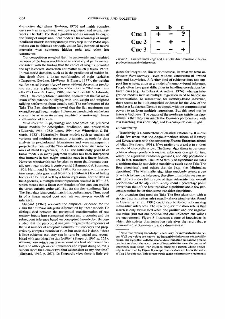
8/6/2019 Reasoning the Fast and Frugal Way
http://slidepdf.com/reader/full/reasoning-the-fast-and-frugal-way 15/20
664 GIGERENZER AND GOLDSTEIN
disjunctive algorithms (Einhorn, 1970) and highly complex
ones such as in nonlinear multiple regression and neural net-
works. The Take The Best algorithm and its variants belong to
the family ofsimple nonlinear models. Oneadvantageof simple
nonlinear models istransparency; every step in the PMM algo-
rithms can be followed through, unlike fully connected neural
networks with numerous hidden units and other free
parameters.
Our competition revealed that the unit-weightand weighted
versions of the linear models lead to about equal performance,
consistent with the finding that the choice of weights, provided
the sign is correct, does often not matter much (Dawes, 1979).
In real-world domains, such as in the prediction of sudden in-
fant death from a linear combination of eight variables
(Carpenter, Gardner, McWeeny & Emery, 1977), the weights
can be varied across a broad range without decreasing predic-
tive accuracy: a phenomenon known as the "flat maximum
effect" (Lovie & Lovie, 1986; von Winterfeldt & Edwards,
1982). The competition in addition, showed that the flat maxi-
mum effect extends to tallying, with unit-weight andweighted
tallying performingabout equally well. Theperformanceof theTake The Best algorithm showed that the flat maximum can
extendbeyond linearmodels: Inferences based solelyon the best
cue can be as accurate as any weighted or unit-weight linear
combination of all cues.
Most research in psychology and economics has preferred
linear models for description, prediction, and prescription
(Edwards, 1954, 1962; Lopes, 1994; von Winterfeldt & Ed-
wards, 1982). Historically, linear models such as analysis of
variance and multiple regression originated as tools for data
analysis in psychological laboratories and were subsequently
projected by means of the "tools-to-theories heuristic" intothe-
ories of mind (Gigerenzer. 1991). The sufficiently good fit of
linear models in many judgment studies has been interpreted
that humans in fact might combine cues in a linear fashion.
However, whether this can be taken to mean that humans actu-
ally use linear models is controversial (Hammond & Summers.
1965; Hammond &Wascoe, 1980). For instance, within a cer-
tain range, data generated from the (nonlinear) law of falling
bodies can be fitted well by a linear regression. For the data in
the Appendix,amultiple linear regression resulted inR2
- .87,
which means that a linear combination of the cues can predict
the target variable quite well. But the simpler, nonlinear, Take
The Best algorithm could match this performance. Thus, good
fit of a linear model does not rule out simpler models of
inference.
Shepard (1967) reviewed the empirical evidence for the
claim that humans integrate informationby linear models. Hedistinguished between the perceptual transformation of raw
sensory inputs into conceptual objects and properties and the
subsequent inference based on conceptual knowledge.He con-
cluded that the perceptual analysis integrates the responses of
the vast number of receptive elements into concepts and prop-
erties bycomplex nonlinear rules but once this isdone, "there
is little evidence that they can in turn be juggled and recom-
bined with anything like this facility" (Shepard, 1967. p. 263).
Although our minds can take account of a host of different fac-
tors, and although we can remember and report doing so, "it is
seldom more than one or two that weconsider at any one time"
(Shepard, 1967, p. 267). In Shepard's view, there is little evi-
a b
Cuel
Cue 2
Cue 3
Figure 8 Limited knowledge and a stricter discrimination rule can
produce intransitive inferences.
dence for integration, linear or otherwise, in what we term in-
ferences from memory—even without constraints of limited
time and knowledge. A further kind of evidence does not sup-
port linear integration as a model of memory-based inference.
People often have great difficulties in handling correlations be-
tween cues (e.g., Armelius& Armelius, 1974), whereas inte-
gration models such as multiple regression need to handle in-
tercorrelations. To summarize, for memory-based inference,
there seems to be little empirical evidence for the view of themind as a Laplacean Demon equipped with the computational
powers to perform multiple regressions. But this need not be
taken as bad news. The beauty of the nonlinear satisficingalgo-
rithms is that they can match the Demon's performance with
less searching, less knowledge, and lesscomputationalmight.
Intransitivity
Transitivity is a cornerstone of classical rationality. It is one
of the fewtenets that the Anglo-American school of Ramsey
and Savage shares with the competing Franco-European school
of Allais (Fishburn, 1991). If we prefer a to b and b toc, then
we should also prefer a to c. The linear algorithms in our com-
petition always produce transitive inferences (except for ties,
where the algorithm randomly guessed), and city populationsare, in fact, transitive. The PMM family of algorithms includes
algorithms that do not violate transitivity (such as the TakeThe
Best algorithm), and others that do (e.g., the Minimalist
algorithm). The Minimalist algorithm randomly selects a cue
on which to base the inference, therefore intransitivities can re-
sult. Table 2 shows that in spite of these intransitivities, overall
performance of the algorithm isonly about 1percentage point
lower than that of the best transitive algorithms and a few per-
centage points better than some transitive algorithms.
An organism that used the Take The Best algorithm with a
stricter discrimination rule (actually,the original version found
in Gigerenzer et al., 1991) could also be forced into making
intransitive inferences. The stricter discrimination rule is that
search is only terminated when one positive and one negative
cue value (but not one positive and one unknown cue value)
are encountered. Figure 8 illustrates a state of knowledge in
which this stricter discrimination rule gives the result that a
dominates b, bdominates c, andcdominates a.7
7Note that missing knowledge is necessary for intransitivtties to oc-
cur. If all cue values are known, no intransitive inferences can possibly
result. The algorithmwiththestricterdiscrimination rule allowsprecise
predictions about the occurrence of intransitivities over the course of
knowledge acquisition. For instance, imagine a person whose knowl-
edge isdescribed by Figure 8, except that shedoes not know the value
of Cue 2 for object c. Thisperson would make no intransitivejudgments
8/6/2019 Reasoning the Fast and Frugal Way
http://slidepdf.com/reader/full/reasoning-the-fast-and-frugal-way 16/20
REASONING THE FAST AND FRUGALWAY 665
Biological systems, for instance, can exhibit systematic in-
transitivities based on incommensurability between two sys-
temson one dimension(Gilpin, !975;Lewontin, 1968).Imag-
ine three species: a, b, andc.Species a inhabits both waterand
land; species b inhabits both water and air. Therefore, the two
onlycompete inwater, where speciesadefeats species b.Species
c inhabits land and air, so it only competes with b in the air,
where it is defeated by b. Finally, whena and c meet, it is only
on land, and here, c is in its element and defeats a. A linear
model that estimates some value for the combative strength of
each species independently of the species with which it is com-
peting would fa i l to capture this nontransitive cycle.
Inferences Without Estimation
Einhorn and Hogarth (1975) noted that in the unit-weight
model "there is essentially no estimation involved in its use" (p.
177), except for the sign of the unit weight. A similar result
holds for the algorithms reported here. The Take The Best algo-
rithm does not need to estimate regression weights, it only
needs to estimate a rank ordering of ecological validities. TheTake The Last and the Minimalist algorithms involve essen-
tially no estimation (except for the sign of the cues). The fact
that there is no estimation problem has an important conse-
quence: An organism can use as many cues as it has experi-
enced, without being concerned about whether the size of the
sample experienced issufficiently large to generate reliable esti-
mates of weights.
Cue Redundancy and Performance
Einhorn and Hogarth (1975) suggested that unit-weight
models can be expected to perform approximately as well as
proper linear models when (a) R2
from the regression model is
in the moderate or low range (around .5 or smaller) and (b)
predictors (cues) are correlated. Are these two criteria neces-
sary, sufficient, or both to explain the performance of the Take
The Best algorithm? The Take The Best algorithm and its vari-
ants certainly can exploit cue redundancy: If cues are highly
correlated, one cue can do the job.
We have already seen that in the present environment, R2
=
.87, which is in the high rather than the moderate nr low range.
As mentioned earlier, the pairwise correlations between the
nine ecological cues ranged between —.2 5 and .54, with an ab-
solute average value of .19. Thus, despite a high R2
and only
moderate-to-small correlation between cues, the satisficing al-
gorithms performed quite successfully. Their excellent perfor-
mancein thecompetition can beexplained only partiallyby cueredundancy, because the cues were only moderately correlated.
High cue redundancy, thus, does seem sufficient but is not nee-
comparing objects a, b, and c. If shewere to learn that object chad a
negative cue value for Cue 2, she would produce an intransitive judg-
ment. If she learned one piece more, namely, the value of Cue 1 for
object c, then she would no longer produce an intransitive judgment.
The prediction isthat transitive judgments should turn into intransitive
ones and hack, during learning.Thus, intransitivities do not simplyde-
pend on the amount of limited knowledge but also on what knowledge
ismissing.
essary for the successful performance of the satisficing
algorithms.
A New Perspective on the Lens Model
Ecological theorists such as Brunswik (1955) emphasized
that the cognitive system isdesigned to find many pathways to
theworld, substituting missing cues by whatever cues happen to
beavailable. Brunswik labeled this abilityvicarious functioning,
inwhich he saw the most fundamental principle of a science of
perception and cognition. Hisproposal to model this adaptive
process bylinear multipleregression has inspired a long tradi-
tion of neo-Brunswikian research (B. Brehmer, 1994; Ham-
mond, 1990), although the empirical evidence for mental
multiple regression isstill controversial (e.g., A. Brehmer& B.
Brehmer, 1988). However, vicarious functioning need not be
equated with linear regression. The PMM family of algorithms
provides an alternative, nonadditive model of vicarious func-
tioning, in which cue substitution operates without integration.
Thisgivesa newperspectiveofBrunswik's lens model. In a one-
reason decision making lens, the first discriminating cue thatpasses through inhibits any other rays passing through and de-
terminesjudgment. Noncompensatory vicariousfunctioning is
consistent with some of Brunswik's original examples, such as
the substitution of behaviors in Hull's habit-family hierarchy,
and the alternative manifestation of symptoms according to the
psychoanalyticwritings of Frenkel-Brunswik (see Gigerenzer &
Murray, 1987, chap. 3).
It has been reported sometimes that teachers, physicians, and
other professionals claim that they use seven or so criteria to
make judgments (e.g., when grading papers or making a differ-
ential diagnosis) but that experimental tests showed that they
in fact often used only one criterion (Shepard, 1967). At first
glance, this seems to indicate that thoseprofessionals make out-
rageous claims. But it need not be. If experts' vicarious func-
tioningworks according to the PMM algorithms, then they are
correct in sayingthat they use many predictors, but the decision
ismade byonlyone at any time.
What Counts as Good Reasoning?
Much of the research on reasoning in the last decades has
assumed that sound reasoning can be reduced to principles of
internal consistency, such as additivity of probabilities, confor-
mity to truth-table logic, and transitivity. For instance, research
on the Wason selection task, the "Linda" problem, and the
"cab" problem has evaluated reasoning almost exclusivelyby
some measure of internal consistency (Gigerenzer, 1995,1996a). Cognitive algorithms, however, need to meet more im-
portant constraints than internal consistency: (a) They need to
be psychologicallyplausible, (b) they need to be fast, and (c)
they need to make accurate inferences in real-world environ-
ments. In real time and real environments, the possibility that
an algorithm (e.g., the Minimalist algorithm) can make intran-
sitive inferences does not mean that it will make them all the
time or that this featureof the algorithm will significantly hurt
itsaccuracy. What we have not addressed in this article are con-
straints on human reasoning that emerge from the fact that
Homo sapiens is a social animal (Gigerenzer, 1996b). For in-
stance, some choices (e.g., who to treat first in an emergency

8/6/2019 Reasoning the Fast and Frugal Way
http://slidepdf.com/reader/full/reasoning-the-fast-and-frugal-way 17/20
666 GIGERENZER AND GOLDSTEIN
room) need to bejustified (Tetlock, 1992). Going with the sin-
glebest reason, the strategy of the TakeThe Best algorithm, has
an immediate appeal tor justification and can be more convinc-
ingand certainlyeasier tocommunicate than some complicated
weightingofcues.
further Research
Among the questions that need to be addressed in future re-
search are the following.First, how can we generalize the pres-
ent satisficing algorithm from two-alternative-choice tasks to
other inferential tasks, such as classification and estimation?
The reported success of the classification and regression tree
models (Breimanet al., 1993), whichuse a form of one-reason
decision making, is an encouraging sign that what we have
shown here for two-alternative-choice tasks might begeneraliz-
able. Second, what is the structure of real-world environments
that allows simple algorithms to perform so well? We need to
develop a conceptual language that can capture important as-
pects of the structureof environments that simple cognitiveal-
gorithms can exploit. The traditional proposal for understand-
ing the structureof environmentsin terms of ecological validi-
ties denned as linear correlations(Brunswik,1955) may not be
adequate, as the power of the nonlinear satisficing algorithms
suggests.
Can Reasoning Be Rational and Psychological?
At the beginningof this article,wepointed out the common
opposition between the rational and the psychological, which
emerged in the nineteenth century after the breakdown of the
classical interpretation of probability (Gigerenzeret al., 1989).
Since then, rational inference is commonly reduced to logic and
probability theory,andpsychological explanationsarecalled on
when things go wrong. This division of labor is, in a nutshell,
the basis on which much of the current research on judgment
under uncertainty isbuilt. As one economist from the Massa-
chusetts Instituteof Technology put it, "either reasoning is ra-
tional or it's psychological" (Gigerenzer, 1994). Can not rea-
soningbe both rational and psychological?
We believe that after 40 years of toying with the notion of
bounded rationality, it is time to overcome the opposition be-
tween the rational and the psychological and to reunitethe two.
The PMM family of cognitive algorithms provides precise
models that attempt to do so. They differ from the Enlighten-
ment's unified view of the rational and psychological, in that
they focus on simple psychological mechanisms that operate
under constraints of limited time and knowledge and are sup-
portedby empirical evidence. The singlemost important result
in thisarticleisthat simple psychological mechanismscanyield
about as many (or more) correct inferences in less time than
standard statistical linear models that embody classical proper-
ties ofrational inference. The demonstration that a fast and fru-
gal satisficing algorithmwon the competition defeats the wide-
spread view that only "rational" algorithms can be accurate.
Models of inference do not have to forsake accuracy for sim-
plicity. The mind can have it both ways.
References
Alba,J. W., &Marmorsiein. H. (1987).Theeffects of frequency knowl-
edge on consumer decision making. Journal of Consumer Research,
14. 14-26.
Anderson, J. R. (1990). The adaptive character of thought. Hillsdale,
NJ: Erlbaum.
Armelius, B., & Armelius, K. (1974). The use of redundancy in
multiple-cuejudgments: Data from a suppressor-variabletask.Amer-
icanJournal o f Psychology, 87, 385-392.
Becker. G. (1976). The economic approach to human behavior.Chi-
cago: Universityof Chicago Press.
Brehmer, A., & Brehmer, B. (1988). What have we learned about hu-man judgment from thirty years of policy capturing? In B.Brehmer
& C. R. B. Joyce (Eds.), Human judgment: The SJT view (pp. 75-
114). Amsterdam: North-Holland.
Brehmer, B. (1994). The psychology of linear judgment models. Aaa
Psych«logica,87, 137-154.
Breiman, L., Friedman, J. H., Olshen, R. A., &Stone, C. J. (1993).
Classification and regression trees. NewYork: Chapman &Hall.
Brown, N. R., &Siegler, R. S. (1993). Metrics and mappings: A frame-
work for understanding real-world quantitative estimation. Psycho-
logical Review, 100, 511-534.
Brunswik,E. (1955). Representative design and probabilistic theory in
a functional psychology.Psychological Review, 62, 193-217.
Carpenter, R.G.,Gardner, A., McWeeny, P. M., & Emery, J. L. (1977).
Multistage scoring system for identifying infants at risk of unex-
pected death.Archives of Disease in Childhood, S3, 606-612.
Darwin, C. (1965). Theexpressionsof theemotions in man and animal
Chicago: University of Chicago Press. (Original work published
1872)
Daston, L. (1988). Classical probability in the Enlightenment.
Princeton, NJ: Princeton University Press.
Dawes, R. M. (1979). The robust beauty of improper linear models.
American Psychologist, 34, 571-582.
DiFonzo, N. (1994). Piggybacked syllogisms for investor behavior:
Probabilistic mental modeling in rumor-based stock market trading.
Unpublished doctoral dissertation, TempleUniversity, Philadelphia.
Edwards, W.(1954).The theory of decision making. Psychological Bul-
letin. 51.3*0-411.
Edwards, W. (1962). Dynamic decision theory and probabilistic infor-
mation processing. Human Factors, 4,59-73.
Einhorn, H. J, (1970). The use of nonlinear,noncompensatorymodels
in decision-making.Psychological Bulletin, 73,221-230.
Einhorn, H. J., & Hogarth, R. M. (1975). Unit weighting schemes for
decision making.Organizational Behaviorand Human Performance,
13, 171-192.
Bister, J. (1979). Ulysses and the sirens: Studies in rationality and irra-
tionality. Cambridge, England: Cambridge University Press.
Fischer Welt Almanach [Fischer World Almanac]. (1993). Frankfurt,
Germany: Fischer.
Fischhoff, B. (1977). Perceived informativeness of facts. Journal o f Ex-
perimental Psychology: Human Perception and Performance, 3, 349-
358.
Fishburn, P. C. (1988). Nonlinear preference and utility theory. Balti-
more: Johns Hopkins University Press.
Fishburn, P. C. (1991). Nontransitive preferences in decision theory.Journal o f Risk and Uncertainty, 4, 113-134.
Gallistel, C. R., Brown, A. L., Carey, S., Gelman, R., & Keil, F. C.
(1991). Lessons from animal learning for the study of cognitive de-
velopment. In S.Carey& R. Gelman (Eds.), The epigenesis o f mind:
Essays on biology and cognition (pp. 3-36). Hillsdale, NJ: Erlbaum.
Gigerenzer, G. (1991). From tools to theories: A heuristic of discovery
in cognitive psychology. Psychological Revie*', 98, 254-267.
Gigerenzer, G. (1993). The bounded rationality ofprobabilistic mental
models. In K. I. Manktelow & D. E. Over (Eds.), Rationality: Psy-
chological and philosophical perspectives (pp. 284-313). London:
Routledge.
Gigerenzer, G. (1994). Why the distinction between single-event prob-
abilities and frequencies is relevant for psychology (andvice versa).
8/6/2019 Reasoning the Fast and Frugal Way
http://slidepdf.com/reader/full/reasoning-the-fast-and-frugal-way 18/20
REASONING THE FAST AND FRUGAL WAY 667
In G. Wright & P. Ayton (Eds.), Subjective probability (pp. 129-
161). New York:Wiley.
Gigerenzer, G. (1995). The taming of content; Some thoughts about
domains and modules. Thinking and Reasoning, 1, 324-333.
Gigerenzer, G. (1996a). On narrow norms and vague heuristics. A re-
ply to Kahneman and Tversky (1996). Psychological Review, 103,
592-596.
Gigerenzer, G. (1996b). Rationality:Why social context matters. In P.Baltes & U. M. Staudinger (Eds.), Interactive minds: Life-span per-
spectives on the social foundation of cognition (pp. 319-346). Cam-
bridge, England: Cambridge UniversityPress.
Gigerenzcr, G., &Hoffrage, U. (1995). How to improve Bayesian rea-
soning without instruction: Frequency formats. Psychological Re-
vim; 102. 684-704.
Gigerenzer. G., Hoffrage, U., &Kleinbolting, H. (1991). Probabilistic
mental models: A Brunswikian theory of confidence. Psychological
Review, 98, 506-528.
Gigerenzer, G.,&Murray,D. J. (1987). Cognition as intuitive statistics.
Hillsdale, NJ: Erlbaum.
Gigerenzer, G.,Swijtink, Z., Porter, T, Daston, L., Beatty, J., &Kriiger,
L. (1989). The empire of chance: How probability changed science
and everyday life. Cambridge, England: Cambridge UniversityPress.
Gilpin, M. E. (1975). Limit cycles in competition communities. TheAmerican Naturalist, 109. 51-60.
Goldstein. D. G. (1994). The less-is-more effect in inference. Unpub-
lished master's thesis, University of Chicago.
Goldstein, D. G., & Gigerenzer, G. (1996). Reasoning by recognition
alone: How toexploit a lack of knowledge. Unpublished manuscript.
Griffin, D., & Tversky, A. (1992). The weighing of evidence and the
determinants of confidence. Cognitive Psychology. 24, 411-435.
Hammond, K. R. (1966). The psychology of Kgon Bnmswik. New
York: Holt, Rinehart& Winston.
Hammond, K. R. (1990). Functionalism and illusionism: Can integra-
tion be usefully achieved? In R. M. Hogarth (Ed.), Insights in deci-
sion making(pp. 227-261).Chicago: UniversityofChicagoPress.
Hammond, K. R., Hursch. C. J., &Todd, F. J. (1964). Analyzing the
componentsof clinical inference. Psychological Review', 71,438-456.
Hammond, K. R., &Summers, D. A. (1965). Cognitive dependence on
linear and nonlinear cues. Psychological Review, 72, 215-244.
Hammond, K. R., & Wascoe, N. E. (Eds.). (1980). Realizations of
Brunswik's representative design: New directionsfor methodology of
social and behavioral science. San Francisco: Jossey-Bass.
Hertwig, R., Gigerenzer, G., &Horn-age, U. (in press). The reiteration
effect in hindsight bias.PsychologicalReview.
Hoffrage, U. (1994). Zur Angemessenheit subjektiver Sicherheits-Ur-
teile: Eine Exploration der Theorie der probabilistischen mentalen
Modelle [On the validity of confidence judgments: A study of the
theory ofprobabilisticmental models].Unpublished doctoral disser-
tation, Universitat Salzburg, Salzburg, Austria.
Huber, O. (1989). Information-processing operators in decision mak-
ing. In H. Montgomery & O. Svenson (Eds.), Process and structure
in human decision making(pp. 3-21). NewYork:Wiley.
Huttenlocher, J., Hedges, L., &Prohaska. V. (1988). Hierarchical orga-
nization in ordered domains: Estimating the datesof events. Psycho-
logical Review, 95,471-484.
Johnson-Laird, P. N. (1983). Mental models. Cambridge, MA: Har-
vard UniversityPress.
Juslin, P. (1993). An explanation of the hard-easy effect in studies of
realism of confidence in one'sgeneral knowledge. European Journal
oj CognitivePsychology, 5, 55-71.
Juslin, P.(1994). The overconfidence phenomenon as a consequence of
informal experimenter-guided selection ofalmanac items. Organiza-
tional Behavior and Human Decision Processes, 57, 226-246.
Juslin, P., Winman, A., & Persson, T. (1995). Can overconfidence be
used as an indicator ofreconstructive rather than retrieval processes?
Cognition. 54,99-130.
Kahneman, D.,Slovic, P., &Tversky,A. (Eds.). (1982). Judgment un-
der uncertainty: Heuristics and biases. Cambridge, England: Cam-
bridge UniversityPress.
Kecney, R. L., & Raiffa, H. (1993). Decisions with multiple objectives.
Cambridge, England: Cambridge UniversityPress.
Klayman. J., & Ha, Y. (1987). Confirmation, disconfirmation, and in-
formation in hypothesis testing. Psychological Review, 94,211-228.
Koriat, A., Lichtenstein, S., &Fischhoff, B. (1980). Reasonsfor confi-dence. Journal of Experimental Psychology: Human Learning and
Memory, 6, 107-118.
Krebs, J. R., & Davies, N. B. (1987). An introduction to behavioral
ecology(2nd ed.). Oxford: Blackwell.
Legendre, G., Raymond, W., & Smolensky, P. (1993). Analytic typol-
ogy of case marking and grammatical voice. Proceedingsof the Berke-
ley Linguistics Society. 19, 464-478.
Lewontin, R. C. (1968). Evolution ofcomplex genetic systems. In M.
Gerstenhaber (Ed.), Somemathematical questions in biology. Provi-
dence, RI: American Mathematical Society.
Lopes, L. L. (1992). Three misleading assumptions in the customary
rhetoric of the bias literature. Theory and Psychology, 2, 231 -236.
Lopes, L. L. (1994). Psychology and economics: Perspectives on risk,
cooperation, and the marketplace. Annual Review of Psychology. 45,
197-227.Lopes, L. L. (1995). Algebra and process in the modeling of risky
choice. In J. R. Busemeyer,R. Hastie, and D. Medin (Eds.), Decision
making from theperspective of cognitive psychology (pp. 177-220).
New York: Academic Press.
Lovie, A. D., & Lovie, P. (1986). The fiat maximum effect and linear
scoringmodels for prediction. Journal of Forecasting, 5. 159-168.
Luchins.A.S., &Luchins.E. H. (1994). Thewaterjar experiments and
Einstellungeffects: I. Earlyhistory and surveys oftextbook citations.
Gfstall Theory, I ft, 101-121.
McClelland, A. G. R.,&Bolger, F (1994). The calibration ofsubjective
probabilities: Theories and models 1980-1994. In G. Wright & P.
Ayton (Eds.), Subjective probability (pp . 453-482). Chichester, En-
gland: Wiley.
McClennen, E. F.(1990). Rationality and dynamic choice. Cambridge,
England: Cambridge UniversityPress.
McCloskey, D. N. (1985). The rhetoric of economics. Madison: Univer-
sity of Wisconsin Press.
Payne, J. W., Bettman, J. R., &Johnson, E. J. (1993). The adaptive
decision maker. Cambridge, England: Cambridge UniversityPress.
Prince, A., & Smolensky, P. (1991). Notes on connectionism and har-
mony theory in linguistics (Tech. Rep. No. CU-CS-533-91). Boulder:
University ofColorado, Department ofComputer Science.
Shepard. R. N. (1967). On subjectively optimum selections among
multi-attribute alternatives. In W. Edwards*A. Tversky (Eds.),De-
cision making(pp. 257-283).Baltimore: Penguin Books.
Simon, H. A. (1945). Administrative behavior: A study of decision-
making processes in administrative organization. New York: Free
Press.
Simon. H. A. (1956). Rational choice and the structureof the environ-
ment. Psychological Revim; 63, 129-138.
Simon, H. A. (1982). Models of bounded rationality. Cambridge, MA:
MIT Press.
Simon, H. A. (1990). Invariants of human behavior. Annual Review of
Psychology, 41, 1-19.
Simon, H. A. (1992). Economics, bounded rationality, and thecognitive
revolution. Aldershot Hants, England: Elgar.
Sniezek, J. A., &Buckley, T. (1993). Becoming more or less uncertain.
In N. J. Castellan (Ed.), Individual and group decision making (pp.
87-108). Hillsdale,NJ: Erlbaum.
Sperber, D., Cara, F., &Girotto, V. (1995). Relevance theory explains
the selection task. Cognition, 57, 31-95.
Stephens. D. W, & Krebs, J. R. (1986). Foraging theory. Princeton,
NJ: PrincetonUniversity Press.
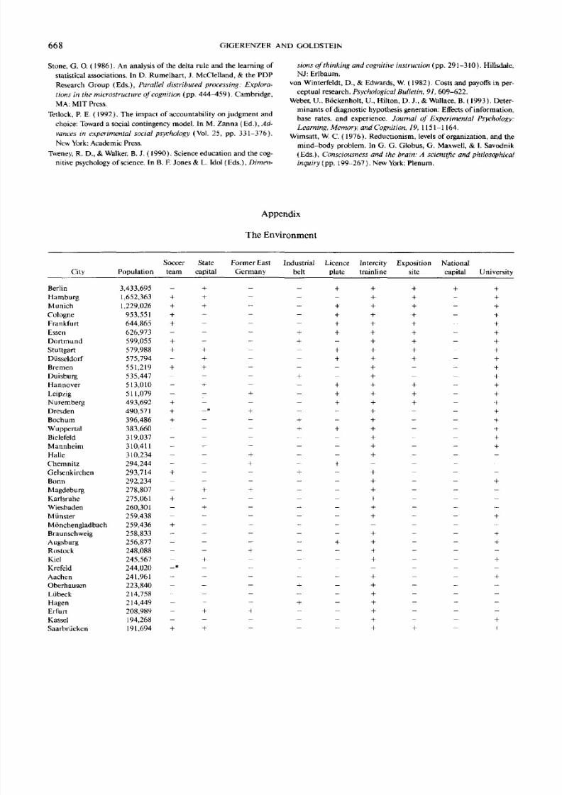
8/6/2019 Reasoning the Fast and Frugal Way
http://slidepdf.com/reader/full/reasoning-the-fast-and-frugal-way 19/20
668 GIGERENZER AND GOLDSTEIN
Stone, G. O. (1986). An analysis of the delta rule and the learning of
statistical associations. In D. Rumelhart, J. McClelland, & the PDF
Research Group (Eds.), Parallel distributed processing: Explora-
tions in the microstructure of cognition (pp. 444 1̂59). Cambridge,
MA: MIT Press.
Tetlock, P. E. (1992). The impact of accountability on judgment and
choice: Toward a social contingency model. In M. Zanna (Ed.), Ad-
vances in experimental social psychology (Vol. 25, pp. 331-376).
New York: Academic Press.
Tweney, R. D., &Walker. B. J. (1990). Science education and the cog-
nitive psychology of science. In B. F. Jones & L. Idol (Eds.), Dimen-
sions of thinking and cognitive instruction (pp. 291-310). Hillsdale,
NJ: Erlbaum.
von Winterfeldt, D., & Edwards, W. (1982). Costs and payoffs in per-
ceptual research. Psychological Bulletin, 91, 609-622.
Weber, U, Bockenholt, U., Hilton, D.J., &Wallace, B. (1993). Deter-
minants of diagnostic hypothesis generation: Effects of information,
base rates, and experience. Journal of Experimental Psychology:
Learning, Memory, and Cognition, 19, 1151-1164.Wimsatt, W. C. (1976). Reductionism, levels of organization, and the
mind-body problem. In G. G. Globus, G. Maxwell, & I.Savodnik
(Eds.), Consciousness and the brain: A scientific and philosophical
inquiry (pp. 199-267). NewYork: Plenum.
City
Berlin
Hamburg
Munich
Cologne
Frankfurt
Essen
Dortmund
Stuttgart
Diisseldorf
Bremen
Duisburg
Hannover
Leipzig
Nuremberg
Dresden
Bochum
Wuppertal
Bielefeld
Mannheim
Halle
Chemnitz
Gelsenkirchen
Bonn
Magdeburg
Karlsruhe
Wiesbaden
Miinster
Monchengladbach
Braunschweig
Augsburg
Rostock
Kiel
Krefeld
Aachen
Oberhausen
Lubeck
Hagen
Erfurt
Kassel
Saarbruckcn
Soccer State
Population team capital
3,433,695 - +
1,652,363 + +
1,229,026 4 +
953,551 +
644,865 4
626,973
599,055 4
579,988 + 4
575,794 - +
551,219 4 +
535,447
513,010
511,079
493,692 + -
490,57 1 + -*
396,486 4
383,660
319,037
310,411
310,234
294,244
293,714 +
292,234
278,807 - +
275,061 4
260,301 - +
259,438
259,436 4
258,833
256,877
248,088
245,567 - +
244,020 -*
241,961
223,840
214,758
214,449
208,989 - 4
194,268
191,694 + +
Appendix
The Environment
Former East Industrial Licence Intercity
Germany belt plate trainline
- - 4 4- - - +
+ +
- - 4 +- - 4 4+ 4 4- 4 - 4- - 4 4- - 4 4
- - — +- 4 - 4- - 4 ++ - 4 4
+ 4
4 - - +
- + - +
4 4 4
- -- - +- - 4+ - - 4
-I - t -- 4 - 4- - - +4 - - 4- - - t- - - +- - - 4
_- - - +- - 4 4+ - ~ 4_ _ _ +-- - - +
+ - +
- — — +
- + — +
-1 - — +- - - +- - - 4
Exposition National
site capital University
4 4 44 - 44 - 44 - 44 44 - 44 - 44 44 - 4- - 4— - H -4 - 44 - 44 - -1- - 4- - 4
4
- - - 4
4- - --- - -- - +- -- - -~ - 4- - -- - 4- — 4- - -- - 4-— — 4- - -- - -- - -- - -- — 4
+ - 1

8/6/2019 Reasoning the Fast and Frugal Way
http://slidepdf.com/reader/full/reasoning-the-fast-and-frugal-way 20/20
REASONING THE FAST AND FRUGALWAY 669
City
Freiburg
Hamm
Mainz
Hernc
Mtilheim
Solingen
Osnabriick
Ludwigshafen
Leverkusen
Neuss
Oldenburg
Potsdam
Darmstadt
Heidelberg
Bremerhaven
Gera
Wolfsburg
Wurzburg
Schwerin
Cottbus
Recklinghausen
Remscheid
Gottingen
Regensburg
Paderborn
Bottrop
Heilbronn
Offenbach
Zwickau
Salzgitter
Pforzheim
Ulm
Siegen
KoblenzJena
Ingolstadt
Witten
Hildesheim
Moers
Bergisch Gladbach
Reutlingen
Fiirth
Erlangen
Soccer State
Population team capital
191,029
179,639
179,486 - +
178,132
177,681
165,401
163,168
162,173
160,919 +
147,019
143,131
139,794 - +
138,920
136,796
130,446
129,037
128,510
127,777
127,447 - +
125,891
125,060
123,155
121,831
121,691
120,680
118,936
115,843
114,992
114,636
114,355
112,944
110,529
109,174
108,733105,518
105,489
105,403
105,291
104,595
104,037
103,687
103,362
102,440
Former East Industrial Licence Intercity Exposition National
Germany belt plate trainline site capital University
+ - - +
- + - + - - —- - - + - - +_ + _ _ _ _ _
_ + _ _ _ _ _- - + - - -- - - + - - +- - + - - -- _ _ _ _ _ _- - - - - - -- — — + — — +
+ - + + - - -
- - - + - - +- - - + - - +
_ _ _ - ) . _ _ _
+ - + + - - -_ _ _ _ _ _ _
- - - + - — +
+ - - + - - -+ _ _ _ _ _ _
+ - + - - -- _ _ _ _ _ _
- — — + - — +
- — + + - — +
- _ _ _ _ _ +
_ - ) . _ _ _ _ __ _ _ _ _ _ _
_ _ _ _ + _ _
+ - + - — - —_ _ _ _ _ _ _
_ _ _ . ( - _ _ _- - - + - - +_ _ _ _ _ _ +
- - - + - - ++ - + + - - +
- _ _ 4 _ _ _
_ + _ _ _ _ _
- - - + - — +
- + _ _ _ _ _
_ _ _ _ _ _ _- - - - - - -- _ _ + _ _ _- - + - - +
Note. City populations were taken from FischerWelt Almanack (1993).
* The twostarred minus values are, in reality, plus values. Because oftranscriptionerrors, we ran all simulations with these twominusvalues. These
do not affect the rank order of cue validities, should not haveany noticeable effect on the results, and are irrelevant for our theoretical argument.
Received May 20,1995
Revision received December 4,1995
Accepted December 8, 1995 •