Real-time Auto Tuning of a Closed Loop Second Order System ...

San Jose State University San Jose State University

SJSU ScholarWorks SJSU ScholarWorks

Master's Theses Master's Theses and Graduate Research

Fall 2013

Real-time Auto Tuning of a Closed Loop Second Order System Real-time Auto Tuning of a Closed Loop Second Order System

with Internal Time Delay Using Pseudo Random Binary Sequences with Internal Time Delay Using Pseudo Random Binary Sequences

David Adams San Jose State University

Follow this and additional works at: https://scholarworks.sjsu.edu/etd_theses

Recommended Citation Recommended Citation Adams, David, "Real-time Auto Tuning of a Closed Loop Second Order System with Internal Time Delay Using Pseudo Random Binary Sequences" (2013). Master's Theses. 4371. DOI: https://doi.org/10.31979/etd.x2vp-ab9a https://scholarworks.sjsu.edu/etd_theses/4371

This Thesis is brought to you for free and open access by the Master's Theses and Graduate Research at SJSU ScholarWorks. It has been accepted for inclusion in Master's Theses by an authorized administrator of SJSU ScholarWorks. For more information, please contact [email protected].

https://scholarworks.sjsu.edu/

https://scholarworks.sjsu.edu/etd_theses

https://scholarworks.sjsu.edu/etd

https://scholarworks.sjsu.edu/etd_theses?utm_source=scholarworks.sjsu.edu%2Fetd_theses%2F4371&utm_medium=PDF&utm_campaign=PDFCoverPages

https://scholarworks.sjsu.edu/etd_theses/4371?utm_source=scholarworks.sjsu.edu%2Fetd_theses%2F4371&utm_medium=PDF&utm_campaign=PDFCoverPages

mailto:[email protected]

REAL-TIME AUTO TUNING OF A CLOSED-LOOP SECOND-ORDER SYSTEM WITH

INTERNAL TIME-DELAY USING PSEUDO-RANDOM BINARY SEQUENCES

A Thesis

Presented to

The Faculty of the Department of Electrical Engineering

San José State University

In Partial Fulfillment

of the Requirements for the Degree

Master of Science

by

David M. Adams

December 2013

© 2013

David M. Adams

ALL RIGHTS RESERVED

The Designated Thesis Committee Approves the Thesis Titled



by

David M. Adams

APPROVED FOR THE DEPARTMENT OF ELECTRICAL ENGINEERING

SAN JOSÉ STATE UNIVERSITY

December 2013

Dr. Peter Reischl Department of Electrical Engineering

Dr. Ping Hsu Department of Electrical Engineering

Dr. Vitaly Spitsa Department of Electrical Engineering

ABSTRACT



by David M. Adams

This research yielded a real-time auto tuning algorithm to adaptively tune a

proportional integral and derivative (PID) controller for a first or second-order system with

internal time-delay. The method uses a 15-bit pseudo-random binary sequence as an input to

obtain the closed-loop system impulse response while the system is operating. Time-delay is

assessed by analysis of the estimated closed-loop impulse response and is used in the system

model for closed-loop pole assessment. The fast fourier transform of the estimated impulse

response produces an estimate of the frequency response data, and a non-linear regression

optimization technique, utilizing MATLAB, identifies the closed-loop system transfer

function based on assumed form. Closed-loop poles are then placed, based on an iterative

tuning study, automatically by the algorithm to achieve a user-defined overshoot and ensure

stability of the system with time-delay. This is accomplished by adjusting the PID

compensator gains. The algorithm is capable of tuning the system from an initially stable set

of PID gains to within 5% of the user-defined overshoot. The research demonstrates that the

auto tuning method is feasible for time-delays on the order of the plant time constant but is

extendable to larger time-delays.

v

ACKNOWLEDGEMENTS

This thesis was produced with the aid and support of many individuals that cannot all

be named. Without the support of dedicated faculty and unending support from friends and

family, this thesis would never have been complete. I would first like to thank my advisor

and mentor Dr. Peter Reischl for his inspirational guidance and support through the many

difficulties encountered during this research. I would like to thank Dr. Ping Hsu and Dr.

Vitaly Spitsa for providing excellent feedback and industry perspective which helped drive

the direction of the work. I would also like to thank my family and friends for their unending

support and prayers which motivated me to put my best work forward and allow for the

completion of this work. This thesis is dedicated to my loving wife Emily and my firstborn

son Nathan who sacrificed so much to give me the opportunity to continue my education.

vi

TABLE OF CONTENTS

1 Introduction 1

1.1 A Modern Perspective on Time-Delayed Systems 1

1.2 Traditional Methods for Dealing With Time-Delayed Systems 4

1.3 Motivation for Algorithm Development 6

2

Real-Time Auto Tuning Algorithm Development 9

2.1 Pseudo-Random Binary Sequences and Cross-Correlation Method Overview 11

2.2 System Identification of a Plant With Time-Delay 14

2.3 Compensator Tuning for the First-Order Plant With Time-Delay 18

2.4 Compensator Tuning for the Second-Order Plant With Time-Delay 26

2.5 Real-Time Gain Calculation for Systems With Time-Delay 31

3

Validation of the Cross-Correlation and System Identification Portions of the

Real-Time Auto Tuning Algorithm

40

3.1 First-Order PI Compensated Plant With Zero Time-Delay 40

3.2 Second-Order PID Compensated Plant With Zero Time-Delay 45

4

Results of Real-Time Auto Tuning Algorithm on Plants With Time-Delay 50

4.1 First-Order PI Compensated Plant With Normalized Time-Delay = 0.5 50

4.2 Second-Order PID Compensated Plant With Normalized Time-Delay = 0.5 56

4.3 First-Order PI Compensated Plant With Normalized Time-Delay = 1 61

4.4 Second-Order PID Compensated Plant With Normalized Time-Delay = 1 64

5

Conclusion 67

vii

6 Discussion 71

References

75

Appendices

Appendix A: Pseudo-Random Binary Sequence Generation for Real-Time Auto

Tuning

77

Appendix B: System Identification Routine Using MATLAB 79

Appendix C: Algorithm for Real-Time Auto Tuning With Time-Delay 81

viii

LIST OF FIGURES

Figure

Page

1

Example System Demonstrating Transport Lag, Modified

from (Ogata, 2002)

7

2 Algorithm Flow Diagram

9

3 Block Diagram Showing the System Overview and Its

Application to Time-Delayed Systems

10

4 Pseudo-Random Binary Sequence Generator and Output

Signals Modified from (Isermann & Münchhof, 2011)

12

5 Impulse Response of a Second-Order PID Compensated

System With Time-Delay (blue) Compared to the Time

Derivative of the Impulse Response (red)

15

6 Mean Square Error vs. Pole Parameter for a Second-Order

System With Time-Delay

18

7 Root Locus for First-Order PI Compensated Plant With

Normalized Time-Delay = 1 Generated Using Time-Delay

Exponential (Baker, 2011)

20

8 Root Locus for a First-Order PI Compensated Plant, With

Normalized Time-Delay = 0.5, Showing Closed-loop Poles

Being Drawn to the Left, Generated Using Time-Delay

Exponential (Baker, 2011)

22

9 Root Locus Plot for First-Order PI Compensated Plant, With

Normalized Time-Delay = 0.5, Utilizing the Compensator

Placement Method from Baker's Approach (2011), Generated

Using Time-Delay Exponential

23

10 Root Locus Plot for a First-Order PI Compensated System

With Normalized Time-Delay = 0.5, Showing Higher

Performance Generated Using Time-Delay Exponential

(Baker,2011)

25

ix

11 Root Locus Plot for Second-Order PID Compensated Plant

With Normalized Time-Delay = 0.5 and Compensator Zero

Placement Utilizing Baker Method (2011) Generated Using

Time-Delay Exponential

27

12 Root Locus for a Second-Order PID Compensated System

With Normalized Time-Delay = 0.5 Utilizing the Algorithm

Approach Generated Using Time-Delay Exponential

(Baker,2011)

29


With Normalized Time-Delay = 2 Utilizing the Baker Method

(2011) for Normalized Time-Delay = 0.5 Generated Using

Time-Delay Exponential

30


With Normalized Time-Delay = 2 Utilizing the Algorithm

Method Generated Using Time-Delay Exponential

(Baker,2011)

31

15 Step Response Examples for a First-Order PI Compensated

Plant With Normalized Time-Delay Values of 0.5, 1, and 2

36

16 Step Response Examples for a First-Order PI Compensated

Plant With Normalized Time-Delay Values of 0.5, 1, and 2

With a Slower Plant Pole

37

17 Step Response Examples for a Second-Order PID

Compensated Plant With Normalized Time-Delay Values of

0.5, 1, and 2

38

18 Step Response Examples for a Second-Order PID

Compensated Plant With Normalized Time-Delay Values of

0.5, 1, and 2 with a Slower Double Plant Pole

39

19 First-Order PI Compensated System With Zero Time-Delay

40

20 System Output for First-Order PI Compensated System With

Zero Time-Delay Due to Pseudo-Random Binary Sequence

Injection

42

21 Impulse Response Comparison between MATLAB impulse()

Function (blue) and Cross-Correlation Result (red) of a First-

Order PI Compensated System With Zero Time-Delay

43

x

22 Comparison of Bode Plot for Identified System (red) to Bode

Plot Data from Cross-Correlation (blue) for a First-Order PI

Compensated System With Zero Time-Delay

44

23 Second-Order PID Compensated System With Zero Time-

Delay

45

24 System Output for Second-Order PID Compensated System

With Zero Time-Delay Due to Pseudo-Random Binary

Sequence Injection

46

25 Impulse Response Comparison Between MATLAB impulse()

Function (blue) and Cross-Correlation Result (red) of a

Second-Order PID Compensated System With Zero Time-

Delay

47


Plot Data from Cross-Correlation (blue) of a Second-Order

PID Compensated System With Zero Time-Delay

48

27 First-Order PI Compensated Plant With Time-Delay

50

28 System Output for First-Order PI Compensated System With

Time-Delay Due to Pseudo-Random Binary Sequence

Injection

52

29 Estimated Impulse Response of a First-Order PI Compensated

System With Normalized Time-Delay = 0.5

53


Plot Data from Cross-Correlation (blue) of a First-Order PI

Compensated System With Normalized Time-Delay = 0.5

54

31 Step Response Outputs for a First-Order PI Compensated

Plant Tuned for Commanded Overshoots of 0, 5, 10, 15, and

20%

55

32 Second-Order PID Compensated Plant With Time-Delay

56

33 System Output for Second-Order PID Compensated System

With Time-Delay Due to Pseudo-Random Binary Sequence

Injection

57

xi

34 Estimated Impulse Response of a Second-Order PID

Compensated System With Normalized Time-Delay = 0.5

58


Plot Data from Cross-Correlation (blue) of a Second-Order

PID Compensated System With Normalized Time-Delay =

0.5

59

36 Step Response Outputs for a Second-Order PID Compensated

Plant Tuned for Commanded Overshoots of 0, 5, 10, 15, and

20%

60

37 First-Order PI Tuned Step Response for Normalized Time-

Delay = 1 (blue) and De-Tuned Response (green)

62

38 First-Order PI Compensated System With Oscillatory

Response (blue) and Re-Tuned Response (green)

63

39 Second-Order PID Tuned Step Response for Normalized

Time-Delay = 1 (blue) and De-Tuned Response (green)

65

40 Second-Order PID Compensated System With Oscillatory

Response (blue) and Re-Tuned Response (green)

66

xii

List of Tables

Table

Page

1

Recommended PI Tuning Relationships for a First-Order

Plant With Time-Delay

33

2 Recommended PID Tuning Relationships for a Second-

Order Plant With Time-Delay

34

1

1. Introduction

1.1 A Modern Perspective on Time-Delayed Systems

Time delay can have a pronounced effect on system operation. For the case of an

open-loop dynamic system, many real-world scenarios can influence the control response of

the system and cause the system to behave in a way that does not correspond to classical

analysis. In many cases, time-delayed systems are idealized and linearized around specific

operating regions to combat the time-delay effects (Ogata, 2002). Many examples of these

results are summarized by Sipahi, Niculescu, Abdallah, Michiels, and Gu (2011).

Before the advent of modern computing, handling time-delay in control system

design required special case design approaches that were very specific to the problem at hand

(Ogata, 2002). Pages of hand written calculations and validations were necessary to ensure

the design was valid and prototype work would then follow. Design iteration was often

required due to an un-modeled parameter that pushed the design out of the intended operating

limits. These control problems took many hours to develop mathematical approaches to solve

and resulted in designs that were ideal for specific operating conditions. If the conditions

were modified, the controller would have to be re-tuned or even re-designed altogether.

Large scale simulation packages have reduced the amount of iterative design required

for control problems. Today, any problem can be simulated with an advanced design

package. A model can be linear or non-linear, and the simulation software can run with any

initial condition, parameter, or model perturbation (Ogata, 2002). Although some of these

models are complicated, if there is time to build an accurate model and wait for the

simulation iterations to run, a solution that exemplifies what will occur when the system is

2

implemented can be attained. Even the waiting times for complex simulation runs are

becoming shorter as computational power increases. By analyzing the design in software, and

verifying the design for the range of known operating conditions, the designer can then

attempt the implementation in hardware with a better chance of proper control behavior

(Isermann & Münchhof, 2011).

The computational approach to design does not only extend to design simulations of

products prior to prototype. There is an increasing availability of small, off-the-shelf products

that provide users with advanced calculation ability (Miao, Zane, & Maksimovic, 2004).

Computationally intensive non-linear calculations and data analysis can be done on the fly

from a device that fits on a small prototype board, something that was unheard of a few short

years ago. These products can be leveraged to provide robust control solutions that are highly

capable, adaptive, and cheap to maintain.

Time-delayed systems do not follow classical control theory assumptions due to the

addition of phase caused by the time-delay exponential (Ogata, 2002). This phase change

causes the system to undergo a destabilizing effect as the time-delay increases. The negative

feedback process, under the influence of time-delay, inverts the output and feeds it back to

the input which causes an amplifying effect. This leads to an oscillatory response and is

followed by de-stabilization, which is due to the closed-loop poles moving into the right half

plane. This occurs, as was noted by Baker (2011) in his analysis of the time-delay Root

Locus, due to the creation of closed-loop poles from the time-delay exponential. As values of

the open loop gain increase, the time-delay poles migrate from far in the left half plane to

3

areas near the origin of the real axis. These poles repel the dominant closed-loop plant poles

into the right half plane, destabilizing the system.

The effect of the time-delay is a linear operator, as noted by Frazzoli (2010).

However, the analysis using more modern compensation approaches is computationally

intense. The idea of utilizing modern computing power to compensate for the effects of time-

delay needs to be researched and new techniques need to be developed to provide robust

compensation for time-delayed systems.

4

1.2 Traditional Methods for Dealing With Time-Delayed Systems

Time-delay is inherent in many process applications, and virtually all transport

process exhibit dead time (Vajta, 2000). The integration of computer systems into

compensation solutions also adds a time-delay to the system (Frazzoli, 2010). The effect of

this delay can become significant if it is even a small fraction of the system plant time

constant, which may be the case in a digital system. Time-delay can also be seen in systems

with solid state devices that require complex pulse width modulation. The switching time in

these devices can even introduce enough delay to cause instability in the system.

If the time-delay is sufficiently short, it can be ignored for the development of a

working controller. Engineers design the controller and are able to tune the controller, via

iterative methods, so the time-delay is compensated for properly. One method for iterative

tuning is referred to as the Ziegler-Nichols' method (1942). This method is good for a static

set of parameters and is sensitive to changes in time-delay. If the time-delay shifts, the

system can be driven towards instability.

Another common approach utilized to deal with time-delayed systems is a concept

that falls under modern control theory. System estimation is implemented in a specific

control application called a Smith Predictor (Bahill, 1983). This control scheme requires

good knowledge of the plant model and uses a simulated model that runs in tandem with the

actual plant. By utilizing feedback from the simulated model, the input error is adjusted and

the system is controlled as if there was no time-delay. If the time-delay estimate is inaccurate

or the time-delay changes, the predictor compensator is subject to the same weaknesses of

other static methods. Research has been conducted by Bahill (1983) into automatically

5

adjusting a Smith Predictor to utilize an updated time-delay. It is mentioned, however, that

this method must obtain an exact representation of the delay for proper operation. This

method allows for a larger gain to be maintained but requires a very accurate estimation of

the time-delay and system parameters.

Another commonly used approach is the approximation of the time-delay exponential

with a polynomial. This approximation is known as the Padé approximation and is based on

the Taylor expansion of the time-delay exponential (Vajta, 2000). In theory, by using higher

order terms of the Taylor expansion, the Padé approximation provides an estimate of the

time-delayed system that will better approximate the dynamics of the real system. This

allows for modeling of the system and design of controller parameters using standard root

locus methods (Frazzoli, 2010) to compensate for the time-delay. Being an approximation,

this approach is also subject to the same issues as the other methods that have been

mentioned. As time-delays shift, the approximation will no longer model the system

accurately and may even introduce additional error that makes the solution less accurate.

The most common approach to designing around time-delay is to ensure that the

system has an adequate phase margin to allow for the time-delay (Ogata, 2002). This

approach is based on the Bode Plot analysis of the open-loop system, and the design

approach utilizes compensator zeros to boost the phase of the system for higher frequencies.

Since the time-delay adds a negative phase to the system, the system is compensated to

ensure that the equivalent phase added by time-delay does not exceed the phase margin of the

system.

6

1.3 Motivation For Algorithm Development

This real-time auto tuning algorithm for time-delay systems was inspired by process

control problems in industry. The industry standard for process plant compensators relies on

the Proportional Integral and Derivative (PID) controller and 95% of the control loops for

process control are controlled via PID (Astrom & Hagglund, 1995). In many of these

systems liquids are heated and transferred from module to module during the process. The

fluids vary in temperature, flow, and pressure during the process which leads to complex

scenarios that are not always trivial to control. If the system has many operating states,

controller tuning will only be valid for a specific state or a range of states. If the system has

complex dynamics, including time-delay, the controller will require re-tuning for a change in

time-delay to meet the demand of the process.

A simple heater and air transfer system discussed in Ogata's text (2002) is shown in

Figure 1. This figure shows a hot air circulation system that transports heated air, through

ventilation ducts, to a room. The objective is to control the temperature of the room by

heating the air. In this case, the fuel source is governed by the temperature measured by the

thermometer. When the room temperature is too low, the furnace applies a heating input to

the system. There is a delay in transport of the heated air to the room, which causes a delay in

the temperature change in the room. The time-delay will be dependent primarily on the

blower speed, because it takes time for the air, traveling at velocity v, to travel the distance L.

This leads to a time-delay Td, given by

. The temperature output could be controlled with a

PID controller or a Smith Predictor (Bahill, 1983), but the system is simple enough to be

implemented and tuned for an adequate response without stressing the effects of time-delay.

7

Figure 1 - Example System Demonstrating Transport Lag, Modified from (Ogata, 2002)

This figure provides an example of time-delay. The air takes time to travel from the furnace to the room because

of the blower speed. The temperature feedback, for the furnace, is generated from a thermometer in the room. A

change in room temperature will cause a change in furnace output. The hotter or cooler air will not reach the

room for Td seconds. L refers to the length of the ventilation duct and v refers to the velocity of the air. This

delay in the observation of a change in the output variable is known as the transport delay and is primarily

dependent on blower speed.

There are numerous variables that can affect how this system operates and is

controlled. The temperature sensor could exhibit a time lag or a voltage offset, the furnace

could put in more or less heat depending on the temperature of the input air, and there are

heat losses from the ventilation ducts during transport of air to the room. These are all

examples of things that should be accounted for in the design and operation of the system.

Adequate models can be developed and a higher order control scheme can be implemented to

account for all of these effects.

One issue that has not been discussed is the flow of the air from the furnace to the

room. By an alteration of the air flow speed, v, the system will either be overcompensated or

8

undercompensated with respect to the original design specification. For an increase in the

time-delay, the furnace heats the air based on the current room temperature for Td seconds

with no change in room temperature. This heating is followed by a rapid rise in room

temperature, due to the hot air transfer through the ventilation ducts, so the furnace turns off.

The room stays overly hot for Td seconds, until the room begins to rapidly cool, due to no

furnace output. The furnace turns back on to raise the room temperature and the oscillatory

cycle repeats. The change in the time-delay has an oscillatory effect on the dynamics of the

system, and, if the time-delay is increased with a well compensated system, the system will

become unstable. In this case, the result was fluctuation in the output temperature causing

probable wear on the furnace and undesirable temperatures in the room.

9

2. Real-Time Auto Tuning Algorithm Development

This work illustrates a real-time PID auto tuning algorithm for time-delay systems.

The algorithm takes a commanded overshoot from the user and tunes the system to achieve

the overshoot. Once the overshoot is selected and delivered to the algorithm, the algorithm

will inject a frequency rich signal into the system, cross-correlate the input with the output to

achieve an estimate of the impulse response of the system, take the fast fourier transform

(FFT) (Oppenheim & Schafer, 2010) of the estimated impulse response to obtain the

estimated frequency response, identify the system transfer function based on known form

using a non-linear regression technique, and place the closed-loop plant poles to achieve the

desired overshoot in the system step response. This process is shown in Figure 2.

Figure 2 - Algorithm Flow Diagram

This flow diagram shows the steps in the algorithm. Each of these blocks represent a sub portion of the real-

time auto tuning algorithm. Although the cross-correlation method for system identification is not new (Miao et

al., 2004), this approach has not been applied to the tuning of systems with time-delay. Many of the methods,

shown in the blocks, are well studied but the application of placing the closed-loop poles based on the identified

system and time-delay has not been adequately addressed.

10

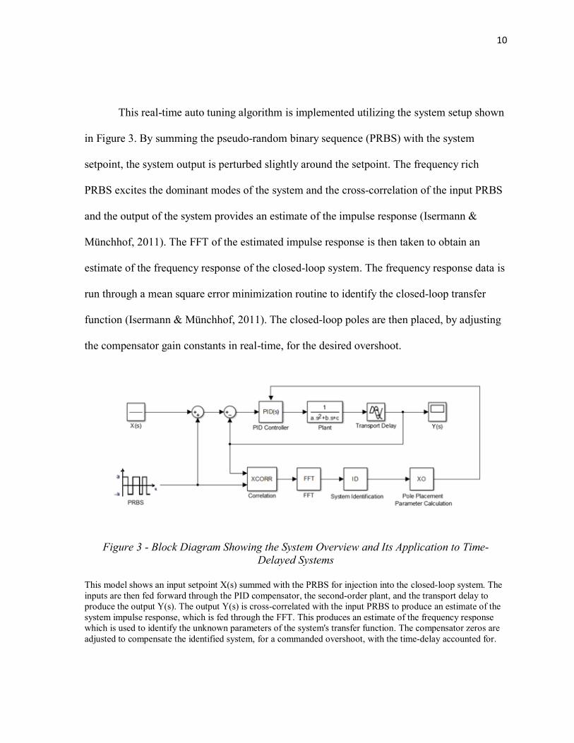
This real-time auto tuning algorithm is implemented utilizing the system setup shown

in Figure 3. By summing the pseudo-random binary sequence (PRBS) with the system

setpoint, the system output is perturbed slightly around the setpoint. The frequency rich

PRBS excites the dominant modes of the system and the cross-correlation of the input PRBS

and the output of the system provides an estimate of the impulse response (Isermann &

Münchhof, 2011). The FFT of the estimated impulse response is then taken to obtain an

estimate of the frequency response of the closed-loop system. The frequency response data is

run through a mean square error minimization routine to identify the closed-loop transfer

function (Isermann & Münchhof, 2011). The closed-loop poles are then placed, by adjusting

the compensator gain constants in real-time, for the desired overshoot.

Figure 3 - Block Diagram Showing the System Overview and Its Application to Time-

Delayed Systems

This model shows an input setpoint X(s) summed with the PRBS for injection into the closed-loop system. The

inputs are then fed forward through the PID compensator, the second-order plant, and the transport delay to

produce the output Y(s). The output Y(s) is cross-correlated with the input PRBS to produce an estimate of the

system impulse response, which is fed through the FFT. This produces an estimate of the frequency response

which is used to identify the unknown parameters of the system's transfer function. The compensator zeros are

adjusted to compensate the identified system, for a commanded overshoot, with the time-delay accounted for.

11

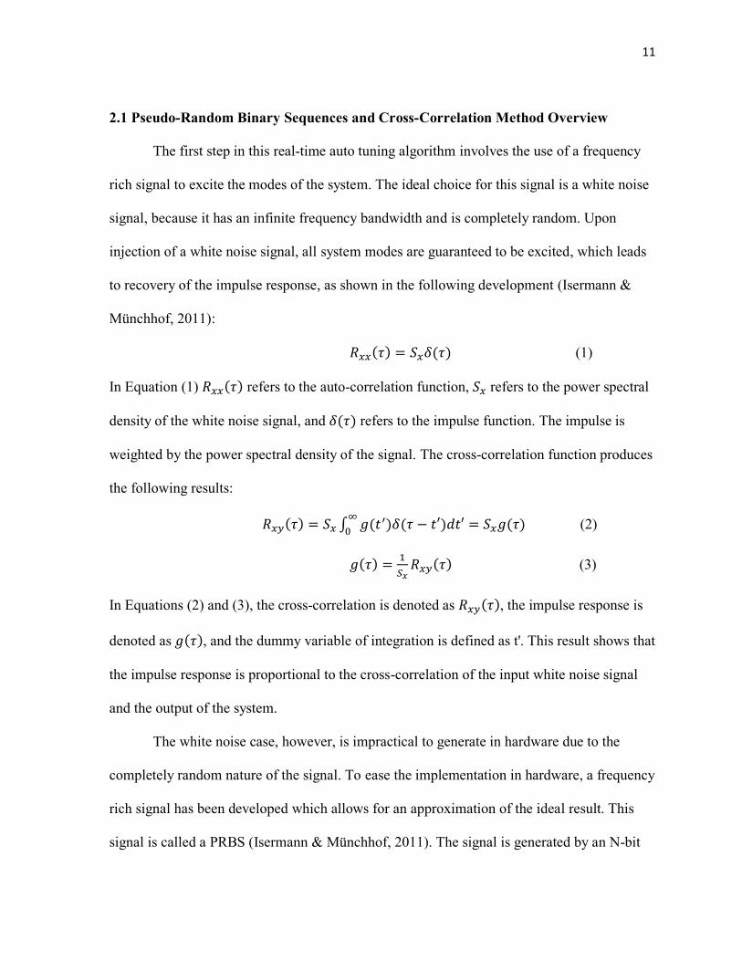
2.1 Pseudo-Random Binary Sequences and Cross-Correlation Method Overview

The first step in this real-time auto tuning algorithm involves the use of a frequency

rich signal to excite the modes of the system. The ideal choice for this signal is a white noise

signal, because it has an infinite frequency bandwidth and is completely random. Upon

injection of a white noise signal, all system modes are guaranteed to be excited, which leads

to recovery of the impulse response, as shown in the following development (Isermann &

Münchhof, 2011):

(1)

In Equation (1) refers to the auto-correlation function, refers to the power spectral

density of the white noise signal, and refers to the impulse function. The impulse is

weighted by the power spectral density of the signal. The cross-correlation function produces

the following results:

(2)

(3)

In Equations (2) and (3), the cross-correlation is denoted as , the impulse response is

denoted as , and the dummy variable of integration is defined as t'. This result shows that

the impulse response is proportional to the cross-correlation of the input white noise signal

and the output of the system.

The white noise case, however, is impractical to generate in hardware due to the

completely random nature of the signal. To ease the implementation in hardware, a frequency

rich signal has been developed which allows for an approximation of the ideal result. This

signal is called a PRBS (Isermann & Münchhof, 2011). The signal is generated by an N-bit

12

shift register that utilizes feedback from two of the shift register bits XOR'd together. If the

feedback registers are chosen properly, the shift register will cycle through 2N-1 states prior

to repeating a state. The binary output provided from the shift register is level shifted and

scaled to produce a zero mean output. This frequency rich signal exhibits a random nature

during a full cycle of the register values and produces a similar result to the ideal white noise

case (Isermann & Münchhof, 2011). An example PRBS generator is shown in Figure 4.

Figure 4 - Pseudo-Random Binary Sequence Generator and Output Signals Modified from

(Isermann & Münchhof, 2011)

This diagram shows the steps in generating a PRBS signal. The shift register is loaded with an initial starting set

of bits, a seed. Every clock cycle, the register shifts the bits to the right and the register receives a new bit from

the XOR operation. The output is level shifted to take the binary values and create a zero mean signal. This

signal is scaled by a value, a, to produce a signal that varies around zero, with an amplitude of a. It is important

to note that the output will be a time varying signal that is sufficiently random to be used as a system

identification tool (Isermann & Münchhof, 2011).

The development of this result can be seen in Isermann and Münchhof's work (2011),

and the resulting impulse response approximation is defined as follows:

(4)

In this case, a is the amplitude of the PRBS, is the sample time for the signal, and

is the cross-correlation of the input PRBS and the output of the system. As one can see, this

is a similar result with the impulse response being proportional to the cross-correlation. This

13

method has been successfully applied to complex systems such as a DC-DC converter in

research performed by Miao et al. (2004). A few notes about this result are that the

relationship shown in Equation (4) is an approximation of the actual behavior. The resulting

equation is based on the assumption that the auto-correlation of the PRBS result is impulse-

like and the area under the auto-correlation result is treated like an ideal impulse. The smaller

the sample time Ts with respect to the length of the signal being analyzed, the better the

approximation will hold. This is also a periodic signal due to the fact that the PRBS only has

2N-1 states. These two facts lead to the conclusion that the analysis time period and the size

of the PRBS need to be carefully chosen to provide an adequate estimation of the impulse

response.

The PRBS signal is easily implemented in hardware or software and the sequence

used in the algorithm uses a 15-bit PRBS generated by a function developed in MATLAB.

This function is shown in Appendix A. The function allows for the generation of different

sizes of PRBS and provides level shifting, along with specification of the amplitude, of the

signal. The reason for choosing 15 bits as the size of the PRBS was to allow for reasonable

time and frequency resolution. For the analysis of a 250 second sample of data, this selection

allows for evaluation of the system for time-delays of as low as 7.6 milli-seconds and

frequency dynamics up to 411.74 rad/sec. This algorithm could be modified to function with

systems that have higher frequency dynamics, or smaller time-delays, by changing the length

of the sample data or adjusting of the number of bits in the PRBS.

By scaling the cross-correlated output of the system and the input PRBS, the

estimated impulse response of the system can be obtained by dividing by . The

14

estimated impulse response can then be used to find the estimated frequency response of the

system. This is accomplished by taking the FFT of the estimated impulse response, and can

be utilized for the identification of the system.

2.2 System Identification of a Plant With Time-Delay

Once an estimate of the impulse response is obtained from the cross-correlation

output, the system can be identified by analysis of the estimated frequency response data.

This frequency response data is only an estimate due to the use of a PRBS instead of a white

noise signal. However, this data is adequate for proper identification of the system as will be

seen in the validation and results sections.

The system identification routine used in this algorithm, is called lsqcurvefit() and is

part of the MATLAB optimization toolbox. The routine minimizes the mean square error

between a model function and the data provided to the lsqcurvefit() function. In the case of

this algorithm, the closed-loop model function, including the second-order double pole plant,

PID compensator, and time-delay, is given as:

(5)

In this case, G is the loop gain, kd is the derivative gain, kp is the proportional gain, ki is the

integral gain, p is the double plant pole location, Td is the time-delay, and CL( is the

closed-loop transfer function evaluated at and . The only parameters that are not known

are the time-delay and the plant pole location.

The time-delay of the system can be evaluated utilizing the impulse response estimate

of the system, shown in Figure 5. The output of the system will not change due to the PRBS

15

input until the time-delay has passed. This result directly translates to the estimated impulse

response and allows for the estimation of the system time-delay. The time-delay estimation

routine looks at the first peak in the time derivative of the impulse response estimate. The

time derivative function will be a maximum at the time the impulse response starts to rise,

which is an estimate of the time-delay.

Figure 5 - Impulse Response of a Second-Order PID Compensated System With Time-Delay

(blue) Compared to the Time Derivative of the Impulse Response (red)

This figure shows the calculation method for the time-delay estimation. By taking the time derivative of the

estimated impulse response, an accurate estimate of the time-delay can be found by looking at the maximum

value of the time derivative. This simulation used a second-order plant, with double plant poles at s = -3, and

double compensator zeros placed at s = -4. The time-delay was 0.33 seconds for this simulation, which is

estimated accurately, as 0.3357 seconds.

0 0.5 1 1.5 2 2.5 3 3.5 4

-0.2

0

0.2

0.4

0.6

0.8

1

1.2

1.4

X: 0.3357

Y: 0.6484

Time (s)

Outp

ut

(Am

plitu

de

)

Impulse Response and the Time Derivative of the Impulse Response

16

This estimation of the time-delay is used in the system identification routine. An application

of the time-delay estimation routine is shown in Figure 5 for a second-order, PID

compensated, double pole plant with time-delay. The double plant pole is located at s = -3,

and the PID compensator zeros are placed at s = -4. The time-delay was set to 0.33 seconds

and the resulting time-delay estimation found the time-delay to be 0.3357 seconds, which is

quite accurate.

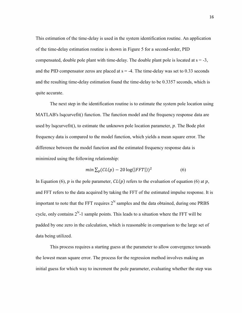
The next step in the identification routine is to estimate the system pole location using

MATLAB's lsqcurvefit() function. The function model and the frequency response data are

used by lsqcurvefit(), to estimate the unknown pole location parameter, . The Bode plot

frequency data is compared to the model function, which yields a mean square error. The

difference between the model function and the estimated frequency response data is

minimized using the following relationship:

(6)

In Equation (6), is the pole parameter, refers to the evaluation of equation (6) at ,

and FFT refers to the data acquired by taking the FFT of the estimated impulse response. It is

important to note that the FFT requires 2N samples and the data obtained, during one PRBS

cycle, only contains 2N-1 sample points. This leads to a situation where the FFT will be

padded by one zero in the calculation, which is reasonable in comparison to the large set of

data being utilized.

This process requires a starting guess at the parameter to allow convergence towards

the lowest mean square error. The process for the regression method involves making an

initial guess for which way to increment the pole parameter, evaluating whether the step was

17

in a direction that reduces the mean square error, and deciding which way to step next to

continue to cause a decrease in mean square error. This is referred to as the gradient descent

method and is discussed in Isermann and Münchhof's text (2011). This process is repeated

until the change in mean square error between iterations reaches a specific tolerance value or

the number of function evaluations exceeds a pre-set limit. This is to ensure the function

times out in a situation where the result does not converge.

If the initial guess for the system uses a large pole parameter value, there is still a

chance that the routine will not find the actual pole location. There is also a local minimum

other than the global minimum for the error. This local minimum occurs at a parameter value

of zero as can be seen in Figure 6.

Figure 6 exhibits the behavior of the mean square error for a large range of pole

parameters. In this case, the system was of second-order with time-delay and the double plant

poles were located at s = -15, which is seen as the global mean square error minimum. If the

algorithm took too large of a step as it approached the global minimum, it may have found

the local minimum at s = 0 instead. This problem is alleviated by the algorithm adjusting step

size based on the change in mean square error between iterations. This ensures that the initial

steps are large and the steps near the solution become smaller to converge quickly to a

solution and prevent missing of the global minimum. See Appendix B for the MATLAB

code used in the identification routine.

18

Figure 6 - Mean Square Error vs. Pole Parameter for a Second-Order System With Time-

Delay

Example mean square error curve for identifying a second-order system with system poles at s = -15. This curve

shows that the mean square error continues to rise as the estimated plant pole is evaluated at higher frequencies.

The graph also shows that there is a global minimum at the identified pole where s = -15 and a local minimum

at s = 0. A large initial guess for the system pole is a good starting point since the gradient descent technique

will likely find the global minimum.

2.3 Compensator Tuning for the First-Order Plant With Time-Delay

Once a transfer function model has been determined, the closed-loop poles must be

placed to achieve the desired overshoot. This concept was explored by Baker (2011) for

time-delay values that fall into a reasonable class. In this class, the closed-loop poles can be

moved far enough into the left hand plane to produce an accelerated system response. For

0 20 40 60 80 100 120

200

400

600

800

1000

1200

1400

X: 15

Y: 334.5

Parameter Input (rad/s)

Mea

n S

qu

are

Err

or

Mean Square Error for Paramter Variation

19

values outside this range, the time-delay effects on the system adversely affect the Root

Locus, causing an inability to move the closed-loop poles far enough to the left to achieve a

faster system response.

The development of this method requires the defining of a ratio known as normalized

time-delay (NTD) which is the ratio of the time-delay inherent in the system, Td, versus the

time constant of the open loop plant pole T (Astrom & Hagglund, 1995). This relationship is

shown in the following equation:

(7)

The range of NTD that Baker's method (2011) analyzed included NTD of 0.05 to 0.5. The

real-time auto tuning algorithm accommodates the same range of NTD, as discussed in

Baker's method, but extends the idea to larger values of NTD. In these cases, the closed-loop

poles will not be able to be placed far enough into the left half plane to accelerate the system

response, as shown in Figure 7 for an NTD of 1. However, the system will still be tunable to

achieve a desired overshoot, by sacrificing the response time.

Due to the nature of the time-delayed system, traditional Root Locus methods cannot

be applied unless time-delay poles are accounted for. These pole loci run roughly parallel to

the real axis, and occur with spacing of

radians due to the effects of the complex

exponential. For NTD values greater than 0.5, the pole loci begin to come close enough to

the plant poles to have a drastic effect on the Root Loci, as shown in Figure 7. In many cases,

the compensator zeros that are added into the system will no longer attract the plant poles.

The compensator zeros will now attract the poles created by the time-delay. This leaves the

plant poles to be driven into the right half plane causing instability for even moderate gain

20

values. This behavior is shown for an example first-order system, with time-delay of 0.25

seconds and NTD = 1. In this case, the closed-loop plant poles migrate to instability at a gain

of approximately 5.2. In this case, the PI compensator added will not accomplish the goal of

a faster response for the system since there is no way to move the closed-loop plant poles

further into the left half plane.

Figure 7 - Root Locus for First-Order PI Compensated Plant With

Normalized Time-Delay = 1

Generated Using Time-Delay Exponential (Baker, 2011)

Root Locus plot showing behavior of a first-order plant with a plant pole at s = -4 and a compensator zero

placed at s = -5. This figure shows that the closed-loop plant poles are no longer able to be drawn to the left by

the compensator zero. Instead, they migrate into the right half plane and exhibit marginal stability at a gain of

5.2. The figure also shows the time-delay poles separated by

= 25.12. The time-delay poles have been

repelled by the plant poles to a value of approximately 30.

-10 -8 -6 -4 -2 0 2-40

-30

-20

-10

0

10

20

30

40

X: -0.05

Y: -5.7

Z: 5.2

Real Axis

Ima

gin

ary

Axis

Root Locus

Root Locus

Open Loop Pole

Open Loop Zero

Gain0

1

2

3

4

5

6

7

8

9

10

21

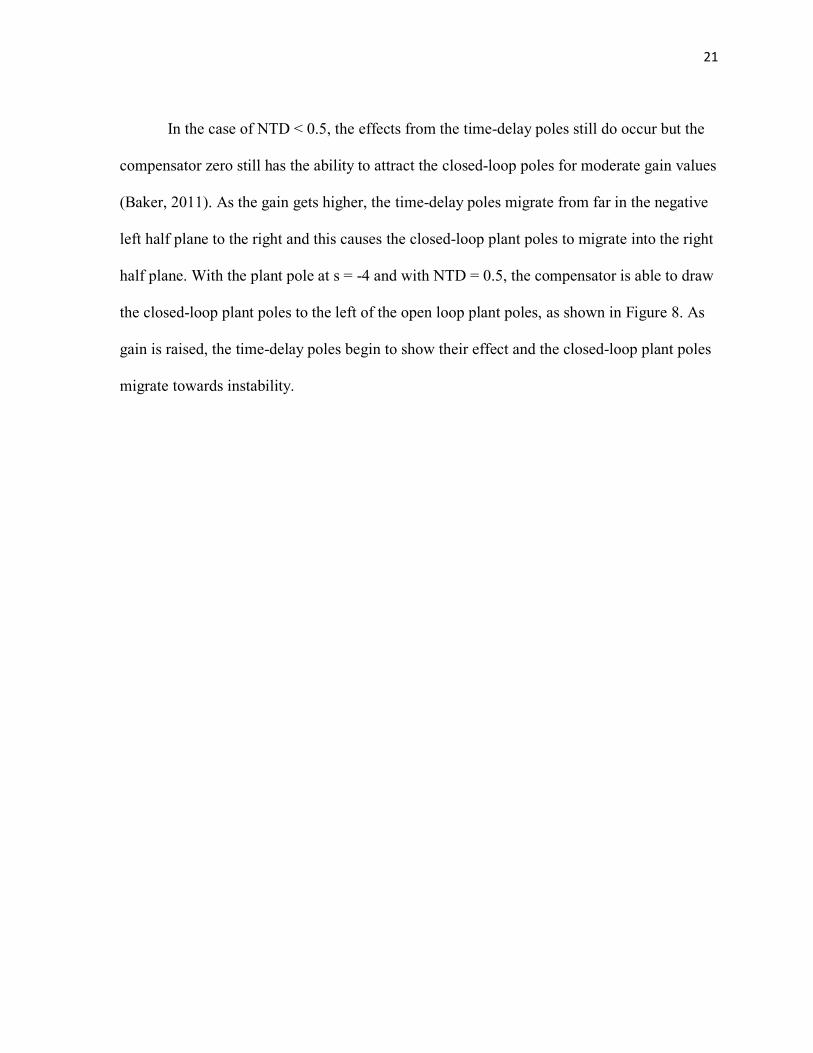
In the case of NTD < 0.5, the effects from the time-delay poles still do occur but the

compensator zero still has the ability to attract the closed-loop poles for moderate gain values

(Baker, 2011). As the gain gets higher, the time-delay poles migrate from far in the negative

left half plane to the right and this causes the closed-loop plant poles to migrate into the right

half plane. With the plant pole at s = -4 and with NTD = 0.5, the compensator is able to draw

the closed-loop plant poles to the left of the open loop plant poles, as shown in Figure 8. As

gain is raised, the time-delay poles begin to show their effect and the closed-loop plant poles

migrate towards instability.

22

Figure 8 - Root Locus for a First-Order PI Compensated Plant, With

Normalized Time-Delay = 0.5, Showing Closed-loop Poles Being Drawn to the Left,

Generated Using Time-Delay Exponential (Baker, 2011)

Root Locus plot showing the closed-loop poles being drawn further into the left half plane, which will make the

system response quicker. This will also cause the system to ring due to the complex conjugate poles. Baker's

method (2011) utilized this approach to draw the poles further into the left half plane and then reduced the gain

to balance the overshoot and load disturbance rejection. The real-time auto tuning algorithm focuses on

targeting a commanded overshoot. The plant pole for this system is located at s = -4 and the compensator zero is

located at s = -5. The saddle point of the loci occurs at a gain of 4 and this gain places the dominant closed-loop

poles at s = -4.6 ± 5.4j.

Utilizing Baker's approach (2011) to tune the system for quick response and

overshoot reduction, a PI compensator zero is placed at 1.5 times the plant pole for an NTD

of 0.5. This places the zero at s = -6 with a recommended loop gain of 1 to achieve the

response shown in Figure 9.

-10 -9 -8 -7 -6 -5 -4 -3 -2 -1 0-15

-10

-5

0

5

10

15

X: -4.6

Y: 5.4

Z: 4

Real Axis

Ima

gin

ary

Axis

Root Locus

Root Locus

Open Loop Pole

Open Loop Zero

Gain0

1

2

3

4

5

6

7

8

9

10

23

Figure 9 - Root Locus Plot for First-Order PI Compensated Plant, With

Normalized Time-Delay = 0.5, Utilizing the Compensator Placement Method from Baker's

Approach (2011), Generated Using Time-Delay Exponential

Root locus demonstrating the compensator zero placement using Baker's method (2011). This method involves

the placement of the zero at 1.5 times the plant pole which is located at s = -4, for an NTD of 0.5. This places

the compensator zero at s = -6. In this case, the closed-loop plant poles are not drawn very far into the left half

plane which leads to a result that is not optimum for time response performance. In this compensator placement,

the saddle point places the closed-loop poles at s = -3.35 ± 5.75j which does not provide a performance increase

over the open loop plant poles. This system has an inherent time-delay of 0.125 seconds.

An important note for this Root Locus is that the closed-loop poles for this plant are

stable with relatively low overshoot and no steady state error. However, even by properly

adjusting the gain to the saddle of the loci, as shown in the figure for a loop gain of 4, the

closed-loop poles of the system will not provide a faster response than the open loop poles of

-10 -9 -8 -7 -6 -5 -4 -3 -2 -1 0-15

-10

-5

0

5

10

15

X: -3.35

Y: 5.75

Z: 4

Real Axis

Ima

gin

ary

Axis

Root Locus

Root Locus

Open Loop Pole

Open Loop Zero

Gain0

1

2

3

4

5

6

7

8

9

10

24

the system. At a gain of 4, the closed-loop poles are drawn as far as possible into the left half

plane and reach a value of s = -3.35 ± 5.75j. If the goal of adding a PI compensator is merely

system stability and setpoint tracking, this would be an adequate solution. However, in many

cases, performance is one of the most important factors in the design.

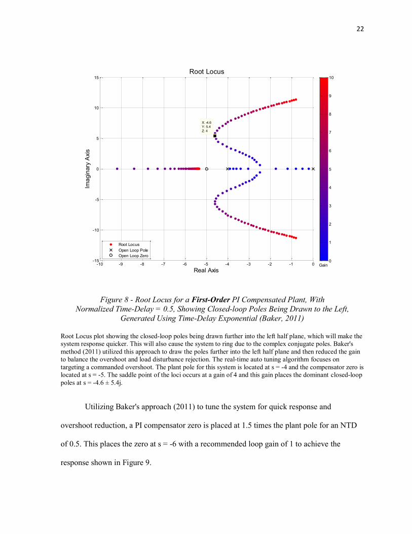
In order to adjust the system closed-loop poles to achieve a desired overshoot and

ensure an adequate performance gain with no steady state error, the compensator PI zero

must be moved closer to the open loop plant pole. This allows for a greater attraction

between the pole and zero and allows for a larger draw of the closed-loop poles into the left

half plane, before being affected by the time-delay poles. To keep a reasonable separation of

the compensator zero and pole, the compensator zero will be placed at 1.1 times the plant

pole. This consistent pole placement for various NTD values will allow more opportunity for

the Root Loci to be drawn to the left, allowing for a faster system response. The Root Locus

that exemplifies this pole placement scenario is shown in Figure 10, which shows a large

performance gain over the Baker method (2011). Because of this performance gain, this is

the method of compensator zero placement that will be applied in the real-time auto tuning

algorithm. This system has a plant pole at s = -4 and a compensator zero placed at s = -4.4,

with a time-delay of 0.125 seconds.

25

Figure 10 - Root Locus Plot for a First-Order PI Compensated System With

Normalized Time-Delay = 0.5, Showing Higher Performance

Generated Using Time-Delay Exponential (Baker,2011)

This figure shows the modified pole placement method that demonstrates the capability of providing higher

performance in a first-order PI compensated system. The plant pole is located at s = -4 and, by placing the pole

at 1.1 times the location of the open loop pole, the Root Locus is drawn further to the left. This compensator

zero placement shows a marked performance increase over the results shown in Figure 9, with the closed-loop

plant poles being drawn to s = -6.05 ± 4.3j at a gain of 3.6. The point selected on the Loci in the figure shows

the fastest system response achievable with this system for an NTD of 0.5.

-9 -8 -7 -6 -5 -4 -3 -2 -1 0-15

-10

-5

0

5

10

15

X: -6.05

Y: 4.3

Z: 3.6

Real Axis

Ima

gin

ary

Axis

Root Locus

Root Locus

Open Loop Pole

Open Loop Zero

Gain0

1

2

3

4

5

6

7

8

9

10

26

2.4 Compensator Tuning for the Second-Order Plant With Time-Delay

This research focused on the compensation of a double pole plant. In a second-order

PID compensated plant, the closed-loop poles are moved further into the left half plane by

the compensator double zero placement. This case is similar to the first-order case but the

maximum acceleration of the plant response will also be dictated by the closed-loop pole that

travels from the double pole position towards the compensator zero along the real axis. One

of the closed-loop plant poles migrates in each direction along the real axis. The pole

migrating to the left, approaches one of the compensator zeros and the other moves to the

right, where it collides with the integrator pole. The two closed-loop poles then break away

from the real axis. The closed-loop poles are forced into the right half plane for higher gains

due to influence from the time-delay poles. There is also a time-delay pole that migrates from

negative infinity towards the second compensator zero for higher gains.

Just as in the single pole plant case, there will be an attempt to apply the Baker

method (2011) to accomplish adequate tuning of the system, by moving the closed-loop

plant poles as far to the left as possible. The Baker method recommends placing the double

compensator zeros at 1.06 times the double pole position. This will be at s = -3.18. This

corresponds to PID compensator values of kd = 1, kp = 6.36, and ki = 10.1124. In this case,

the Baker method recommends a gain of 1.7. The optimum acceleration of the plant response

would occur at the saddle point of the graph which occurs at a loop gain of 2.8, as shown in

Figure 11.

27

Figure 11 - Root Locus Plot for Second-Order PID Compensated Plant With

Normalized Time-Delay = 0.5 and Compensator Zero Placement Utilizing Baker Method

(2011) Generated Using Time-Delay Exponential

Root Locus plot showing the application of Baker's method (2011) for a second-order PID compensated plant

with NTD of 0.5. In this case, the optimum plant response acceleration occurs at a gain of 2.8, while Baker's

method recommends a gain of 1.7, for overshoot reduction and disturbance rejection. The plant involves a

double pole at s = -3 and a double compensator zero placed at s = -3.18. The time-delay for this system is 0.167

seconds.

In the case of the second-order plant, the Baker method (2011) provides an ample

double compensator zero placement to move the closed-loop poles further into the left half

plane. However, the gain adjustment needs to be modified to allow for a balance between

-10 -8 -6 -4 -2 0 2-10

-8

-6

-4

-2

0

2

4

6

8

10

X: -2.4

Y: 1.2

Z: 1.6

Real Axis

Ima

gin

ary

Axis

Root Locus

X: -4.3

Y: 3.55

Z: 2.8

Root Locus

Open Loop Pole

Open Loop Zero

Gain0

1

2

3

4

5

6

7

8

9

10

28

system response and overshoot. To apply a consistent method, as in the single pole plant

case, it is important to keep the ratio of the double plant pole location to the PID compensator

zeros constant. This allows for predictable behavior over a larger range of NTD values. After

experimenting with compensator zero placement locations, it was noticed that the

compensator zeros can more aggressively compensate the system when placed on either side

of the double plant pole for large values of NTD. The compensator zero locations were

chosen as 1.1 and 0.9 times the double plant pole location. This compensator placement leads

to a scenario where the integrator pole is attracted to the compensator zero, to the right of the

double plant poles, the time-delay zero comes from negative infinity and is attracted towards

the zero to the left of the plant poles, and the two plant poles break away immediately from

the real axis to be driven to the right by the time-delay poles. This allows for a best case

closed-loop performance that occurs at the open loop zero location to the right of the plant

poles, as shown in Figure 12. This does not create much of a performance increase over the

Baker approach (2011) for ranges of NTD between 0.05 and 0.5, but allows for better tuning

when the time-delay is on the order of the plant time constant.

For large NTD, this compensator zero placement method provides a notable

performance increase over the Baker method (2011). Take for example the same plant with

an NTD of 2. Utilizing the pole placement method applied by Baker yields the best case

closed-loop performance at a double plant pole of s = -1.15. This is 38% of the performance

of the open loop poles. By applying the pole placement method used in the algorithm, the

best case plant pole placement for performance occurs at s = -1.85. This is 61.7% of the open

loop plant time constant so this method will be utilized in the development of the auto tuning

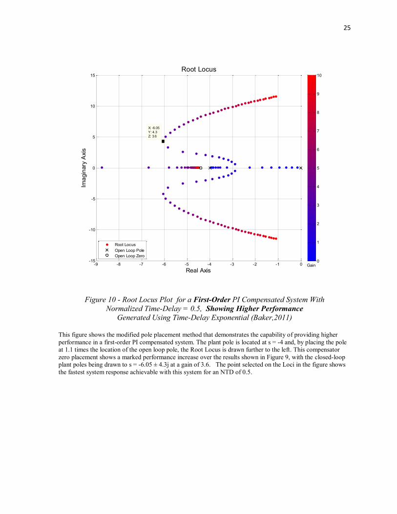
29

algorithm. This Root Locus behavior is shown in Figure 13 for the Baker method (2011) and

Figure 14 for the method used in the algorithm. It is important to note that the Baker method

was not developed for NTD greater than 0.5 and the result is only included for comparison.

Figure 12 -Root Locus for a Second-Order PID Compensated System With

Normalized Time-Delay = 0.5 Utilizing the Algorithm Approach


This Root Locus plot shows that the compensator zero placement, at 0.9 and 1.1 times the plant poles, applied

in the algorithm does not show performance gains over Baker's method (2011) for NTD on the order of 0.5. The

figure does show that there is a much larger draw of the closed-loop poles into the left half plane which is

leveraged for NTD values greater than 0.5. In the case of this plant, with compensator zeros placed at s = -3.3,

-2.7, the response of the system is still limited by the migration of the integrator pole.

-10 -8 -6 -4 -2 0 2-10

-8

-6

-4

-2

0

2

4

6

8

10

Real Axis

Ima

gin

ary

Axis

Root Locus

Root Locus

Open Loop Pole

Open Loop Zero

Gain0

1

2

3

4

5

6

7

8

9

10

30

Figure 13 - Root Locus for a Second-Order PID Compensated System With

Normalized Time-Delay = 2 Utilizing the Baker Method (2011) for Normalized Time-Delay

= 0.5 Generated Using Time-Delay Exponential

Root Locus plot showing the performance of Baker's compensator zero placement method (2011) for the double

pole system with s = -3. In this case the compensator double zero is placed at s = -3.18 which is 1.06 times the

double plant pole. The fastest system response is achievable at the break away point where the closed-loop plant

poles are located at s = -1.15, which is 38% of the open loop plant pole time constant. It is important to note that

Baker's method does not cover NTD in this region, but the result is shown for comparison.

-5 -4 -3 -2 -1 0 1-15

-10

-5

0

5

10

15

X: -1.15

Y: 0.1

Z: 0.4

Real Axis

Ima

gin

ary

Axis

Root Locus

Root Locus

Open Loop Pole

Open Loop Zero

Gain0

0.2

0.4

0.6

0.8

1

1.2

1.4

1.6

1.8

2

31

Figure 14 - Root Locus for a Second-Order PID Compensated System With

Normalized Time-Delay = 2 Utilizing the Algorithm Method


This Root Locus shows the performance gain using the new compensator placement technique. The plant is still

a double pole plant with s = -3, but the compensator zeros are placed on either side of the plant poles at 1.1 and

0.9 times the double pole location. This causes the plant poles to immediately break away from the real axis

which causes higher performance to be achieved, before the closed-loop poles migrate to the right. This is a

large improvement over Baker's method (2011), which produced closed-loop plant poles at s = -1.15. This

method produced closed-loop plant poles at s = -1.85 ± 0.25j.

2.5 Real-Time Gain Calculation for Systems With Time-Delay

The next portion of the compensator adjustment relies on the automatic determination

of gain to achieve the proper overshoot. This portion of the algorithm relies on a close

estimate of the plant pole location to ensure that the compensator zero is placed at the

32

appropriate location for the Root Locus to be predictable. If there is error in the identified

pole location, or in the estimation of the system time-delay, the gains calculated by this

method will not be as accurate as desired.

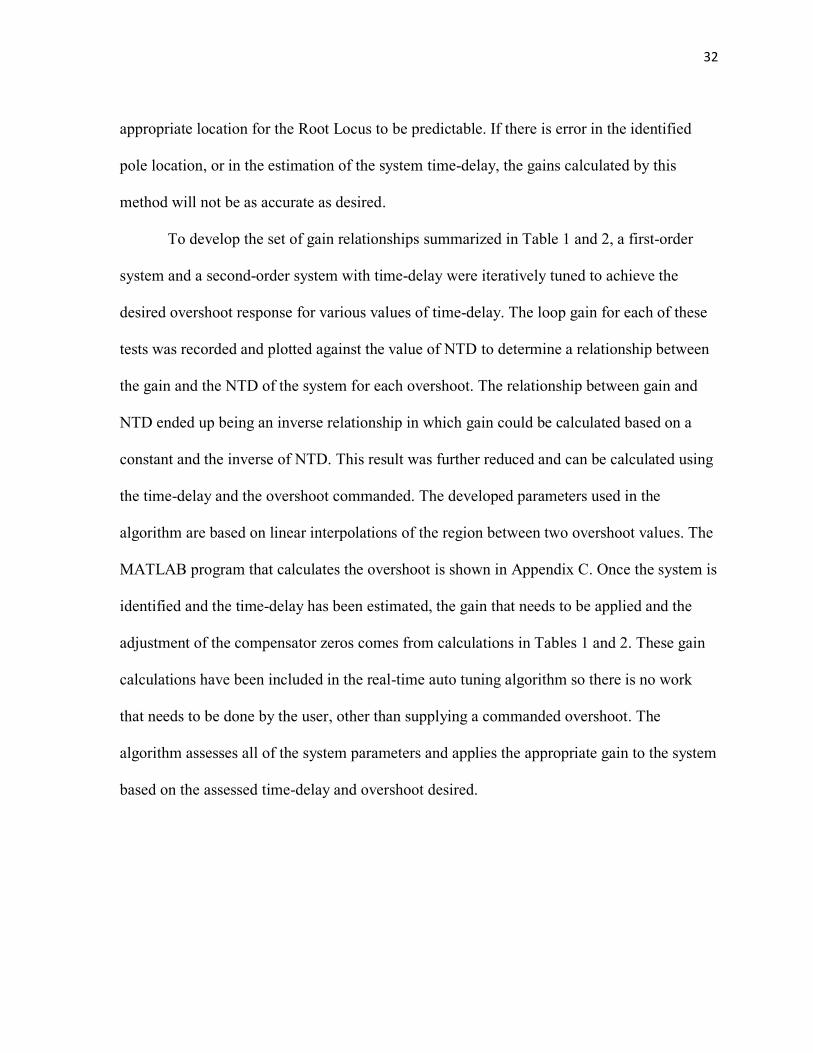
To develop the set of gain relationships summarized in Table 1 and 2, a first-order

system and a second-order system with time-delay were iteratively tuned to achieve the

desired overshoot response for various values of time-delay. The loop gain for each of these

tests was recorded and plotted against the value of NTD to determine a relationship between

the gain and the NTD of the system for each overshoot. The relationship between gain and

NTD ended up being an inverse relationship in which gain could be calculated based on a

constant and the inverse of NTD. This result was further reduced and can be calculated using

the time-delay and the overshoot commanded. The developed parameters used in the

algorithm are based on linear interpolations of the region between two overshoot values. The

MATLAB program that calculates the overshoot is shown in Appendix C. Once the system is

identified and the time-delay has been estimated, the gain that needs to be applied and the

adjustment of the compensator zeros comes from calculations in Tables 1 and 2. These gain

calculations have been included in the real-time auto tuning algorithm so there is no work

that needs to be done by the user, other than supplying a commanded overshoot. The

algorithm assesses all of the system parameters and applies the appropriate gain to the system

based on the assessed time-delay and overshoot desired.

33

Table 1

Recommended PI Tuning Relationships for a First-Order Plant With Time-Delay

Overshoot (%) Gain

0-4

4-10

10-20

20-30

Greater than 30

This table provides recommended gain calculations for a first-order PI compensated system, based on overshoot

and time-delay inherent in the system, utilizing a compensator zero placement at 1.1 times the plant pole.

34

Table 2

Recommended PID Tuning Relationships for a Second-Order Plant With Time-Delay

Overshoot (%) Gain

0-4

4-10

10-20

20-30

Greater than 30

This table shows recommended gain calculations, utilizing a commanded overshoot and a system time-delay,

for a second-order PID compensated plant with zero placements at 1.1 times the double plant pole and 0.9 times

the double plant pole location.

It is desirable to be able to choose a tradeoff between overshoot and time response, so

the algorithm was developed to accommodate an automatic choice of gain based on the

desired overshoot. The idea behind this approach is that a user can specify the overshoot that

the system can support and the best response gain will be chosen for the current plant, the

compensated PID, and the current system time-delay. To illustrate the performance of the

method for a first-order PI compensated system, Figures 14 and 15 show the step responses

for various selected overshoots in specific NTD situations. As one can see from the figures,

the results are fairly consistent over a range of NTD. By improving this relationship and

35

finding a function to describe the relationship between overshoot, NTD, and tuned gain, the

responses could be idealized to match perfectly in all scenarios. As the algorithm stands

today, the responses are not ideal due to linear interpolations utilized in the development of

the algorithm. One important aspect of this approach is that the computation requirement is

much lower than an analytical solution and is feasible with simple mathematical operations.

One important aspect of this approach is that there is no accelerating of the system

response for larger values of NTD. However, the plant response matches the expected value

of overshoot while maximizing the performance, for this compensator placement method. In

the case of large NTD, the time-delay poles push the system towards instability. With a

traditional PI or PID compensator, the best that can be accomplished is to stabilize the system

and make a compromise for overshoot if time performance is required.

Utilizing the iterative tuning approach, a set of equations was also developed for a

second-order PID compensated system. In this case, the poles are placed on either side of the

plant poles offset by ±10% of the open loop plant pole value. Assuming this pole placement,

a gain calculation is performed which will yield the appropriate overshoot for the given

NTD. An example of the step responses for various requested overshoots and NTD values is

shown in Figures 17 and 18, for a second-order plant. Note that this set of responses was

much easier to perform linear interpolation for the data due to the symmetric nature of the

zero placement. It does not exhibit the same issues as the method applied to the first-order

plant.

36

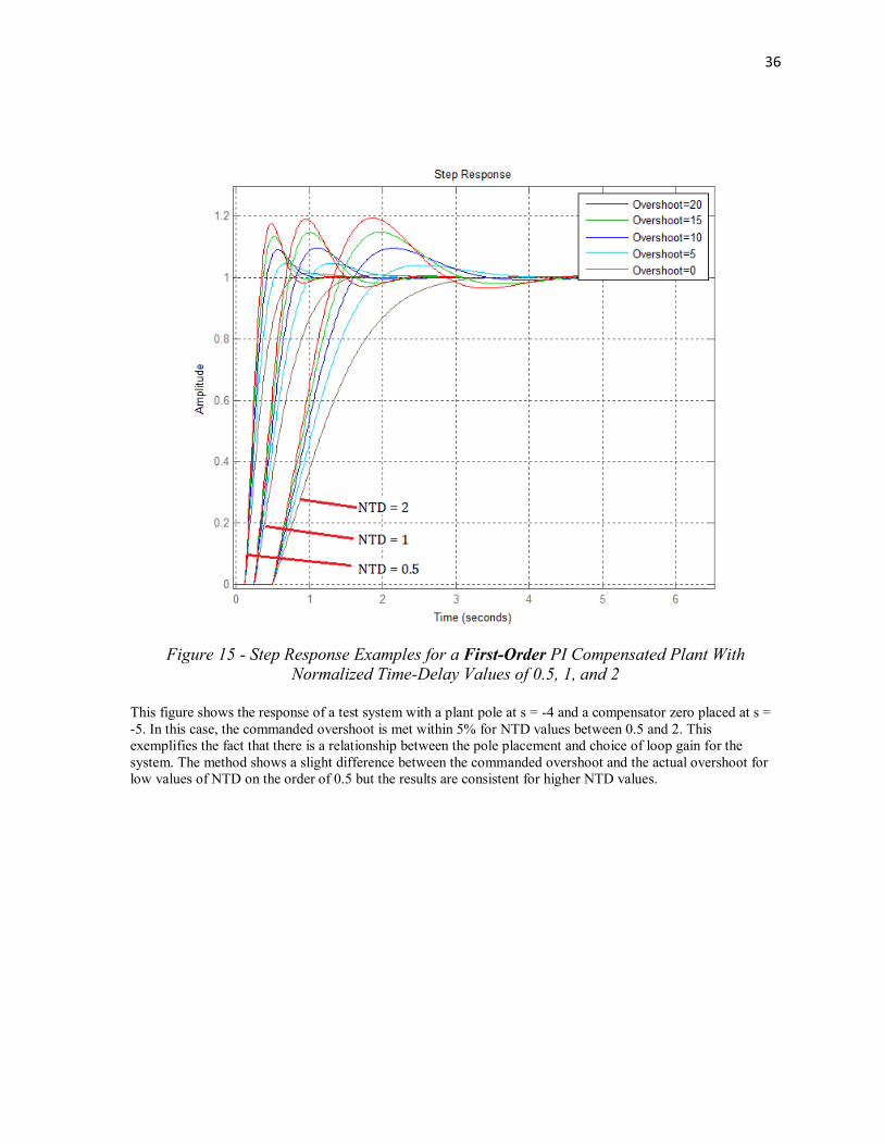
Figure 15 - Step Response Examples for a First-Order PI Compensated Plant With Normalized Time-Delay Values of 0.5, 1, and 2

This figure shows the response of a test system with a plant pole at s = -4 and a compensator zero placed at s =

-5. In this case, the commanded overshoot is met within 5% for NTD values between 0.5 and 2. This

exemplifies the fact that there is a relationship between the pole placement and choice of loop gain for the

system. The method shows a slight difference between the commanded overshoot and the actual overshoot for

low values of NTD on the order of 0.5 but the results are consistent for higher NTD values.

37

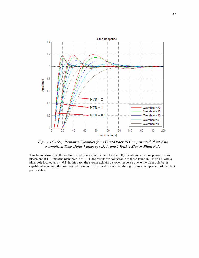
Figure 16 - Step Response Examples for a First-Order PI Compensated Plant With

Normalized Time-Delay Values of 0.5, 1, and 2 With a Slower Plant Pole

This figure shows that the method is independent of the pole location. By maintaining the compensator zero

placement at 1.1 times the plant pole, s = -0.11, the results are comparable to those found in Figure 15, with a

plant pole located at s = -0.1. In this case, the system exhibits a slower response due to the plant pole but is

capable of achieving the commanded overshoot. This result shows that the algorithm is independent of the plant

pole location.

38

Figure 17 - Step Response Examples for a Second-Order PID Compensated Plant With

Normalized Time-Delay Values of 0.5, 1, and 2

This figure illustrates that compensator zero placements of 1.1 and 0.9 times the open loop plant pole location,

s = -3, yield satisfactory overshoot responses for NTD from 0.5 to 2. In this case, commanded overshoot

matches the ideal overshoot perfectly.

39

Figure 18 - Step Response Examples for a Second-Order PID Compensated Plant With

Normalized Time-Delay Values of 0.5, 1, and 2 With a Slower Double Plant Pole

This figure is used to exemplify that the method is independent of pole location and shows comparable results

with respect to the last example. In this case, the NTD is varied between 0.5 and 2 and the double plant pole has

been relocated to s = -0.1. The system response is much slower due to the double plant pole location.

40

3. Validation of the Cross-Correlation and System Identification Portions of the Real-

Time Auto Tuning Algorithm

This chapter is devoted to the validation of the auto-tuning algorithm by comparing

the output of the algorithm to known classical results. The algorithm involves steps that can

be generalized to plants that do not exhibit time-delay, including the injection of the PRBS

and the identification of the system's closed-loop plant poles. The algorithm is validated on a

first-order PI compensated plant and a second-order PID compensated plant, with time-delay

set to zero.

3.1 First-Order PI Compensated Plant With Zero Time-Delay

The first-order PI compensated plant is shown in Figure 19. The remainder of the

algorithm blocks including PRBS injection, cross correlation of input and output to estimate

the impulse response, and the identification of the system have not been included in this

figure but are shown in Figure 3.

Figure 19 - First-Order PI Compensated System With Zero Time-Delay

This figure shows the first-order plant utilized for the validation of the algorithm. This plant does not have time-

delay so the algorithm is applied with time-delay set to zero. The plant is a single pole plant with plant pole at p,

proportional gain kp, and integral gain ki. The algorithm portions of the system are not shown but include PRBS

injection, cross correlation of input and output, and system identification, as shown in Figure 3.

41

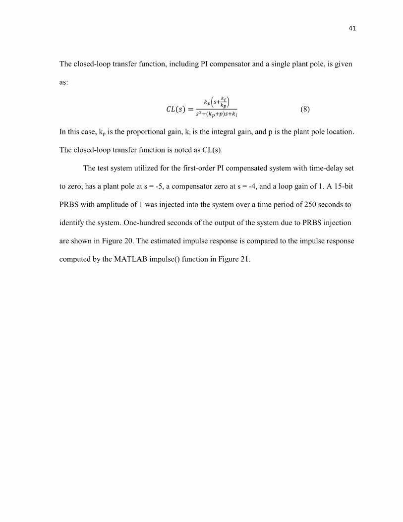
The closed-loop transfer function, including PI compensator and a single plant pole, is given

as:

(8)

In this case, kp is the proportional gain, ki is the integral gain, and p is the plant pole location.

The closed-loop transfer function is noted as CL(s).

The test system utilized for the first-order PI compensated system with time-delay set

to zero, has a plant pole at s = -5, a compensator zero at s = -4, and a loop gain of 1. A 15-bit

PRBS with amplitude of 1 was injected into the system over a time period of 250 seconds to

identify the system. One-hundred seconds of the output of the system due to PRBS injection

are shown in Figure 20. The estimated impulse response is compared to the impulse response

computed by the MATLAB impulse() function in Figure 21.

42

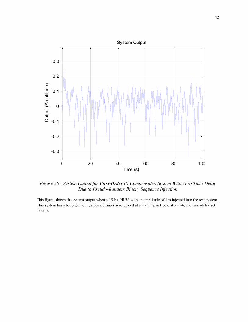
Figure 20 - System Output for First-Order PI Compensated System With Zero Time-Delay

Due to Pseudo-Random Binary Sequence Injection

This figure shows the system output when a 15-bit PRBS with an amplitude of 1 is injected into the test system.

This system has a loop gain of 1, a compensator zero placed at s = -5, a plant pole at s = -4, and time-delay set

to zero.

0 20 40 60 80 100

-0.3

-0.2

-0.1

0

0.1

0.2

0.3

Time (s)

Outp

ut

(Am

plitu

de

)System Output

43

Figure 21 - Impulse Response Comparison between MATLAB impulse() Function (blue) and

Cross-Correlation Result (red) of a First-Order PI Compensated System With Zero Time-

Delay

This figure shows the estimated impulse response from the cross correlation output in red, compared to the

impulse response from the MATLAB impulse() function in blue. This system has a loop gain of 1, a

compensator zero placed at s = -5, a plant pole at s = -4, and time-delay set to zero.

The system identification routine identified the open loop plant pole at s = -3.8082

with the actual plant pole being located at s = -4. This validates the use of PRBS injection,

cross correlation of input and output to obtain the impulse response estimate, and the proper

identification of the system using the MATLAB lsqcurevefit() function, for a first-order

0 0.5 1 1.5 2 2.5 3 3.5 4 4.5 50

0.1

0.2

0.3

0.4

0.5

0.6

0.7

0.8

0.9

1Impulse Response

Time (seconds)

Am

plit

ud

e

44

system with time-delay set to zero. The Bode plot of the frequency response is shown in

Figure 22.

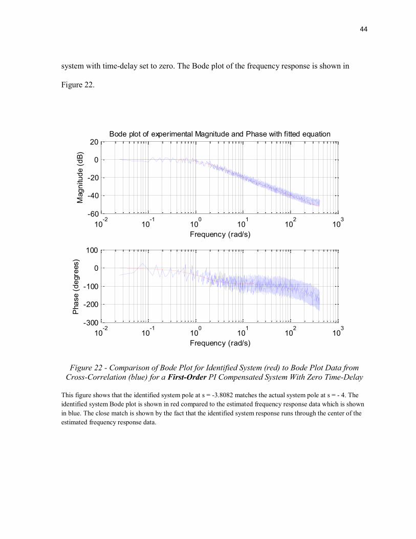
Figure 22 - Comparison of Bode Plot for Identified System (red) to Bode Plot Data from

Cross-Correlation (blue) for a First-Order PI Compensated System With Zero Time-Delay

This figure shows that the identified system pole at s = -3.8082 matches the actual system pole at s = - 4. The

identified system Bode plot is shown in red compared to the estimated frequency response data which is shown

in blue. The close match is shown by the fact that the identified system response runs through the center of the

estimated frequency response data.

10-2

10-1

100

101

102

103

-60

-40

-20

0

20

Mag

nitu

de (

dB

)

Frequency (rad/s)

Bode plot of experimental Magnitude and Phase with fitted equation

10-2

10-1

100

101

102

103

-300

-200

-100

0

100

Pha

se (

de

gre

es)

Frequency (rad/s)

45

3.2 Second-Order PID Compensated Plant With Zero Time-Delay

The second-order PID compensated plant is shown in Figure 23. The remainder of the

algorithm blocks including PRBS injection, cross correlation of input and output to obtain the

impulse response estimate, and the system identification blocks have not been included in

this figure but are shown in Figure 3. The plant is given in the general form but the system

tested in this analysis involves a second-order plant with a double pole.

Figure 23- Second-Order PID Compensated System With Zero Time-Delay

This figure shows the second-order plant utilized for the validation of the algorithm. This plant does not have

time-delay so the algorithm is applied with time-delay set to zero. The plant is a double pole plant with plant

poles at p, a derivative gain kd, proportional gain kp, and integral gain ki. The algorithm portions of the system

are not shown but include PRBS injection, cross correlation of the input and output to obtain the impulse

response estimate, and system identification, as shown in Figure 3.

The plant is a double pole plant with poles placed at p, the closed-loop transfer

function, including PID compensator and a double plant pole, takes the following form:

(9)

In this case, kd is the derivative gain, kp is the proportional gain, ki is the integral gain, and p

is the double plant pole location. The closed-loop transfer function is noted as CL(s).

46

The test system utilized for this validation has a double plant pole at s = -3, a double

compensator zero at s = -15, and a loop gain of 1. A 15-bit PRBS with amplitude of 1 was

injected into the system over a time period of 250 seconds to identify the system. One-

hundred seconds of the output of the system, due to PRBS injection, is shown in Figure 24.

The estimated impulse response is compared to the MATLAB impulse() function and is

shown in Figure 25.

Figure 24 - System Output for Second-Order PID Compensated System With Zero Time-

Delay Due to Pseudo-Random Binary Sequence Injection

This figure shows the system output when a 15-bit PRBS with an amplitude of 1 is injected into the test system.

This system has a loop gain of 1, a double compensator zero placed at s = -15, a double plant pole at s = -3, and

time-delay set to zero.

0 20 40 60 80 100

-1

-0.5

0

0.5

1

Time (s)

Outp

ut

(Am

plitu

de

)

System Output

47

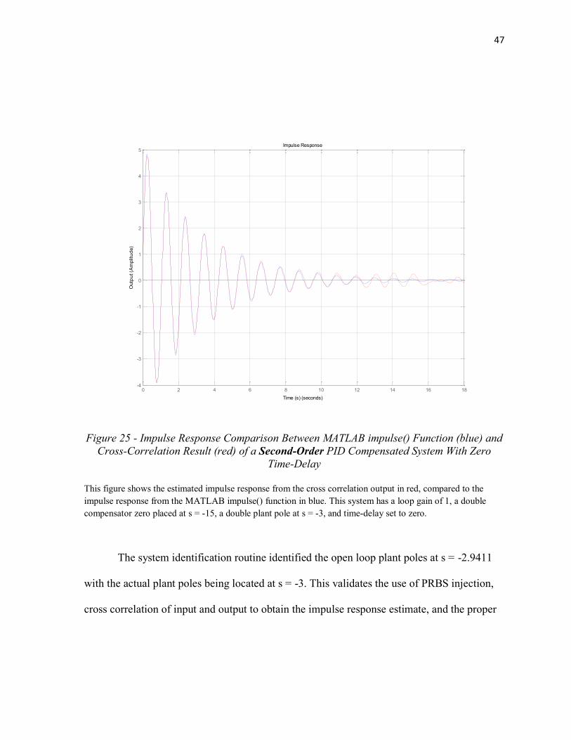
Figure 25 - Impulse Response Comparison Between MATLAB impulse() Function (blue) and

Cross-Correlation Result (red) of a Second-Order PID Compensated System With Zero

Time-Delay

This figure shows the estimated impulse response from the cross correlation output in red, compared to the

impulse response from the MATLAB impulse() function in blue. This system has a loop gain of 1, a double

compensator zero placed at s = -15, a double plant pole at s = -3, and time-delay set to zero.

The system identification routine identified the open loop plant poles at s = -2.9411

with the actual plant poles being located at s = -3. This validates the use of PRBS injection,

cross correlation of input and output to obtain the impulse response estimate, and the proper

0 2 4 6 8 10 12 14 16 18-4

-3

-2

-1

0

1

2

3

4

5Impulse Response

Time (s) (seconds)

Outp

ut (A

mplit

ud

e)

48

identification of the system using the MATLAB lsqcurevefit() function for a second-order

system with no time-delay. The Bode plot of the frequency response is shown in Figure 26.


Cross-Correlation (blue) of a Second-Order PID Compensated System With Zero Time-

Delay

This figure shows that the identified double plant poles at s = -2.9411 match the actual double plant poles at s =

-3. The identified system Bode plot is shown in red compared to the estimated frequency response data which is

shown in blue. The close match is shown by the fact that the identified system response runs through the center

of the estimated frequency response data.

10-2

10-1

100

101

102

103

-60

-40

-20

0

20

40

Mag

nitu

de (

dB

)

Frequency (rad/s)


10-2

10-1

100

101

102

103

-250

-200

-150

-100

-50

0

50

Pha

se (

de

gre

es)

Frequency (rad/s)

49

These data validate the algorithm for first and second-order systems with time-delay

set to zero. A PRBS was injected into the system, the cross correlation of the input and

output was performed, and the system was identified in both the first and second-order cases.

50

4. Results of Real-Time Auto Tuning Algorithm on Plants With Time-Delay

This chapter focuses on the results of the algorithm when run on systems in the NTD

region of 0.5 to 1. The algorithm is first demonstrated using an NTD of 0.5. This

demonstration is followed by an example of the algorithm's ability to properly tune a time-

delayed first and second-order system for NTD of 1.

4.1 First-Order PI Compensated Plant With Normalized Time-Delay = 0.5

The first-order PI compensated plant with time-delay is shown in Figure 27. The

remainder of the algorithm blocks including PRBS injection, cross correlation of input and

output to obtain the impulse response estimate, system identification, gain calculation, and

closed-loop pole placement have not been included in this figure but are shown in Figure 3.

Figure 27 - First-Order PI Compensated Plant With Time-Delay

The plant is a single pole plant with plant pole at p, proportional gain kp, integral gain ki. and time-delay Td. The

algorithm portions of the system are not shown but include PRBS injection, cross correlation of input and

output to obtain the impulse response estimate, system identification, and gain calculation, as shown in Figure

3.

51

The closed-loop transfer function of the system, including PI compensator, a single plant

pole, and internal time-delay, is given as:

(10)

In Equation (10) the time-delay is defined as Td, the plant pole is defined as p, the

proportional gain is kp, the integral gain is ki, and the closed-loop transfer function is given as

CL(s).

The test system utilized for this demonstration has a plant pole at s = -4, a

compensator zero at s = -5, a loop gain of 1, a time-delay of 0.125 seconds, and an NTD of

0.5. A 15-bit PRBS with an amplitude of 1 was injected into the system over a time period of

250 seconds to identify the system, assess the time-delay, place the compensator zeros and

adjust the loop gain to achieve the commanded overshoot. One-hundred seconds of the

output of the system due to PRBS injection is shown in Figure 28. The estimated impulse

response is shown in Figure 29.

52

Figure 28 - System Output for First-Order PI Compensated System With Time-Delay Due to Pseudo-Random Binary Sequence Injection

This figure shows 100 seconds of the system output when a 15-bit PRBS with an amplitude of 1 is injected into

the system. This system has a loop gain of 1, a compensator zero placed at s = -5, a plant pole at s = -4, and a

time-delay of 0.125 seconds. This delay corresponds to an NTD of 0.5, since the plant time constant is 0.25

seconds.

0 20 40 60 80 100

-0.3

-0.2

-0.1

0

0.1

0.2

0.3

Time (s)

Outp

ut

(Am

plitu

de

)

System Output

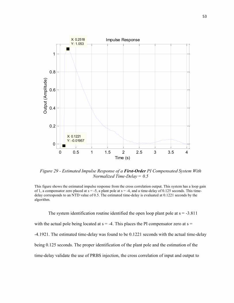
53

Figure 29 - Estimated Impulse Response of a First-Order PI Compensated System With

Normalized Time-Delay = 0.5

This figure shows the estimated impulse response from the cross correlation output. This system has a loop gain

of 1, a compensator zero placed at s = -5, a plant pole at s = -4, and a time-delay of 0.125 seconds. This time-

delay corresponds to an NTD value of 0.5. The estimated time-delay is evaluated at 0.1221 seconds by the

algorithm.

The system identification routine identified the open loop plant pole at s = -3.811

with the actual pole being located at s = -4. This places the PI compensator zero at s =

-4.1921. The estimated time-delay was found to be 0.1221 seconds with the actual time-delay

being 0.125 seconds. The proper identification of the plant pole and the estimation of the

time-delay validate the use of PRBS injection, the cross correlation of input and output to

0 0.5 1 1.5 2 2.5 3 3.5 4

0

0.2

0.4

0.6

0.8

1

X: 0.2518

Y: 1.053

X: 0.1221

Y: -0.01957

Time (s)

Outp

ut

(Am

plitu

de

)

Impulse Response

54

obtain the impulse response estimate, and the proper identification of the system using the

MATLAB lsqcurevefit() function. The Bode plot of the estimated frequency response is

shown in Figure 30.


Cross-Correlation (blue) of a First-Order PI Compensated System With





estimated frequency response data. The phase plot does not stabilize at a certain value but rolls off as frequency

increases due to the time-delay exponential.

10-2

10-1

100

101

102

103

-100

-50

0

50

Mag

nitu

de (

dB

)

Frequency (rad/s)


10-1

100

101

102

103

-2000

-1000

0

1000

Pha

se (

de

gre

es)

Frequency (rad/s)

55

The final step in the algorithm is to calculate the gain for the commanded overshoot.

Figure 31 shows the system response for commanded overshoots utilizing the gain calculated

for the identified system. With the compensator zero placed at s = -4.1921, which

corresponds to 1.1 times the identified plant pole, the step responses do not match the results

shown in Figures 15 and 16 due to the offset compensator zero placement. The overshoots

are slightly larger but are still within 5% of the commanded overshoot.

Figure 31 - Step Response Outputs for a First-Order PI Compensated Plant Tuned for

Commanded Overshoots of 0, 5, 10, 15, and 20%

System step response results after tuning for various commanded overshoots. It is important to note that the

overshoots do not match the commanded overshoots seen in Figures 15 and 16 due to the error in the

identification of the plant pole. The actual overshoots observed, however, match the commanded results within

5%.

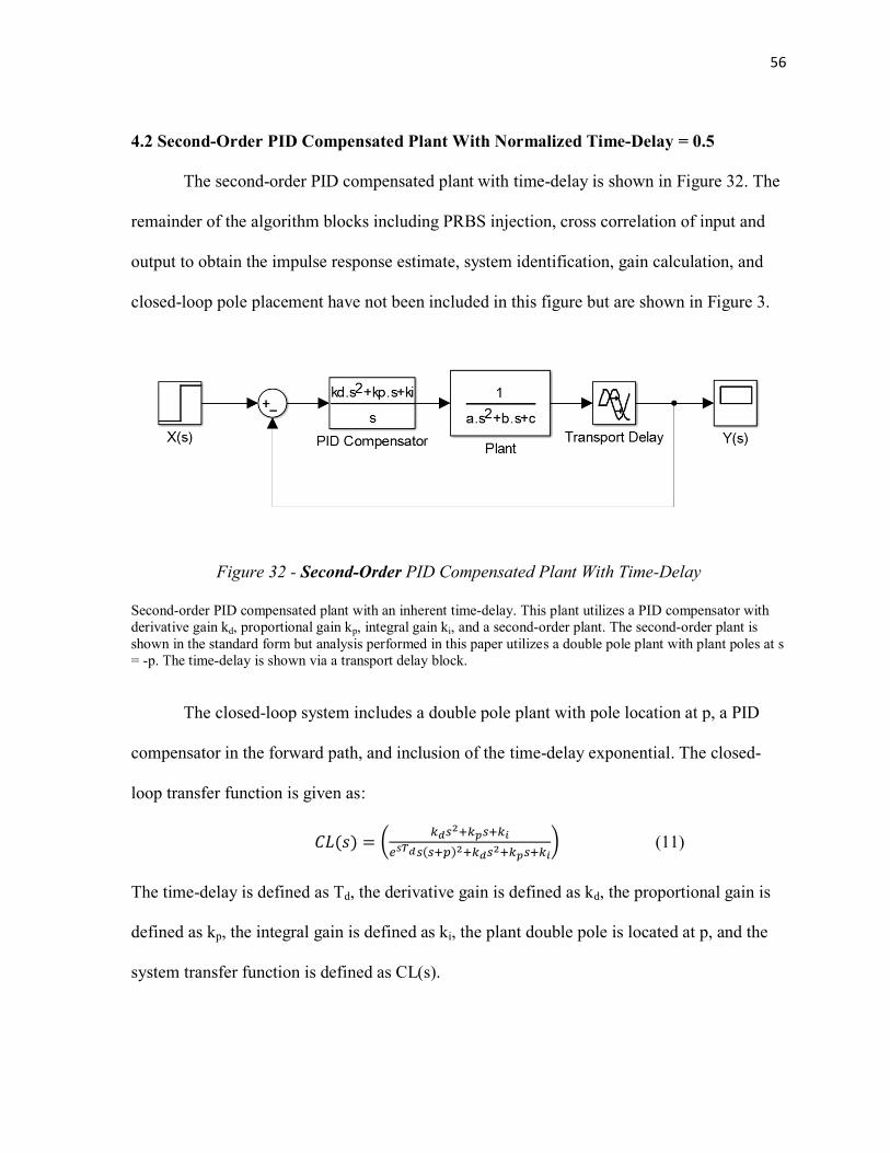
56

4.2 Second-Order PID Compensated Plant With Normalized Time-Delay = 0.5

The second-order PID compensated plant with time-delay is shown in Figure 32. The

remainder of the algorithm blocks including PRBS injection, cross correlation of input and

output to obtain the impulse response estimate, system identification, gain calculation, and

closed-loop pole placement have not been included in this figure but are shown in Figure 3.

Figure 32 - Second-Order PID Compensated Plant With Time-Delay

Second-order PID compensated plant with an inherent time-delay. This plant utilizes a PID compensator with

derivative gain kd, proportional gain kp, integral gain ki, and a second-order plant. The second-order plant is

shown in the standard form but analysis performed in this paper utilizes a double pole plant with plant poles at s

= -p. The time-delay is shown via a transport delay block.

The closed-loop system includes a double pole plant with pole location at p, a PID

compensator in the forward path, and inclusion of the time-delay exponential. The closed-

loop transfer function is given as:

(11)

The time-delay is defined as Td, the derivative gain is defined as kd, the proportional gain is

defined as kp, the integral gain is defined as ki, the plant double pole is located at p, and the

system transfer function is defined as CL(s).

57

The test system utilized for this demonstration has a double plant pole at s = -3, a

double compensator zero at s = -4, a loop gain of 2, a time-delay of 0.167 seconds, and an

NTD of 0.5. A 15-bit PRBS with an amplitude of 1 was injected into the system over a time

period of 250 seconds to identify the system, assess the time-delay, place the compensator

zeros and adjust the loop gain to achieve the commanded overshoot. One-hundred seconds of

the output of the system due to PRBS injection is shown in Figure 33. The estimated impulse

response is shown in Figure 34.

Figure 33 - System Output for Second-Order PID Compensated System With Time-Delay

Due to Pseudo-Random Binary Sequence Injection

This figure shows the system output when a 15-bit PRBS with an amplitude of 1 is injected into the system.

This system has a loop gain of 2, a double compensator zero placed at s = -4, double plant poles at s = -3 and a

time-delay of 0.167 seconds. This corresponds to an NTD of 0.5.

0 20 40 60 80 100

-0.6

-0.4

-0.2

0

0.2

0.4

0.6

Time (s)

Outp

ut

(Am

plitu

de

)

System Output

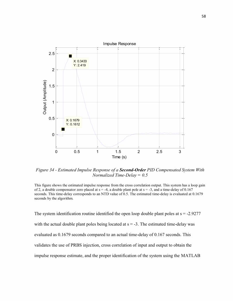
58

Figure 34 - Estimated Impulse Response of a Second-Order PID Compensated System With


This figure shows the estimated impulse response from the cross correlation output. This system has a loop gain

of 2, a double compensator zero placed at s = -4, a double plant pole at s = -3, and a time-delay of 0.167

seconds. This time-delay corresponds to an NTD value of 0.5. The estimated time-delay is evaluated at 0.1679

seconds by the algorithm.

The system identification routine identified the open loop double plant poles at s = -2.9277

with the actual double plant poles being located at s = -3. The estimated time-delay was

evaluated as 0.1679 seconds compared to an actual time-delay of 0.167 seconds. This

validates the use of PRBS injection, cross correlation of input and output to obtain the

impulse response estimate, and the proper identification of the system using the MATLAB

0 0.5 1 1.5 2 2.5 3

0

0.5

1

1.5

2

2.5

X: 0.3433

Y: 2.419

Time (s)

Outp

ut

(Am

plitu

de

)Impulse Response

X: 0.1679

Y: 0.1612

59

lsqcurevefit() function for a second-order system with time-delay. The Bode plot of the

frequency response is shown in Figure 35.


Cross-Correlation (blue) of a Second-Order PID Compensated System With





estimated frequency response data. The phase plot does not stabilize at a certain value but rolls off as frequency

increases due to the time-delay exponential.

Since the system is identified as a double pole plant with s = -2.9277, the PID

compensator zeros are placed slightly off, at s = -3.2205, -2.6349. This is evidenced in the

10-2

10-1

100

101

102

103

-60

-40

-20

0

20

Mag

nitu

de (

dB

)

Frequency (rad/s)


10-2

10-1

100

101

102

103

-6000

-4000

-2000

0

2000

Pha

se (

de

gre

es)

Frequency (rad/s)

60

slightly lower overshoots seen in the output responses compared to the ideal results seen in

Figures 17 and 18. In this case, all overshoot results are within 5% of the commanded values

as shown in Figure 36.

Figure 36 - Step Response Outputs for a Second-Order PID Compensated Plant Tuned for

Commanded Overshoots of 0, 5, 10, 15, and 20%

System step response results after tuning for various commanded overshoots. It is important to note that the

overshoots do not match the commanded overshoots seen in Figures 17 and 18 due to the error in the

identification of the double plant pole. The actual overshoots observed, however, match the commanded results

within 5%.

0 0.5 1 1.5 20

0.2

0.4

0.6

0.8

1

1.2

Step Response

Time (seconds)

Am

plit

ud

e

0%

5%

10%

15%

20%

Overshoot

61

4.3 First-Order PI Compensated Plant With Normalized Time-Delay = 1

As a justification for this method it is important to look beyond what has been done in

previous work (Baker, 2011). For NTD > 0.5, auto tuning has not been adequately explored.

In a situation like this it is easy to come up with an example of why a system like this is

important to understand. For example, if there was a well tuned system that was stable at a

specific operating condition, it could become unstable with a slow drift in time-delay. The

auto tuning algorithm would be able to ensure the system remained stable and adjust the

performance to maintain the commanded overshoot.

For example, the system from the first-order results section, with a plant pole of s =

-4, is tuned using the auto tuning algorithm and exhibits a typical response of approximately

10% overshoot after tuning. If the time-delay inherent in the system is increased, from NTD

= 0.5 to 1, the system dynamics will change and re-tuning will need to occur for proper

operation. In this case the time-delay increase, leads to oscillatory behavior, as shown in

Figure 37.

By re-applying the tuning algorithm to the system, it may no longer be possible to

achieve a response that is comparable to the plant pole response, but at least the system will

be tuned to be stable and maintain an overshoot that meets the design specifications of the

system. By re-applying the auto-tuning method, the acceptable response shown in Figure 38

is achieved.

This result shows that the system can be maintained in a properly tuned state as time-

delay is changed. This result shows that a system can still be stabilized with an optimum

performance given a large time-delay that is on the order of the plant time constant. With

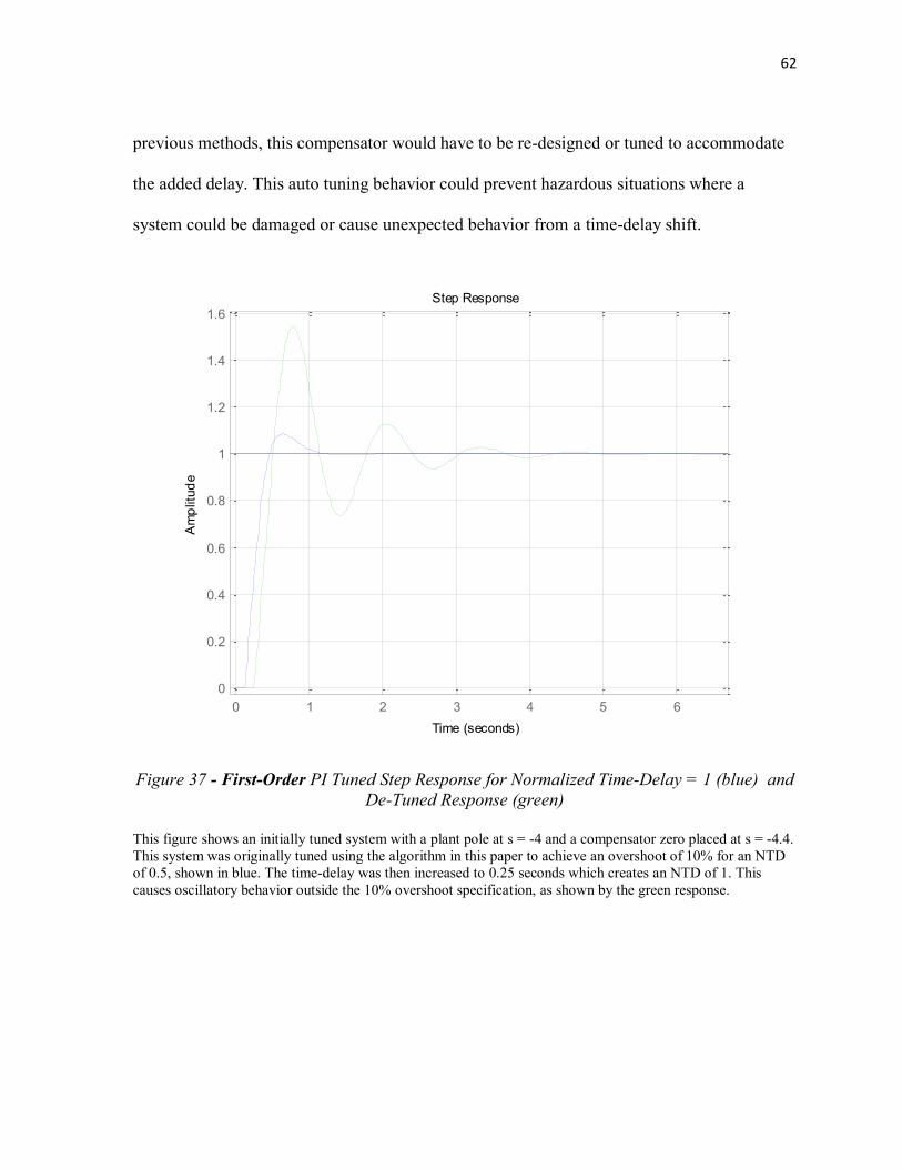
62

previous methods, this compensator would have to be re-designed or tuned to accommodate

the added delay. This auto tuning behavior could prevent hazardous situations where a

system could be damaged or cause unexpected behavior from a time-delay shift.

Figure 37 - First-Order PI Tuned Step Response for Normalized Time-Delay = 1 (blue) and

De-Tuned Response (green)

This figure shows an initially tuned system with a plant pole at s = -4 and a compensator zero placed at s = -4.4.

This system was originally tuned using the algorithm in this paper to achieve an overshoot of 10% for an NTD

of 0.5, shown in blue. The time-delay was then increased to 0.25 seconds which creates an NTD of 1. This

causes oscillatory behavior outside the 10% overshoot specification, as shown by the green response.

0 1 2 3 4 5 6

0

0.2

0.4

0.6

0.8

1

1.2

1.4

1.6

Step Response

Time (seconds)

Am

plit

ud

e

63

Figure 38 - First-Order PI Compensated System With Oscillatory Response (blue) and Re-

Tuned Response (green)

This figure shows the oscillatory response from the previous figure in blue, which was a response for the de-

tuned system at an NTD of 1. This green response shows the response after re-tuning which matches the

original overshoot by sacrificing the time response.

0 1 2 3 4 5 6

0

0.5

1

1.5

Step Response

Time (seconds)

Am

plit

ud

e

64

4.4 Second-Order PID Compensated Plant With Normalized Time-Delay = 1

The second-order PID compensated Plant can be shown to exhibit similar behavior

when a larger time-delay is introduced. In this case, a second-order plant with double poles at

s = -3 is utilized to demonstrate the algorithm. This plant has been previously compensated

utilizing the real-time auto tuning algorithm and exhibits the behavior shown in Figure 39.

This figure shows the plant as tuned for an NTD of 0.5 and the de-tuned plant with an NTD

of 1. As was seen in the last section, it is possible to re-tune the plant by running it through

the auto tuning algorithm. Figure 40 shows similar results to the first-order plant in that the

system overshoot is reduced with a slight sacrifice in the system speed.

65

Figure 39 - Second-Order PID Tuned Step Response for Normalized Time-Delay = 1 (blue)

and De-Tuned Response (green)

This figure shows the originally tuned plant response for a second-order system with double plant poles at s = -3

in blue. By increasing the time-delay to 0.33 seconds, corresponding to an NTD of 1, the plant exhibits

oscillatory behavior due to the time-delay, as shown in green.

0 1 2 3 4 5 6 7 8 9

0

0.2

0.4

0.6

0.8

1

1.2

1.4

1.6

Step Response

Time (seconds)

Am

plit

ud

e

66

Figure 40 - Second-Order PID Compensated System With Oscillatory Response (blue) and

Re-Tuned Response (green)

This plot shows a second-order PID compensated plant response which has been de-tuned by increasing the

time-delay to 0.33 seconds, corresponding to an NTD of 1, shown in blue. The plant is then re-tuned using the

algorithm discussed in this work, shown in green, by sacrificing plant time response to achieve an overshoot

reduction.

0 1 2 3 4 5 6 7 8 9 10

0

0.2

0.4

0.6

0.8

1

1.2

1.4

1.6

Step Response

Time (seconds)

Am

plit

ud

e

67

5. Conclusion

This paper presents the results of a real-time auto tuning method for first and second-

order systems with time-delay using PRBS and the cross-correlation method. A PRBS was

used to excite the dominant modes of the system to produce an estimate of the impulse

response via the cross correlation of the input PRBS with the output of the closed-loop

system. The estimate of the impulse response contains the dominant dynamics of the closed-

loop system and can be used to develop an estimate of the system's closed-loop transfer

function and the time-delay. The time-delay is estimated using the maximum point in the

derivative of the estimated impulse response. The FFT of the impulse response is taken to

obtain an estimate of the frequency response of the system. This result is compared to the

known form of the closed-loop transfer function for a first or second-order system with time-

delay. The estimated frequency response data is compared to a model function using the

MATLAB lsqcurvefit() function, which varies the plant pole location until it finds a

minimum in the mean square error between the data and model function. This method

utilizes a single search gradient descent method and an optimization function, that takes into

account the current PID parameters, the estimated time-delay, and the appropriate form for

the closed-loop transfer function. The estimated plant pole location and estimated time-delay

are then used for compensator placement based on iterative tuning results shown in Tables 1

and 2 and the desired overshoot for the system.

The PRBS and cross-correlation portion of this real-time auto tuning algorithm

required a decision about which size of PRBS to use and the length of time data that would

68

be used for analysis. The longer the set of time data that the PRBS is being applied over, the

more accurate the impulse response estimate will be. As the length of the time data gets

shorter, the cross-correlation process will suffer from more artifacts in the system output

which leads to a difficult system to analyze. The size of PRBS attempts to balance these

competing factors to provide an acceptable time resolution and frequency resolution, while

maximizing the accuracy of the estimated impulse response. The size of the PRBS was

chosen as a 15-bit generator applied over a 250 second set of data, which provides for a time

resolution of 7.6 milli-seconds and frequency dynamics up to 411.74 rad/sec. In this range,

there are still artifacts from the cross correlation process but the system is still identifiable

with a relatively short data sample. These parameters could be adjusted to apply the method

to a different range of systems by changing the number of bits in the PRBS or the length of

time data utilized. The results in this research show that the PRBS frequency content was

sufficiently rich to properly excite the example systems and achieve an accurate estimate of

the impulse response and time-delay.

The system identification routine, utilized in this algorithm, was a MATLAB function

that provides curve fitting using a Gradient Descent regression technique. The lsqcurvefit()

function was used to compare the estimated frequency response data to the model transfer

function and adjusted the plant pole parameter until the best fit was found. This comparison

utilized a minimization of the mean square error based on an initial starting point determined

by experimentation. It was found that the starting point for the regression technique needed

to be large compared to the plant pole, so it was chosen above the frequency range that the

system was designed to analyze. This ensures that the descent along the mean square error

69

curve has the best chance of converging to the global minimum, and minimizes the chance

that a local minimum would be found instead. The system identification routine was able to

estimate the plant poles reliably and provide these poles to the compensator tuning portion of

the algorithm.

The final portion of the algorithm involved the gain calculation based on a consistent

compensator zero placement. By starting with the PID tuning method proposed by Baker

(2011) a modified compensator zero placement method was developed to achieve a specific

overshoot, based on the system time-delay. By consistently placing the compensator zeros at

1.1 times the plant pole for a first-order system, and 1.1 and 0.9 times the plant pole for a

second-order system, the root locus generated using the time-delay exponential showed

consistent behavior for each NTD value. This result was leveraged by iteratively tuning test

systems to achieve a specific overshoot and relationships between overshoot, time-delay,

and loop gain were developed. Tables 1 and 2 provide these relationships and are utilized in

the auto tuning algorithm to reliably place the closed-loop poles to achieve a user

commanded overshoot. The results of these relationships provide auto tuning results for an

identified system within 5% of the commanded overshoot.

The results of this research demonstrate that the real-time auto tuning algorithm for a

first or second-order system with time-delay is a viable method. The MATLAB routines that

were written to simulate the behavior of the system and the results of each piece of the

algorithm worked independently, as shown in the development section. They also worked

together, as shown in the validation and results sections. The algorithm results were

70

consistent with the goal of tuning the system to within 5% of the commanded overshoot and

show that PRBS injection for system identification and automatic tuning of a time-delayed

system is possible.

71

6. Discussion

This research was a first step in the development of a real-time auto tuning algorithm

for a first or second-order system with time-delay, but there are a few issues that warrant

further investigation and improvement. This study was theoretically based and all results

were obtained utilizing MATLAB simulation software. In real systems, there are many other

aspects that need to be taken into account, including

System noise

Disturbance rejection

Accuracy of system identification

Algorithm tradeoffs

Hardware implementation

Many of these issues have been addressed in previous research, but the ideas need to be

consolidated and applied to the real-time auto tuning algorithm presented in this paper.

System noise is inherent in all systems due to the use of electronic amplifiers,

computers, and the heating up of system components. With respect to the way that time-delay

and noise interact, research has been conducted by Yue and Han (2005) that introduces

important points which could be incorporated into the algorithm to make it more robust.

Noise could also be reduced by averaging techniques that utilize multiple periods of PRBS

signals, with different starting seed values, as demonstrated by Sohrab, Reischl, Grodins, and

Yamashiro's application to respiratory systems (1978). This process takes longer to gather

72

the data, but it will effectively reduce noise in the output as the output sequences are

averaged together.

The next issue that was not addressed in this research is the disturbance rejection

ability of the tuned system. The tuning of the system to achieve a desired overshoot does not

take into account what will happen if there is a load disturbance applied to the system. The

overshoot in the response to a step input may be adequate but there are tradeoffs that need to

be made to balance the step response and the load disturbance rejection. The system may be

well-tuned with respect to an overshoot for a step response but a load change may show a

much larger response, which could cause undesirable excursion from the setpoint and

possible damage to the system. In Baker's approach to compensator tuning (2011) these

issues were discussed and could be applied in the future application of this algorithm.

The largest weakness of the algorithm was the identification of the plant poles of the

system. Even a small error in the estimated plant pole location may cause the compensator

zeros to be placed inappropriately for the system, which will lead to an offset in the

commanded overshoot observed in the step response. This behavior is shown in the

differences between figures 31 and 15 for a first-order system with time-delay, and figures 36

and 17 for a second-order system with time-delay. This result could be improved by

performing a multiple starting point gradient descent technique and averaging the results, or

by creating a smarter search algorithm that was customized to the application. By enhancing

the implementation of the system identification algorithm, the identification results could be

73

greatly improved, which would directly translate to more accurate compensation

performance.

There was some comparison performed between the Baker method (2011) of

compensator placement and the method proposed in this paper. However, there was not a

discussion as to whether one method was preferred over the other for specific NTD

situations. As was mentioned in this paper, the Baker method provides inferior results for

NTD greater than 0.5. However, the Baker method may provide better results for NTD < 0.5.

The goal of this paper was not to explore an optimized algorithm but to present new results

for a broader range of NTD than had been previously addressed. An important next step to

the development of an optimized algorithm would be to analyze the tradeoffs between

different compensation methods and include decision making points in the algorithm to use

the method that is most optimal for the situation. The Baker method and the method explored

in this paper are only two compensation methods that have been explored so it is also

important to experiment with other compensation techniques that could yield better results.

The hardware implementation of this real-time auto tuning system is another issue

that was not adequately discussed in this research. The algorithm claims to be a real-time

auto tuning algorithm but, in reality, it is not feasible to adjust the gain for every new data

sample taken. The calculations could be performed in real-time to produce a real-time gain

recommendation but it would be impractical to update the compensator values in real-time.

Updating the gain value continuously could even cause system instability if the compensator

was not placed appropriately due to a cascade effect from the gain changes. This algorithm is

74

real-time in a buffered sense because an adequate data sample needs to be collected before

the first gain calculation can be run. The system could be continuously updating the cross

correlation result, running the system identification routine, and calculating the required loop

gain but there would need to be decision logic added to decide when to update the

compensator locations.

This research validates the feasibility of the proposed method and the algorithm meets

the overshoot performance specified. There are still improvements that can be made and

issues that need to be addressed for further optimization and development.

75

References

Astrom, K. J., & Hagglund, T. (1995). PID controllers: Theory, design, & tuning. Research

Triangle Park, N.C.: International Society for Measurement and Control.

Baker, G. (2011). PID-Tuning of plants with time delay using root locus. (Master's thesis).

Retrieved from SJSU ScholarWorks. (Paper 4036).

Bahill, A. T. (1983). A simple adaptive smith-predictor for controlling time-delay systems.

Control Systems Magazine, IEEE, 3(2), pp 16-22. doi:10.1109/MCS.1983.1104748

Frazzoli, E. (2010). Time Delays. Retrieved from http://ocw.mit.edu/courses/aeronautics-and-

astronautics/16-30-feedback-control- systems-fall-2010/recitations/

MIT16_30F10_rec11.pdf

, M. (2011). Identification of dynamic systems: An introduction

with applications. Heidelberg, N.Y.: Springer.

Miao, B., Zane, R., & Maksimovic, D. (2004). A modified cross-correlation method for

system identification of power converters with digital control. Power Electronics

Specialists Conference, IEEE, 5, pp 3728-3733. doi:10.1109/PESC.2004.1355134

Ogata, K. (2002). Modern control engineering (4th ed.). Upper Saddle River, N.J.: Prentice

Hall.

Oppenheim, A. V., & Schafer, R. W. (2010). Discrete-time signal processing. Upper

Saddle River: Pearson.

Sipahi, R., Niculescu, S., Abdallah, C., Michiels, W., & Gu, K. (2011). Stability and

stabilization of systems with time delay. Control Systems, IEEE, 31(1), pp 38-65.

doi:10.1109/MCS.2010.939135

Sohrab, S., Reischl, P., Grodins, F. S., & Yamashiro, S. M. (1978). Application of pseudo

random binary sequence input to identification of respiratory control dynamics.

Decision and Control, IEEE, 17, pp 1304-1308. doi:10.1109/CDC.1978.268130

76

Vajta, M. (2000). Some remarks on Padé-Approximations. 3rd Tempus-Intcom

Symposium, Vezprem, Hungary, 1–6.

Yue, D., & Han, Q. (2005). Delay-Dependent exponential stability of stochastic systems

with time-varying delay, nonlinearity, and markovian switching. Automatic

Control, IEEE Transactions, 50(2), pp 217-222. doi:10.1109/TAC.2004.841935

Ziegler, J. G., & Nichols, N. B. (1942). Optimum settings for automatic controllers.

Transactions of the ASME, pp 759–765.

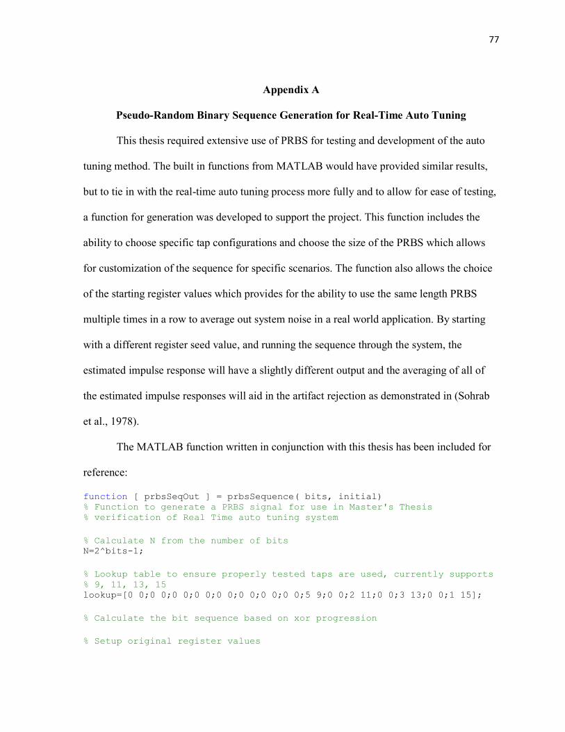
77

Appendix A

Pseudo-Random Binary Sequence Generation for Real-Time Auto Tuning

This thesis required extensive use of PRBS for testing and development of the auto

tuning method. The built in functions from MATLAB would have provided similar results,

but to tie in with the real-time auto tuning process more fully and to allow for ease of testing,

a function for generation was developed to support the project. This function includes the

ability to choose specific tap configurations and choose the size of the PRBS which allows

for customization of the sequence for specific scenarios. The function also allows the choice

of the starting register values which provides for the ability to use the same length PRBS

multiple times in a row to average out system noise in a real world application. By starting

with a different register seed value, and running the sequence through the system, the

estimated impulse response will have a slightly different output and the averaging of all of

the estimated impulse responses will aid in the artifact rejection as demonstrated in (Sohrab

et al., 1978).

The MATLAB function written in conjunction with this thesis has been included for

reference:

function [ prbsSeqOut ] = prbsSequence( bits, initial) % Function to generate a PRBS signal for use in Master's Thesis % verification of Real Time auto tuning system

% Calculate N from the number of bits N=2^bits-1;

% Lookup table to ensure properly tested taps are used, currently supports % 9, 11, 13, 15 lookup=[0 0;0 0;0 0;0 0;0 0;0 0;0 0;0 0;5 9;0 0;2 11;0 0;3 13;0 0;1 15];

% Calculate the bit sequence based on xor progression

% Setup original register values

78

registerValues=initial;

% Cycle through using taps and shift registers and create the bit sequence for i=1:N prbsSeq(i)=registerValues(bits);

temp=xor(registerValues(lookup(bits,1)),registerValues(lookup(bits,2))); for j=1:bits-1 registerValues(bits+1-j)=registerValues(bits-j); end registerValues(1)=temp; end

% Output the sequence for use in other functions prbsSeqOut=prbsSeq;

end

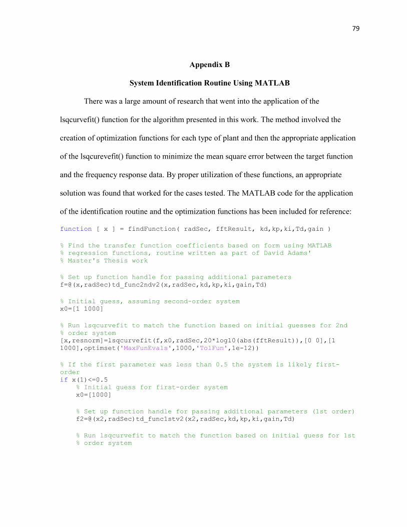
79

Appendix B

System Identification Routine Using MATLAB

There was a large amount of research that went into the application of the

lsqcurvefit() function for the algorithm presented in this work. The method involved the

creation of optimization functions for each type of plant and then the appropriate application

of the lsqcurevefit() function to minimize the mean square error between the target function

and the frequency response data. By proper utilization of these functions, an appropriate

solution was found that worked for the cases tested. The MATLAB code for the application

of the identification routine and the optimization functions has been included for reference:

function [ x ] = findFunction( radSec, fftResult, kd,kp,ki,Td,gain )

% Find the transfer function coefficients based on form using MATLAB % regression functions, routine written as part of David Adams' % Master's Thesis work

% Set up function handle for passing additional parameters f=@(x,radSec)td_func2ndv2(x,radSec,kd,kp,ki,gain,Td)

% Initial guess, assuming second-order system x0=[1 1000]

% Run lsqcurvefit to match the function based on initial guesses for 2nd % order system [x,resnorm]=lsqcurvefit(f,x0,radSec,20*log10(abs(fftResult)),[0 0],[1

1000],optimset('MaxFunEvals',1000,'TolFun',1e-12))

% If the first parameter was less than 0.5 the system is likely first-

order if x(1)<=0.5 % Initial guess for first-order system x0=[1000]

% Set up function handle for passing additional parameters (1st order) f2=@(x2,radSec)td_func1stv2(x2,radSec,kd,kp,ki,gain,Td)

% Run lsqcurvefit to match the function based on initial guess for 1st % order system

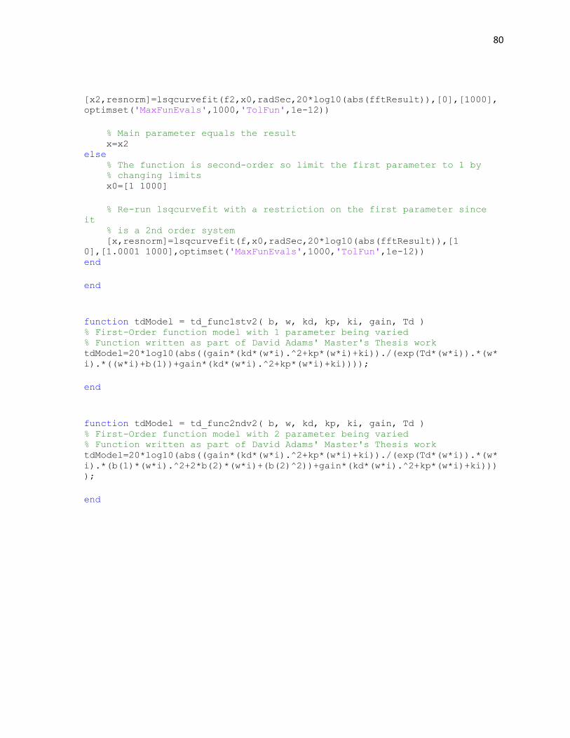
80

[x2,resnorm]=lsqcurvefit(f2,x0,radSec,20*log10(abs(fftResult)),[0],[1000],

optimset('MaxFunEvals',1000,'TolFun',1e-12))

% Main parameter equals the result x=x2 else % The function is second-order so limit the first parameter to 1 by % changing limits x0=[1 1000]

% Re-run lsqcurvefit with a restriction on the first parameter since

it % is a 2nd order system [x,resnorm]=lsqcurvefit(f,x0,radSec,20*log10(abs(fftResult)),[1

0],[1.0001 1000],optimset('MaxFunEvals',1000,'TolFun',1e-12)) end

end

function tdModel = td_func1stv2( b, w, kd, kp, ki, gain, Td ) % First-Order function model with 1 parameter being varied % Function written as part of David Adams' Master's Thesis work tdModel=20*log10(abs((gain*(kd*(w*i).^2+kp*(w*i)+ki))./(exp(Td*(w*i)).*(w*

i).*((w*i)+b(1))+gain*(kd*(w*i).^2+kp*(w*i)+ki))));

end

function tdModel = td_func2ndv2( b, w, kd, kp, ki, gain, Td ) % First-Order function model with 2 parameter being varied % Function written as part of David Adams' Master's Thesis work tdModel=20*log10(abs((gain*(kd*(w*i).^2+kp*(w*i)+ki))./(exp(Td*(w*i)).*(w*

i).*(b(1)*(w*i).^2+2*b(2)*(w*i)+(b(2)^2))+gain*(kd*(w*i).^2+kp*(w*i)+ki)))

);

end

81

Appendix C

Algorithm for Real-Time Auto Tuning With Time-Delay

The actual algorithm that was run for the real-time auto tuning validation and testing

ties together all of the sub topics contained in this thesis. This function assumes that the user

has already collected the data from the system and is ready to pass that data to the auto tuning

algorithm. This algorithm takes in the data, along with the known system parameters, and a

commanded overshoot and returns the tuned PID values to place the compensator and the

loop gain to achieve the commanded overshoot. This function computes sampling frequency

and sample time to properly scale the FFT results and computes the frequency data needed

for system identification. The algorithm then runs the system identification routine as

discussed in Appendix B. Once the system is identified, the algorithm prints out the Bode

Plots and calculates the compensator zero placement and the corresponding gain for the

system. This result is then returned to be applied to the system to achieve a satisfactory

response. The MATLAB algorithm written for this method has been included for reference

and contains the gain calculation section near the end of the algorithm.

function [ kTune gainTuned ] = pidAutoTuning( t, inputs, outputs, kd, kp,

ki, gain, overshoot ) % PID auto tuning method written by David Adams for validation of the auto

tuning method % developed for Master's Thesis

% Find the impulse response by cross-correlation output=getImpulse(inputs, outputs, t);

% Evaluate the time delay of the impulse response for use in regression % analysis Td=tdevalv2(t, output);

% Set up other important parameters for evaluation

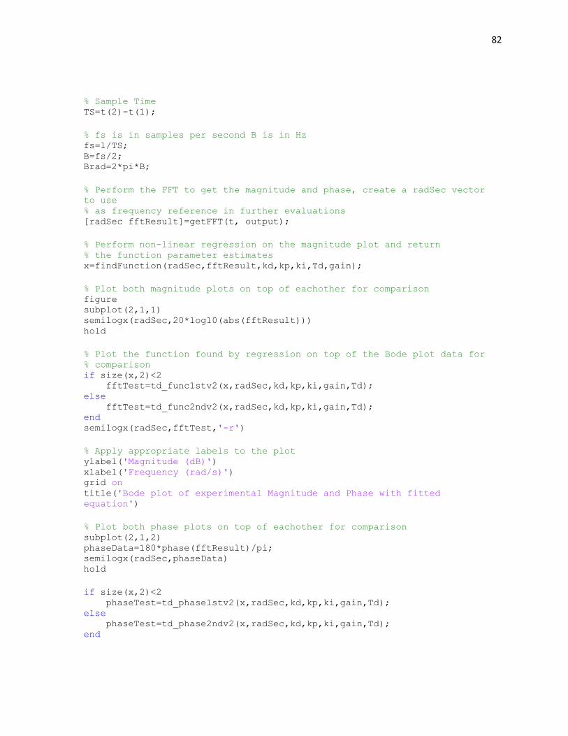
82

% Sample Time TS=t(2)-t(1);

% fs is in samples per second B is in Hz fs=1/TS; B=fs/2; Brad=2*pi*B;

% Perform the FFT to get the magnitude and phase, create a radSec vector

to use % as frequency reference in further evaluations [radSec fftResult]=getFFT(t, output);

% Perform non-linear regression on the magnitude plot and return % the function parameter estimates x=findFunction(radSec,fftResult,kd,kp,ki,Td,gain);

% Plot both magnitude plots on top of eachother for comparison figure subplot(2,1,1) semilogx(radSec,20*log10(abs(fftResult))) hold

% Plot the function found by regression on top of the Bode plot data for % comparison if size(x,2)<2 fftTest=td_func1stv2(x,radSec,kd,kp,ki,gain,Td); else fftTest=td_func2ndv2(x,radSec,kd,kp,ki,gain,Td); end semilogx(radSec,fftTest,'-r')

% Apply appropriate labels to the plot ylabel('Magnitude (dB)') xlabel('Frequency (rad/s)') grid on title('Bode plot of experimental Magnitude and Phase with fitted

equation')

% Plot both phase plots on top of eachother for comparison subplot(2,1,2) phaseData=180*phase(fftResult)/pi; semilogx(radSec,phaseData) hold

if size(x,2)<2 phaseTest=td_phase1stv2(x,radSec,kd,kp,ki,gain,Td); else phaseTest=td_phase2ndv2(x,radSec,kd,kp,ki,gain,Td); end

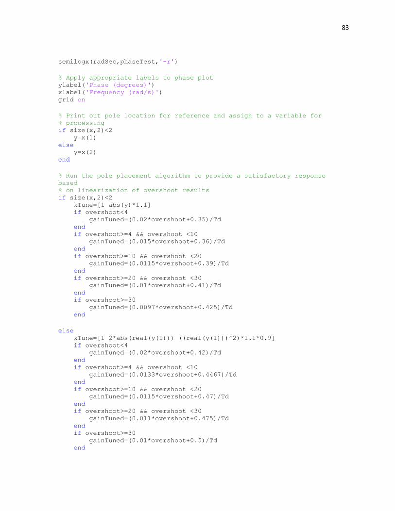
83

semilogx(radSec,phaseTest,'-r')

% Apply appropriate labels to phase plot ylabel('Phase (degrees)') xlabel('Frequency (rad/s)') grid on

% Print out pole location for reference and assign to a variable for % processing if size(x,2)<2 y=x(1) else y=x(2) end

% Run the pole placement algorithm to provide a satisfactory response

based % on linearization of overshoot results if size(x,2)<2 kTune=[1 abs(y)*1.1] if overshoot<4 gainTuned=(0.02*overshoot+0.35)/Td end if overshoot>=4 && overshoot <10 gainTuned=(0.015*overshoot+0.36)/Td end if overshoot>=10 && overshoot <20 gainTuned=(0.0115*overshoot+0.39)/Td end if overshoot>=20 && overshoot <30 gainTuned=(0.01*overshoot+0.41)/Td end if overshoot>=30 gainTuned=(0.0097*overshoot+0.425)/Td end

else kTune=[1 2*abs(real(y(1))) ((real(y(1)))^2)*1.1*0.9] if overshoot<4 gainTuned=(0.02*overshoot+0.42)/Td end if overshoot>=4 && overshoot <10 gainTuned=(0.0133*overshoot+0.4467)/Td end if overshoot>=10 && overshoot <20 gainTuned=(0.0115*overshoot+0.47)/Td end if overshoot>=20 && overshoot <30 gainTuned=(0.011*overshoot+0.475)/Td end if overshoot>=30 gainTuned=(0.01*overshoot+0.5)/Td end

84

end

% Function returns the recommended tuning parameters and the recommended % gain found by the auto tuning algorithm

end

Real-time Auto Tuning of a Closed Loop Second Order System ...

Documents

Transcript of Real-time Auto Tuning of a Closed Loop Second Order System ...