Re-thinking the housing-macro nexus: housing market churn ... · partial wavelet based statistics...
39
Bazil Sansom / 21 st FMM Conference “The Crisis of Globalisation”, Berlin 9-11 November 2017 Re-thinking the housing-macro nexus: housing market churn in aggregate demand formation and stability, a wavelets based analysis. Bazil A. Sansom Abstract I take a data driven approach to investigating the relationship between housing and macroeconomic cycles for the US economy. I use wavelet power and coherence spectra for housing and GDP series to identify the spectral ranges of and relationship between housing and GDP cycles. To unpack these relationships I then employ a ‘network discovery’ procedure, deploying bivariate and partial wavelet based statistics combined with graph theoretic methods to identify a network projection of nontrivial relationships between a detailed set of housing, financial and macro variables over an identified cycle frequency range. Finally I make a detailed wavelet based time-frequency domain study of those links identified as key relationships by the network-discovery procedure. My results confirm the importance of housing in US macroeconomic cycles at low frequencies, and identify secondary housing market volumes (existing homes) as a global “source”, thus candidate ‘root cause’ of low frequency cycles, propagating most directly to the wider economy via residential investment and durable- consumption. This raises the unexpected possibility that secondary housing market volumes - a variable unconsidered in the theoretical or empirical literature - may be an autonomous source of fluctuations, and lead a significant low-frequency macroeconomic cycle. 1 Introduction Study of the macroeconomic cycle has long emphasised the ‘business cycle’. However not only was the US housing market conspicuously implicated in the 2007-8 crisis, but a growing body of mostly statistically driven empirical work seems to implicate housing much more widely in economic cycles and instability. There is a now well established long running association between housing market boom-bust and systemic banking crises (Borio and Drehmann 2009; Crowe et al. 2013; IMF 2012; IMF et al. 2012; Kindleberger and Aliber 2005). Credit growth is a powerful predictor of financial crises in advanced economies (Reinhart and Rogoff 2011; Schularick and Taylor 2009) and house prices and household credit in particular emerge as one of the best leading indicators (Alessi et al. 2014; Alessi and Detken 2009; Borio 2014; Borio and Drehmann
Transcript of Re-thinking the housing-macro nexus: housing market churn ... · partial wavelet based statistics...

Bazil Sansom / 21st FMM Conference “The Crisis of Globalisation”, Berlin 9-11 November 2017
Re-thinkingthehousing-macronexus:housingmarketchurninaggregatedemandformationand
stability,awaveletsbasedanalysis.
BazilA.Sansom
Abstract
I take a data driven approach to investigating therelationshipbetweenhousingandmacroeconomiccyclesfor theUSeconomy. IusewaveletpowerandcoherencespectraforhousingandGDPseriestoidentifythespectralranges of and relationship between housing and GDPcycles. To unpack these relationships I then employ a‘network discovery’ procedure, deploying bivariate andpartial wavelet based statistics combined with graphtheoretic methods to identify a network projection ofnontrivialrelationshipsbetweenadetailedsetofhousing,financial and macro variables over an identified cyclefrequencyrange.FinallyImakeadetailedwaveletbasedtime-frequencydomainstudyof those links identifiedaskey relationships by the network-discovery procedure.My results confirm the importance of housing in USmacroeconomic cycles at low frequencies, and identifysecondaryhousingmarketvolumes(existinghomes)asaglobal “source”, thus candidate ‘root cause’ of lowfrequencycycles,propagatingmostdirectly to thewidereconomy via residential investment and durable-consumption. This raises theunexpectedpossibility thatsecondary housing market volumes - a variableunconsidered in the theoretical or empirical literature -maybeanautonomoussourceoffluctuations,andleadasignificantlow-frequencymacroeconomiccycle.
1 IntroductionStudy of the macroeconomic cycle has long emphasised the ‘business cycle’.Howevernot onlywas theUShousingmarket conspicuously implicated in the2007-8crisis,butagrowingbodyofmostly statisticallydrivenempiricalworkseemstoimplicatehousingmuchmorewidelyineconomiccyclesandinstability.There is a now well established long running association between housingmarket boom-bust and systemic banking crises (Borio and Drehmann 2009;Crowe et al. 2013; IMF 2012; IMF et al. 2012; Kindleberger and Aliber 2005).Creditgrowthisapowerfulpredictoroffinancialcrisesinadvancedeconomies(Reinhart andRogoff2011; SchularickandTaylor2009)andhouseprices andhousehold credit in particular emerge as one of the best leading indicators(Alessi et al. 2014; Alessi andDetken 2009; Borio 2014; Borio andDrehmann

Bazil Sansom / 21st FMM Conference “The Crisis of Globalisation”, Berlin 9-11 November 2017
2009; Borio and Lowe 2002; Büyükkarabacak and Valev 2010; Davis and Zhu2004;DufrénotandMalik2012;Szemere,Scatigna,andTsatsaronis2014)withmortgagedebtdrivencreditboomsmorelikelyto‘gobad’(BezemerandZhang2014; Jorda, Schularick, and Taylor 2014). There is evidence that in manyadvanced economies household debt (Barbosa-filho et al. 2008) house prices(Borio 2014; Goodhart and Hofmann 2008; IMF 2008; IMF et al. 2009) andresidential investment in particular (Álvarez and Cabrero 2010; Davis andHeathcote2005;FerraraandVigna2009;Iganetal.2011;IMF2008;IMFetal.2009; Kydland, Rupert, and Sustek 2016; Leamer 2007)1appear to lead the“business cycle”. What is more a large and growing body of empirical worksuggests that recessions preceded by larger increases in household debt(principallymortgagecredit)tendtobemoresevereandprotracted(AdalidandDetken 2007; IMF et al. 2012; Jorda, Schularick, and Taylor 2012; Jorda et al.2014;JuseliusandDrehmann2015;King1994;Mian,Sufi,andVerner2015)andthatrecessionsassociatedwithhousepricebuststendtobedeeperandlonger(Claessens et al. 2012). Taken together, these various strands in the empiricalliterature underscore a need to clarify and deepen our understanding of therelationshipbetweenhousingcyclesandmacroeconomiccycles.Though long studied in economics, understanding cycles and instabilitycontinuestoposeaconsiderableandkeychallenge.Economiccyclespotentiallyarise for a variety of reasons - the propagation of shocks or the emergence ofendogenous cyclicality through the interactions between economic processes.Thehighlyinterconnectedandcomplexnatureofthesystemmeansthatonceanoscillation is generated somewhere in theeconomy, itmayeasilypropagate tootherparts,makingtherootcausesofmacroeconomiccyclesdifficulttoidentify.The complex spectral content, and very often non-stationary character ofmacroeconomictime-series,posefurtherimportantchallengesinboththetimeand frequency domains. However adequately identifying “root” oscillations inthe system in particularmay be an essential first step in an applied approachtowards understanding and modelling cyclical dynamics in the economy.Strategies are thus needed by which to diagnose the sources of economicfluctuations,andthepathsbywhichtheypropagate,thatarebothabletoparsetherelationshipsbetweenvariablesatdifferentfrequencies,aswellasrobusttonon-stationarityandabletoshedlightontransientrelationshipsandstructuralchange.InthispaperIproposeanoveldatadrivenstrategythroughthedeploymentofwavelet-based time-frequency domain analysis suitable for the study of non-stationary time-series, combinedwith graph-theoreticmethods. I employ fourdifferent statistics:waveletbasedcoherence,partialcoherence,phase-differenceand partial phase-difference. Wavelet coherence statistics provide a spectralmeasureofcorrelationbetweenvariables;andphase-differencestatisticsprovideameasureofthetemporalorderingbetweenvariables.Thetimeandfrequencylocalisedinformationyieldedbythesewaveletsmethodsallowsmetostudytherelationship between variables for particular cycle periodicity bands and how
1Thathousinginvestmentpeaksandtroughsbeforebusinessinvestment(whichlagsthecycle)haslongbeenrecognizedgoingbackto(BurnsandMitchell1946;Long1940)andothers,butlittleaddressedorexplainedbymacroeconomics.

Bazil Sansom / 21st FMM Conference “The Crisis of Globalisation”, Berlin 9-11 November 2017
these spectral relationships have or have not varied or changed over a time. Ideploy an algorithmic procedure for ‘network discovery’ based on summaryversions of these statistics, leading to a coherence weighted phase directednetworkbased representationof the relationshipbetweenvariablesat specificperiodicitybandsof interest.Thepartialversionof thesestatisticsallowmetostudyrelationshipscontrollingforothervariables,thushelpingtofurtherclarifytransmission paths in the network by helping to distinguish direct vs. indirectdependencebetweenvariables2.I first apply this methodology to the study, for the United States, of therelationshipbetweenkeyhousing, financial andmacroeconomicvariablesoverrelevantperiodicityband.Anumberofinterestingresultsemerge:inparticularIidentify strong coherencebetween low frequency cycles inhousingandmacrocycleswithaclearspectralpeakatroughly8yearperiodicity.Theimportantandleading role of housing market volumes for the US is confirmed, howeverstrikingly secondary housing market volumes (exiting home sales) emerge asleading residential investment, and as the ultimate “root cause” or source-variable forrealand financialvariables in thehousing, finance,macronetworkunder analysis over the low frequency band of interest. Meanwhile andunexpectedlyhouse-pricesemergeasalargelysink-variableasdomortgagedebtandmortgage rates. Phase-lag based temporal orderings of bivariate statistics,suggestatransmissionpathfromexistinghomesales,toresidentialinvestment,to durable consumption, to non-residential investment, to non-durableconsumption.Meanwhilepartialcoherenceandphaselaganalysissuggestsomenon-trivialdirecttransmissionfromexistinghomesalestodurableconsumption.Theseresultsarestrikingconsideringthatexistinghomesalesvolumesfeatureneither inmacroeconomic theory nor empirics.What ismore the picture thatemergesdoesnotseemtoprovidemuchifanysupportforanyofthetheoreticalperspectivesestablishedintheliterature,consideringthedifferentbutkeyrolesattributed to prices and interest rates in e.g. both New Keynesian and Post-Keynesian theories of consumption, debt anddemand cycles.Overall theworkraisesthepossibilitythatcyclesinsecondaryhousingmarketvolumesmaybeanautonomoussourceofcyclicality,propagatingtothewidereconomybydrivingahouse building cycle, and durable consumption cycle, which in turn furtherpropagate toother investmentandconsumptioncategoriesresulting insystemleveloraggregatecycle.Thispossibilityandtheresultspresentedhererequirefurther and detailed confirmation and investigation but raise a number ofimportant questions and suggest new empirical and theoretical directions forresearch.Therestofthispaperisorganizedasfollows.Section2outlinesmymethodandprocedure in more detail, first introducing and defining the wavelet tools I
2InafurtherextensionandrefinementofthismethodologyIwilldeploythesepartialstatisticsalsoviaanunsupervised/datadrivenapproachinordertoderivea‘sparser’networkoftheoreticallydirect(in the sense of not dependent on any other node in the network under consideration) edgesbetween variables providing a simple and intuitive representation of the direct dependence andtemporalflowbetweenvariablesatkeycyclefrequencies.FornowIpresentprovisionalresultsbasedonbivariatewaveletstatisticsbasednetworkanddetailedpartialanalysisofsomekeyedges.

Bazil Sansom / 21st FMM Conference “The Crisis of Globalisation”, Berlin 9-11 November 2017
employ then my procedure for network discovery; section 0 presents myapplication of this methodology to the case of the US with an emphasis onunpicking the relationship between housing cycles, financial cycles, andmacroeconomiccycles.In3.1Iinitiallyidentifyandcharacterisethespectralandtemporal relationship between key housing variables and GDP; in 3.2 Iimplementmy ‘network discovery’methodology in order to unpack or unpicktherelationshipbetweenhousingvariablesandeconomicaggregates(studiedin3.1)intermsofmoredetailedvariables;in3.3Ithenmakefurthermoredetailedstudy of the key dependencies between variables identified by this ‘networkdiscovery’ proceduremaking partial analyses informed by the topology of thenetwork(whichcontainsbothdirectandindirectlinks).Section0discussestheresultsofthisapplication,theirimplicationsforourunderstandingofeconomiccyclesandmacroeconomicpolicy,implicationsandfurtherwork,andconcludes.
2 MethodologyandprocedureBoth a key challenge and key point of interest in identifying the relationshipsbetween housing, financial and macro variables/cycles, is that theserelationshipsmay vary across frequencies (e.g. commonly different theoreticalexplanations are attributed to different business cycle periods) and over time(bothvariationoverthecycleaswellasstructuralbreaks).Thecomplexspectralcontent and non-stationarity often present in relevant time series pose aconsiderable challenge for conventional econometric and spectral methods.Traditional time-domain analysis/econometrics is not well suited tounderstandingthespectralstructureorrelationshipsbetweenvariables,andaninterest in cycles leads naturally to spectral analysis (that is the study of timeseriesandtheirrelationshipsinthefrequencydomain).Howevereconomicdatagenerally requires various treatments in order to achieve, ormay fail tomeet,stationarityrequirements-besides,asabove,transientorchangingrelationshipmaybeakeypointofinterest-andFourierbasedapproachestorecoveringtimeinformation and handling non-stationarity (the short windowed Fourierdecomposition (SWFD)) are inefficient (Daubechies 1992). The waveletstransformwasdevelopedasasolutiontothesedrawbacksandformsthebasisfor a growing set of powerful tools able to capture rich well-resolved time-frequency domain information aboutmultivariate non-stationary time series. Iapply wavelets based methods in order to study the spectral relationshipbetween housing, financial andmacro variables. Concretely, I employ waveletpower spectrum, and bivariate and conditional wavelet coherence and phase-differencestatisticsbasedonthecontinuouswavelettransformusingtheMorletwavelet. Wavelet power spectra (auto-spectra) provide time-frequencyinformationabout thecyclical characteristicsof individualvariablesof interestovermysampleperiod(e.g.aretherecyclesofdifferentperiodicityinGDPandof what periodicities?); wavelet coherence spectra provide quantitative time-frequencyinformationabouttheco-cyclicalityofdifferentvariables,helpingmeto identify strongassociationsbetweencycles indifferentvariables (e.g.whichGDPcyclesaresharedwithhousingvariables?);phase-differencesprovidetime-frequencyspecificdelays/lead-lagsbetweendifferentvariablesthuspotentiallysome indication of the dominant causal flow and of phase-synchrony betweenvariables(e.g.DohousingvariablesleadorlagspecificGDPcycles?).Conditional

Bazil Sansom / 21st FMM Conference “The Crisis of Globalisation”, Berlin 9-11 November 2017
versions of these different statistics help me to unpick independent fromdependent (direct from indirect) relationships (i.e.! → !or ! → ! → !). (Thesestatisticsareintroducedanddefinedinsomemoredetailinsection2.1).Anotherkeychallenge, is that thehighly interconnectedandcomplexnatureofthe system means that once an oscillation is generated somewhere in theeconomy, it may easily propagate to other parts, making the root causes ofmacroeconomiccyclesandtheirpropagationchains,difficulttoidentifyortrace.This ismadeharderbyour limitedunderstandingof thehousing-macronexusand the large number of potentially relevant variables. Reflecting thesecharacteristics of the problem under study, I take a data driven approach,deploying non-parametric wavelets statistics via an unsupervised algorithmicprocedurefor‘networkdiscovery’inordertoidentifykeyrelationshipsandthedirection of flow between a relatively detailed set of housing, financial andmacroeconomic variables. This approach has various advantages including notrestricting the variables included for study (computing power/time the onlylimitationonthis),andnotimposinganyrestrictionsontherelationshipsunderstudy.Myprojectandgeneralprocedureinthisstudyisto:
(1) Characterisethespectralrelationshipbetweenkeyhousingvariablesandaggregate demand over time in order to identify possible co-cyclicalitybetween the housing market and aggregate demand, the relevantperiodicity ranges for this, and lead-lag relationship for any sharedcycles, as well as whether these relationships have changed or variedoverthehistoricalperiodunderstudy/
(2) Unpacktherelationshipsidentifiedinstage(1)attheaggregatedemandlevel by taking a data driven approach to discovering the networktopology for a relatively detailed set of housing, financial andmacroeconomic variables over specific periodicity ranges of commoncyclesidentifiedatstage(1)asawaytotryandidentifycandidate‘rootcause’oscillationsandtheirpropagationpaths.
(3) Make a detailed time-frequency study of key bivariate relationshipsidentifiedbythenetworkdiscoveryprocedureatstage(2)andattemptto unpick direct vs. indirect (independent vs. dependent) links in thisnetworkthroughtheuseofpartialanalysisinformedbythetopologyofthenetworkdiscoveredatstage(2).
Section 2.1 makes a general introduction to the nature and usefulness of thewaveletsstatisticsemployedandprovidesdetailed technical references for theinterestedreader.Section2.2setsoutthe‘networkdiscovery’procedure.
2.1 Waveletscoherenceandphase-differencestatistics
2.1.1 Waveletsandthecontinuouswavelettransform

Bazil Sansom / 21st FMM Conference “The Crisis of Globalisation”, Berlin 9-11 November 2017
Givenanonstationarytimeseries,analysingitthroughatransformthatcapturesevents locally inboth timeand frequency isappealing.TheShortTimeFourierTransform (STFT) (Gabor 1946)was developed as one solution to this,wherethe discrete Fourier transform is applied to subsets of a time series via anarbitrary fixed-length moving window for analysis resulting in a grid likepartitionof the time-frequencyplanewith fixed timewindowsoverwhich theseries isassumedtobelocallyapproximatelystationary.Thechoiceofwindowlength is thusan importantproblemforSTFT.AHeisenberg’suncertainty typeprinciple (Daubechies 1992) applies to time-frequency domain analysis sinceexactfrequencyandexacttimeofoccurrenceinasignalcannotbebothobtained.Thisisbecauseashortwindowcanenhancetimeinformationbutimpliesalossof frequency information; whereas a long window will enhance frequencyresolution but implies a loss of time information (and introduction ofnonstationarities). The fixed time-window length of the STFT is an inefficientsolutiontothisproblem.Thewavelettransformrepresentsamoreefficientresponsetothisproblem.AstheFouriertransformdecomposes/representsasignalintermsofcombinationsofsinsandcosines,soawavelettransformdecomposes/representsasignalasacombination of “wavelets”. However (by contrast with familiar trigonometricfunctions)waveletfunctionsarelimitedintimeandfrequency3.Mathematicallyspeaking thewavelet transform is the convolution of the scaled and translatedbasic(“mother”)waveletfunctionwiththesignaltobeanalysed.Thismeansthatthe basic wavelet function is stretched or compressed (scaled) in order tocapture different levels of detail (different scales i.e. different periodiccomponents)andalsomovedthroughthesignal(translated) inordertoobtaintime-localisedcorrelation. In thiswaycorrelationbetweenthewaveletandthesignalinascale-timeplaneisobtainedgeneratingandallowingrepresentationofscale-timeinformationaboutthespectralcontentofthetimeseries.Thewidth of awaveletwindow is squeezed or stretched by scaling,while thenumber of oscillations remains constant, thus increasing or decreasing thefrequency.Largewavelets filteroutallbut lowfrequencies,andsmallwaveletsfilteroutallbuthighfrequencies.Theconsequenceisthat,atlowfrequenciesthewaveletsarebroadandpoorlylocalizedintimebutwelllocalizedinfrequency;whereas at high frequencies the wavelets are well localized in time, but thefrequencyband-widthislarge.Thisissometimesreferredtoas“multi-resolutionanalysis”or “adaptivewindowing”andmakes thewavelet transform the time–frequencydecompositionwiththeoptimaltrade-offbetweentimeandfrequencyresolution(Mallat1999). In thisstudy Iadopt theMorletwavelet4(Goupillaud,Grossmann, and Morlet 1984), a sine wave damped by a Gaussian envelope,expressed as !(0)! = !!!/!!!!!!!!
!!!
! , where !(0) is the wavelet, !! is thedimensionless frequency,and! = !"where!is thewavelet scale, and!is time(TorrenceandCompo1998).In the CWT, the analysing function is a “mother” wavelet,!, and the CWTcomparesthesignaltotranslated(orshifted)–shiftingitspositionintime-and3SeeFigure16inappendix5.1whichillustratestheMorletwaveletforanexample.4IllustratedinFigure16Appendix5.1.

Bazil Sansom / 21st FMM Conference “The Crisis of Globalisation”, Berlin 9-11 November 2017
scaled(ordilated) -compressedorstretched-versionsof themotherwavelet, !!,!.Theseanalysingfunctionsaresometimesreferredtoasafamilyofwavelet“daughters”. By comparing the signal to the wavelet at various scales andpositionsafunctionoftwovariablesisobtained.Startingwithawavelet!in!!(ℝ),theanalysingfunctions !!,!aregeneratedbysimplyscaling!by!andtranslatingitby!!!,! ! = !
! !!!!! , !, ! ∈ ℝ,! ≠ 0(1)
where!is the scale (or dilation) parameter that controls the length of thewavelet; and!is the translation (or shift or position) parameter, a locationparameter that indicateswhere thewavelet is centred. The value of the scaleparameterdeterminesthelevelofstretch(if ! > 1),orcompression(if ! < 1)of the wavelet. Shifting a wavelet simply means delaying (or advancing) itsonset5. The coefficient !! is an energy-normalized factor (the energy of thewaveletmustbethesamefordifferent!valueofthescale).6Bycontinuouslyvaryingthevaluesofthescaleparameter,!,andthetranslationparameter,!,theCWTcoefficients!!;! !, ! areobtained.Givenatimeseries!(!) ∈ !!(ℝ), itscontinuouswavelettransform(CWT),withrespecttothewavelet!,isafunctionoftwovariables !!;!(!, !)definedas!!;! !, ! = !
! ! ! ! !!!! !"!
!! (2)Wheretheover-bardenotescomplexconjugation.Bymappingtheoriginalseriesinto a function of!and!, information is simultaneously obtained on time andfrequency.Ifthewaveletiscomplex-valued,theCWTisacomplex-valuedfunctionofscaleand position. If the signal is real-valued, the CWT is a real-valued function ofscaleandposition.
2.1.2 WaveletpowerspectrumThewaveletpowerspectrum describes the evolution of the variance of a time-seriesatdifferentfrequencies,thusthewavelettransformcanbeusedtoanalysetime series that contain nonstationary power at many different frequencies5Mathematically,delayingafunction!(!)by!isrepresentedby!(! − !).6Wavelettransformscommonlyuse!2normalizationofthewavelet.Forthe!2norm,dilatingasignalby!!,where!isgreaterthan0,isdefinedasfollows: ! !
! !
!= ! !(!) !
!
Theenergyis!timestheoriginalenergy.Topreservetheenergyoftheoriginalsignal,youmustmultiplytheCWTby !!.

Bazil Sansom / 21st FMM Conference “The Crisis of Globalisation”, Berlin 9-11 November 2017
(Daubechies 1990). Figure 17 (appendix section 5.1) borrowed from (SoaresandAguiar-Conraria2011)illustrateshowwavelettransformbasedlocalpowerspectrum is able to capture spectral information about transient cycles (herefromasynthesizedsignal).Insomesense,thewavelettransformcanberegardedasageneralizationoftheFourier transform and by analogywith spectral approaches. One can computethelocalwaveletpowerspectrum(WPS)by(!"#)! !, ! = !!(!, !) !(3)We can interpret thewavelet power spectrum as depicting the local variance.TheFourierspectrumofasignalcanbecomparedwiththeglobalwaveletpowerspectrum,which isdefinedastheaverageenergy(averagevariance)containedinallwaveletcoefficientsofthesamescale(period)!overalltime.(!"#$)! ! = !!(!, !) !!
!! !"(4)
2.1.3 LocalandglobalwaveletscoherenceIt is often desirable to quantify statistical relationships between two non-stationary signals. In Fourier analysis, the coherency is used to determine theassociationbetweentwosquare-integrablesignals!and!.Thecoherencefunc-tionisadirectmeasureofthecorrelationbetweenthespectraoftwotime-series((Chatfield 1989)). To quantify the association between two non-stationarysignals,andbyanalogywithFourieranalysis,thewaveletcross-spectrumandthewaveletcoherencemaybecalculated.AsintheFourierspectralapproaches,thecross wavelet coherence can be defined as the ratio of the cross-waveletspectrumtotheproductofthespectrumofeachseries,andcanbethoughtofasthe local correlation between two CWTs in the time-frequency plane. Thefollowingsectionscoverthisinsomedetail.The cross-wavelet transform of two time series,!(!)and!(!), first introducedby(Hudgins,Friehe,andMayer1993),isdefinedas!!,! !, ! =!!(!, !)!!(!, !)(5)Where!!(!, !)and!!(!, !)arethewavelettransformsof!and!respectively.When! = !, we obtain the wavelet power spectrum!!! !, ! = !! !, ! ! =(!"#)!(seeEq.3).Thecross-waveletpower(XWP)isdefinedby(!"#$)!"(!, !) = !!"(!, !) (6)While we can interpret the wavelet power spectrum as depicting the localvariance,thecross-waveletpoweroftwotimeseriesdepictstheirlocalcovariance

Bazil Sansom / 21st FMM Conference “The Crisis of Globalisation”, Berlin 9-11 November 2017
at each time and frequency. The cross-wavelet power thus gives a quantifiedindicationofthesimilarityofpowerbetweentwotimeseries.InanalogywiththeconceptofcoherencyusedinFourieranalysis,given!(!)and!(t)onecandefinetheircomplexwaveletcoherency,!!,! ,by!!,! =
!(!!" !,! )[! !!(!,!) ! !( !!(!,!)
!)]!/!(7)
where !denotesasmoothingoperatorinbothtimeandscale.AsintheFouriercase,smoothingisnecessary,otherwisecoherencywouldbeidenticallyone. InFourier analysis this problem is overcome by smoothing the cross-spectrumbefore normalization. For wavelet analysis [and in particular with the Morletwavelet,] smoothing can be achieved by a convolution in time and scale((Torrence and Compo 1998)). Time and scale smoothing can be achieved byconvolution with appropriate windows (time convolution is done with aGaussian window and the scale convolution is performed by a rectangularwindow);see(Cazellesetal.2007)or(Grinsted,Moore,andJevrejeva2004),fordetails.Theabsolutevalueof thecomplexwaveletcoherencydenoted!!"(!, !)is calledwaveletcoherencyandgivesameasureofthelocalcorrelationbetweensignals!and!inthetime-frequencyplane!!"(!, !) =
!(!!"(!,!))[! !!(!,!) ! !( !!(!,!)
!)]!/!(8)
with0 ≤ !!" !, ! ≤ 1. At points(!, !)for which the denominator is zero, wedefine!!" !, ! = 0.Eq.8resemblesthedefinitionofthecorrelationcoefficient.Acoherencevalueof0signifiesthatthetwotimeseriesareunrelated,whereasacoherence value of 1 indicates the two time series are linearly related at thegivenfrequencyandtime.Thetime-averagedor“globalwaveletcoherency”couldsimplybetotakethetimeaverage of the coherence!!"(!, !)between signals!and!over the time index(asforglobalwaveletpowerspectrumEq.4).FollowingSchulteetal.(2016))Idefineglobalwaveletcoherencyas!"#!"(!) =
!(!!"(!))[! !!(!) ! !( !!(!)
!)]!/!(9)
where!!" ! =!!(!)!!(!).
2.1.4 Phase-differenceThe phase of a given time-series!(!)can be viewed as the position in thepseudo-cycleoftheseriesandit isparameterizedinradianrangingfrom−!to

Bazil Sansom / 21st FMM Conference “The Crisis of Globalisation”, Berlin 9-11 November 2017
!.Thephase-differencestatisticindicatesthetemporalorderoftwotime-series.Phase-difference (and in particular mean phase-difference) has been widelyapplied as ameasure and test of synchronisation between variables7. A stablephase relationship between variables over a period may indicate both partialsynchrony(Pikovsky,Rosenblum,andKurths2001;Rosenblumetal.2001);butalso the temporal ordering of this relationship offers potentially relevantinformationforunderstandingthedriver-responserelationshipbetweensignals(seee.g.(Grinstedetal.2004;Nolteetal.2008)),orimpliesadifferentialintheirrate of response to some third causal influence – in either case a matter ofeconomic interestandanambiguity thatmay itselfbe furtherunpickedby theapplication of partial phase-difference introduced by (Aguiar-Conraria andSoares2014;NgandChan2012)basedonthecontinuouswavelettransform.Ofcourse precedence is not the same thing as causality, what is more givenbidirectional orunknown coupling, a finding that x leads ydoesnot imply theabsenceofany influencefromytoxandwecanmakenostatementaboutthisreversedirectionbasedonphase-difference.Neverthelesswemightexpect thephase-difference to capture the dominant direction of flow between coupledseries. If the phases of two signals are fully locked, their phase-difference -indicatingaphase-shift-shouldbeconstant.Thusperiodsofsynchronizationcanbedetectedsimplybyplottingthephasedifferenceagainsttimeandlookingforhorizontalplateaux(Blasius,Huppert,andStone1999;Rosenblumetal.2001).Thissortoftimeplotofphase-differencemayalsorevealinterestinginformationaboutslowtrendsand/orabrupttransitionsinphaserelationshipsatparticularfrequencies-waveletsbasedphaseandpartialphaselagsareabletocapturenotonly structural breaks and transient relations, but are also able to distinguishbetween different relations that occur at the same time but at distinctfrequencies. It is helpful to consider the phase-relationship between variablesover regions of high coherence in time-frequency space, and by averaging thephase-difference between variables over a specific scale band, it is possible tocharacterisetheirphaserelationshipfordifferedfrequencyrangesandtracktheevolution of this over time. Even where a phase-relationship is not entirelystable over time, looking at the distributionmay reveal a tendency (unimodaldistribution),orregimeswitching(bimodaldistribution).When the wavelet!is complex-valued, the corresponding wavelet transform!!(!, !) is also complex-valued and may be separated into its real partℜ{!! !, ! }andimaginarypart,ℑ{!! !, ! }.Thatisintoitsamplitude !!(!, !) ,and its phase (or phase-angle) !!(!, !):!!(!, !) = !!(!, !) !!!!!(!,!) . Thephase-angle!!(!, !)ofthecomplexnumber!!(!, !)canbeobtainedfrom!!(!, !) = !"#!! ℑ{!! !,! }
ℜ{!! !,! } (10)where!"#!! denotes the extension of the usual principal component of thearctanfunctiontofourquadrants8.7 Phase-synchronisation, first described for chaotic oscillators (Rosenblum, Pikovsky, and Kurths1996), is defined as the global entrainment of the phases while the amplitudes may remainuncorrelated. Different indices of phase synchronization such as the mean phase coherence(Kuramoto1984;Mormannetal.2000)havebeenintroduced.8Detailthis

Bazil Sansom / 21st FMM Conference “The Crisis of Globalisation”, Berlin 9-11 November 2017
The complex wavelet coherency can be written in polar form, as !!,! =!!,! !!!!,! . The angle!!,! of the complex coherency is called the phase-difference(phaseleadof!over!)!!,! !, ! = !! !, ! − !! !, ! or!!,! !, ! = !"#!! ℑ(!(!!,! !,! )
ℜ(!(!!,! !,! ) (11)
• A phase-difference of zero indicates that the time series!(!)and!(!)movetogetheratthespecifiedtime-frequency;
• If!!,! !, ! ∈ (0, !!), then the seriesmove inphase, but the time series!leads!;if!!,! !, ! ∈ (− !
! , 0),thenitis!thatisleading!;Aphase-differenceof!(or−!)indicatesananti-phaserelation;if!!,! !, ! ∈(!! ,!),then!isleading;timeseriesxisleadingif!!,! !, ! ∈ (−!,− !
!)!!,! ∈ (−!,− !
!)(SeeFigure18inappendixsection5.1).
2.1.5 Partialcoherenceandphase-differenceTo estimate the interdependence, in the time-frequency domain, between twovariables after eliminating the effect of other variables, we will rely on theconceptofpartialcoherency(introducedbyAguiar-ConrariaandSoares(2014)as a generalisation of the concept of simplewavelet coherency in the existingliterature). If we find that, after controlling for a third variable, the (partial)coherency between two variables decreases in some region of the time-frequencyspace,weconcludethatpartoftheirinterdependencewasduetothatthirdvariable.Ontheotherhand,iftheoppositehappens,oneconcludesthatthethirdvariablewascloudingtherelationship.”
2.1.5.1 PartialcoherenceAsinthecaseofordinarywaveletcoherency(andFourieranalysis),tocomputepartialwavelet coherence it isnecessary toperforma smoothingoperationonthecross-spectra.Denoting thesmoothedversionof!!" !, ! (seesection2.1.1andEq.2),with!!" !, ! wehavethat!!" !, ! = !(!!" !, ! )(12)where! as before is a certain smoothing operator (see section and 2.1.3equation7).Let!denote the!×!matrix of all the smoothed cross-wavelet spectra!!" !, ! anddropping !, ! forconvenienceofnotation
! =!!! ⋯ !!!⋮ ⋱ ⋮!!! ⋯ !!!
(13)

Bazil Sansom / 21st FMM Conference “The Crisis of Globalisation”, Berlin 9-11 November 2017
Thismatrix(13)isanHermitianmatrix.Thecomplexpartialwaveletcoherencyof!!and!!(2 ≤ ! ≤ !)allowingalltheotherserieswillbedenotedby!!,!.!! andisgivenby!!,!.!! = − !!!!
!!!! !!!!(14)
where!! isthedeterminantofthematrix!and!!!! isthecofactoroftheelementinposition(j, 1)of!,and!! isshortnotationforalltheindexesin!excludingtheindex!,i.e.!! = {2,… ,!}{!}.Thepartialwaveletcoherencyof!!and!!allowingforalltheotherseries,denoted!!!.!! ,isgivenby!!!.!! = − !!!!
!!!! !!!!(15)
whilstthesquaredpartialwaveletcoherencyof!!and!!allowingforalltheotherseriesisgivenby
!!!.!!! = − !!!!!
!!!! !!!!(16)
SeeAguiar-ConrariaandSoares(2014)foramoredetailedexposition.
2.1.5.2 PartialphasedifferenceHavingdefinedthecomplexpartialwaveletcoherency!!,!.!! betweentheseries!!and!! ,afterremovingtheinfluenceofalltheotherremainingseries,Aguiar-ConrariaandSoaresthenfurtherdefinethepartialphase-differenceof!!over!! ,givenalltheotherseries,astheangleof!!,!.!! .Thisphase-differenceisdenotedby!!,!.!! ,i.e.!!,!.!! = !"#!!
ℑ(!!,!.!!)ℜ(!!,!.!!)
(17)
2.1.6 StatisticalsignificanceUsingMonteCarlomethods,thestatisticalsignificanceofwaveletcoherencewasfoundbygeneratingalargenumberofsetsofsyntheticdataserieswiththesamelag-1autocorrelationcoefficientsastheinputtimeseries,calculatingthewaveletcoherenceforthesesets,andthenestimatingthesignificancelevelateachscale
Bazil Sansom / 21st FMM Conference “The Crisis of Globalisation”, Berlin 9-11 November 2017
using values outside the cone of influence (Aguiar-Conraria and Soares 2014;Grinsted et al. 2004; Schulte et al. 2016; Soares and Aguiar-Conraria 2011;Torrence and Compo 1998). While some empirical distributions have beenderived, as Aguiar-Conraria and Soares (2014), if computer time is not aconstraint, given that these distributions were derived by Monte Carlosimulations,thenonemightaswelljustdotheMonteCarlosimulationsdirectly,andthisistheapproachIhavetaken.
2.2 Network-discoveryprocedureDirect inspectionof thedetailedtime-frequencyplane informationprovidedbythesewavelet spectra, canprovide a richpicture of the (conditional) bivariatespectral relationship between variables. However given our limitedunderstanding of the economic cycle or housing-macro nexus, an initialempirical problem is to identify which relationships are important. What ismore,inordertounderstandtherelativeandoverallsynchronybetweencyclesindifferentvariablesandtoidentify“rootcause”cyclesandtransmissionpathsthrough the economy, it is essential to looknot only at pairwise relationships,but to derive a more global picture of the wider topology of the network ofrelations between a relatively detailed set of housing, financial and macrovariables.Outsideofeconomicsvarious“reverse-engineering”approacheshavebeen taken to uncovering network relationships among different elements(genes,proteins,metabolites,neurons,brainareas,ecologicalpopulationsetc.),andto the identificationofsourcesofoscillationswithinandtheirpropagationpathsonanetworkfromtimeseriesdata(inneuroscience(Shaoetal.2015;Zouetal.2010),inengineering(YuanandQin2014),inecology(Damos2016;Dettoet al. 2013; Zhang 2011), in chemistry (Bauer et al. 2007) and so on). ThesestudiesoftenrelyoncorrelationandonGrangerstatistics.Idevelopandapplyanovel data driven procedure for ‘network discovery’ exploiting waveletcoherence and phase-difference as well as relatively newly available partial-wavelet coherence and phase-difference statistics (Aguiar-Conraria and Soares2014) (see methodology section 2.1.5 above). A coherence based similarity-networkprovidesasystemwidepictureoftherelativesynchronisationbetweenvariables;whilephase-differencestatisticsprovideempiricalinformationonthetemporal flow or transmission paths between variables on this network. ThegeneralprocedureissummarisedbytheflowchartinFigure1.Ifirstconstructaninitialnetworkbyconsideringallpossiblelinksbycomputingbivariate pair-wise global wavelet coherence spectra (as in section 2.1.3 andequation9)forallpossiblebivariatepairsamongthefullsetofvariablesunderanalysis.Ithenselecttheperiodicitybandofinterest.Thesecutsshouldaccountfor thespectralstructureof relationshipsbetweenvariables in thenetwork. Inthis application, I use a preliminary study and inspection of the spectralstructure of the global coherencebetweenhousing variables andGDP (section3.1)toinformthisdecision.Iselectthisspectralrangebasedonlocalminimaforthe global coherence curves, either side of the spectral peak in housing/GDPcoherencethatIwishtounpackwithmynetworkdiscoveryprocedure.However

Bazil Sansom / 21st FMM Conference “The Crisis of Globalisation”, Berlin 9-11 November 2017
other and potentially unsupervised approaches might be taken and may beworthexploring9.
Figure1:Procedurefornetworkdiscovery.Havingselectedtheperiodicitybandofinterest,Ithenobtainthespectralpeakcoherence magnitude within this band for each pair producing an all-to-allundirectedglobal-wavelet-coherenceweightednetworkfortheperiodicityrangeof interest. In order to thin out trivial links I then threshold this network bystatistical significance discarding any edges (any links between variables) thatare insignificantat the5% level (this isdonebasedona simplebootstrappingprocedure based on ar1 coefficients and 500 series as in section 2.1.6. Otherconfidencelevelsmightofcoursebeapplied).Ithenobtaintheperiodbandspecificphasedifference(seesection2.1.4)forallnon-trivial edges and apply kernel density smoothing in order to derive acontinuousdistributionallowingme toobtainapeakphase-difference statisticthat I use to quantify the overall or dominant tendency in the phaserelationship10(seemethodology section2.1.4 formoredetail), thus a temporalorderingbetweenvariables(Pikovskyetal.(2001)andRosenblum(2001)arguethataunimodaldistributionofthephasedifferencebetweentwosignals(forthechosenrangeoffrequenciesand/orperiods)indicatesastatisticaltendencyforthe two time-series to be phase locked (conversely, the lack of association ischaracterizedbyabroadanduniformdistribution)andthatthismaybeusedtoidentifycouplingeveninnoisysignals.). I treatthedirectionof flowtobefromleadtolagvariables(i.e.ifXleadsYthisgeneratesthedirectededgeX-Y).By this procedure I derived a coherence weighted phase-directed network ofnon-trivial linksbetween thevariablesunder study for theperiodicitybandof
9Forexampleobtaining localmaximaforallpairwiseglobalcoherencecurves, thenapplyingaclassicalk-meansclusteringanalysisdoesnotyieldastablepartitioningforlessthank=3clusters(seeappendixsection5.6),suggestingapossible3periodicitybandsbasedontheclusteringoflocalspectralpeaksintherelationshipbetweenvariables.10Thisisreasonableforauni-modaldistribution.Amorerigorousrefinementmighttestandaccountformaterialbi-modalityofdistributionsasan indicationof regimeswitchingoran importantphaseshift.

Bazil Sansom / 21st FMM Conference “The Crisis of Globalisation”, Berlin 9-11 November 2017
interest. Inprincipal this is likelytocaptureallsignificantdirect linksbetweenvariables but also indirect links between variables (where direct means arelationship is not significantly dependent on other variables in the networkunderstudy).SinceIaminterestedinidentifyingimportantsourcesofcyclicalityandtransmissionpathsthroughtheeconomy/network,Inowconsidertheout-degree and in-degree of individualnodes; aswell as the temporal orderingnotjustforsingleedges,butwithinlargergroupsofconnectedvariables.Highout-degree(thenumberofoutgoingedges)variablesmaybecharacterisedassources(thuspotentialdriversofthesystemlevelcyclewewanttounderstand)andhighin-degree(incomingedges)variablesassinkswithinthesystem.Meanwhilethefulltemporalorderingofedgesbetweensourcesandsinksmay(thoughneednotnecessarily) provide some indication of the direct transmission chain. Thus apathbetweenasourceandasinkdefinedbyaruleofalwaystakingtheshortestphase-path may be one way of thinking about the path from source to sinkvariablesonthisnetwork.Havingusedanalgorithmicproceduretoidentifyallnon-triviallinks,Ithenusethe topologyof theresultingnetwork inorder to (1) identifykeyrelationshipsformoredetailedstudy(i.e.importantsourcenodesandtheiredges)and(2)inorder to informmy conditional analysis, testing specific edges in the network,conditional on other incoming edges, in order to obtain information aboutindependentvs.dependentaspectsoftheselinksandinvestigatethedirectedgestructure of the network. Conditional analysis is conducted using the partialcoherenceandphasestatisticsintroducedbyAguiar-ConariaandSoares(Aguiar-ConrariaandSoares2014)(seemethodologysection2.1.5)11.Thisprocedurehasanumberofobviousadvantages:itisdatadriven,spectrallyfocussed thus able to parse complex spectral relationships; robust to non-stationarity as a characterisation of relationships over a given period ofreference; non-parametric thus not sensitive to model specification. What ismoresincetheonlylimitonthesizeofthevariablesetthatmaybeconsideredby this procedure is computing power, it has the advantage of allowing allrelationships of potential interest to be considered, thus the study of a widerand/oramoredetailednetworkispossible.Byexplicitlytakingmorevariablesand relationships into account, it not onlyhas thepotential toprovide amorecomprehensive and/or detailed structure, but may also provide a networkstructureandsystemanalysislessbiasedbyomittedvariablesandresearchers’deductiveorpriorassumptionsmaking itapotentiallyusefulstartingpoint forempirical or applied modelling work. The results can then guide and informtheoreticalhypothesesandfurtherempiricalworktoinvestigateparticularsub-setsofrelationshipsidentifiedasimportant.
11Inafurtheriterationandrefinementofthismethodology,thisproceduremightbeimplementedviaafurtheralgorithmicproceduretoiterativelytesteachedgeconditionaloneachothervariableinthenetwork, discarding any edge found to be insignificant conditional on any other variable in thenetworkinordertosystematicallyuncoveradirectnetworksuchthatnoedgeindicates(conditional)independence between two variables, whereas a directed edge (X − Y) signifies coherence with XleadingY.

Bazil Sansom / 21st FMM Conference “The Crisis of Globalisation”, Berlin 9-11 November 2017
3 Application:Thehousing-macronexusintheUSeconomy
3.1 ThehousingcycleandtheeconomiccycleIn this section I will initially study the spectral structure of GDP and of keyhousing variables – existing home sales, house building, and house prices byobtainingboththewaveletpowerspectrumforeachseries,aswellaslookingatthe wavelet coherence and phase-relationship between GDP and housingvariables.
3.1.1 PowerspectrumanalysisLookingatthepowerspectrumforGDPandhousingvariableswillallowmetoidentifyandcharacterisetheexistenceofcyclicalityintheseindividualseriesasafirststepinstudyinghousingandmacrocyclesandtheirrelationship.
USGDP(real)
Figure 2: These charts present yoy change in quarterly real GDP data from q1 1960 to q2201712. (a) Time-series plot of the data. (b) The local wavelet power spectrum for this timeseries.Darkcontours showcontoursof statistically significant regionsand theparabolamarkstheconeofinfluence–areasoutsideofthisconemaybesubjecttoedgeeffectsandshouldnotbetrusted.(c)Thetimeaveragedwaveletpowerspectrumforthisseries.overthesameperiod.
Figure2presents thewaveletpowerspectrumforGDPwhichshowssignificantcycles at ahigh and low frequenciesduring the1970s and1980s.While thesebecome less strong after 1990 and high frequency cycles seem to die out(consistentwiththe“GreatModeration”),thereisneverthelessaclearpersistent12FortheinterestedreaderthepowerspectrumofGDPdatafromq11947toq22017ispresentedinFigure19inAppendixsection5.2.

Bazil Sansom / 21st FMM Conference “The Crisis of Globalisation”, Berlin 9-11 November 2017
spectralpeakatlowfrequencies(7to9yearperiodicity)overtheentirenearly60 year sample period including through the Great Moderation, 1990s and2000s.
USExistingHomeSales
Figure3:Thesechartspresentyoychangeinmonthlyexistinghomesales(NARmonthlyexistinghome sales data) from Jan 1969 to July 2017. (a) Time-series plot of the data. (b) The localwavelet power spectrum for this time series. Dark contours show contours of statisticallysignificantregions.(c)Thetimeaveragedwaveletpowerspectrumforthisseries.Figure 3 presents thewavelet power spectrum for existinghomesaleswhich issimpler and more stable than that for GDP but shows some clear similarityespecially at low frequencies where there is a particularly strong and stablespectral peak close to 8 year periodicity. Although like GDP housing salesvolumes cyclicality also appears to weaken after 1990 (a period over whichvolumesrosesteadilyupto2005).Figure4presentsthewaveletpowerspectrumfornewhomesalesvolumeswhichseemstosuggestthatnewhomesalessharearoughly8yearcyclewithexistinghomesalesalthoughthiscycleappears tohave“sloweddown”over thesampleperiodmoving fromroughly7yearsduring the1970sand1980s, to around9years from1990.Likeexistinghomesales this cycle is significant in the1970sand1980sandmoderatesinthe1990s,howeverunlikeforexistinghomesalesvolumes,itisalsosignificantoverthe2000s.

Bazil Sansom / 21st FMM Conference “The Crisis of Globalisation”, Berlin 9-11 November 2017
USNewHomeSales13
Figure4:Thesechartspresentyoychangeinquarterlynewhomesales(NHS)datafromq11964toq22017.(a)Time-seriesplotofthedata.(b)Thelocalwaveletpowerspectrumforthistimeseries. Dark contours show contours of statistically significant regions. (c) The time averagedwaveletpowerspectrumforthisseries.Figure5presentsthepowerspectrumfortheBISlonghousepriceindexseries,which exhibits rather stable 8 and 15 year cycles across the sample period.HoweverwhileGDPandhousingvolumesexhibiton thewholereducedpowerafter1990,housepricecyclesappeartohavebecomestrongersince1990.Whatismore, the other series all exhibited a roughly 8 year and a lower frequencyspectralpeak,howeverwhilefortheotherseriespowerisconcentratedatthe8yearcycle,themainspectralpeakforpricesisatabout15years.It isnotclearwhether the lack of high frequency content reflects underlying economicprocesses, or some filtering of high frequency bands by the index calculationprocedure.13Thesameanalysisisconductedfornewhousestartsdata(seeFigure20Appendixsection5.2)asanalternative indicator of new building and a variable closer to the investment decision (since newhome sales involves simultaneously both new house supply and demand). Starts and sales havesimilarspectralstructure.

Bazil Sansom / 21st FMM Conference “The Crisis of Globalisation”, Berlin 9-11 November 2017
USHousePriceIndex
Figure 5: These charts present yoy change in quarterly houseprices (BIS qtlyUShousepriceindex data) from q1 1970 to q4 2016. (a) Time-series plot of the data. (b) The localwaveletpower spectrum for this time series. Dark contours show contours of statistically significantregionsandtheparabolamarkstheconeof influenceoutsideofwhichedgeeffectsmaydistortresults(c)Thetimeaveragedwaveletpowerspectrumforthisseries.Insummary: thereseems tohavebeenageneral reduction in thecyclicalityofGDP growth after the 1980s, and in particular higher frequency cyclicalitypresentinthe1970sand1980sisnolongerapparentoverthe1990sand2000s,howeversome lowfrequencycyclicalityremainsclearlyapparent in thepowerspectrum across the entire sample period. Housingmarket volumes appear toexhibit a similar reduction in power at high frequencies but persistent lowfrequencycycles.Howeverwhilehighfrequenciesweakenthereappearstohavebeenasignificantlowfrequencycycleinnewhomesbeginninginthemid1990s.Meanwhilehousepricesshowlittlecyclicalitybeforethe1990s,butaclearlowfrequency price cycle appears to develop starting in the early 1990s. Overallthereseemtobesomevisiblesimilaritiesbetweenpowerspectrums,andthisissomething Iwill now test rigorously by looking at coherence spectra betweenGDPand thesehousingvariables inorder tomakecharacterise theassociationbetweenoverallaggregatedemandandthehousingmarket.
3.1.2 Coherenceandphase-differenceanalysisLooking at the coherence spectrum and phase relationship between GDP andhousing variables will allowme to identify and characterise the strength andsignificanceof synchronisationbetweenaggregatedemandandhousingcycles,aswellasthelead-lagrelationshipsbetweenthematrelevantfrequencies.Thiswillhelpmetomakeatop-levelanswertothequestionunderstudy:whatistherelationshipbetweenhousingandmacrocycles?Thiswillmotivateand informfurthermoredetailedunpackingofthisrelationshipwithmynetworkdiscoveryprocedure.TheresultsofthisanalysisarepresentedinFigure6,Figure7andFigure8.

Bazil Sansom / 21st FMM Conference “The Crisis of Globalisation”, Berlin 9-11 November 2017
Figure6:ThesechartspresentanalysisofqtlyUSrealGDPandFHFAHPI(alltransactions)datafrom1975-2017.(a)Localwaveletcoherency;(b)Globalwaveletcoherency;(c)and(e)Phase-differencesaveragedacross1-4and4-10yearperiodicitybands; (d)and(f)Histogramsof thephase-difference statisticspresented in (c) and (e). Significance is tested at 5% level basedon500bootstrappedseries.
Reading and interpreting the figures: (a) Local wavelet coherence: the heat map showscoherencestrengthbetween0-1;darkcontoursshowthe5%significancelevelestimatedbasedon500bootstrappedseries;andtheparabolamarkstheconeof influence- theareaoutsideofwhichmaybeaffectedbyedgeeffects. (b)Globalwaveletcoherence: theblue line is theglobalcoherence spectrum, while sections of the curve significant at the 5% level (above the thindashedredline)arebinoldred.(c)and(e)Phase-differenceaveragesacrossperiodicitybands:positive values indicate x (here HPI) leads y (here GDP), and visa versa. A phase-differencebetween0and± ! 2indicates thevariablesare in-phase (orpositively related)whileaphase-difference of absolute magnitude greater than! 2indicates an out of phase (or negative)relationship(seemethodologysection2.1.4).Anumberofstrikingresultsariseinthisanalysis:lookingfirstatcoherency,bothhousingmarketprices,andvolumesclearlyshowastrongcoherencewithGDPatlow frequencies as may be seen from the strong and statistically significantspectralpeaksintheglobalwaveletcoherencespectrumsbetweenthesehousingvariablesandGDPatanapproximately8yearperiodicity(Figure6-Figure21(b)).The local-wavelet coherence spectrum indicates this relationship has beenrelativelystableespeciallyforvolumesvariables,whichshowstrongcoherencenotonlymoreconsistentlyoverthehistoricalperiodunderstudy,butalsooverabroaderspectralrangethandoprices.Neverthelesswecanobservethatpricesespecially but also secondary market volumes appear to exhibit strongerspectral coherence in the 1980s and in the 2000s (consistent with stronghousingcycleepisodesover thesedecades),withweakercoherenceduring the1990s. Meanwhile new home sales are strongly significant at this periodicitybandrightacrosstheentiremorethan40yearsamplerange.

Bazil Sansom / 21st FMM Conference “The Crisis of Globalisation”, Berlin 9-11 November 2017
Figure 7:ThesechartspresentanalysisofqtlyUSrealGDPandexistinghomesale(EHS)datafrom1968-2017. (a)Localwaveletcoherency;(b)Globalwaveletcoherency;(c)and(e)Phase-differencesaveragedacross1-4and4-10yearperiodicitybands; (d)and(f)Histogramsof thephase-difference statisticspresented in (c) and (e). Significance is tested at 5% level basedon500bootstrappedseries.ForadetailedexplanationofhowtoreadthefigureseeFigure6.
Phase information is also striking.Notonly is the coherencebetweenvolumesandGDP stronger than is the coherencebetweenprices andGDP, but also thephase-difference statistics indicate that housing market volumes clearly leadGDP,whilehousepricesclearlylagGDP.Thistendencyisclearlyvisiblebothinthe time-plot of phase relationship summarised for the 4-10 year periodicityband(Figure6-Figure8 (e))and in thehistogramsummariesof these timeseries(Figure6-Figure8(f)).Thetimeevolutionofthephaserelationshipbetweenthesevariables however, also reveals further interesting detail. For examplewe seethatfromaround1998thelagofhousepricesoverGDPatthe4-8periodbandgrew(Figure6(e)) i.e.houseprices fell increasinglybehind;meanwhileexistinghomesalesoverthesameperiodicitybandhadbeenincreasingtheir leadoverGDPupto2000,afterwhichtheyrapidlymovedintophase-synchronyremainingrather simultaneous with GDP up to 2005, which coincides with the peak inhousingmarketvolumes,atwhichtimethephase-leadofEHSoverGDPjumpedbackup,sincewhenEHShave ledGDPparticularlystronglysince(Figure7(e)).This may suggest some critical slowing down14ahead of the housing marketpeakin2005(anddeepsubsequentdownturn).WhatismorewhilehousepriceslagGDP, theymayneverthelessafford themost leading indicator if thisphase-informationisconsidered.Whatismore,itisinterestingtonotetheverystrong
14 Critical slowing down before a transition may show up as a phase-shift. Williamson et al(Williamson,Bathiany,andLenton2016)showthatincreasingthesystemtimescaleasitapproachesalocal bifurcation (that is, critical slowing down before a turning point) shows up as an increasingphase-laginthesystemresponserelativetotheforcing.
Bazil Sansom / 21st FMM Conference “The Crisis of Globalisation”, Berlin 9-11 November 2017
andparticularlystableleadEHSshowoverGDPsincethemarketpeakedin2005(i.e.duringaperiodoffallinghomesales).
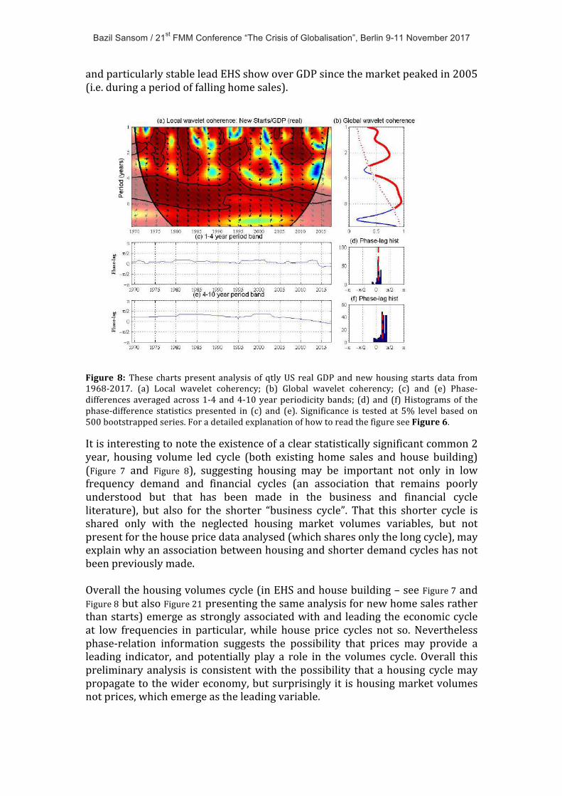
Figure 8:ThesechartspresentanalysisofqtlyUS realGDPandnewhousingstartsdata from1968-2017. (a) Local wavelet coherency; (b) Global wavelet coherency; (c) and (e) Phase-differencesaveragedacross1-4and4-10yearperiodicitybands; (d)and(f)Histogramsof thephase-difference statisticspresented in (c) and (e). Significance is tested at 5% level basedon500bootstrappedseries.ForadetailedexplanationofhowtoreadthefigureseeFigure6.
Itisinterestingtonotetheexistenceofaclearstatisticallysignificantcommon2year, housing volume led cycle (both existing home sales and house building)(Figure 7 and Figure 8), suggesting housing may be important not only in lowfrequency demand and financial cycles (an association that remains poorlyunderstood but that has been made in the business and financial cycleliterature), but also for the shorter “business cycle”. That this shorter cycle isshared only with the neglected housing market volumes variables, but notpresentforthehousepricedataanalysed(whichsharesonlythelongcycle),mayexplainwhyanassociationbetweenhousingandshorterdemandcycleshasnotbeenpreviouslymade.Overallthehousingvolumescycle(inEHSandhousebuilding–seeFigure7andFigure8butalsoFigure21presentingthesameanalysisfornewhomesalesratherthanstarts)emergeasstronglyassociatedwithandleadingtheeconomiccycleat low frequencies in particular,while house price cycles not so. Neverthelessphase-relation information suggests the possibility that prices may provide aleading indicator, andpotentially play a role in the volumes cycle.Overall thispreliminaryanalysis is consistentwith thepossibility thatahousingcyclemaypropagatetothewidereconomy,butsurprisinglyit ishousingmarketvolumesnotprices,whichemergeastheleadingvariable.

Bazil Sansom / 21st FMM Conference “The Crisis of Globalisation”, Berlin 9-11 November 2017
3.2 Networkdiscoveryand‘rootcause’analysisHaving identified a strong relationship and common cycle between housingvariables and GDP it would be interesting to better identify the transmissionfrom housing variables to aggregate demand as well as the relationshipsbetween housing variables. I also wish to consider financial variables aspotentialsourcesofcyclicalityorimportantmediatingvariablesinthehousing-macronexus.Inordertobegintounpacktheserelationships,Istudythehousingvariables house prices (HPI), and existing home sales (EHS) data, and privateresidential fixed investment (PRFI) and further decompose GDP into non-residentialinvestment(PNRFI)anddurable(Durables)andnon-durablepersonalconsumption expenditure (Non-durables) components. I study these detailedhousingandmacrovariablesalongsideimportantassociatedfinancialvariableshomemortgagecredit (M) andconsumercredit (CC) aswell asmortgagerates(Mi) and long-run rates (LTi). In all cases I study year on year change in thevariableunderstudyusingquarterlydataoverthesampleperiod1975-2017. Ifocus this analysis over the 4 to 10 year periodicity range overwhich I foundGDPcoherencewithhousingvariables(section3.1)exhibitsaclearspectralpeaksincethissignificantandtimepersistentcycleseemsakeyfeaturetoexplain.Inthis first iterationIdonotstudytheroughly2yearcycleapparentlysharedbyGDP andhousing volumes,which is left to a further iteration/extension of theinitialworkpresentedhere.Figure9presentstheresultsfromthe5%significancelevelthresholdedbivariateglobal coherenceweighted and phase-lag directed network resulting from theunconditional analysis (see methodology section 2.2). A number of strikingresultsemergefromthisinitialnetworkdiscoveryprocedure.Theimportantandleadingroleofthehousingmarketintheeconomiccycleisconfirmed,howeverand perhaps most strikingly, existing home sales (EHS) emerge as the key“source”node in thenetwork thus as a candidate ‘root cause’ of the economiccycle at this frequency.EHShave zero in-degree, and residential investment isledonlybytheexistinghomesalescycle(Figure10).Bothleadandarestronglyassociatedwithanumberofothervariablesinthenetwork.IndeedfromEHSitispossibletoreacheveryothernodeinthenetworkexceptforlongtermrates(which is theonlyothervariablewithzero in-degree,however from long termrates it is only possible to reach financial variableswith no path to aggregatedemand).ThisgivesEHSauniquepositioninthenetworkandimpliescyclesinEHS may propagate to all variables in the network (besides LTi). Meanwhilehousepricesemergeasasinknodefromwhichyoucanonlyreachfinancial(andnoreal)variables.Thisperhapscomesasasurprisegiventhegrowingliteratureidentifying house prices as a leading indicator, as well as on account of theimportant rolegiven to collateralvaluesandwealth inmacroeconomic theory;while housing market volumes have not been studied or theorised in themacroeconomic literature.Financialvariablesthemselvesemergeaspuresinks(with no path to aggregate demand). What is more credit quantities leadmortgage rates rather than the other way around (indeed mortgage ratesemerge–allbeitamongalimitedsetoffinancialvariables–asaglobalfinancialsink).

Bazil Sansom / 21st FMM Conference “The Crisis of Globalisation”, Berlin 9-11 November 2017
Figure9:Adirectededge(X−Y)signifiescoherencesignificantatthe95%confidencelevelwithX leadingY.Edges arephase-lag directed from lead to lag variable; edges areglobalcoherenceweighted; node size is proportional to out-degree; source nodes are coloured yellow and sinknodesarecoloureddarkgreen;nodesfromwhichyoucanonlyreachfinancialvariablesinksarecolouredpalegreen.RedarrowsandnodestraceapathfromtherealsourceEHStotherealsinkNon-durablesbyalwaysfollowingtheedgewiththesmallestphase-lagi.e.thispathdescribesthetemporal ordering between these variables. Analysis is based on year-on-year change forquarterlydatafromq11975toq22017(about40yearsofdata).Sincethebivariateglobalwaveletcoherenceemployedinestimatingtheseedgesisnotaconditionalstatistic, it isvery likelythatthesenon-trivial linkscapturebothdirectandindirectrelationshipsbetweenvariables.Whilethesephase-leadstatisticsarenotabletounpickindependentfromdependentlead/lags,theydoprovideacompletetemporalorderingbetweenthevariablesinthenetwork.Forexample starting from the source existing home sales (EHS) (from where asalreadynoteditispossibletoreachanyothernodeexceptlong-termrates)andfollowing the shortest phase-lead edge at each step (i.e. the nearest directneighbourinatemporalsense)generatesapathfromexistinghomesalestothelocal sink non-durable consumption that runs existing home sales→residentialinvestment→ durable consumption→ non-residential investment→ non-durableconsumption (this path is highlighted in red in Figure 9). While this temporalorderingdoesnotbyanymeansruleoutotherdirectlinks,itmaygiveindicateatransmissionchain.
Net.1:USeconomy1975-2017Globalwaveletcoherenceweightedphasedirectednetwork-4-10yearperiodband

Bazil Sansom / 21st FMM Conference “The Crisis of Globalisation”, Berlin 9-11 November 2017
Figure10:ThishighlightsimportantaspectsofthetopologyofthenetworkpresentedinFigure9.Yellowarrowsindicateout-edgesandgreenarrowsindicatein-edges.WeseethatEHShasazero in-degree, and that the only incoming edge received by residential investment is fromexistinghomesales.Overall the results of the initial network discovery exercise seems to raisequestionsregardingtheprecedencegiventohousepricesandfinancialvariablesin the wider macroeconomic literature; confirm the importance of housebuildingidentifiedbyasmallexistingliterature;andsuggesttheinterestingandunexpectedpossibilitythatacycleinsecondaryhousingmarketvolumesdrivestheaggregatedemandcycle.Althoughthepossibilitythatthephase-leadexistingsales have over residential investment may represent a faster response byexisting home sales compared to residential investment to some omittedcommon driver must also be considered. Either way the important questionarisesofwhyhousingmarketsalesvolumescycle.Thismaybetheresultoftwo-way causalitywithother variables, somethingnot capturedbyphase-directionwhichisbydefinitionuni-directional.
3.3 DetailedconditionalstudyofEHSlinkstodemandvariablesWhilenetwork1(Figure9)isalreadyinformative,itwouldbeveryhelpfulifwewereabletodisentangleindependentvs.dependent(ordirectvs.indirect)edgesinthisgraph.ForexampleEHSisPRI’sonlyincomingedge,whatismoresincehousesalesvolumesarewidelyreadintherealestateindustryasakeyindicatorofmarketdemand,itseemsrelativelyeasytoimaginethathousebuildingmightfollow a cycle in existing home sales; however is there a direct channel fromexisting home sales to non-residential investment? Or is this non-trivial linkmediated by residential investment and/or durable consumption etc.? Partialcoherenceandphase-lagstatisticsprovideatoolwithwhichwemaybeabletogain some further insight into these questions by helping us to unpickindependent from dependent or direct from indirect edges in the networkpresentedinFigure9.

Bazil Sansom / 21st FMM Conference “The Crisis of Globalisation”, Berlin 9-11 November 2017
Unpickingdirectvs.indirectchannelsfromEHStoGDP
Figure 11: The graph resulting from network-discovery process in (Figure 9) suggestsstatistically significant coherence between existing home sales (EHS) and all four aggregatedemandcomponentsincludedintheanalysis(durableandnon-durableconsumption(Durables,Non-Durables), residential and non-residential investment (PRFI, PNRFI)) with EHS leadingdemandvariables.Thegraphalso suggests thepossibilityhowever, that someof thesemaybeindirectoratleasthaveindirectcomponents.ForexamplewhilstEHSistheonlyleadingedgeforPRFI, both EHS and PRFI lead and exhibit significant coherencewith durables. This raises thequestion whether EHS have any direct impact on durable consumption, or whether thisrelationshipismostlymediatedbyhousinginvestmentetc.Sinceexistinghomesalesemergefrommynetworkdiscoveryprocedureasthekeysourcevariableandpotential“rootcause”ofaggregatedemandcyclesatlowfrequenciesinnetwork1,IwillfocusmyfurtheranalysisonthelinksfromEHSto demand variables. I will therefore look at the coherence and phaserelationship for all edges between existing home sales and demand variables,comparing bivariate and partial results. For the partial analysis I will, morespecifically,lookateachoftheseedgesconditionalonthepotentialindirectlinkssuggested by the topology of network 1 as presented in Figure 9 (this idea isillustrated in Figure 11). Partial wavelet coherence and phase-differenceconditional on other incoming edges should provide some insight into whichdemandcomponentsaredirectly,andwhichonlyindirectlyimpactedbyhousingtransactions in order to try and achieve more detailed insight into thetransmissionpathfromhousingtowiderdemand.
(a) (b)
(d)(c)
Bazil Sansom / 21st FMM Conference “The Crisis of Globalisation”, Berlin 9-11 November 2017
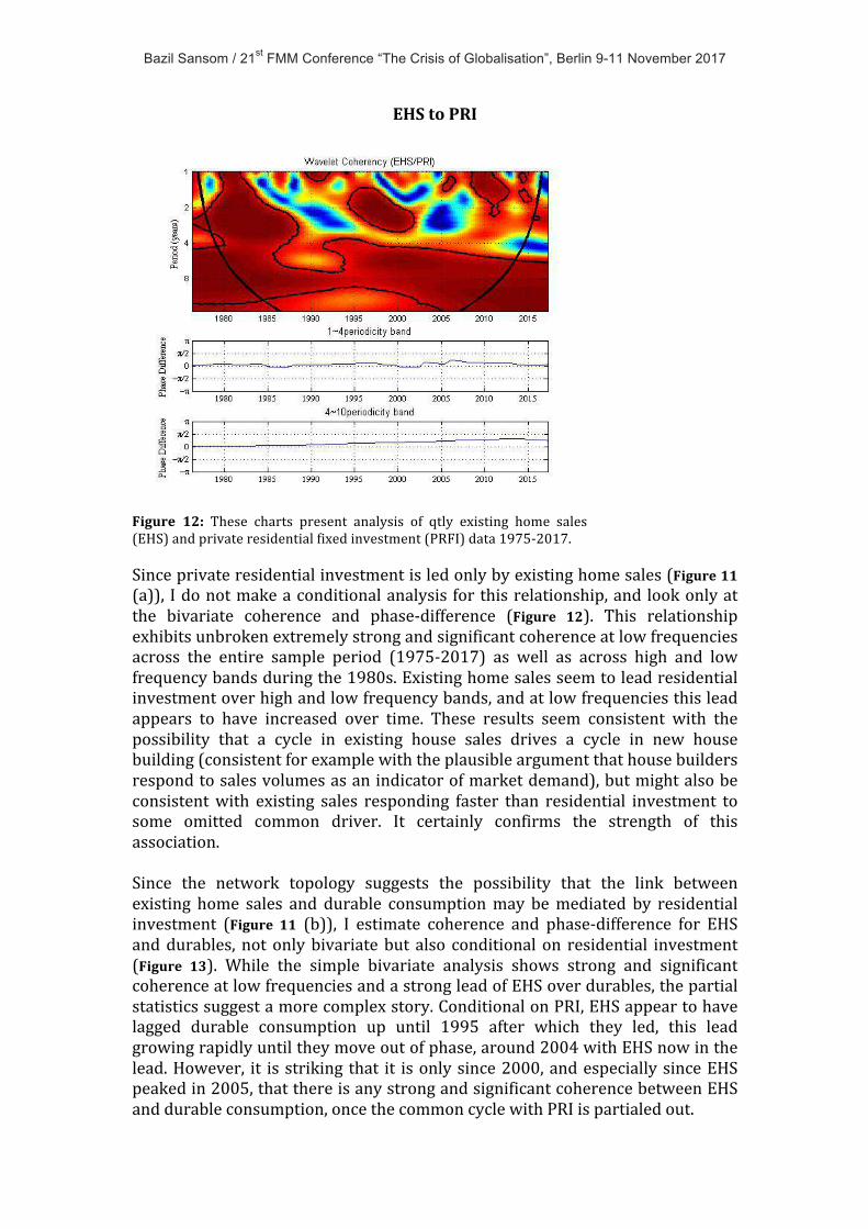
EHStoPRI
Figure 12: These charts present analysis of qtly existing home sales(EHS)andprivateresidentialfixedinvestment(PRFI)data1975-2017.Sinceprivateresidentialinvestmentisledonlybyexistinghomesales(Figure11(a)), Idonotmakeaconditionalanalysis forthisrelationship,and lookonlyatthe bivariate coherence and phase-difference (Figure 12). This relationshipexhibitsunbrokenextremelystrongandsignificantcoherenceatlowfrequenciesacross the entire sample period (1975-2017) as well as across high and lowfrequencybandsduringthe1980s.Existinghomesalesseemtoleadresidentialinvestmentoverhighandlowfrequencybands,andatlowfrequenciesthisleadappears to have increased over time. These results seem consistent with thepossibility that a cycle in existing house sales drives a cycle in new housebuilding(consistentforexamplewiththeplausibleargumentthathousebuildersrespondtosalesvolumesasanindicatorofmarketdemand),butmightalsobeconsistentwith existing sales responding faster than residential investment tosome omitted common driver. It certainly confirms the strength of thisassociation.Since the network topology suggests the possibility that the link betweenexisting home sales and durable consumptionmay bemediated by residentialinvestment (Figure 11 (b)), I estimate coherence and phase-difference for EHSanddurables, notonlybivariatebut also conditionalon residential investment(Figure 13). While the simple bivariate analysis shows strong and significantcoherenceatlowfrequenciesandastrongleadofEHSoverdurables,thepartialstatisticssuggestamorecomplexstory.ConditionalonPRI,EHSappeartohavelagged durable consumption up until 1995 after which they led, this leadgrowingrapidlyuntiltheymoveoutofphase,around2004withEHSnowinthelead.However, it isstriking that it isonlysince2000,andespeciallysinceEHSpeakedin2005,thatthereisanystrongandsignificantcoherencebetweenEHSanddurableconsumption,oncethecommoncyclewithPRIispartialedout.

Bazil Sansom / 21st FMM Conference “The Crisis of Globalisation”, Berlin 9-11 November 2017
EHStoDurableConsumption
Figure 13: These charts present analysis of qtly existing home sales (EHS) and durableconsumption(Durables)data1975-2017.Thelefthandpanelpresentsbivariateanalysis,andtheright hand panel partial analysis conditional on private residential fixed investment (PRI) –durableconsumption’sonlyotherleadingedge(Figure9andseeFigure11(b)).Seefiguresin3.1.2forhowtointerpretthegraphs.Since the network topology suggests the possibility that the link betweenexisting home sales and non-residential investmentmay bemediated by bothresidential investment and durables (Figure 11 (c)), I estimate coherence andphase-differenceforEHSandnon-residentialinvestment,notonlybivariatebutalso conditional on residential investment and durables (Figure 14). Significantcoherence shows up in this relationship from the 1990s with EHS leadingstrongly suggesting an important role for housing in this investment cycle,however this coherence seems to be eliminated in the conditional casesuggestingthe impactofEHSonnon-residential investmentmaybeprincipallyoperatingviaresidentialinvestmentanddurableconsumption15.
15While partial coherence at low frequencies seems mostly weak, partial phase lag shifts fromstronglyleadingtostronglylaggingupto1995,afterwhichEHSleadnon-residentialinvestment.ThismaysimplyreflectthestrongaccelerationinEHS.Howeverwehadbetterfocusourphaseanalysisonareasofsignificantcoherence.

Bazil Sansom / 21st FMM Conference “The Crisis of Globalisation”, Berlin 9-11 November 2017
EHStoPNRI
Figure14:Bivariateandpartialwaveletcoherenceandphase-differenceforexistinghomesales(EHS)andprivatenon-residentialfixedinvestment(PNRFI).Partialstatisticsareconditionalonprivateresidentialfixedinvestment(PRFI)anddurableconsumption(Durables)–PNRFI’sothertwoleadingedgesinthenetworkrepresentedinFigure9(seeFigure11(c)).The much weaker coherence between existing home sales and non-durableconsumption, since non-durable consumption is a local sink variable, ispotentiallymediatedby a number of other variables (Figure 11 (d)). I estimatecoherenceandphase-differenceforEHSandnon-durableconsumption,notonlybivariate but also conditional on non-residential investment (non-durableconsumptions only other significant incoming edge) (Figure 15). While someareas of strong coherence show up - specifically from 2000 - and EHS leadconsumption strongly in the bivariate analysis, lower frequency coherenceseems to be substantially eliminated when studied conditional on non-residential investment suggesting that for low frequencies at least, thisrelationship is indirect and operating via non-residential investment, itselfdrivenbyresidentialinvestmentanddurablescycles16.16Interestinglysomeareasofsignificantcoherencedoshowupathigherfrequencies.

Bazil Sansom / 21st FMM Conference “The Crisis of Globalisation”, Berlin 9-11 November 2017
EHStoNon-durables
Figure15:Bivariateandpartialwaveletcoherenceandphase-differenceforexistinghomesales(EHS)andnon-durableconsumption(Non-Durables).Partialstatisticsareconditionalonprivatenon-residential fixed investment - non-durables consumptions only other edge in the networkrepresentedinFigure9.(seeFigure11(d)).Overall a very significant and consistent relationship between existing homesales and residential investment is identified. There is also evidence of a non-trivial linkdirectpath frommarketvolumestodurableconsumptionoperatingindependently of residential investment. While there is strong and significantcoherence between housing market volumes and non-residential investmentovertheentirepost1995period,partialanalysissuggeststhisrelationshipmaybe largely indirect and substantially mediated by residential investment anddurable consumption patterns. Similarly the relationship between housingmarket volumes and non-durable consumption seems to bemediated by non-residential investment, itself driven by residential investment and durableconsumption.

Bazil Sansom / 21st FMM Conference “The Crisis of Globalisation”, Berlin 9-11 November 2017
4 DiscussionandconclusionWhileoverallthisdatadrivenempiricalworkbroadlyconfirmstheincreasinglyrecognised importance of housing cycles in the business cycle, a number ofstriking and novel results emerge. The importancewidely attributed to housepricesinexistingmacroeconomicliteraturesisnotsupported,withhousepricesemergingasa ‘sink’variablenota ‘source’, laggingbothaggregatedemandandother housing variables. Meanwhile the importance and leading character ofhousebuildingcyclespreviously identified inasmallexisting literature isverymuchconfirmedwithresidentialinvestmentshowinghighcoherencewithandatemporal lead over other demand components. However the analysis alsounexpectedly identifies non-trivial low frequency cycles in existinghome sales(secondary housingmarket volumes) as leading residential investment cycles.Existinghomesalesthusemergeasthemostleadingvariable.Sincehousesalesvolumesarewidelyregardedasanimportantindicatorofmarketdemandintherealestateindustry,itseemsentirelyplausiblethatacycleinexistinghomesalescouldtransmittohousebuilding,althoughthepossibilitythatthephase-leadofEHSoverresidentialinvestmentcouldrepresentafasterresponsetosomethirdcommondriveromitted frommyanalysismustalsobe considered.Eitherwaythe question of why secondary housing market volumes cycle emerges as animportantissue.Partialanalysissuggestsnon-trivialtransmissionfromexistinghomesalevolumescyclesnotonlytoresidentialinvestmentbutalsodirectlytodurable consumption, with residential investment and durable consumptioncycles transmitting to non-residential investment, and this “business cycle” innon-residential investment, further transmitting in turn to wider non-durableconsumption.Thepossibilitythusemergesthatalowfrequencycycleinhousingmarket volumes (a variable and a cycle unstudied in the macroeconomicliterature),propagatesthroughtheeconomy,andistherootcauseofnon-trivialcyclesinaggregatedemand.Furtherworkisrequiredtotestandinterprettheseresults,buttheyseemtosuggestthebasisforanalternativeandnoveltheoryoflong-run economic cycles and beg further empirical and theoretical effort.Further research might: consider a larger set of variables; take a moreunsupervisedandsystematicapproachtodeployingpartialanalysisfornetworkthinning (and cleaning out indirect edges); also apply bi-directional directedstatistics touncover thecausal structureof thenetwork;pursueempiricalandtheoretical work on both why home sales cycle, as well as on studying andexplainingthelinksbetweenhomesalesanddurablesandhousebuilding(sincethese appear to be themost important and direct links). Perhaps some of themost obvious questions emerging from this study are: (1) What is the linkbetween existing home sales and residential investment? (2)What is the linkbetweenexistinghomesalesanddurable consumption?Butalsoandcrucially,(3) Why do existing home sales volumes cycle? Seriously addressing thesequestionsisoutsideofthescopeofthisparticularstudyandsomethingItakeupinfurtherworkandpapers.
Bazil Sansom / 21st FMM Conference “The Crisis of Globalisation”, Berlin 9-11 November 2017
AcknowledgementsIamhappyandgratefultobenefittingfromcodeforwaveletsanalysisdevelopedandmadeavailablebyA.GrinstedandbyMaria JoanaSoaresand LuísAguiar-Conraria (available at below referenced web-links) to which I have referredextensivelyandfromwhichIhavebenefitedfromverymuchindevelopingtheanalysis here presented. My thanks also to Engelbert Stockhammer and toRobertJumpfordiscussionandinterest.Grinsted: https://uk.mathworks.com/matlabcentral/fileexchange/47985-cross-wavelet-and-wavelet-coherenceAguiar-Conrria and Soares: https://sites.google.com/site/aguiarconraria/-joanasoares-waveletsReferencesAdalid,Ramon,andCarstenDetken.2007.LiquidityShocksandAssetBoom/bust
Cycles.Aguiar-Conraria,Luís,andMariaJoanaSoares.2014.“TheContinuousWavelet
Transform:MovingbeyondUniandBivariateAnalysis.”JournalofEconomicSurveys28(2):344–75.
Alessi,Luciaetal.2014.“ComparingDifferentEarlyWarningSystems:ResultsfromaHorseRaceCompetitionamongMembersoftheMacro-PrudentialResearchNetwork.”1–27.
Alessi,Lucia,andCarstenDetken.2009.“RealTime”EarlyWarningIndicatorsforCostlyAssetPriceBoom/BustCycles:ARoleforGlobalLiquidity.
Álvarez,LuisJ.,andAlbertoCabrero.2010.DoesHousingReallyLeadtheBusinessCycle?
Barbosa-filho,NelsonH.,CodrinaRadaVonArnim,LanceTaylor,andLucaZamparelli.2008.“CyclesandTrendsinU.S.NetBorrowingFlows.”JournalofPostKeynesianEconomics30(4):623–48.
Bauer,Margretetal.2007.“ChemicalProcessUsingTransferEntropy.”15(1):12–21.
Bezemer,Dirk,andLuZhang.2014.“FromBoomtoBustintheCreditCycle:TheRoleofMortgageCredit.”
Blasius,Bernd,AmitHuppert,andLewiStone.1999.“ComplexDynamicsandPhaseSynchronizationinSpatiallyExtendedEcologicalSystems.”Nature399(May):354–59.
Borio,Claudio.2014.“TheFinancialCycleandMacroeconomics:WhatHaveWeLearnt?”JournalofBankingandFinance45:182–98.
Borio,Claudio,andMathiasDrehmann.2009.“AssessingtheRiskofBankingCrises–Revisited.”BISQuarterlyReview(March):29–46.
Borio,Claudio,andPhilipLowe.2002.AssetPrices,FinancialandMonetaryStability:ExploringtheNexus.
Burns,ArthurF.,andWesleyC.Mitchell.1946.“MeasuringBusinessCycles.”inStudiesinBusinessCyclesno.2.NewYork:NBER.
Büyükkarabacak,B.,andN.T.Valev.2010.“TheRoleofHouseholdandBusinessCreditinBankingCrises.”JournalofBanking&Finance34(6):1247–56.
Cazelles,Bernard,MarioChavez,GuillaumeConstantinDeMagny,SimonHales,andJean-francoisGue.2007.“Time-DependentSpectralAnalysisof
Bazil Sansom / 21st FMM Conference “The Crisis of Globalisation”, Berlin 9-11 November 2017
EpidemiologicalTime-SerieswithWavelets.”JournaloftheRoyalSociety,Interface4:625–36.
Chatfield,C.1989.TheAnalysisofTimeSeries.editedbyHallandChapman.Claessens,Stijn,AyhanM.Kose,MarcoE.Terrones,andIMF.2012.“What
HappensDuringRecessions,CrunchesandBusts?”EconomicPolicy60:653–700.
Crowe,Christopher,GiovanniDellAriccia,DenizIgan,andPauRabanal.2013.“HowtoDealwithRealEstateBooms:LessonsfromCountryExperiences.”JournalofFinancialStability9(3):300–319.
Damos,Petros.2016.“UsingMultivariateCrossCorrelations,GrangerCausalityandGraphicalModelstoQuantifySpatiotemporalSynchronizationandCausalitybetweenPestPopulations.”BMCEcology1–17.
Daubechies,I.1990.“TheWaveletTransformTime-FrequencyLocalizationandSignalAnalysis.”IEEETransactionsonInformationTheory36:961–1004.
Daubechies,Ingrid.1992.TenLecturesonWavelets.Philadelphia,USA:SIAM.Davis,E.Philip,andHaibinZhu.2004.BankLendingandCommercialProperty
Cycles:SomeCross-CountryEvidence.Davis,Morris,andJonathanHeathcote.2005.“HousingandtheBusinessCycle.”
InternationalEconomicReview46:751–84.Detto,Matteoetal.2013.“MultivariateConditionalGrangerCausalityAnalysis
forLaggedResponseofSoilRespirationinaTemperateForest.”4266–84.Dufrénot,Gilles,andSheheryarMalik.2012.“TheChangingRoleofHousePrice
DynamicsovertheBusinessCycle.”EconomicModelling29(5):1960–67.Ferrara,Laurent,andOlivierVigna.2009.CyclicalRelationshipsbetweenGDPand
HousingMarketinFrance:FactsandFactorsatPlay.Gabor,D.1946.“TheoryofCommunication.”JournalInstituteElectricalEngineers
93:429–457.Goodhart,Charles,andBorisHofmann.2008.HousePrices,Money,Creditandthe
Macroeconomy.Goupillaud,P.,A.Grossmann,andJ.Morlet.1984.“CycleOctaveandRelated
TransformsinSeismicSignalAnalysis.”Geoexploration23:85–102.Grinsted,A.,J.C.Moore,andS.Jevrejeva.2004.“ApplicationoftheCrossWavelet
TransformandWaveletCoherencetoGeophysicalTimeSeries.”NonlinearProcessesinGeophysics11:561–66.
Hudgins,L.,C.Friehe,andM.Mayer.1993.“WaveletTransformsandAtmosphericTurbulence.”PhysicsReviewLetters71:3279–3282.
Igan,Deniz,AlainKabundi,FranciscoNadal,DeSimone,andMarceloPinheiro.2011.“Housing,Credit,andRealActivityCycles:CharacteristicsandComovement.”JournalofHousingEconomics20(3):210–31.
IMF.2008.“TheChangingHousingCycleandtheImplicationsforMonetaryPolicy.”Pp.103–32inWorldEconomicOutlook:HousingandtheBusinessCycle.
IMF.2012.WorldEconomicOutlook,Chapter3.IMF,DenizIgan,A.Kabundi,andNdSimone.2009.ThreeCycles:Housing,Credit,
andRealActivity.IMF,DanielLeigh,DenizIgan,JohnSimon,andPetiaTopalova.2012.“Dealing
WithHouseholdDebt.”Pp.1–36inIMFWorldEconomicOutlook.Jorda,Oscar,MoritzSchularick,andAlanM.Taylor.2012.“WhenCreditBites
Back:Leverage,BusinessCycles,andCrises.”FederalReserveBankofSanFranciscoWorkingPaperSeries(October):1–42.

Bazil Sansom / 21st FMM Conference “The Crisis of Globalisation”, Berlin 9-11 November 2017
Jorda,Oscar,MoritzSchularick,andAlanM.Taylor.2014.TheGreatMortgaging :HousingFinance,Crises,andBusinessCycles.
Juselius,Mikael,andMathiasDrehmann.2015.“LeverageDynamicsandtheRealBurdenofDebt.”(501).
Kindleberger,C.,andR.Aliber.2005.Manias,Panics&Crashes:AHistoryofFinancialCrises.editedbyNJHoboken.Wiley.
King,Mervyn.1994.“DebtDeflation:TheoryandEvidence.”EuropeanEconomicReview38:419–45.
Kuramoto,Yoshiki.1984.ChemicalOscillations,Waves,andTurbulence.Berlin:Springer.
Kydland,FinnE.,PeterRupert,andRomanSustek.2016.“HousingDynamicsovertheBusinessCycle.”InternationalEconomicReview57(4):1149–78.
Leamer,E.E.2007.HousingIstheBusinessCycle.Long,ClarenceJr.1940.BuildingCyclesandtheTheoryofInvestment.Princeton
andLondon:PrincetonUniversityPressandOxfordUniversityPress.Mallat,S.G.1999.AWaveletTourofSignalProcessing.AcademicPress.Mian,Atif,AmirSufi,andEmilVerner.2015.“HouseholdDebtandBusiness
CyclesWorldwide.”NBERWorkingPapers(609).Mormann,Florian,KlausLehnertz,PeterDavid,andChristianE.Elger.2000.
“MeanPhaseCoherenceasaMeasureforPhaseSynchronizationandItsApplicationtotheEEGofEpilepsyPatients.”144:358–69.
Ng,EricK.W.,andJohnnyC.L.Chan.2012.“GeophysicalApplicationsofPartialWaveletCoherenceandMultipleWaveletCoherence.”JournalofAtmosphericandOceanicTechnology29:1845–53.
Nolte,Guidoetal.2008.“RobustlyEstimatingtheFlowDirectionofInformationinComplexPhysicalSystems.”PhysicalReviewLetters100.
Pikovsky,A.S.,M.G.Rosenblum,andJ.Kurths.2001.Synchronization:AUniversalConceptinNonlinearSciences.Cambridge,UK:CambridgeUniversityPress.
Reinhart,CarmenM.,andKennethS.Rogoff.2011.ThisTimeIsDifferent.PrincetonUniversityPress.
Rosenblum,MichaelG.,ArkadyS.Pikovsky,andJürgenKurths.1996.“PhaseSynchronizationofChaoticOscillators.”PhysicalReviewLetters76(11):1804–7.
Rosenblum,Michael,ArkadyPikovsky,JurgenKurths,CarstenSchafer,andPeterA.Tass.2001.“PhaseSynchronization:FromTheorytoDataAnalysis.”Pp.279–321inHandbookofBiologicalPhysics,Vol.4,Neuro-informatics,editedbyFMossandSGielen.
Schularick,Moritz,andAlanM.Taylor.2009.CreditBoomsGoneBust:MonetaryPolicy,LeverageCyclesandFinancialCrises,1870-2008.
Schulte,JustinA.,RaymondG.Najjar,andMingLi.2016.“JournalofHydrology:RegionalStudiesTheInfluenceofClimateModesonStreamflowintheMid-AtlanticRegionoftheUnitedStates.”JournalofHydrology:RegionalStudies5:80–99.
Shao,Pei-chiangetal.2015.“GrangerCausality-BasedSynapticWeightsEstimationforAnalyzingNeuronalNetworks.”JournalofComputationalNeuroscience38(3):483–97.
Soares,MariaJoana,andLuísAguiar-Conraria.2011.TheContinuousWaveletTransform:APrimer.
Szemere,Robert,MichelaScatigna,andKostasTsatsaronis.2014.“ResidentialPropertyPriceStatisticsacrosstheGlobe.”BISQuarterlyReview

Bazil Sansom / 21st FMM Conference “The Crisis of Globalisation”, Berlin 9-11 November 2017
(September):61–76.Torrence,Christopher,andGilbertP.Compo.1998.“APracticalGuidetoWavelet
Analysis.”BulletinoftheAmericanMeteorologicalSociety79:61–78.Williamson,MarkS.,SebastianBathiany,andTimothyM.Lenton.2016.“Early
WarningSignalsofTippingPointsinPeriodicallyForcedSystems.”EarthSystemDynamics7:313–26.
Yuan,Tao,andS.JoeQin.2014.“RootCauseDiagnosisofPlant-WideOscillationsUsingGrangerCausality.”JournalofProcessControl24(2):450–59.
Zhang,Wenjun.2011.“ConstructingEcologicalInteractionNetworksbyCorrelationAnalysis:HintsfromCommunitySampling.”NetworkBiology1(2):81–98.
Zou,Cunlu,ChristopheLadroue,ShuixiaGuo,andJianfengFeng.2010.“IdentifyingInteractionsintheTimeandFrequencyDomainsinLocalandGlobalNetworks-AGrangerCausalityApproach.”Bioinformatics11(337).
5 Appendix
5.1 WaveletsFigure16:Morletwavelet
Figure17:Waveletspowerspectrumplot
Source:(SoaresandAguiar-Conraria2011)

Bazil Sansom / 21st FMM Conference “The Crisis of Globalisation”, Berlin 9-11 November 2017
Figure18:Phase-differencecircle
5.2 DatadefinitionsandsourcesVariable Description SourceExistingHomeSales(EHS)
Numberofunits.Existing-homesalesarebasedonclosingtransactionsofsingle-family,town-homes,condominiumsandcooperativehomes.
NationalAssociationofRealtors(ReleaseExistingHomeSales).
NewHomeSales(NHS)
U.S.BureauoftheCensus(Release:NewResidentialSales).
Newhousingstarts
Totalnewprivatelyownedhousingunitsstarted.
U.S.BureauoftheCensus(Release:NewResidentialConstruction).
Housepriceindex(HPI)
All-TransactionsHousePriceIndexfortheUnitedStates.Estimatedusingsalespricesandappraisaldata.
U.S.FederalHousingFinanceAgency(Release:HousePriceIndex).
Housepriceindex(HPI)
Nationalsources,BISResidentialPropertyPricedatabase.
Long-termrates(LTi)
Long-terminterestratesrefertogovernmentbondsmaturingintenyears.Ratesareimpliedbypriceatwhichbondstraded.
OECDLong-terminterestrates,US.
Mortgagerates(Mi)
30-YearFixedRateMortgageAverageintheUnitedStates.
FreddieMac(Release:PrimaryMortgageMarketSurvey).
Mortgagedebt(M)
HouseholdsandNonprofitOrganizations;HomeMortgages;Liability,Level.
BoardofGovernorsoftheFederalReserveSystem(US).(Release:Z.1FinancialAccountsoftheUnitedStates.SeriesIDLA153165105.Q.)
Privateresidentialfixedinvestment(PRFI)
U.S.BureauofEconomicAnalysis,GrossDomesticProduct(BEAAccountCode:A011RC1).
Privatenon-residentialfixedinvestment(PNRFI)
Privateinvestment,fixed,non-residential.
U.S.BureauofEconomicAnalysis,GrossDomesticProduct(BEAAccountCode:A008RC1).
Durableconsumption
Personalconsumptionexpenditure–durables.
U.S.BureauofEconomicAnalysis,GrossDomesticProduct(BEAAccountCode:DDURRC1).
Non-durableconsumption
Personalconsumptionexpenditure–non-durables.
U.S.BureauofEconomicAnalysis,GrossDomesticProduct(BEAAccountCode:DNDGRC1).

Bazil Sansom / 21st FMM Conference “The Crisis of Globalisation”, Berlin 9-11 November 2017
5.3 Powerspectrums
Figure19:USrealGDPpowerspectrum
Note:ThisfigurepresentsatheGWPSforUSrealGDPdataoveralongerperiodreflectingthegreateravailabilityofGDPdatacomparedtohousingvariables.
Figure20:USNewHousingStartspowerspectrum
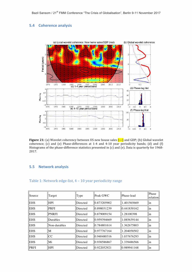
Bazil Sansom / 21st FMM Conference “The Crisis of Globalisation”, Berlin 9-11 November 2017
5.4 Coherenceanalysis
Figure21:(a)WaveletcoherencybetweenUSnewhousesales(---)andGDP;(b)Globalwaveletcoherence; (c) and (e) Phase-differences at 1-4 and 4-10 year periodicity bands; (d) and (f)Histogramsofthephase-differencestatisticspresentedin(c)and(e).Dataisquarterlyfor1968-2017.
5.5 NetworkanalysisTable1:Networkedge-list,4–10yearperiodicityrange
Source Target Type Peak GWC Phase-lead Phase
relation
EHS HPI Directed 0.873205902 1.401565669 in
EHS PRFI Directed 0.898031239 0.441830162 in
EHS PNRFI Directed 0.879009154 1.28100398 in
EHS Durables Directed 0.959394669 1.085639144 in
EHS Non-durables Directed 0.784801614 1.362675803 in
EHS M Directed 0.977767164 1.204058502 in
EHS CC Directed 0.940480316 1.037676293 in
EHS Mi Directed 0.938586867 1.339486566 in
PRFI HPI Directed 0.922052921 0.989941168 in

Bazil Sansom / 21st FMM Conference “The Crisis of Globalisation”, Berlin 9-11 November 2017
PNRFI HPI Directed 0.881762747 0.269187647 in
Durables HPI Directed 0.802529079 0.243031644 in
HPI M Directed 0.809207365 0.406619204 in
LTi HPI Directed 0.849120169 0.031356293 in
HPI Mi Directed 0.869811429 0.032906525 in
PRFI PNRFI Directed 0.892822884 1.044605769 in
PRFI Durables Directed 0.936727032 0.473606137 in
PRFI M Directed 0.893836158 1.269327101 in
PRFI CC Directed 0.82545729 1.014315502 in
Durables PNRFI Directed 0.877448732 0.638334436 in
PNRFI Non-durables Directed 0.857667064 0.489254184 in
PNRFI CC Directed 0.751198973 0.347969466 in
PNRFI Mi Directed 0.856307984 0.315884131 in
Durables M Directed 0.960152905 0.844338328 in
Durables CC Directed 0.974649014 0.9838477 in
CC M Directed 0.929305634 0.562106848 in
M Mi Directed 0.850688775 0.758749918 in
CC Mi Directed 0.86308292 0.242247131 in
5.6 Periodicitybandselection
Localpeakclusters:3clusters
Figure22:Clustersbasedonk-means.Threecentroidshaveperiodicityof9,5.5and3yearsleadingtoperiodicitybandsplitsof1-4.2,4.2-7.3and7.3to10.Thisk=3clusteringproducesstableresult,wherek=2unstable.