Progress In Electromagnetics Research, Vol. 112, 155–181, 2011

RAINFALL RATE PROBABILITY DENSITY EVALUA-TION AND MAPPING FOR THE ESTIMATION OF RAINATTENUATION IN SOUTH AFRICA AND SURROUND-ING ISLANDS

P. A. Owolawi

Department of Electrical EngineeringMangosuthu University of TechnologyUmlazi, KwaZulu-Natal, South Africa

Abstract—The paper describes the modelling of the average rainfallrate distribution measured at different locations in South Africa.There are three major aspects this paper addresses: to develop arainfall rate model based on the maximum likelihood method (ML);to develop contour maps based on rainfall rate at 0.01% percentage ofexceedence; and re-classification of the ITU-R and Crane rain zonesfor the Southern Africa region. The work presented is based on five-minute rainfall data converted to one-minute equivalent using a newlyproposed hybrid method. The results are mapped and comparedwith conventional models such as the ITU-R model, Rice-Holmberg,Moupfouma and Crane models. The proposed rainfall rate modelsare compared and evaluated using root mean square and chi-square(χ2) statistics. Then re-classification of the rain zone using ITU-R andCrane designations is suggested for easy integration with existing radioplanning tools. The rainfall rate contour maps at 0.01% percentage ofexceedence are then developed for South Africa and its surroundingislands.

1. INTRODUCTION

Signal transmission at microwave and millimeter bands providesseveral advantages over lower frequency bands which include extensivebandwidth, frequency re-use, small antenna as well as short timedeployment. The propagation of waves in this frequency range ispredominantly by line-of-sight propagation and thus, there are certain

Received 25 August 2010, Accepted 26 November 2010, Scheduled 11 January 2011Corresponding author: Pius Adewale Owolawi (owolani@mut.ac.za).

156 Owolawi

phenomena which affect the signal strength at these bands. Themost important factor to take into consideration at these bands is theattenuation and scattering due to rain [1]. The simplest approach toemploy in estimating rain attenuation is to use measured rainfall ratestatistics where applicable. If this is not available, modeled rainfall ratestatistics for a specified geographic region should be considered [2].

In fact, a lot of research has been conducted in the area of rainfallrate modeling, and expressions to determine rainfall rate value atgiven percentages of exceedence has been proposed. The most widelyknown models are Crane’s Global Climatic Model [3], the ITU-R P-837recommendation [4], originally developed under CCIR in 1974 and nowin its fifth revision under ITU-R. Other rainfall rate distribution modelscommonly referred to by many workers in this field are Rice-Holmberg’smodel [5], Moupfouma et al. model [6], and Ajayi and Ofoche model[7]. In the Southern Africa, similar research has been conducted byOwolawi et al., Fashuyi et al., and Mulangu et al. [8–14]. The workdone and reported by Seeber [15] for South Africa and the surroundingislands of Marion and Gough was based on 15-minute integration time.This approach is not very suitable for system planners because thehigh integration time used may not respond to rapid changes in thecumulative distribution of rainfall rate.

The works done in [11, 12] are based on rainfall rate integrationtime conversion factors of a location in South Africa and as stated inthe papers, the results were generalized for other stations. In the recentwork submitted [16], a hybrid method was proposed for the conversionof rain rate from 5-minute integration time to 1-minute equivalent;which involves regional parameters that influence the rainfall ratedistribution curves.

1.1. Review of Existing Rain Rate Models

Rain rate modelling is an important component used in the estimationof rain attenuation and thus, the fade margins for a specifiedgeographical region. The models are often classified into two classeswhich are: global and localized rain rate models.

In global rain rate models, the mechanism used primarily dependson climatic parameters and geographical locations. There are severalglobal rain rate models available but for the purpose of this paper, thetwo models considered are two are Crane’s and ITU-R global models.

The work done by Crane [3] classified the globe into eight regions;each labelled A through H with varying degrees of dryness to wetness.The ITU-R provides another global rain rate climatic model termedcharacteristics of precipitation for propagation modelling. The model

Progress In Electromagnetics Research, Vol. 112, 2011 157

was originally developed under CCIR in 1974 and several revisions havebeen made from ITU-R P837-1 to recently revised ITU-R P.837-5 [4].

Although both Crane and ITU-R global climatic models are widelyknown and adopted by many telecommunication companies to plantheir link budget, they may not be adequate to account for seasonal andyearly variation. This dynamic variation of rainfall is not uncommonin South Africa’s climatic zones as confirmed by other researchers intheir localities. In the comparison carried out with the previous ITU-R recommendations [17], South America’s tropical zone was confirmedto have a large area, the Crane’s global model classified it as zone H,thus it has 209.7 mm/hr rain rate at 0.01% percentage of exceedence [3];while the ITU-R recognised the zone as three different rain zones of80mm/hr, 100 mm/hr and 120mm/hr. This means that the differencebetween the rain rates estimated by the two models is about 100%.

In many sites in South Africa and surrounding Islands, a similartrend of large variation is observed. In Durban, the ITU-R P.837-1 mapped rain rate to be 22 mm/hr at 0.01%, the ITU-R P.837-5 suggested 50 mm/hr while Crane represented the rain rate by46.8mm/hr. The trend of variation between P.837-1 to P.837-5 is about39% difference. The percentage difference between P.837-1 and Crane’ssuggested rain rate is 36%. In the enforce ITU-R P.837-5 the differencebetween ITU-R and Crane is 3.3% for Durban. This latter result showsa better improvement in the ITU-R global climatic rain rate model.In summary, the prime advantage of global rain rate is that even inthe absence of lofty spatial resolution of point rain rate information,estimation of rain rate can be determined at a given percentage ofexceedence using universal climatic information to characterize eachof the regions of the globe. The limitations of the previous ITU-Rrecommendations such as discontinuity is taken care off in the enforcerecommendation but the effects of cyclic year, variability and seasonalchanges are still issues to be rectified.

In the case of local rain rate models, researchers from differentparts of the world have proposed several regional based rainfall ratemodels. These rain rate models are developed from empirical equationsusing results of field measurements collected over a long period ofyears. Rain rate climatic models in this category which deserves tobe mentioned include Rice-Holmberg model [5], Dutton-Dougherty-Martin model [20], Crane two-component model [3], Moupfouma-Martin model [6], and Seeber rain rate model [15].

158 Owolawi

2. EXPERIMENTAL MEASUREMENT FACILITIES

The rainfall data employed in this study has been collected by twodifferent rain measuring equipment. Measurements have been obtainedby means of Oregon Rain gauge and Joss-Waldvogel Distrometer(JWD). In addition, over ten years rainfall data with five-minuteintegration time has been provided by the South Africa WeatherService (SAWS).

An Oregon rain gauge (RGR 382) was installed at the Latitude(30◦58’E) and Longitude (29◦52’S) with an altitude of 139.7 metersat the School of Electrical, Electronics and Computer Engineeringin the University of KwaZulu-Natal, Howard College campus. Therain gauge collector has a diameter measuring 101.6 mm, and stands146.05mm high. The gauge contains a collecting bucket that tipsafter accumulation of 1mm of rainfall. The measuring accuracy of thebucket with rain rate of 0–15mm per hour is +/ − 10% while above15mm per hour is +/ − 15%. The gauge functioned for a period ofone-year (2005–2006).

The Joss-Waldvogel distrometer is an instrument for measuringraindrop size distribution (DSD). This equipment is not limited tomeasuring raindrop distribution only, but is also incorporated intoprecipitation field measurement purposely to validate and complementthe measurements of the rain gauge. The distrometer used in thisstudy is capable of measuring rain rate, reflectivity, rain accumulation,raindrop size (diameter range 0.3–5.5mm) at 60-second intervals withan accuracy of 5%. For the current study, the distrometer was installedin December 2008, and commenced operation in January 2009 with asampling interval integrated over one minute. Both the rain gauge andJoss-Waldvogel distrometer are present at the master site (control site)and located approximately 2 meters from each other. The site is freeof noise and shielded from abnormal winds.

Finally, the South Africa Weather Services (SAWS) providesrainfall data of five-minute integration time for over ten years for allthe provinces in South Africa and the surrounding Islands. SAWSuse different means to collect their precipitation data. The mostwidely used method is via a network of rain gauges. Rain gaugesused by SAWS are standard 127 mm in accordance with the WorldMeteorological Organization (WMO) standard. The 127 mm is thediameter of the rimmed circular funnel opening. The other type ofrain gauge used by SAWS is the automated rain gauge, which is atipping bucket rain gauge with a 200 mm funnel opening. The dataused in this study is based on the specification and calibration of thetwo types of rain gauges mentioned. In the case of distrometer, 92%

Progress In Electromagnetics Research, Vol. 112, 2011 159

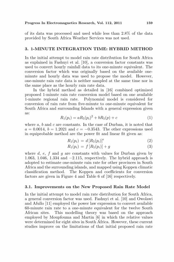
of its data was processed and used while less than 2.8% of the dataprovided by South Africa Weather Services was not used.

3. 1-MINUTE INTEGRATION TIME: HYBRID METHOD

In the initial attempt to model rain rate distribution for South Africaas explained in Fashuyi et al. [10], a conversion factor constants wasused to convert hourly rainfall data to its one-minute equivalent. Theconversion factor which was originally based on the available one-minute and hourly data was used to propose the model. However,one-minute rain rate data is neither sampled at the same time nor inthe same place as the hourly rain rate data.

In the hybrid method as detailed in [16] combined optimizedproposed 1-minute rain rate conversion model based on one available1-minute regional rain rate. Polynomial model is considered forconversion of rain rate from five-minute to one-minute equivalent forSouth Africa and surrounding Islands with a general expression givenas:

R1(pi) = aR5(pi)2 + bR5(p) + c (1)

where a, b and c are constants. In the case of Durban, it is noted thata = 0.0014, b = 1.2021 and c = −0.3543. The other expressions usedin equiprobable method are the power fit and linear fit given as:

R1(pi) = d [R5(pi)]e (2)R1(pi) = f [R5(pi)] + g (3)

where d, e, f and g are constants with values for Durban given by1.063, 1.046, 1.334 and −2.115, respectively. The hybrid approach isadopted to estimate one-minute rain rate for other provinces in SouthAfrica and the surrounding islands, and mapped using Koppen climaticclassification method. The Koppen and coefficients for conversionfactors are given in Figure 4 and Table 6 of [16] respectively.

3.1. Improvements on the New Proposed Rain Rate Model

In the initial attempt to model rain rate distribution for South Africa,a general conversion factor was used. Fashuyi et al. [10] and Owolawiand Afullo [11] employed the power law expression to convert available60-minute rain rate to a one-minute equivalent for the twelve SouthAfrican sites. This modelling theory was based on the approachemployed by Moupfouma and Martin [6] in which the relative valueswere determined for eight sites in South Africa. However, these currentstudies improve on the limitations of that initial proposed rain rate

160 Owolawi

model which may not be adequate in describing the rain rate due tothe following reasons:

• Lack of one-minute rain rate to carry out conversion processesusing power laws for the entire country and surrounding islands;

• Unavailability of long term rain data to develop the model thattakes care of cyclic years;

• Fitting of the rain rate data with other established rain ratemodels may lead to the concession of the model parameters.

In this new proposed approach, all these factors are taken intoconsideration and are properly and adequately addressed. The currentproposal uses a maximum likelihood estimator to fit different statisticaldistributions. The work presented is based on more than ten yearsfive-minute rainfall data converted to a one-minute equivalent using anewly developed hybrid model.

In addition to the ten years rainfall data, the other parametersemployed in this work are average annual total rainfall M (mm/yr), thehighest monthly precipitation Mm (mm/month), the average numberof thunderstorm day in a year (Dth) day which are extracted fromWorld Meteorological organization documents 1953 and 1962 [18, 19]and estimated ratio of convective rain or thunderstorm to the totalaverage rainfall accumulation (β) as expressed in Dutton et al. [20].

3.2. Performance of the Proposed Conversion Method

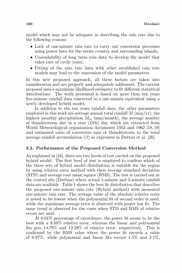
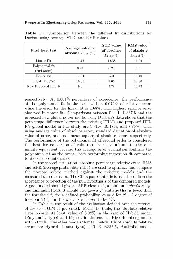
As explained in [16], there are two levels of test carried on the proposedhybrid model. The first level of test is employed to confirm which ofthe three sets of hybrid model distribution is suitable for the regionby using relative error method with their average standard deviation(STD) and average root mean square (RMS). The test is carried out atthe control site (Durban) where actual 1-minute and 5-minute rainfalldata are available. Table 1 shows the best fit distribution that describesthe proposed one-minute rain rate (Hybrid method) with measuredone-minute rain rate. The average value of the absolute relative erroris noted to be lowest when the polynomial fit of second order is used,while the maximum average error is observed with power law fit. Thesame trend is observed for the cases when STD and RMS of relativeerrors are used.

At 0.01% percentage of exceedence, the power fit seems to be thebest with a 9.88% relative error, whereas the linear and polynomialfits give 14.79% and 12.28% of relative error, respectively. This isconfirmed by the RMS value where the power fit records a valueof 0.97%, while polynomial and linear fits record 1.5% and 2.1%,

Progress In Electromagnetics Research, Vol. 112, 2011 161

Table 1. Comparison between the different fit distributions forDurban using average, STD, and RMS values.

First level testAverage value of

absolute ERel,i(%)

STD value

of absolute

ERel,i(%)

RMS value

of absolute

ERel,i(%)

Linear Fit 11.72 12.38 16.69

Polynomial fit

(2nd order)6.74 6.21 9.0

Power Fit 14.64 5.0 15.40

ITU-R P.837-5 10.85 7.05 12.80

New Proposed ITU-R 9.0 4.78 10.72

respectively. At 0.001% percentage of exceedence, the performanceof the polynomial fit is the best with a 0.072% of relative error,while the error for the linear fit is 1.68%, with highest relative errorobserved in power fit. Comparisons between ITU-R P.837-5 and theproposed new global power model using Durban’s data shows that thepercentage difference between the existing ITU-R and proposed ITU-R’s global model in this study are 9.31%, 19.18%, and 8.85%, whenusing average value of absolute error, standard deviation of absolutevalue of error, and root mean square of absolute error, respectively.The performance of the polynomial fit of second order is consideredthe best for conversion of rain rate from five-minute to the one-minute equivalent because the average error evaluation confirms thepolynomial fit as the overall best performing regression fit comparedto its other counterparts.

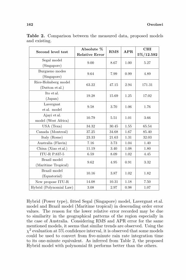
In the second evaluation, absolute percentage relative error, RMSand APR (average probability ratio) are used to optimize and comparethe propose hybrid method against the existing models and themeasured rain rate data. The Chi-square statistic is used to confirm theacceptance or rejection of the null hypothesis of the compared models.A good model should give an APR close to 1, a minimum absolute ε(p)and minimum RMS. It should also give a χ2 statistic that is lower thanthe threshold tδ for a defined probability value δ for N − 1 degree offreedom (DF). In this work, δ is chosen to be 5%.

In Table 2, the result of the evaluation defined over the intervalof 1% to 0.001% is presented. From the table, the absolute relativeerror records its least value of 3.08% in the case of Hybrid model(Polynomial type) and highest in the case of Rice-Holmberg modelwith 63.22%. The other models that fall below 10% of absolute relativeerrors are Hybrid (Linear type), ITU-R P.837-5, Australia model,

162 Owolawi

Table 2. Comparison between the measured data, proposed modelsand existing.

Second level testAbsolute %

Relative ErrorRMS APR

CHI

5%/12.592

Segal model

(Singapore)9.00 8.67 1.00 5.27

Burgueno modes

(Singapore)9.64 7.99 0.99 4.89

Rice-Holmberg model

(Dutton et al.)63.22 47.15 2.94 171.31

Ito et al.

(Japan)19.28 15.69 1.25 17.02

Lavergnat

et al. model9.58 3.70 1.06 1.76

Ajayi et al.

model (West Africa)10.79 5.51 1.01 3.66

USA (Texa) 34.32 30.45 1.55 65.54

Canada (Montreal) 37.25 34.68 1.67 85.40

Italy (Rome) 23.33 21.63 1.31 32.03

Australia (Flavin) 7.16 3.73 1.04 1.40

China (Xiao et al.) 11.19 3.40 1.08 1.80

ITU-R P.837-5 6.59 8.09 1.02 4.45

Brazil model

(Maritime Tropical)9.62 4.95 0.91 3.32

Brazil model

(Equatorial)10.16 3.87 1.02 1.82

New propose ITU-R 14.08 10.31 1.18 7.50

Hybrid (Polynomial Law) 3.08 2.97 0.98 1.07

Hybrid (Power type), fitted Segal (Singapore) model, Lavergnat et al.model and Brazil model (Maritime tropical) in descending order errorvalues. The reason for the lower relative error recorded may be dueto similarity in the geographical patterns of the region especially inthe case of Australia. Considering RMS and APR error for the samementioned models, it seems that similar trends are observed. Using theχ2 evaluation at 5% confidence interval, it is observed that some modelscould be used to convert from five-minute rain rate integration timeto its one-minute equivalent. As inferred from Table 2, the proposedHybrid model with polynomial fit performs better than the others.

Progress In Electromagnetics Research, Vol. 112, 2011 163

4. PROBABILITY THEORY OF THE PROPOSED RAINRATE MODEL

Since it may be impossible to provide rainfall data for the prediction ofattenuation due to rain at any instant in future, a probabilistic model isthen required for system designer for both terrestrial and satellite linkdesigns. In this section, three distribution models with their maximumlikelihood estimators are presented. The preferred distributions areWeibull, Lognormal and Gamma, which are widely used to describeprecipitation distribution pattern over a defined period. They aredescribed as follow:

I. Two parameters Weibull distribution: the probability density of 1-minute rain rate at a give probability of exceedence R1(p) mm/hris given as [21]:

f(R1(p))=

{αβ

(R1β

)α−1exp

[−

(R1β

)α], R1(p) ≥, α ., β . 0

0 elsewhere

}(4)

and the distribution is given as:

F (R1(p)) =

{1− exp

[−

(R1β

)α], R1(p) ≥, α ., β . 0

0 elsewhere

}(5)

where α.0 is the shape parameter and β.0 is the scale parameter.Suppose that rain rate R1(p) is observation at different percentageof exceedence which is denoted by p1, p2, p3, . . . pN . The likelihoodfunction may be given as

ln L = N ln α−Nα ln β+(α−1)N∑

i=1

lnR(pi)−N∑

i=1

(R(pi)

β

)α

(6)

The maximum likelihood estimate of parameters α̂ and β̂ assumedsolution at condition when:

∂ ln L

∂α= 0 (7)

∂ ln L

∂β= 0 (8)

N denotes sample size and the Newton-Raphson approximationmethod is used to solve simultaneous equations at the rth iterativeby the expression:

α̂(r) = α(r − 1) + h(r)

β̂(r) = β(r − 1) + k(r)(9)

164 Owolawi

where h(r) and k(r) are the correction terms given in theEquation (10) [21, 22]:

[hk

]=

[∂2 ln L∂α2

∂2 ln L∂α∂β

∂2 ln L∂β∂α

∂2 ln L∂β2

]−1 [−∂ ln L

∂α

−∂ ln L∂β

](10)

In this work, the iteration is terminated at the point of convergencewhere the correction terms lies below approximately 0.002. Thederivation to all first order and second order derivatives arepresented in the Appendix A of [21].

II. Two parameters lognormal distribution: the lognormal with twoparameters, µ and σ represent location and scale parameters,respectively. The probability density of 1-minute rain rate ata given probability of exceedence R1(p)mm/hr as expressed byEvans et al. [23] and Walack [24] as:

f(R1(p)) =exp

(−1

2

(ln R1(p)−µ

σ

)2)

xσ√

2π0 ≤ R1(p) < +∞ (11)

where σ = scale parameter of the included normal distribution(σ > 0), µ = location parameter of the included normaldistribution.Here, the maximum likelihood estimation for the two-parameterlognormal used is given by Eckhard et al. [25] and Suhaila andJemain [26] as:

µ̂ = exp

(1n

N∑

i=1

log R(pi)

)=

(N∏

i=1

R(pi)

) 1N

(12)

σ̂ = exp

∣∣∣∣∣∣

(1

N − 1

N∑

i=1

[log

(R(pi)

µ̂

)]2) 1

2

∣∣∣∣∣∣(13)

The mean (µ) of rain rate data R1(p) and the standard deviation(σ) are calculated. The µ̂ and σ̂ are then estimated usingthe expressions µ/

√ω and exp(

√log(ω), respectively, with ω =

1 + (σ/µ)2 = 1 + CV 2. [Note CV is called coefficient of variationwith the expression given as CV = (exp(σ2)− 1)0.5].

III. Two parameters Gamma distribution: two parameters gammadistribution probability density function for rain rate R1(p) isgiven as [23]:

f(R1(p)) =1

βγΓ(γ)R1(p)γ−1 exp(−R1(p)/β), γ, β . 0, R1(p) . 0

(14)

Progress In Electromagnetics Research, Vol. 112, 2011 165

where γ and β are the shape and scale parameters, respectivelyand Γ is denote gamma function. Considering a given data set ofrain rate R1(p), maximum likelihood estimates of γ and β can beestimated by solving the following equations by Thom [27], theapproximate expression to estimate γ̂ is given as:

γ̂ =1 + (1 + 4A/3)0.5

4A(15)

β̂ = Nγ̂/N∑

i=1

R1(pi) (16)

where A = log x̄− (N∑

i=1log R1(pi))/N .

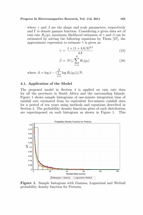
4.1. Application of the Model

The proposed model in Section 4 is applied on rain rate datafor all the provinces in South Africa and the surrounding Islands.Figure 1 shows sample histograms of one-minute integration time ofrainfall rate estimated from its equivalent five-minute rainfall datafor a period of ten years using methods and equations described inSection 4. The probability density functions plots of each distributionare superimposed on each histogram as shown in Figure 1. This

Probability Density Function for Pretoria

Histogram Gamma Lognormal Weibull

Rainfall Rate (mm/hr)

100806040200

pd

f

0.8

0.72

0.64

0.56

0.48

0.4

0.32

0.24

0.16

0.08

0

Figure 1. Sample histogram with Gamma, Lognormal and Weibullprobability density function for Pretoria.

166 Owolawi

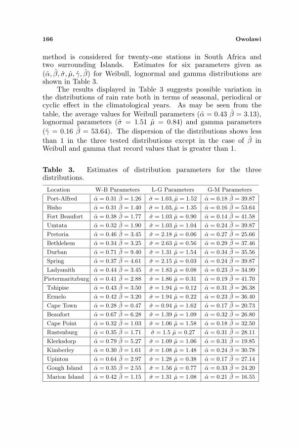
method is considered for twenty-one stations in South Africa andtwo surrounding Islands. Estimates for six parameters given as(α̂, β̂, σ̂, µ̂, γ̂, β̂) for Weibull, lognormal and gamma distributions areshown in Table 3.

The results displayed in Table 3 suggests possible variation inthe distributions of rain rate both in terms of seasonal, periodical orcyclic effect in the climatological years. As may be seen from thetable, the average values for Weibull parameters (α̂ = 0.43 β̂ = 3.13),lognormal parameters (σ̂ = 1.51 µ̂ = 0.84) and gamma parameters(γ̂ = 0.16 β̂ = 53.64). The dispersion of the distributions shows lessthan 1 in the three tested distributions except in the case of β̂ inWeibull and gamma that record values that is greater than 1.

Table 3. Estimates of distribution parameters for the threedistributions.

Location W-B Parameters L-G Parameters G-M Parameters

Port-Alfred α̂ = 0.31 β̂ = 1.26 σ̂ = 1.03, µ̂ = 1.52 α̂ = 0.18 β̂ = 39.87

Bisho α̂ = 0.31 β̂ = 1.40 σ̂ = 1.03, µ̂ = 1.35 α̂ = 0.16 β̂ = 53.64

Fort Beaufort α̂ = 0.38 β̂ = 1.77 σ̂ = 1.03 µ̂ = 0.90 α̂ = 0.14 β̂ = 41.58

Umtata α̂ = 0.32 β̂ = 1.90 σ̂ = 1.03 µ̂ = 1.04 α̂ = 0.24 β̂ = 39.87

Pretoria α̂ = 0.46 β̂ = 3.45 σ̂ = 2.18 µ̂ = 0.06 α̂ = 0.27 β̂ = 25.66

Bethlehem α̂ = 0.34 β̂ = 3.25 σ̂ = 2.63 µ̂ = 0.56 α̂ = 0.29 β̂ = 37.46

Durban α̂ = 0.71 β̂ = 9.40 σ̂ = 1.31 µ̂ = 1.54 α̂ = 0.34 β̂ = 35.56

Spring α̂ = 0.37 β̂ = 4.61 σ̂ = 2.15 µ̂ = 0.03 α̂ = 0.24 β̂ = 39.87

Ladysmith α̂ = 0.44 β̂ = 3.45 σ̂ = 1.83 µ̂ = 0.08 α̂ = 0.23 β̂ = 34.99

Pietermaritzburg α̂ = 0.41 β̂ = 2.88 σ̂ = 1.86 µ̂ = 0.31 α̂ = 0.19 β̂ = 41.70

Tshipise α̂ = 0.43 β̂ = 3.50 σ̂ = 1.94 µ̂ = 0.12 α̂ = 0.31 β̂ = 26.38

Ermelo α̂ = 0.42 β̂ = 3.20 σ̂ = 1.94 µ̂ = 0.22 α̂ = 0.23 β̂ = 36.40

Cape Town α̂ = 0.28 β̂ = 0.47 σ̂ = 0.94 µ̂ = 1.62 α̂ = 0.17 β̂ = 20.73

Beaufort α̂ = 0.67 β̂ = 6.28 σ̂ = 1.39 µ̂ = 1.09 α̂ = 0.32 β̂ = 26.80

Cape Point α̂ = 0.32 β̂ = 1.03 σ̂ = 1.06 µ̂ = 1.58 α̂ = 0.18 β̂ = 32.50

Rustenburg α̂ = 0.35 β̂ = 1.71 σ̂ = 1.5 µ̂ = 0.27 α̂ = 0.31 β̂ = 28.11

Klerksdorp α̂ = 0.79 β̂ = 5.27 σ̂ = 1.09 µ̂ = 1.06 α̂ = 0.31 β̂ = 19.85

Kimberley α̂ = 0.30 β̂ = 1.61 σ̂ = 1.08 µ̂ = 1.48 α̂ = 0.24 β̂ = 30.78

Upinton α̂ = 0.64 β̂ = 2.97 σ̂ = 1.28 µ̂ = 0.38 α̂ = 0.17 β̂ = 27.14

Gough Island α̂ = 0.35 β̂ = 2.55 σ̂ = 1.56 µ̂ = 0.77 α̂ = 0.33 β̂ = 24.20

Marion Island α̂ = 0.42 β̂ = 1.15 σ̂ = 1.31 µ̂ = 1.08 α̂ = 0.21 β̂ = 16.55

Progress In Electromagnetics Research, Vol. 112, 2011 167

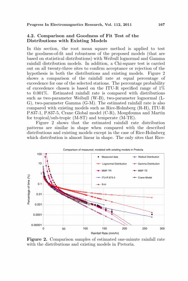
4.2. Comparison and Goodness of Fit Test of theDistributions with Existing Models

In this section, the root mean square method is applied to testthe goodness-of-fit and robustness of the proposed models (that arebased on statistical distributions) with Weibull lognormal and Gammarainfall distribution models. In addition, a Chi-square test is carriedout on all twenty-three sites to confirm acceptance or rejection of thehypothesis in both the distributions and existing models. Figure 2shows a comparison of the rainfall rate at equal percentage ofexceedence for one of the selected stations. The percentage probabilityof exceedence chosen is based on the ITU-R specified range of 1%to 0.001%. Estimated rainfall rate is compared with distributionssuch as two-parameter Weibull (W-B), two-parameter lognormal (L-G), two-parameter Gamma (G-M). The estimated rainfall rate is alsocompared with existing models such as Rice-Holmberg (R-H), ITU-RP.837-1, P.837-5, Crane Global model (C-R), Moupfouma and Martinfor tropical/sub-tropic (M-ST) and temperate (M-TE).

Figure 2 shows that the estimated rainfall rate distributionpatterns are similar in shape when compared with the describeddistributions and existing models except in the case of Rice-Holmbergwhich distribution is almost linear in shape. The only sites that Rice-

Comparison of measured, modeled with existing models in Pretoria

0.00001

0.0001

0.001

0.01

0.1

1

10

100

0 100 150 200 250 300

Rainfall Rate (mm/hr)

Pe

rce

nta

ge

of

tim

e (

%)

Measured data Weibull Distribution

Lognormal Distribution Gamma Distribution

MMF-TR MMF-TE

ITU-R 873-5 Crane Model

R-H

50

Figure 2. Comparison samples of estimated one-minute rainfall ratewith the distributions and existing models in Pretoria.

168 Owolawi

Holmberg distribution describes properly are Gough Island, MarionIsland, Upington and Klerksdop. ITU-R recommendations P.837-1and P.837-2 give the same pattern distribution of estimated rainfallbut does not properly fit into the data (especially that of ITU-RP.837-1). The ITU-R P.837-5, that is currently in-force, gives a betterdescription of sites such as Pretoria, Ermelo, Cape Town, and the othertwo Islands. These mentioned locations may be sampled sites for ITU-R as well as Crane Global for extrapolation of rain climatic zones forSouth Africa and the surrounding Islands. In this work, both Weibulland Gamma distributions show a better description of the estimatedrainfall rate distribution for the majority of the selected sites; the Cranedistribution model shows reasonably acceptable distribution in somesites such as Pretoria and Cape Town.

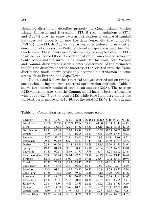
Tables 4 and 5 show the statistical analysis carried out on twenty-one stations using the two statistical optimization methods. Table 4shows the numeric results of root mean square (RMS). The averageRMS values indicates that the Gamma model has the best performancewith about 4.23% of the total RMS, while Rice-Holmberg model hasthe least performance with 19.36% of the total RMS. W-B, M-TE, and

Table 4. Comparison using root mean square error.

Location W-B L-G G-M R-H ITU-R 1 ITU-R 5 C-R M-ST M-TE

Port-Alfred 8.366 16.273 11.239 17.04 53.83 44.00 38.78 11.43 6.13

Bisho 13.11 35.18 12.29 14.62 64.60 55.15 41.72 33.18 13.85

Fort Beaufort 14.54 42.48 13.09 15.89 34.71 40.38 37.23 20.07 10.57

Umtata 8.49 40.68 7.42 16.05 38.52 43.35 33.09 14.34 9.72

Pretoria 5.47 57.47 7.54 33.06 27.31 6.92 8.88 7.86 9.71

Bethlehem 29.80 92.62 8.60 45.80 61.49 15.11 46.99 11.69 32.77

Durban 22.34 64.50 10.14 85.26 54.28 34.85 29.30 11.31 24.04

Spring 19.33 81.49 11.76 88.98 15.96 40.64 16.22 16.22 13.81

Ladysmith 11.40 60.11 13.05 68.77 45.78 15.47 15.58 12.02 23.44

Pietermaritzburg 22.89 36.74 24.64 27.28 59.96 40.49 33.96 19.40 14.64

Tshipise 12.11 57.06 5.09 48.35 17.26 23.51 17.42 15.07 10.93

Ermelo 12.92 73.19 12.83 78.45 47.31 8.55 47.31 11.32 21.11

Cape Town 15.54 13.46 2.30 56.02 18.27 2.59 2.89 9.71 2.79

Beaufort 9.43 61.11 14.85 53.56 26.42 8.38 11.29 13.30 7.56

Cape Point 11.26 13.45 2.85 69.52 33.48 16.12 18.29 8.55 14.27

Rustenburg 11.93 48.67 2.58 50.63 32.50 16.89 20.09 7.44 14.05

Klerksdorp 17.32 6.15 5.14 20.01 18.38 28.87 6.20 15.06 7.71

Kimberley 22.84 5.0 4.83 73.59 32.13 16.72 19.82 17.33 9.60

Upinton 23.75 14.89 7.42 18.20 21.20 26.32 9.71 17.28 20.88

Gough Island 3.39 5.13 3.48 6.31 17.40 7.27 13.33 6.73 7.96

Marion Island 13.06 48.24 14.10 4.69 39.32 7.24 36.46 14.61 4.65

Progress In Electromagnetics Research, Vol. 112, 2011 169

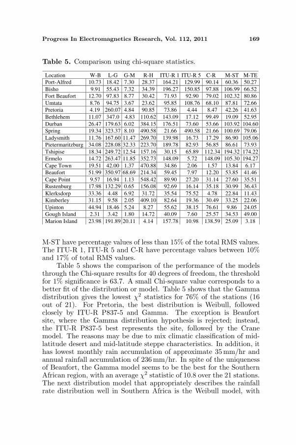
Table 5. Comparison using chi-square statistics.

Location W-B L-G G-M R-H ITU-R 1 ITU-R 5 C-R M-ST M-TE

Port-Alfred 10.73 18.42 7.30 28.37 164.21 129.99 90.14 60.36 50.27

Bisho 9.91 55.43 7.32 34.39 196.27 150.85 97.88 106.99 66.52

Fort Beaufort 12.70 97.83 8.77 30.42 71.93 92.90 79.02 102.32 80.86

Umtata 8.76 94.75 3.67 23.62 95.85 108.76 68.10 87.81 72.66

Pretoria 4.19 260.07 4.84 90.85 73.86 4.44 8.47 42.26 41.63

Bethlehem 11.07 347.0 4.83 110.62 143.09 17.12 99.49 19.09 52.95

Durban 26.47 179.63 6.02 384.15 176.51 73.60 53.66 103.92 104.60

Spring 19.34 323.37 8.10 490.58 21.66 490.58 21.66 100.69 79.06

Ladysmith 11.76 167.60 11.47 269.70 139.98 16.73 17.29 86.90 105.06

Pietermaritzburg 34.08 228.08 32.33 223.70 189.78 82.93 56.85 86.61 73.93

Tshipise 18.34 249.72 12.54 157.16 30.15 65.89 112.34 194.32 174.22

Ermelo 14.72 263.47 11.85 352.73 148.09 5.72 148.09 105.30 194.27

Cape Town 19.51 42.00 1.37 470.88 34.86 2.06 1.57 13.84 6.17

Beaufort 51.99 350.97 68.69 214.34 59.45 7.97 12.20 53.85 41.46

Cape Point 9.57 16.94 1.13 548.42 89.90 27.20 31.14 27.60 35.51

Rustenburg 17.98 132.29 0.65 156.08 92.69 16.14 35.18 30.99 36.43

Klerksdorp 33.36 4.48 6.92 31.72 35.54 75.52 4.78 22.84 11.43

Kimberley 31.15 9.58 2.05 409.10 82.64 19.36 30.49 33.25 22.06

Upinton 44.94 18.46 5.24 8.27 55.62 38.15 76.61 9.86 24.05

Gough Island 2.31 3.42 1.80 14.72 40.09 7.60 25.57 34.53 49.00

Marion Island 23.98 191.89 20.11 4.14 157.78 10.98 138.59 25.09 3.18

M-ST have percentage values of less than 15% of the total RMS values.The ITU-R 1, ITU-R 5 and C-R have percentage values between 10%and 17% of total RMS values.

Table 5 shows the comparison of the performance of the modelsthrough the Chi-square results for 40 degrees of freedom, the thresholdfor 1% significance is 63.7. A small Chi-square value corresponds to abetter fit of the distribution or model. Table 5 shows that the Gammadistribution gives the lowest χ2 statistics for 76% of the stations (16out of 21). For Pretoria, the best distribution is Weibull, followedclosely by ITU-R P837-5 and Gamma. The exception is Beaufortsite, where the Gamma distribution hypothesis is rejected; instead,the ITU-R P837-5 best represents the site, followed by the Cranemodel. The reasons may be due to mix climatic classification of mid-latitude desert and mid-latitude steppe characteristics. In addition, ithas lowest monthly rain accumulation of approximate 35 mm/hr andannual rainfall accumulation of 236 mm/hr. In spite of the uniquenessof Beaufort, the Gamma model seems to be the best for the SouthernAfrican region, with an average χ2 statistic of 10.8 over the 21 stations.The next distribution model that appropriately describes the rainfallrate distribution well in Southern Africa is the Weibull model, with

170 Owolawi

an average χ2 statistic of 19.85. The other models give average χ2

statistics of above 55, which is rather too close to the threshold of63.7. Although they fall under acceptable threshold of the Chi-square,they may be least considered to describe rainfall rate distributions forthe Southern Africa.

5. RAINFALL RATE RE-ZONING FOR SOUTH AFRICAAND SURROUNDING ISLANDS

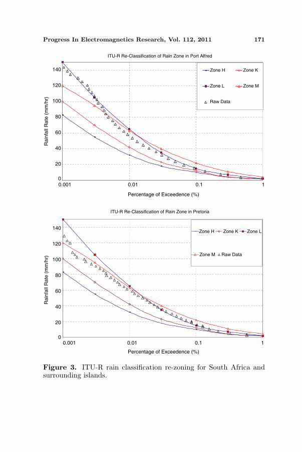
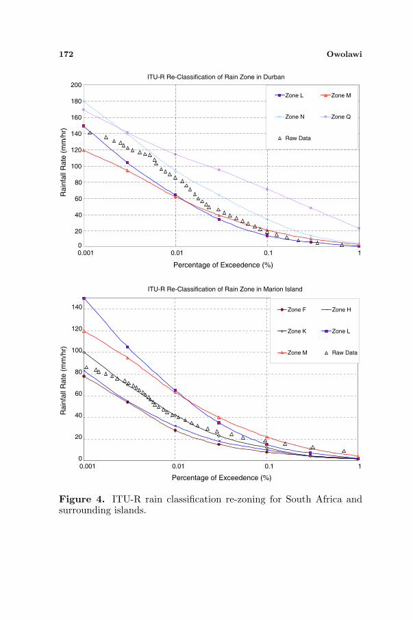
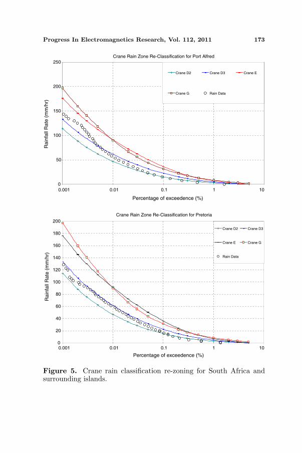
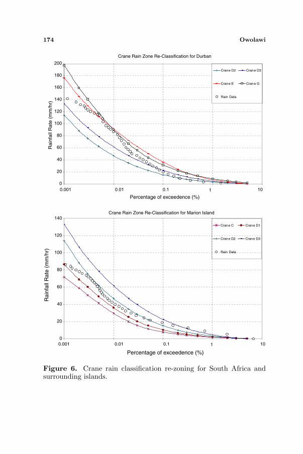
As rain rate becomes the principal component in determining rainattenuation when planning terrestrial and satellite links at higherfrequency. It may be a time-consuming process to evaluate a largenumber of sites [17]. The use of ITU-R and Crane’s designationsmay be of advantage over other models because many radio andsatellite planning tools are designed around these two major types ofdesignations. Since one of the applications of this paper is to provideinformation regarding rain rate distribution to system designers andradio design tools developers, it will be of advantage to adapt theregional re-zoning using the existing designations of ITU-R and Crane.Majority of researchers often conclude that ITU-R model either over-estimates or under-estimates the rainfall rate at a certain definedpercentage of exceedence. Figures 3 and 4 compare the rainfallrate distributions with ITU-R rain climate zone designations whileFigures 5 and 6 show the Crane’s climatic rain zones for differentsites in South Africa and its surrounding islands. Here the closestdesignation distribution to the measured data is chosen.

5.1. Comparative Studies of both ITU-R and Crane RainRate Zones

The reclassification is based on the chi-square optimization method.In Figure 3, Port Alfred shows that the currently enforced ITU-RP837-5 differs from the ITU-R P837-1 by 29.62%. The newly assigneddesignation of rain zone L with chi-square statistic of 7.16 at sixdegrees of freedom and at 5% confidence level differs from ITU-RP837-5 by 26.31%. Its counterpart, the Crane rain zone, as shownin Figure 5 considered D2 as the appropriate zone for the region anddiffers from the old designation of C by 22.67%. For the same degreesof freedom, the chi-square test confirmed Crane’s D1 and ITU-R L rainclimatic zones for Bisho with 13.65% and 9.09% differences from theold designations respectively. Pietermaritzburg and most of the studiedsites showed that ITU-R and Crane’s rain climatic zone under-estimaterainfall rate at 0.01% except in the case of Tshipise and Kimberley

Progress In Electromagnetics Research, Vol. 112, 2011 171

ITU-R Re-Classification of Rain Zone in Port Alfred

0

20

40

60

80

100

120

140

0.001 0.01 0.1 1

Percentage of Exceedence (%)

Rain

fall

Rate

(m

m/h

r)

Zone H Zone K

Zone L Zone M

Raw Data

ITU-R Re-Classification of Rain Zone in Pretoria

0.001 0.01 0.1 1

Percentage of Exceedence (%)

0

20

40

60

80

100

120

140

Rain

fall

Rate

(m

m/h

r)

Zone H Zone K Zone L

Zone M Raw Data

Figure 3. ITU-R rain classification re-zoning for South Africa andsurrounding islands.

172 Owolawi

ITU-R Re-Classification of Rain Zone in Durban

0

20

40

60

80

100

120

140

160

180

200

0.001 0.01 0.1 1

Percentage of Exceedence (%)

Rain

fall

Rate

(m

m/h

r)

Zone L Zone M

Zone N Zone Q

Raw Data

ITU-R Re-Classification of Rain Zone in Marion Island

Percentage of Exceedence (%)

Rain

fall

Rate

(m

m/h

r)

Zone F Zone H

Zone K Zone L

Zone M Raw Data

0.001 0.01 0.1 10

20

40

60

80

100

120

140

Figure 4. ITU-R rain classification re-zoning for South Africa andsurrounding islands.

Progress In Electromagnetics Research, Vol. 112, 2011 173

Crane Rain Zone Re-Classification for Port Alfred

0

50

100

150

200

250

0.001 0.01 0.1 1 10

Percentage of exceedence (%)

Rain

fall

Rate

(m

m/h

r)

Crane D2 Crane D3 Crane E

Crane G Rain Data

Crane Rain Zone Re-Classification for Pretoria

0

20

40

60

80

100

120

140

160

180

200

0.001 0.01 0.1 1 10

Percentage of exceedence (%)

Rain

fall

Rate

(m

m/h

r)

Crane D2 Crane D3

Crane E Crane G

Rain Data

Figure 5. Crane rain classification re-zoning for South Africa andsurrounding islands.

174 Owolawi

Crane Rain Zone Re-Classification for Durban

0

20

40

60

80

100

120

140

160

180

200

0.001 0.01 0.1 10

Ra

infa

ll R

ate

(m

m/h

r)

Crane D2 Crane D3

Crane E Crane G

Rain Data

0

20

40

60

80

100

120

140

Percentage of exceedence (%)

Crane C Crane D1

Crane D2 Crane D3

Rain Data

Crane Rain Zone Re-Classification for Marion Island

Percentage of exceedence (%)

1

0.001 0.01 0.1 101

Rain

fall

Rate

(m

m/h

r)

Figure 6. Crane rain classification re-zoning for South Africa andsurrounding islands.

Progress In Electromagnetics Research, Vol. 112, 2011 175

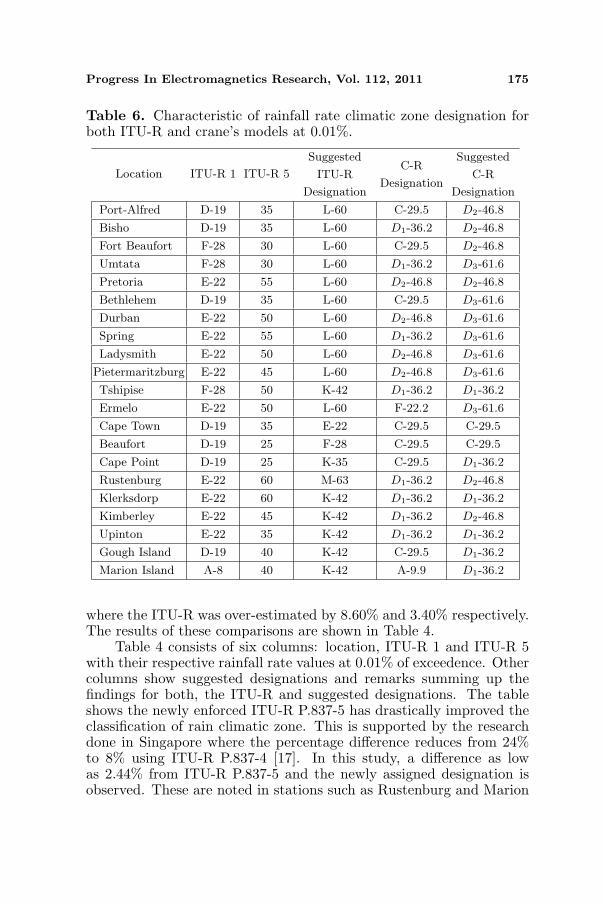
Table 6. Characteristic of rainfall rate climatic zone designation forboth ITU-R and crane’s models at 0.01%.

Location ITU-R 1 ITU-R 5

Suggested

ITU-R

Designation

C-R

Designation

Suggested

C-R

Designation

Port-Alfred D-19 35 L-60 C-29.5 D2-46.8

Bisho D-19 35 L-60 D1-36.2 D2-46.8

Fort Beaufort F-28 30 L-60 C-29.5 D2-46.8

Umtata F-28 30 L-60 D1-36.2 D3-61.6

Pretoria E-22 55 L-60 D2-46.8 D2-46.8

Bethlehem D-19 35 L-60 C-29.5 D3-61.6

Durban E-22 50 L-60 D2-46.8 D3-61.6

Spring E-22 55 L-60 D1-36.2 D3-61.6

Ladysmith E-22 50 L-60 D2-46.8 D3-61.6

Pietermaritzburg E-22 45 L-60 D2-46.8 D3-61.6

Tshipise F-28 50 K-42 D1-36.2 D1-36.2

Ermelo E-22 50 L-60 F-22.2 D3-61.6

Cape Town D-19 35 E-22 C-29.5 C-29.5

Beaufort D-19 25 F-28 C-29.5 C-29.5

Cape Point D-19 25 K-35 C-29.5 D1-36.2

Rustenburg E-22 60 M-63 D1-36.2 D2-46.8

Klerksdorp E-22 60 K-42 D1-36.2 D1-36.2

Kimberley E-22 45 K-42 D1-36.2 D2-46.8

Upinton E-22 35 K-42 D1-36.2 D1-36.2

Gough Island D-19 40 K-42 C-29.5 D1-36.2

Marion Island A-8 40 K-42 A-9.9 D1-36.2

where the ITU-R was over-estimated by 8.60% and 3.40% respectively.The results of these comparisons are shown in Table 4.

Table 4 consists of six columns: location, ITU-R 1 and ITU-R 5with their respective rainfall rate values at 0.01% of exceedence. Othercolumns show suggested designations and remarks summing up thefindings for both, the ITU-R and suggested designations. The tableshows the newly enforced ITU-R P.837-5 has drastically improved theclassification of rain climatic zone. This is supported by the researchdone in Singapore where the percentage difference reduces from 24%to 8% using ITU-R P.837-4 [17]. In this study, a difference as lowas 2.44% from ITU-R P.837-5 and the newly assigned designation isobserved. These are noted in stations such as Rustenburg and Marion

176 Owolawi

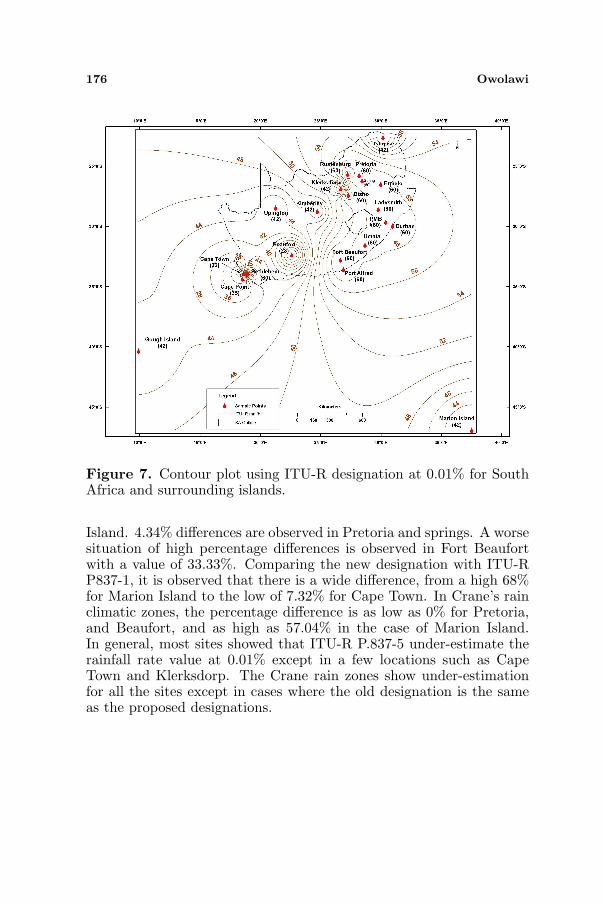
Figure 7. Contour plot using ITU-R designation at 0.01% for SouthAfrica and surrounding islands.

Island. 4.34% differences are observed in Pretoria and springs. A worsesituation of high percentage differences is observed in Fort Beaufortwith a value of 33.33%. Comparing the new designation with ITU-RP837-1, it is observed that there is a wide difference, from a high 68%for Marion Island to the low of 7.32% for Cape Town. In Crane’s rainclimatic zones, the percentage difference is as low as 0% for Pretoria,and Beaufort, and as high as 57.04% in the case of Marion Island.In general, most sites showed that ITU-R P.837-5 under-estimate therainfall rate value at 0.01% except in a few locations such as CapeTown and Klerksdorp. The Crane rain zones show under-estimationfor all the sites except in cases where the old designation is the sameas the proposed designations.

Progress In Electromagnetics Research, Vol. 112, 2011 177

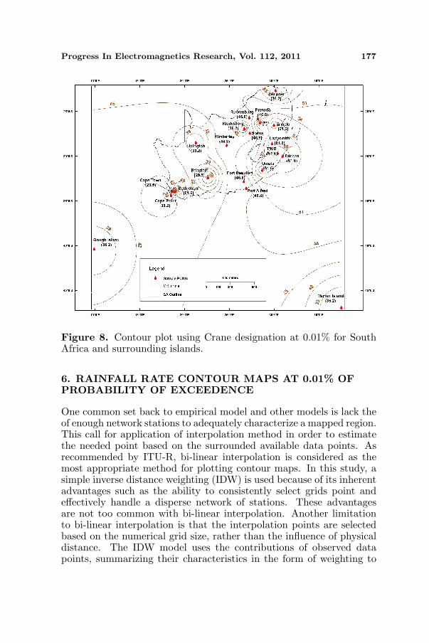
Figure 8. Contour plot using Crane designation at 0.01% for SouthAfrica and surrounding islands.

6. RAINFALL RATE CONTOUR MAPS AT 0.01% OFPROBABILITY OF EXCEEDENCE

One common set back to empirical model and other models is lack theof enough network stations to adequately characterize a mapped region.This call for application of interpolation method in order to estimatethe needed point based on the surrounded available data points. Asrecommended by ITU-R, bi-linear interpolation is considered as themost appropriate method for plotting contour maps. In this study, asimple inverse distance weighting (IDW) is used because of its inherentadvantages such as the ability to consistently select grids point andeffectively handle a disperse network of stations. These advantagesare not too common with bi-linear interpolation. Another limitationto bi-linear interpolation is that the interpolation points are selectedbased on the numerical grid size, rather than the influence of physicaldistance. The IDW model uses the contributions of observed datapoints, summarizing their characteristics in the form of weighting to

178 Owolawi

estimate the unknown points. The IDW expression is given by:

Zj = Kj

n∑

i=1

1dαij

Zi (17)

where Kj =n∑

i=1

1dij

is the adjustment that optimizes the weighting to

add up to 1 when the parameter α = 1. Using this estimator, we areable to provide for the unknown data points and draw contour mapsusing both ITU-R predicted rain rate (RR) and Crane designation at0.01% point for an easy application for radio planning engineers.

Figures 7 and 8 show the proposed rain climatic zones using a newproposed regional ITU-R and Crane model at 0.01% respectively. It isnoted from both figures that the eastern part of the map experiencesa higher rainfall rate distribution than the western part, with theexception of Bethlehem. This is as a result of the eastern wind fromthe Indian Ocean that hits the great escarpment that extends downto the tip of Bethlehem. Figures 7 and 8 confirmed the effect of theextensive wall, causing an orographic type of rainfall. In Figure 7,the tip of Cape Town, Upington and the islands recorded the lowestrainfall rate while the highest rainfall rate was recorded in the areassurrounded by the extensive coastal environment.

7. CONCLUSION

In this study, it is observed that the Western Cape region gets most ofits rainfall in winter, while the rest of the country is generally a summerrainfall region. The additional factors that contribute to this variationare the striking contrast between temperatures on the country’s eastand west coasts, and the contribution of the warm Agulhas and coldBenguela currents that sweep the coastlines. Being in the Southernhemisphere, the seasons stand in opposition to those of Europe andNorth America.

The most widely used probability distributions were investigatedusing the maximum likelihood estimator to optimize the distributions.It was found that most of the studied areas were best defined by theGamma distribution model, followed by Weibull distributions model,while Lognomal did well in very few sites. For the 21 stations, theGamma model had an average χ2 statistic of 10.8, followed by theWeibull model with an average of 19.85. The rest of the models gave anaverage χ2 statistic of above 55, which is too close to the threshold 63.7for 40 degree of freedom. The average root mean square percentagealso gives evidence to the fact that the Gamma model is the most

Progress In Electromagnetics Research, Vol. 112, 2011 179

appropriate to describe most sites in South Africa and its surroundingislands.

It is found in some sites that the ITU-R model that was usedover-estimates, while in many others sites the ITU-R model under-estimates, rainfall rate at defined points of probability of exceedences.Crane rain climatic zone designations had some exact matches in somesites as noted in Pretoria, Tshipise, Cape Town, Beaufort, Klerksdorpand Upington.

Rain contour maps have been identified as desirable tools forproviding system designers, site engineers and network planners withestimated fade margins due to rain attenuation. The two plottedcontour maps were optimized using statistical tool to satisfy acceptedrainfall climatic zones defined by the ITU-R and Crane maps whichare available in most radio planning tools. In this research, the contourmap was developed using advanced Geographic Information Systems(GIS) tools with the adoption of IDW estimator to provide the contourmap for rainfall rate at 0.01% of exceedence.

REFERENCES

1. Collin, R. E., Antennas and Radiowave Propagation, 401–402,McGraw Hill, ISBN 0-07-Y66156-1, 1995.

2. Goldhirsh, J., “Yearly variations of rain-rate statistics at wallopsisland and their impact on modeled slant path attenuationdistributions,” IEEE Transaction on Antennas and Propagation,Vol. 31, No. 6, 918–921, November 1983.

3. Crane, R. K., Electromagnetic Wave Propagation Through Rain,Wiley Interscience, New York, 1996.

4. ITU-R: Characteristics of Precipitation for Propagation Modeling,Recommendation P.837-4. ITU-R Recommendations, P Series,International Telecommunications Union, Geneva, 2007.

5. Rice, P. and N. Holmberg, “Cumulative time statistics of surface-point rainfall rate,” IEEE Transactions on Communications,Vol. 21, 1772–1774, October 1973.

6. Moupfounma, F. and L. Martin, “Modelling of the rainfallrate cumulative distribution for the design of satellite andterrestrial communication systems,” International Journal ofSatellite Communications, Vol. 13, No. 2, 105–115, 1995.

7. Ajayi, G. O. and E. B. C. Ofoche, “Some tropical rainfallrate characteristics at ile-ife for microwave and millimeter waveapplication,” Journal of Climate and Applied Meteorology, Vol. 23,562–567, 1983.

180 Owolawi

8. Owolawi, P. A., T. J. Afullo, and S. B. Malinga, “Effect of rainfallon millimeter wavelength radio in Gough and Marion Islands,”PIERS Online, Vol. 5, No. 4, 328–335, 2009.

9. Owolawi, P. A., T. J. Afullo, and S. B. Malinga, “Rainfall ratecharacteristics for the design of terrestrial links in South Africa,”Proceedings of Southern Africa Telecommunication Networks andApplications Conference (SATNAC), 1–76, September 2008.

10. Fashuyi, M. O., P. A. Owolawi, and T. J. Afullo, “Rainfall ratemodeling for LOS radio systems in South Africa,” South AfricanInstitute of Electrical Engineering Journal, Vol. 97, No. 1, 74–81,March 2006.

11. Owolawi, P. A. and T. J. Afullo, “Rainfall rate modeling and itsworst month statistics for millimetric LOS links in South Africa,”Radio Science, Vol. 42, 2007.

12. Owolawi, P. A., T. J. Afullo, and S. B. Malinga, “Effect ofworst-month distribution on radio link design in South Africa,”11th URSI Commission F Triennial Open Symposium on RadioWave Propagation and Remote Sensing, 55–61, Rio de Janeiro,October 2007.

13. Mulangu, C. T., P. A. Owolawi, and T. J. O. Afullo, “Rainfallrate distribution for LOS radio system in Botswana,” Proceedingsof 10th Southern Africa Telecommunication, Networks andApplication Conference (SATNAC), Mauritius, September 2007.

14. Owolawi, P. A., “Rain rate and rain drop size distributionmodels for line-of-sight millimetric systems in South Africa,”M.Sc. Dissertation, Department of Electrical and ElectronicsEngineering, University of KwaZulu Natal, Durban, 2006.

15. Seeber, R. J., “N model vir die bepaling van die punt-reenintensitverdeling vir die voorspelling van mikrogolf-reenverswakking in Suidelike Afrika,” South African Institute ofElectrical Engineering Journal, 67–75, June 1995.

16. Owolawi, P. A., “Characteristics of rain at microwave andmillimetric bands for terrestrial and satellite links attenuation insouth africa and surrounding islands,” Ph.D. Dissertation, Schoolof Electrical, Electronics and Computer Engineering, Universityof KwaZulu Natal, Durban, South Africa, 2010.

17. Emiliani, L. D., J. Agudelo, E. Gutierrez, J. Restrepo, andC. Fradique-Mendez, “Development of rain-attenuation and rain-rate maps for satellite system design in the Ku and Ka bands inColombia,” IEEE Antennas and Propagation Magazine, Vol. 46,No. 6, 54–68, December 2004.

18. World Meteorological Organization: World Distribution of

Progress In Electromagnetics Research, Vol. 112, 2011 181

Thunderstorm Days, No. 21, TP. 21, WMO/OMM, Geneva, 1953.19. World Meteorological Organization: World Meteorological Organi-

zation Climatological Normal (CLINO) for Climate and ClimateShip Stations for the Period 1931–1960, WMO/OMM, No. 117,TP. 52, Geneva, 1962.

20. Dutton, E. J., H. T. Dougherty, and R. F. Martin, Jr., “Predictionof European rainfall and link performance coefficients at 8 to30GHz,” NTIS Rep., ACC-ACO-16-17, 1974.

21. Wong, R. K. W., “Weibull distribution, iterative likelihoodtechniques and hydrometeorlogical data,” Journal of AppliedMeteorology, Vol. 16, 1360–1364, 1977.

22. Wilks, D. S., “Rainfall intensity, the Weibull distributionand estimation of daily surface runoff,” Journal of AppliedMeteorology, Vol. 28, 52–58, 1989.

23. Evans, M., N. Hastings, and B. Peacock, Statistical Distributions,2nd edition, John Wiley and Sons Inc., New York, 1993.

24. Walack, C., Hand-book on Statistical Distributions for Experimen-talists, Internal Report SUF-PFY/96-01, University of Stockholm,2007.

25. Eckhard, L., A. S. Werner, and A. Markus, “Lognormaldistributions across the sciences: Key and clues,” BioScience,Vol. 51, No. 5, May 2001.

26. Suhaila, J. and A. A. Jemain, “Fitting daily rainfall amount inMalaysia using the normal transformer distribution,” Journal ofApplied Science, Vol. 7, No. 14, 2007.

27. Thom, H. C., “A note on the gamma distribution,” MonthlyWeather Review, Vol. 86, 117–122, 1958.