Bayesian pattern recognition in optically-degraded noisy images

Rafael Navarro, Oscar Nestares, Jose J. Valles

Instituto de Óptica “Daza de Valdés”, Consejo Superior de Investigaciones Científicas

Serrano 121, 28006 Madrid, Spain.

Abstract

We present a novel Bayesian method for pattern recognition in images affected by

unknown optical degradations and additive noise. The method is based on a

multiscale/multiorientation subband decomposition of both the matched filter (original

object) and the degraded images. Using this image representation within the Bayesian

framework, it is possible to make a coarse estimation of the unknown Optical Transfer

Function, which strongly simplifies the Bayesian estimation of the original pattern that

most probably generated the observed image. The method has been implemented and

compared to other previous methods through a realistic simulation. The images are

degraded by different levels of both random (atmospheric turbulence) and deterministic

(defocus) optical aberrations, as well as additive white Gaussian noise. The Bayesian

method showed to be highly robust to both optical blur and noise, providing rates of

correct responses significantly better than previous methods.

Submitted to: Journal of Optics A: Pure and Applied Optics, May 13, 2011

PACS numbers: 42.30-d, 42.30.Va

2

1. Introduction

Pattern recognition is an extremely useful technique in image analysis, spanning a large variety

of applications1 from object recognition, to image retrieving and classification. Traditional

pattern recognition methods, based on matching or correlation, are highly attractive, but their

main drawback is that they are strongly sensitive to optical degradations and noise in the

observed images. There is a large number of references in the literature proposing correlation-

based pattern recognition methods to obtain invariant pattern recognition against different

transformations, distortions and all kinds of degradations of the image2. Many studies have

focused on geometric distortions, such as scaling and rotation3,4,5, and also on pattern recognition

or localization in the presence of noise 6, 7, 8, 9, 10. Less work has been done in optically degraded

images11, where most of the published works deal with the particular case of defocus12,13. There

is however a lack of methods able to deal robustly with images doubly degraded by the

combined effect of optical aberrations (or scattering) and noise.

In this work, we propose and test a novel Bayesian approach, for pattern recognition robust to the

combined effect of optical degradations (aberrations, etc.) and noise on the image. The Bayesian

approach consists of a probabilistic formulation, classic in many estimation or decision-making

problems, which has also been used in pattern recognition9. In a previous publication, Vargas et

al.13 obtained invariant pattern recognition against defocus by first applying a subband

decomposition of the matched filter, and then combining the correlation outputs of each channel

in a multiplicative way. This showed to be a highly efficient method to remove potential false

alarms, which otherwise would soon appear with defocus. Based on that work, we have

generalized the method, by introducing a probabilistic Bayesian framework that permits us to

deal with a more general form for the optical degradation (modelled as an Optical Transfer

3

Function linear filter) and to include additive noise. Here, we make use of a subband

decomposition, but instead of the multiscale Laplacian pyramid14 used in Ref. 13 to deal with

pure defocus, here we apply a multiscale/multiorientation Gabor pyramid15, which permits us to

deal with more general non-symmetric optical degradations.

There are situations where optical degradations are constant or can be calibrated somehow, so

that this a priori knowledge can be available to the recognition algorithm. However, in the

present study, we are interested in the cases where the optical degradation is unknown, such as

image degradations introduced by random or unpredictable motion, atmospheric turbulence, or

turbid media in general. The proposed Bayesian method implicitly estimates a coarse

approximation of the Optical Transfer Function (OTF) to find the pattern that most probably

generated the observed image.

To test the different methods, including the one proposed here, we have carried out a realistic

simulation where the task was to classify flying birds (different eagles and falcons species)

observed through a telescope in the presence of atmospheric turbulence. The images were also

affected by additive Gaussian noise. Our method, which compares favourably with other

previous approaches, provided high recognition rates even for large optical degradations and low

signal to noise ratios.

4

2. Methods

The Bayesian method consists of three main elements: (1) An observation model consisting of

linear filtering of the object with the OTF and additive noise; (2) a multiscale/multiorientation

decomposition of the image giving rise to a set of observed subbands; and (3) a Bayesian

framework to estimate the pattern that most probably generated the observed image, as well as a

coarsely sampled estimate of the OTF.

The optical degradation is modelled as a generic complex low-pass linear filter. Its modulus, the

modulation transfer function (MTF), causes contrast attenuation to the different spatial

frequencies in the object, while the Phase Transfer Function (PTF) produces a different shift to

each spatial frequency. The proposed method explicitly assumes that the OTF is unknown, and

the strategy is to implicitly estimate the OTF during the recognition process. The blur in the

image domain is given by the Point Spread Function (PSF) that is the Fourier transform of the

OTF.

Therefore, we have to consider that, for an optimal recognition performance, we have to

simultaneously estimate two unknowns, the original pattern and the OTF. The main problem

with this general approach is that is not well-to constrained, and therefore to solve this double

estimation (or recognition) problem we need include some a priori information, which is

straightforward in the Bayesian framework.

Using a priori knowledge, we can make approximations that permit us to constrain the

recognition problem. First we apply a most usual constraint, based on the assumption that the

object belongs to a finite set of possible objects. For instance in character recognition, the object

5

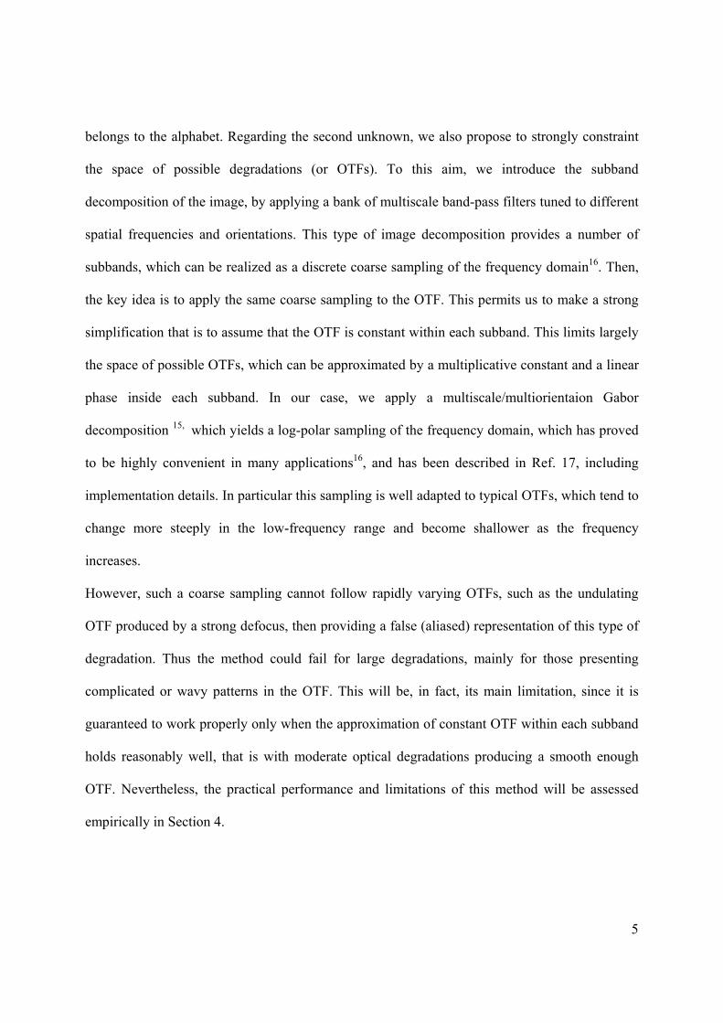
belongs to the alphabet. Regarding the second unknown, we also propose to strongly constraint

the space of possible degradations (or OTFs). To this aim, we introduce the subband

decomposition of the image, by applying a bank of multiscale band-pass filters tuned to different

spatial frequencies and orientations. This type of image decomposition provides a number of

subbands, which can be realized as a discrete coarse sampling of the frequency domain16. Then,

the key idea is to apply the same coarse sampling to the OTF. This permits us to make a strong

simplification that is to assume that the OTF is constant within each subband. This limits largely

the space of possible OTFs, which can be approximated by a multiplicative constant and a linear

phase inside each subband. In our case, we apply a multiscale/multiorientaion Gabor

decomposition 15, which yields a log-polar sampling of the frequency domain, which has proved

to be highly convenient in many applications16, and has been described in Ref. 17, including

implementation details. In particular this sampling is well adapted to typical OTFs, which tend to

change more steeply in the low-frequency range and become shallower as the frequency

increases.

However, such a coarse sampling cannot follow rapidly varying OTFs, such as the undulating

OTF produced by a strong defocus, then providing a false (aliased) representation of this type of

degradation. Thus the method could fail for large degradations, mainly for those presenting

complicated or wavy patterns in the OTF. This will be, in fact, its main limitation, since it is

guaranteed to work properly only when the approximation of constant OTF within each subband

holds reasonably well, that is with moderate optical degradations producing a smooth enough

OTF. Nevertheless, the practical performance and limitations of this method will be assessed

empirically in Section 4.

6

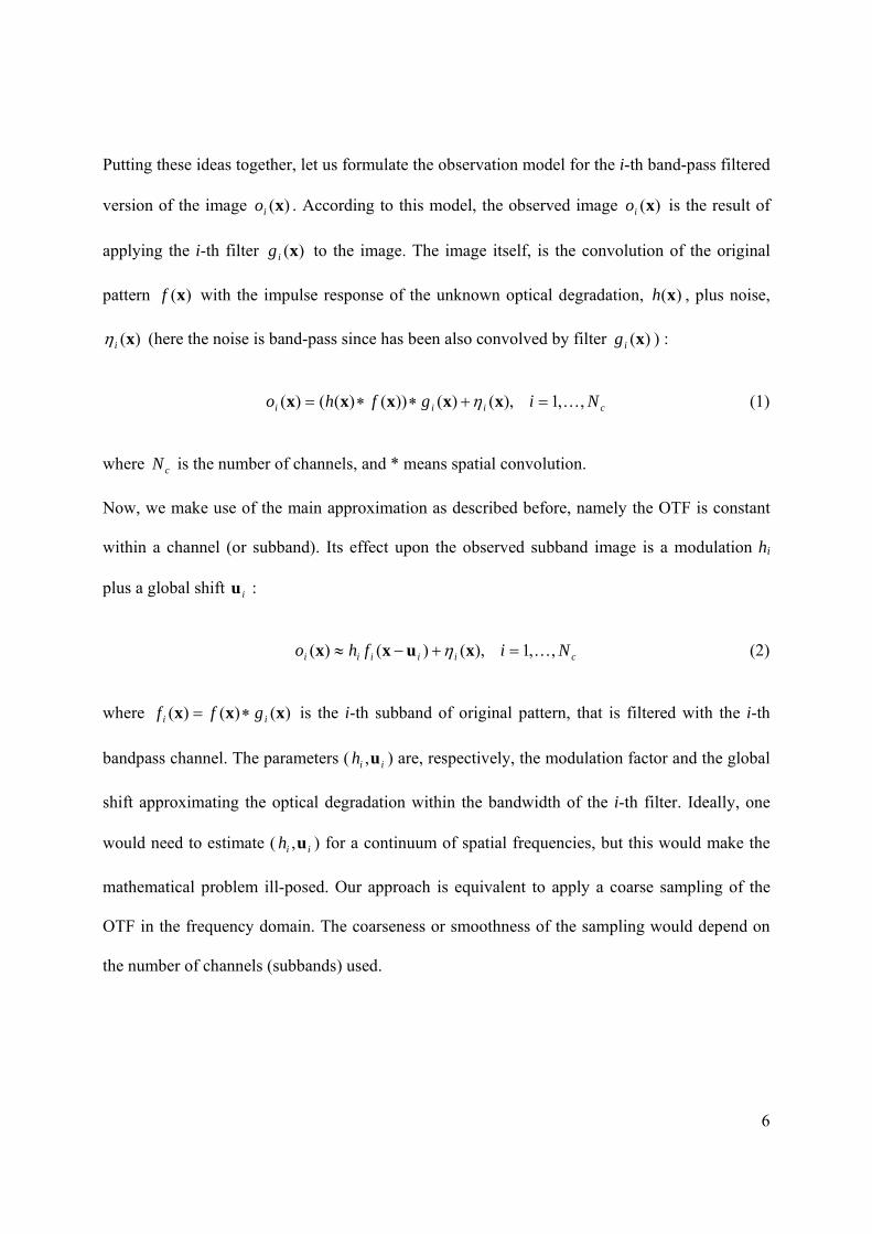
Putting these ideas together, let us formulate the observation model for the i-th band-pass filtered

version of the image )(xio . According to this model, the observed image )(xio is the result of

applying the i-th filter )(xig to the image. The image itself, is the convolution of the original

pattern )(xf with the impulse response of the unknown optical degradation, )(xh , plus noise,

)(xi (here the noise is band-pass since has been also convolved by filter )(xig ) :

ciii Nigfho ,,1),()())()(()( xxxxx (1)

where cN is the number of channels, and * means spatial convolution.

Now, we make use of the main approximation as described before, namely the OTF is constant

within a channel (or subband). Its effect upon the observed subband image is a modulation hi

plus a global shift iu :

ciiiii Nifho ,,1),()()( xuxx (2)

where )()()( xxx ii gff is the i-th subband of original pattern, that is filtered with the i-th

bandpass channel. The parameters ( iih u, ) are, respectively, the modulation factor and the global

shift approximating the optical degradation within the bandwidth of the i-th filter. Ideally, one

would need to estimate ( iih u, ) for a continuum of spatial frequencies, but this would make the

mathematical problem ill-posed. Our approach is equivalent to apply a coarse sampling of the

OTF in the frequency domain. The coarseness or smoothness of the sampling would depend on

the number of channels (subbands) used.

7

Given this strongly simplified observation model, we can now formulate the joint posterior

probability for the original input pattern f, and for the approximated linear degradation model

parameters },{ iih u . Given the observations }{ io and applying Bayes rule we obtain:

}),({)(}),{,|}({}){|},{,( iiiiiiii hpphpKhp ufufoouf (3)

where for notational convenience, we have expressed images as intensity vectors; K is a

normalization constant. The posterior probability is proportional to the likelihood (or conditional

probability of the observations, given the input pattern and the degradation parameters)

multiplied by the prior probability. In the previous expression we have assumed that the input

pattern f is statistically independent of the linear degradation model parameters },{ iih u . If we

further assume a constant prior probability for the degradation parameters },{ iih u , then the

posterior probability is finally:

)(}),{,|}({}){|},{,( fufoouf phpKhp iiiiii (4)

where K’ is another normalization constant. The Maximum A Posteriori (MAP) estimator for the

input pattern f and for the linear degradation parameters }ˆ,ˆ{ iih u is the one that maximizes the

posterior probability in Eq. 4:

)(}),{,|}({maxarg})ˆ,ˆ{,ˆ(}),{,(

fufoufuf

phph iiih

iiii

(5)

where the likelihood function }),{,|}({ iii hp ufo is given by the probability density function of

the noise i

p , according to the observation model in Eq. 2. If we further assume conditional

8

independence between channels and between spatial locations inside the channels, the likelihood

is then given by

c

i

N

iiiiiiii fhophp

1

)()(}),{,|}({x

uxxufo . (6)

Now, we can incorporate all the a priori information as a prior probability on the input image f .

From the assumptions of the recognition problem, we know that the input image belongs to a

finite set Nj

j1}{ f , where N is the total number of patterns. The assumption of having a limited set

of possible patterns heavily constrains the space of all the possible intensity configurations of the

input image, resulting in a posterior probability that is different from 0 only when Nj

j1}{ ff :

c

i

N

ii

jiiiiii

j fhophp1

)()(}){|},{,(x

uxxouff . (7)

Here we have assumed that all the patterns jf are equiprobable a priori, but in case that they

were not equiprobable, it would be straightforward to include the appropriate probabilities as

simple weights in Eq. 7. Therefore, the recognition of an input pattern consists of first choosing

the degradation parameters maximizing the probability in Eq. 7 for every pattern in the alphabet,

and then choosing the pattern with the largest probability, which will give us the global

maximum of the posterior probability distribution. Such maximization can be done separately for

each channel, and then multiplying the maximum probability values afterwards. For channel i,

and assuming white Gaussian noise, the maximization of the probability is equivalent to the

minimization of the following error function:

x

uxx2

)()( ij

iiij

i fhoE . (8)

9

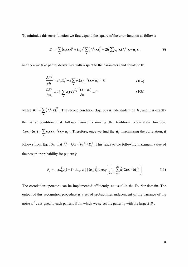
To minimize this error function we first expand the square of the error function as follows:

xxx

uxxxx )()(2)()()(222

ij

iiij

iiij

i fohfhoE , (9)

and then we take partial derivatives with respect to the parameters and equate to 0:

where x

x2

)(ji

ji fK . The second condition (Eq.10b) is independent on ih , and it is exactly

the same condition that follows from maximizing the traditional correlation function,

x

uxxu )()()( ij

iiij

i foCorr . Therefore, once we find the jiu maximizing the correlation, it

follows from Eq. 10a, that ji

ji

ji

ji KCorrh /)ˆ(ˆ u . This leads to the following maximum value of

the posterior probability for pattern j:

cN

i

ji

ji

jiiii

jj CorrhhpP

12

)ˆ(ˆ2

1exp}){|},{,(max uouff

(11)

The correlation operators can be implemented efficiently, as usual in the Fourier domain. The

output of this recognition procedure is a set of probabilities independent of the variance of the

noise 2 , assigned to each pattern, from which we select the pattern j with the largest jP .

x

x

u

uxx

u

uxx

0)(

)(2

0)()(22

i

ij

iii

i

ji

ij

iij

iii

ji

foh

E

foKhh

E(10a)

(10b)

10

3. Implementation and numerical experiments

To test the model, we have conducted a realistic computer simulation, in which the scenario

consists of the problem of identification of different species of eagles and falcons, viewed

through atmospheric turbulence, with added defocus and noise. The outputs of these simulations

are the input blurred images used to test the proposed method, as shown in Figure 1. Other

previous methods have been also implemented for comparison purposes, as explained next.

3.1. Pattern recognition methods

3.1.1. Bayesian

To implement the Bayesian method, one has to choose the subband decomposition. We have

used an efficient implementation¡Error! Marcador no definido. of a Gabor multiscale/multioriorientation

pyramid. The parameters of the Gabor filter bank have been chosen to provide a good sampling

of the Fourier domain while maintaining computational efficiency, and are the following:

Bandwidth (measured along the radial direction) of 1 octave.

Form factor of 1 (isotropic Gaussian envelope).

4 scales distributed in octaves.

Highest radial tuning frequency of 1/4 cycles/sample.

4 principal orientations (0, 45, 90 and 135 deg).

With these parameters it is possible to implement the filter bank very efficiently in the spatial

domain, using separable convolutions and a pyramidal strategy to obtain the coarser scales.

11

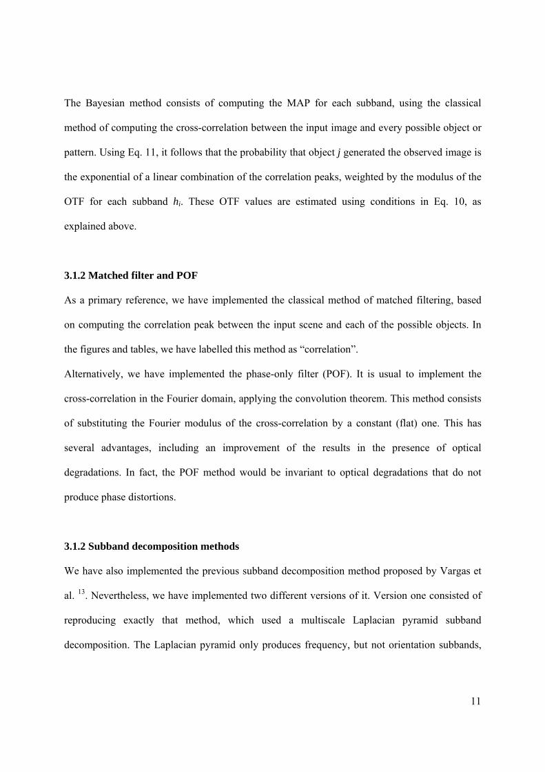
The Bayesian method consists of computing the MAP for each subband, using the classical

method of computing the cross-correlation between the input image and every possible object or

pattern. Using Eq. 11, it follows that the probability that object j generated the observed image is

the exponential of a linear combination of the correlation peaks, weighted by the modulus of the

OTF for each subband hi. These OTF values are estimated using conditions in Eq. 10, as

explained above.

3.1.2 Matched filter and POF

As a primary reference, we have implemented the classical method of matched filtering, based

on computing the correlation peak between the input scene and each of the possible objects. In

the figures and tables, we have labelled this method as “correlation”.

Alternatively, we have implemented the phase-only filter (POF). It is usual to implement the

cross-correlation in the Fourier domain, applying the convolution theorem. This method consists

of substituting the Fourier modulus of the cross-correlation by a constant (flat) one. This has

several advantages, including an improvement of the results in the presence of optical

degradations. In fact, the POF method would be invariant to optical degradations that do not

produce phase distortions.

3.1.2 Subband decomposition methods

We have also implemented the previous subband decomposition method proposed by Vargas et

al. 13. Nevertheless, we have implemented two different versions of it. Version one consisted of

reproducing exactly that method, which used a multiscale Laplacian pyramid subband

decomposition. The Laplacian pyramid only produces frequency, but not orientation subbands,

12

so that it is multiscale, but not multiorientation. We have labelled this version of the method as

“Laplacian”. For a more direct comparison with our Bayesian approach, we have also

implemented a second version of the subband decomposition method, simply changing the

Laplacian by the same Gabor pyramid used in the Bayesian method. We use the label Gabor for

the resulting method. These two different versions could show a rather different performance,

because in the subband method, the combination of subbands consists of computing the product

of correlation13, so that if we have a significantly higher number of subbands, such as in the

Gabor case, this could strongly affect the performance.

Therefore, we have implemented five different methods: Bayesian, correlation, POF, Laplacian

and Gabor.

3.2 Simulation of atmospheric turbulence

A realistic simulation has been implemented, where the objects are different types of flying

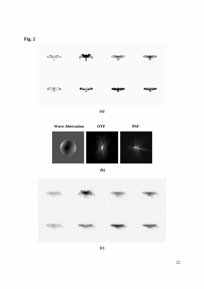
eagles and falcons (see Fig. 2a). The birds are highly similar in size and overall shape, but

exhibit differences mainly in the patterns formed by the feathers, tail or wings shape, and other

details. Thus, the discrimination and identification of each species is not straightforward even in

optimal viewing conditions. These objects are viewed through a telescope from the ground in the

presence of random aberrations induced by atmospheric turbulence. We have considered short-

exposure or instantaneous images, in the sense that each image corresponds to a single

realization of the random fluctuations. Here, the Zernike coefficients describing the atmospheric

optical aberrations are computed based on the classic the Kolmogorov model18. In particular, the

data used here were kindly provided by Cagigal and Canales from the University of Cantabria

(Spain), who used their own simulation tool19. The statistics of the aberrations is determined by

13

the parameter D/r0 , where D is the pupil diameter of the telescope and r0 is the Fried parameter,

or atmospheric correlation length. As a simplification, we have considered monochromatic light,

with wavelength 550 nm. The scale of the different species has been equalized so that the

wingspan is about one meter, and we have considered two viewing distances, of about 90 m., and

180 m. These viewing distances produce images with different scales. In the figures, we refer to

100% scale to the case of 90 m. viewing distance, and 50% to the 180 m. case, respectively. The

scale of the point spread function, has been adjusted to match these sizes, considering D = 20 cm.

In addition to turbulence, different defocus and additive noise conditions have been simulated, as

shown in Table 1. Each image is simulated by first computing the OTF from the Zernike

coefficients (wave aberration) of the atmospheric turbulence, plus and added amount of defocus.

The input object, is introduced as a 128x128 pixels image (see Fig. 2), and is filtered by the

simulated OTF, and finally three different levels of random Gaussian noise are added to the

filtered image.

The complete set of conditions is summarized in Table 1. Thus, the total number of images

generated in the simulation is 8 (birds) x 10 (random realizations) x 3 (D/r0) x 6 (defocus level) x

3 (SNR) x 2 (distance) = 8640. This large number of images permits us to make some statistics

on the behaviour of the five different methods. Fig. 2(c) shows a typical realization of observed

images where the degradation suffered by the original images is manifest, so that the recognition

is not so easy even for a human observer. The conditions of this particular example are: D/r0 = 2,

defocus = λ/2, SNR = 1, full 100% size (90 m viewing distance).

14

4. Results

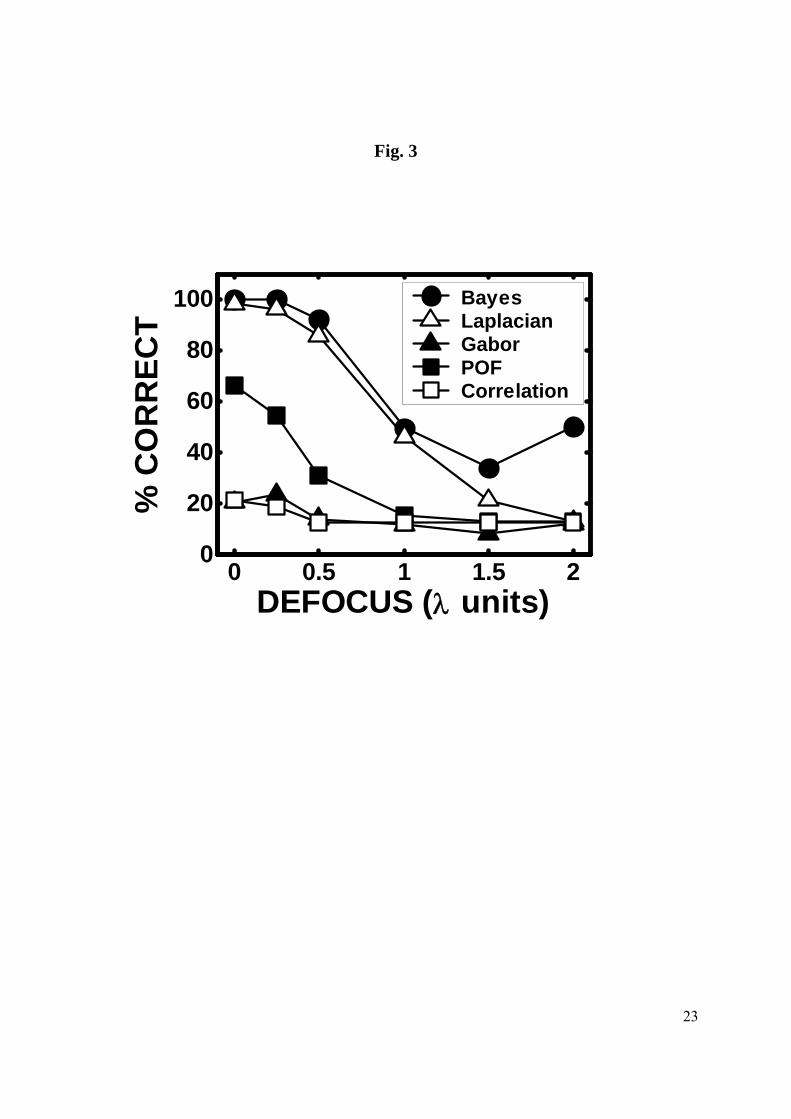
Figure 3 compares the global averages of the percentage of correct responses provided by the

different methods as a function of defocus. In this case, only the highest SNR = 20 has been

considered. If we take into account that for defocus = 0 only the atmospheric turbulence is

degrading the image, it is clear that only the Bayesian and the Laplacian pyramid methods show

a high tolerance to this type of degradation. The correlation and Gabor methods provide poor

results just above chance levels (chance level =12.5%), whereas the phase-only filter provides

about 60 % correct responses. This percentage of the POF method mainly reflects an unequal

behaviour: a high rate of correct answers for the easier conditions (low turbulence, and 100%

scale) and a poor rate for the more difficult ones (high turbulence and 50% scale), where the POF

performance drops rapidly. Regarding the evolution of the curves with defocus, there is a small

but important difference between the two best methods. The Bayesian method ensures the 100 %

correct responses, even in the presence of small amount of defocus (/4). The Laplacian method

goes basically parallel, just below the Bayesian one, but reaches the chance level for the

maximum defocus (2. On the contrary, the Bayesian method does not decay to chance level

even for that high defocus.

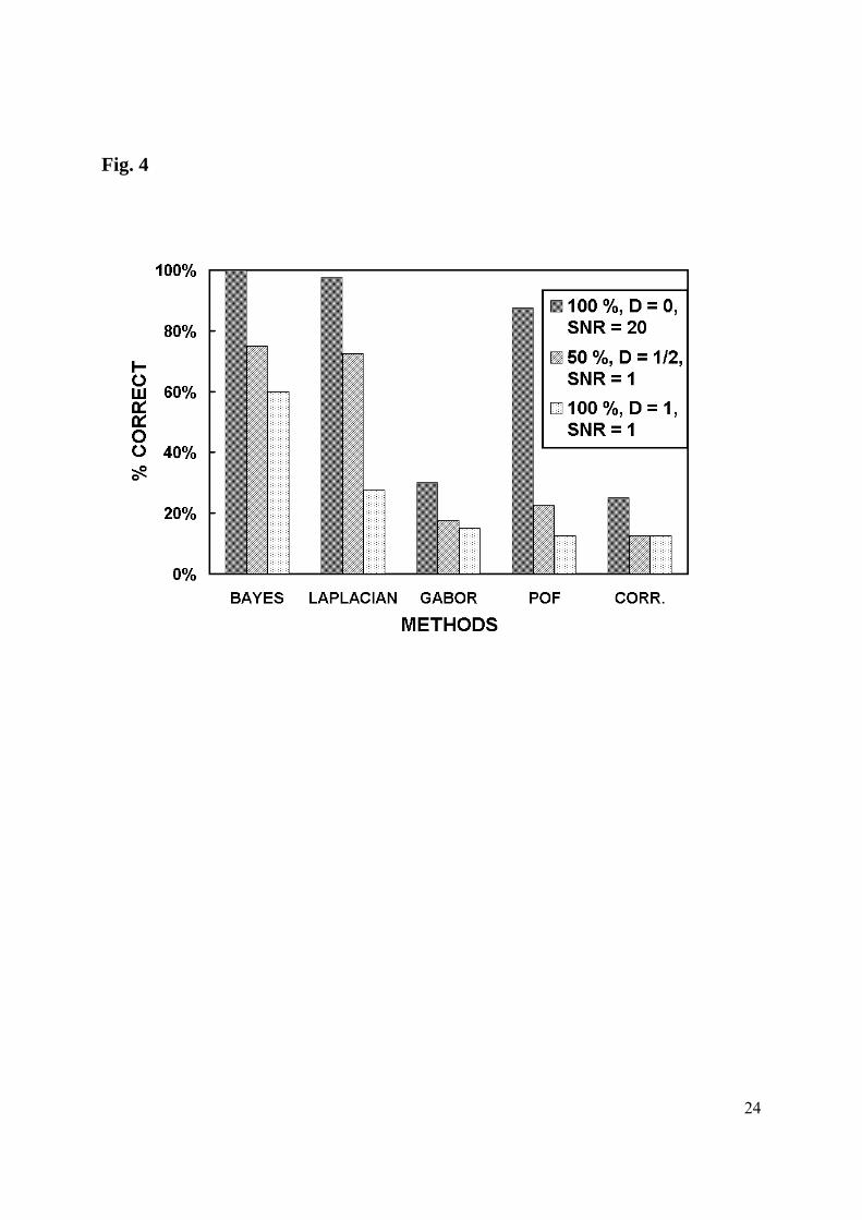
Figure 4 compares the percent of correct responses for three of the conditions tested. The first

case corresponds to the best or easiest condition (scale = 100%, defocus = 0, SNR = 20); the

second is a difficult condition, with far distance and a very low SNR, but a moderate-low

defocus (scale= 50%; defocus = , SNR = 1); the third condition corresponds to a more serious

defocus, with full scale of the object and the same very low SNR (scale= 100%; defocus = ,

SNR = 1). The Bayesian method always provides percent correct responses above 60% (and

15

equals 100% for 0 defocus). The Laplacian method shows a high performance for small amounts

of defocus, just below the Bayesian one, but drops for important defocus amounts. The phase-

only filter does a good job when there is no defocus and the SNR is high, but it hardly tolerates

the combined effect of defocus and noise. Again the Gabor and correlation methods perform

poorly.

The global percent correct responses for the complete set of conditions and realizations are listed

in Table 2 for each method. The Bayesian method performs clearly higher than the other

methods. That was true for all conditions tested except for scale = 50%, and defocus = λ, where

the product of correlations of Laplacian channels was slightly superior. The average result

obtained with the proposed Bayesian method confirms that (71% of correct responses, in contrast

to the 60% correct provided by the product of Laplacian correlations). Apart from these two

methods, both the product of Gabor correlations, and the standard correlation methods only

reached 15% of correct responses that is a rather poor performance just above chance level

(12.5%). Only the phase-only filter performed clearly above chance level providing a 33%

correct answers, but far from the two first methods.

16

5. Conclusions

We have presented a novel Bayesian method for pattern recognition in images degraded by

unknown general optical degradations and additive noise. The results presented here show that

the proposed method is highly robust against these optical degradation and noise in the observed

image. Our results are consistent with previous works in the sense that the standard correlation,

or matched filter method hardly support optical degradations. The phase-only filter method is

much more robust against optical degradations, but it fails when the optical aberrations induce

phase distortions in the OTF. The method by Vargas et al. 13, based on the product of correlations

of the Laplacian pyramid decomposition, performs much better than those previous methods, but

worse than the proposed Bayesian method, especially for large degradations. The Bayesian

method is able to produce reasonable results for the broad class of conditions tested. The coarse

approximation introduced for the optical degradation can be interpreted as a regularization that

gives a well-conditioned problem from the ill-conditioned problem that would try to estimate the

full OTF of the degradation from the observed image. The method will fail if the OTF changes

rapidly or abruptly. In this case, we would need to increase the number of channels to sample

more finely the Fourier domain, but there is a trade-off between sampling finely the Fourier

domain and regularizing the ill-posed problem. The main advantage is its generic degradation

model, which is not restricted to defocus, and that includes naturally the noise in the Bayesian

framework. Finally, because the method is Bayesian it can be easily adapted to introduce priors

on the parameters of the coarse approximation of the degradation’s OTF, as well as on the

relative abundance of each pattern. Moreover, we can also introduce different costs or penalties

when the method fails to recognize the different patterns, which provides a great flexibility for

specific applications.

17

Acknowledgements

This research was partly supported by the Comisón Interministerial de Ciencia y Tecnología

under grant DPI2002-04370-C02-02. We want to thank Manuel P. Cagigal and Vidal F. Canales

who kindly provided us atmospheric turbulence aberration data.

REFERENCES

1 B. Javidi ed., "Image Recognition and Classification: Algorithms, Systems, and Applications," Marcel-Dekker, New York (2002). 2 F. Chan, N. Towghi, L. Pan, and B. Javidi, "Distortion Tolerant Minimum Mean Squared Error Filter for Detecting Noisy Targets in Environmental Degradations", J. Opt. Eng., 39, 2092-2100, (2000). 3 D. Casasent and D. Psaltis, “Scale Invariant Optical Correlation Using Mellin Transforms,” Optics Communications, 17, 59-63 (1976). 4 Y. N. Hsu and H. H. Arsenault, “Optical pattern recognition using circular harmonic expansion,” Applied Optics, 21, 4016–4019 (1982). 5 O. Gualdron and H. H. Arsenault, “Improved invariant pattern recognition methods,” in Real Time Optical Information Processing. B. Javidi and J. Horner, eds., Academic San Diego, Calif., 1994, pp. 89–113. 6 A. Fazlolahi and B. Javidi, "Error Probability of an Optimum Receiver Designed for Pattern Recognition with Nonoverlapping Target and Scene Noise", J. Opt. Soc. Am. A, 14, 1024-1032 (1997). 7 N. Towghi, B. Javidi and J. Li, " Generalized Optimum Receiver for Pattern Recognition with Multiplicative, Additive, and Nonoverlapping Noise", J. Opt. Soc. Am. A, 15, 1557-1565 (1998). 8 B.V.K. Vijaya Kumar, “Tutorial Survey of Correlation Filters for Optical Pattern Recognition,” Applied Optics, 31, 4773-4801 (1992)

18

9 P. Refregier, “Bayesian theory for target location in noise with unknown spectral density”, J. Opt. Soc. Am. A, 16, 2, 276-283 (1999). 10 N. Towghi and B. Javidi, "Optimum Receivers for Pattern Recognition in the Presence of Gaussian Noise with Unknown Statistics," J. Opt. Soc. Am. A, 18, 1844-1852, (2001). 11 S. Bosch, J. Campos, M. Montes-Usategui and J. Sallent , “Design of correlation filters invariant to degradations characterizable by an optical transfer function,” Optics Communications, 129, 5-6, 337-343 (1996). 12 A. Carnicer, S. Vallmitjana, J.R. de F. Moneo and I. Juvells, “Implementation of an algorithm for detecting patterns in defocused scenes using binary joint transform correlation,” Optics Communications, 130, 4-6, 327-336 (1996). 13 A. Vargas, J. Campos and R. Navarro, “Invariant pattern recognition against defocus based on subband decomposition of the filter,” Optics Communications, 185, 1-3, 33-40 (2000). 14 O.J. Burt, and F. H. Adelson, “The Laplacian pyramid as a compact image code”, IEEE Trans on Comm., 31, 532-540 (1983). 15 R. Navarro and A. Tabernero, “Gaussian wavelet transform: two alternative fast implementations for images,” Multidimensional Sys. Sig. Proc., 2, 421–436 (1991). 16 R. Navarro, A. Tabernero and G. Cristobal, “Image Representation with Gabor Wavelets and Its Applications,” in Advances in Imaging and Electron Physics, P. W. Hawkes editor, Academic Press, San Diego, 1996 (pp 1-84). 17 O. Nestares, R. Navarro, J. Portilla, and A. Tabernero, ‘‘Efficient spatial-domain implementation of a multiscale image representation based on Gabor functions,’’ J. Electron. Imaging 7,166–173 (1998). 18 R. J. Noll, “Zernike polynomials and atmosferic turbulence”, J. Opt. Soc. Am., 66, 207-211 (1976). 19 M. P. Cagigal y V. F. Canales, “Generalized Fried parameter after adaptive optics partial wave-front compensation”, J. Opt. Soc. Am. A, 17, 903-910 (2000).

Table. 1. Summary of all the conditions considered in the simulations

Objects (eagles and falcons) 8

Number of random realizations of turbulence per condition

10

D/r0 1 2 4

Defocus ( units) 0 λ/4 λ/2 λ 3λ/2 2λ

SNR 20 10 1

Viewing distance 90 m 180 m

Table. 2. Global average of the results obtained for each of the different methods tested

Methods Bayesian Laplacian Gabor POF Correlation

Global percent correct 71 60 15 33 15

20

FIGURE CAPTIONS

Fig. 1.- Schematic block diagram of the Bayesian pattern recognition method. A filter bank is

applied to both the set of patterns and to the input degraded image. Then the Bayesian method

gives the probabilities that the input image corresponds to the different pattern. The output

response is the pattern with maximum probability.

Fig. 2.- Realistic computer simulation: (a) The set of patterns considered. They correspond to

different eagle species. (b) One realization of the optical degradation. The Wave Aberration (left)

has random (turbulence) and deterministic (defocus) parts. The corresponding OTF and PSF are

also shown. (c) Degraded images obtained by filtering each pattern with the OTF and adding

random noise.

Fig. 3.- Percentage of correct responses as a function of defocus for the five methods compared:

Bayesian (black circles) , Laplacian (open triangles), Gabor (black triangles), POF (black

squares) and standard correlation (open squares).

Fig. 4.- Comparison of the performance of the methods for three particular conditions:

scale=100%, Defocus=0 and SNR=20 (dark); scale=50%, Defocus=/2 and SNR=1 (grey);

scale= 100%, Defocus= and SNR=1 (light grey).

21

Fig. 1.-

Set ofprobabilities

Maximumselection

Filter bank

Bayesianrecognition

Observed degraded image

Recognized pattern

Set of original images

Filter bank

Set ofprobabilities

Maximumselection

Filter bank

Bayesianrecognition

Observed degraded imageObserved degraded image

Recognized pattern

Set of original imagesSet of original images

Filter bank

22

Fig. 2

(a)

Wave Aberration OTF PSF

(b)

(c)

23

Fig. 3

0 0.5 1 1.5 20

20

40

60

80

100

DEFOCUS ( units)

% C

OR

RE

CT

BayesLaplacianGaborPOFCorrelation

24

Fig. 4