Radiating Flows - FAS
43
8 Radiating Flows In a radiating fluid, radiation affects the energy and momentum balance in the flow, and can drive the thermodynamic state of the material out of equilibrium. In this chapter we consider a few interesting examples of radiating-flow problems in both the linear and nonlinear regimes. For small-amplitude disturbances we focus on radiative energy and momentum exchange; we first examine the radiative smoothing of temper- ature fluctuations in a static medium, then the eflects of radiation on acoustic waves in a homogeneous medium, and finally the effects of radiation on acoustic-gravity waves in a stratified medium. We shall draw our examples primarily from astrophysics where considerable attention has been given to radiative effects on the propagation and dissipation of waves in the atmospheres of the Sun and stars. For nonlinear disturbances we meet a much richer variety of phenomena. We consider first the conceptually simple problem of penetra- tion of radiation into a passive static medium as a thermal wave. We then examine the effects of radiMiVe transport across steady shocks and in propagating shocks in both the weak- and strong-shock limits, including the case of a propagating non-LTE shock, where radiation determines the state of the material. We next examine the interplay of radiation and hydrodynamics in propagating ionization fronts. Finally, we consider the dynamics of radiation-driven stellar winds, where the primary effect of radiation is on the momentum balance in the flow. The reader should note that in most of the applications to be discussed the treatment of radiation falls far below the standards set in Chapter 7, although reasonably complete and consistent solutions are obtained for one or two simple problems. We make this remark not as a criticism of the existing literature, but rather to call attention to the rewarding oppor- tunities that exist for new research exploiting the more complete formula- tion of the dynamical behavior of radiation that is now available. 8.1 Small-Amplitude Disturbances 100. Radiative Damping of ‘Temperature Fluctuations Valuable insight into the effects of radiative energy exchange on small- amplitude disturbances can be obtained by examining the smoothing of temperature fluctuations in a radiating fluid. 507
Transcript of Radiating Flows - FAS

8
Radiating Flows
In a radiating fluid, radiation affects the energy and momentum balance inthe flow, and can drive the thermodynamic state of the material out ofequilibrium. In this chapter we consider a few interesting examples ofradiating-flow problems in both the linear and nonlinear regimes.
For small-amplitude disturbances we focus on radiative energy andmomentum exchange; we first examine the radiative smoothing of temper-ature fluctuations in a static medium, then the eflects of radiation onacoustic waves in a homogeneous medium, and finally the effects ofradiation on acoustic-gravity waves in a stratified medium. We shall drawour examples primarily from astrophysics where considerable attention hasbeen given to radiative effects on the propagation and dissipation of wavesin the atmospheres of the Sun and stars.
For nonlinear disturbances we meet a much richer variety ofphenomena. We consider first the conceptually simple problem of penetra-tion of radiation into a passive static medium as a thermal wave. We thenexamine the effects of radiMiVe transport across steady shocks and in
propagating shocks in both the weak- and strong-shock limits, includingthe case of a propagating non-LTE shock, where radiation determines thestate of the material. We next examine the interplay of radiation andhydrodynamics in propagating ionization fronts. Finally, we consider thedynamics of radiation-driven stellar winds, where the primary effect ofradiation is on the momentum balance in the flow.
The reader should note that in most of the applications to be discussedthe treatment of radiation falls far below the standards set in Chapter 7,although reasonably complete and consistent solutions are obtained for oneor two simple problems. We make this remark not as a criticism of theexisting literature, but rather to call attention to the rewarding oppor-tunities that exist for new research exploiting the more complete formula-tion of the dynamical behavior of radiation that is now available.
8.1 Small-Amplitude Disturbances
100. Radiative Damping of ‘Temperature Fluctuations
Valuable insight into the effects of radiative energy exchange on small-amplitude disturbances can be obtained by examining the smoothing oftemperature fluctuations in a radiating fluid.
507
508 FOUNDATIONS OF RADIATION HYDRODYNAMICS
QUASJ-SIATIC RADIATION ‘WUWSPOR~
Consider a field of temperature perturbations imposed on a static, grey,LTE ambient medium, initially in radiative equilibrium. We assume thereare no fluid motions (v= O), and that heat is exchanged only radiatively.Under these assumptions the gas energy equation (96.7) reduces to
p(de/dt) = 47TK(~-~), (100.1)
where, from (52.21 ), (de/dt) = c. (dT/i)t)in a static medium. The thermal
source is B = (a~c/47r) Td, and the mean intensity is 4rr.1 = $1 dco. Weassume that the characteristic time scale associated with the disturbances isso long that the radiation field can be taken to be quasi-static. Then 1 isgiven by the static transfer equation
(dr/ds) = K(B -1)> (100.2)
where s is the path length along a ray. In using (100.2) we neglect alldynamical effects of the radiation field.
For small disturbances we linearize, writing
T(x, t)= TO(X)+ T,(x, t), (100.3)
B(x, t)= BO(X) + (a~cT~/m)T, =130+ 131, (100.4)
and
K(X, t) = KO(X)+ (tIKo/W)T1 G Ko+ K]. (100.5)
The linearized energy equation is then
PcU(dT, /dt) = 4~K~(~1 ‘~1)+4wK1(~o–~o), (100.6)
where .TI is the local perturbation of the mean intensity induced bypert urbations in the source–sin k terms throughout the medium. Becausewe assume that the material is initially in radiative equilibrium, JO= BO,
hence the term containing K1 in (100.6) vanishes identically..TI is the angle average of 1,, the local change in the specific intensity,
which can be calculated from the linearized transfer equation
(d[L/dS) = K@[ ‘~,) + K1(&-~o). (100.7)
If we now make the simplifying assumptions that the ambient medium ishomogeneous and of infinite extent (appropriate for a study of, say, pureacoustic waves), then the unperturbed radiation field will be isotropic,which implies that 10 =.TO= BO = constant. Hence the term containing K1 in(100.7) vanishes identically. Thus in a homogeneous medium, both theenergy equation ancl the transfer equation are unaffected (to first order) bya perturbation in the opacity.
1, is found directly from the formal solution of (100.7):
I
.ll(xO, n) = ~l(X~–ns)e-<’’sKo d. (100.8)
o
RA.DIATING FLOWS 509
The energy equation for a field of temperature perturbations in an infinite,
homogeneous, static medium is thus
[ H 1[dT,(XO)/tIt] = –u TI(xO) – (4n)-1 dti mT, (xO- n~)e-K(sKO d~ ,
0(100.9)
where
(100.10)~ ~ 4aRcKOT;/pCu = 16 CTRK~]T~lPC.
is an inverse time scale characterizing the rate of energy loss by radiativeemission in the absence of reabsorption.
Suppose now we have a field of planar temperature disturbances varyingas e ‘k”’. Choose k as a preferred direction defining the x axis (which isotherwise arbitrary in a homogeneous medium), and let Cos–] p be theangle between k and n. We can then rewrite (1 00.9) as
where the sign in the argument of the integrand is chosen opposite to thesign of p.
Equation (1 00.11) admits separable solutions of the form
T,(x, t)= O(k, t)eik(X-X~. (100.12)
Note that because (100.11) is linear, any linear combination of solutions ofthe general form (100.12) will satisfy (100.1 1), hence we can synthesize thebehavior of an arbitrary field of fluctuations by a suitable superposition ofits Fourier components. Using (100,12) in (1 00.1 1) we have
((M,/dt) = -n(k)&, (100.13)
where, by virtue of symmetry considerations that simplify the integral,
n(k)= v[l-jjd~J~cos(~ky/~o)e-dy]. (100.14)
Thus a spatially harmonic temperature disturbance with waven umber kdecays exponent ially from its initial value ~ (k, O) according to
(~(k, t) = O(k, 0) exp [–t/tK~(k)] (100.15)
where the radiative relaxation time is tR1<(k) = 1/n(k). It is clear on physical
grounds that n must always be positive because in the situation we areconsidering I.JT\ is always less than or equal to IBll (equality occurring onlyin the limit of infinite optical thickness), and therefore regions of enhancedtemperature always tend to cool while cooler regions tend to heat, thusdamping the disturbance.
51.0 FOUNDATIONS OF RADIATION HYDRODYNAMICS
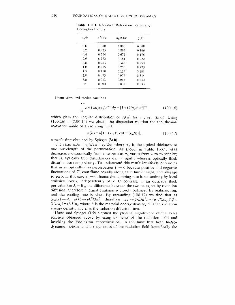
Table 100.1. Radiative Relaxation Rates andEddington Factors
K~,1k n(k)/u ~E(k)/1~ f(k)
0.0 1.000 1.000 0.0000.2 0.725 0,893 0.1060.4 0.524 0.676 0.1760.6 0.382 0.481 0.2220.8 0.283 0.342 0.2531.0 0.2J5 0.250 0.2731.5 0.118 0.129 0.3012.0 0.073 0.076 0.3145.0 0.013 0.0”13 0.330m 0.000 0.000 0.333
From standard tables one has
J“cos (/.L/iy/Ko)C -y dy = [l+(k/Ko)’~’]-’, (100.16)
o
which gives the angular distribution of 11(~) for a given (k/Ko). Using
(1 00.16) in (100.14) we obtain the dispersion relation for the thermalrelaxation mode of a radiating fluid:
n(k) = v[l –(KO/k) cot-] (KO/k)], (100.17)
a result first obtained by Spiegel (S18).The ratio KO/k = KoA/27r = rA/2T, where 7A is the optical thickness of
one wavelength of the perturbation. As shown in Table 100.1, n(k)decreases monotonically from u to zero as ~~ varies from zero to infinity;that is, optically thin disturbances damp rapidly whereas optically thickdisturbances damp slowly. To understand this result intuitively one notesthat in an optically thin perturbation II -+ O because positive and negativefluctuations of TI contribute equally along each line of sight, and averageto zero. In this case .TI-+ O, hence the damping rate is set entirely by localemission losses, independently of k. In contrast, in an optically thickperturbation J,= B,, the difference between the two being set by radiationdiffusion; therefore thermal emission is closely balanced by reabsorption,and the cooling rate is slow. By expanding (100.17) we find that as(Ko//c) + CXI, n(k) + uk2/3K~; therefore tm ~ 3K~/k2v ~ (pcUT,,/aRfi) x(l’/cA,,) = (2/E)t~ where Z is the material energy density, E is the radiationenergy density, and t~ is the radiation diffusion time.
Unno and Spiegel (U9) clarified the physical significance of the exactsolution obtained above by using moments of the radiation field andinvoking the Eddington approximation. In the 1im it that both hydro-dynamic motions and the dynamics of the radiation field (specifically the
RADIATING FLOWS 511
rate of change of the radiant energy density) can be ignored, the first law ofthermodynamics for the radiating fluid (96.9) yields an alternative energyequation:
pcU(dT/dt) = –V . F. (100.18)
It is important to remember the restrictive assumptions on which (1 00.18)is based. Next, making the Eddington approximation Kij = ~J i3ij and drop-
ping the time-dependent term in the radiation moment urn equation, weobtain an explicit expression for F [cf. (97.68)], by means of which we canrewrite (100.18) as
PCv(d~/dt) = V “ [(4 W/3K) VI]. (100.19)
The a.pproximations made here are the same as those used in the nonequi-librium diffusion approximation (cf. $97). Then substituting for J from(100.1) we have
Pcu(dT/dt) = V - {(1/3K) V[a~CT4+ (PC0/K)(dT/dt)]}, (100.20)
which describes the thermal behavior of a static radiating medium, in theEddington approximation, when time evolution of the radiation field isignored. Finally, linearizing (100.20) and using the fact that V7-0 = O(homogeneous medium) we find
(V2–3K2)(2T1/dt) =–VV2Tl, (100.21)
where v is defined by (IOO.1O)I.The essential physics emerges when we examine (100.21) in the opaque
and transparent regimes. In opaque material K/ -+ CD, where 1 is a charac-teristic length, and (100.21) limits to the diffusion equation
(dT1/dt) = (V/3K2) V2TI, (100.22)
which shows that radiative relaxation occurs on a characteristic time
scale ~ 3 K2i ‘/v, as found above. For transparent material K~-0 and(100.21) limits to Newton’s law of cooling
(dT, /dt) = –vT,, (100.23)
according to which the rate of cooling is linearly proportional to the size ofthe temperature fluctuation, and has a characteristic time scale tRR= 1/v.
Using a trial solution of the form (100.12) in (100.21) we recover(100. 13), but with the exact n(k) replaced by
?tE(k) = v/[l+3(K0/k)2]. (100.24)
Equation (100.24) has the same limiting behavior as (100.17) when(KO/k) -+ O and (KO/k) ~ ~, and, as shown in Table 100.1, provides areasonably good approximation in between.
When the effects of scattering are included, K. is replaced by (K + a). in
512 FOUNDATIONS OF RADIATION HYDRODYNAMICS
(100.19), hence (100.24) becomes
n~(k) = v/{1 +3[KO(K +cr)o/k2]}. (100.25)
From (1 00.25) one sees that for a given total opacity XO= (K+ a)o, increas-ing ~0 relative to K. afways increases the relaxation time. Indeed in the
limit of pure scattering (KO= O) we have the noteworthy result that n~(k) =~ = (), hence the medium behaves adiabatically, as one wou]d expect
because photons are conserved by a pure scattering process. When theeffects of energy exchange by thermal conduction are included (A6), (Dl),the relaxation rate becomes n = n,.~ + nCO.~,where n..n~ = (K/pcv) k2; hereK is the material thermal conductivity. Comparison of nr.~ and nCOn~showsthat radiation dominates only in long-wavelength disturbances, specificallywhen
k2< (16 UKKOT~/~)–3KO(K +U)O. (100.26)
From the fairly close agreement of n~ (k] and n(k) many authors haveconcluded that the Eddington approximation is valid for the perturbedradiation field in both the optically thick and thin limits. We can examinethis conclusion critically by calculating the Eddi ngton factor directly from(100.16), obtaining
J
1f(k) = L~’[1 + (k/KO)’/&’]-’ dp
IJ[1+ (fdKo)2~2]-’ d~ ~10027)
o 0
= (Ko/k)[l–(KO/k) cot-’ (KO/k)]/cot-’ (Ko/k).
Numerical values for f(k) are given in Table 100.1.. For optically thickdisturbances f ~ ~. But for optically thin disturbances f actually vanishes,
indicating that the perturbed radiation field is far from isotropic. In fact,the perturbed radiation field has a “pancake-shaped” distribution aroundthe normal to the plane of the disturbance, because in the plane (K = O),
~J(W)=B~, but as w ~ 1 (i.e., afong k) 11 -+ O because contributions from
the sinusoidal variation of B sum to zero when there is no attenuationalong the ray.
The real reason that n~ = n when Ko/k = O is not that the Eddingtonapproximation is valid in this limit, but rather that J, x (KO/k) ~ O in anoptically thin disturbance. Hence the absorption term KJ1 i n the energyequation vanishes, and the relaxation rate is set solely by the emission termK@I, which is independent of both k and f. Indeed, ret=i ng the deriva-tion of (~00.24), one finds that n~ = v when %/k = O no nlatter whatnumerical value is chosen for the closure ratio K/J; that is, the Eddingtonapproximation is irrelevant in the optically thin limit.
Spiegel’s formula for t~~ has been extensively applied in estimating theeffects of radiative cfalmping on waves in stellar atmospheres (cf. $$101 and102), But it is we]] to emphasize the restrictive assumptions on which it
rests: an infinite, grey, homogeneous medium in LTE; initial radiativeequilibrium: and no dynamics of either the matter or the radiation field. It
RADIATING FLOWS 513
entirely neglects boundary and nonlocal transport effects arising frominhomogeneities in the medium. The conditions under which the formula isknown to be valid are therefore very limited, and one must be careful notto misapply it.
As an example of the consequences of dropping some of the assumptionsmade in deriving (100.17), consider an ambient homogeneous, static, LTEmedium not initially in radiative equilibrium, but in a steady state underthe action of radiative energy exchange and a constant nonradiative (e.g.,magnetic) energy input (or loss) ~. Then
(dddt)o = &TKo(~o - ~.) + q = (), (100.28)
which implies JO # BO. (Such a state can be realized only for a finite
homogeneous medium, for otherwise .TOwould inevitably saturate to Be.)In this case we cannot omit the term 47rK, (J. – Bo) from the linearizedenergy equation, nor the term K1(~o — BO) from the Iinearized transfer
equation. Retracing the analysis we find that the effect is to replace BI inboth (100.6) and (100.8) by an equivalent source
(100.29)
and therefore u in (100.10) et seq. by
fi = (4mq/pco)[(aRc/m)T~ + (d in Ko/dT’)(& –Jo)]. (100.30)
When q >0, then Bo> JO, and the nonradiative energy input is balancedby excess emission. Then if (dKo/dT) >0, we have J > v, as one expectsbecause an increase in opacity produces an increased rate of emission. If,on the other hand, (dKO/d T) <0, so that the material radiates less efficientlyas it is heated, then J <v, and the relaxation time increases. Indeed if thesecond term in (100.30) is sufficiently negative, Z can become negative andan initial fluctuation will grow rather than decay; in this case the material isthermally unstable.
TIME-DEPENDENT RA D rATTON TRANSPORT
To extend the analysis we now allow for the finite propagation speed of
light and consider time-dependent radiation transport; we thereby allow theradiation field to have a dynamical character. As before, we assume nomaterial motions, which means that the material will respond only pas-sively to the radiation field. Intuitively we expect to find again a thermalrelaxation mode, but modified by the finite photon flight time tx = LP/c =
l/cK, and in addition, other new modes arising from the dynamical natureof the radiation field, including attenuated propagating radiation wavesthat correspond to the flow of radiation through an absorbing medium.
We adjoin the radiation energy and momenttum equations to the gasenergy equation and for steadily driven disturbances in an infinite homo-geneous medium derive a dispersion relation (which is independent ofglobal initial-boundary conditions) for the coupled set (A6), (Dl). TO close
514 FOUNDATIONS OF RADIATION HYDRODYNAMICS
the system of moments we invoke the Eddington approximation, encour-aged by the good results it gives in the quasi-static case.
For an infinite, homogeneous, grey, LTE medium initially in radiativeequilibrium the perturbation equations to be solved are (100.6) and
(l/CK)(d~l/dt)+ (l/K) (d~[/dX) = ~,–~1 (100.31)
and
(l/CK)(dH,/dt) +(l/3K)(dJJ/i)X) = –H,, (100.32)
where we noted that JO= BO and HO= O. Assuming plane-wave perturba-tions of the form @~= @eik’e-”[ we obtain the system
[
ntA– 1 —ikjK
)()
1 J,
–ik/3K ntk–l 0 H, =0 (100.33]
v o n—u B,
which has a nontrivial solution only if the determinant of coefficients iszero. From this requirement we obtain the dispersion relation
z3–(a+2)z2 +(a+p+l)z–ap =0, (100.34)
where zs ntk, a = vtA, and ~ = k2/3K2.
In general, (1 00.34) has either three real roots or one real root and two
conjugate complex roots. Given the roots A, (i = 1, 2, 3), one finds that theeigenvectors of the system have components
Vi(k) = (.~l, HI, B,)i =[1, (init~K/k)(ni– v–til)/(v–ni), v/(v–~)]x J,.
(100.35)
To gain physical insight we examine (~ 00.34) in various limiting cases.
Suppose first that tk -+ O, which implies that c ~ CO,hence quasi-staticradiation. We then recover (1 00.24) and thus have the same thermalrelaxation mode as before. We find
.T, = ~,/[g + (k2/3K2)] (100.36aj
and
H, = –(ik/3K)J1. (100.36b)
Note that J1--+Bl ancl H1-Oas~A ~~; and.T~--+O, H[~OasrA-+O;HI lags J, by T/2 as a function of x.
Next, suppose that v ~ O, which corresponds to material with infiniteheat capacity. Here the state of the matter is frozen, and a disturbance inthe radiating fluid can propagate only by radiation. The dispersion relationreduces to
2[(2–1)2+/3]=0, (100.37)
which yields roots z, = O and 22.3 = 1 + ik/& K. For n = O we can impose anarbitrary 5,, which does not decay in time; J, and H, are again given by
RADIATING FLOWS 515
(100.36), and merely represent the static adjustment of the radiation fieldto an imposed source perturbation (constant in time). The other two rootsare more interesting; we find BI = O and
H,= +J1/fi (100.38a)
where~~ ~ ~-t/tLeik[x&(c/>6)Ll (100.38b)
These are damped radiation waves propagating along the +x <axis with aphase and group speed cIJ~, attenuating in time at a given spatial position
on a time scale tA, or in space following a particular phase crest with aspatiaf scale (~ K)–’. These modes were rejected by previous authors(A6), (Dl), (F5), but are~in fact, legitimate modes in a radiating ffuid. Thepropagation speed is CIJ3 instead of c because we have used the Edding-ton approximation and therefcm-e obtain the telegrapher’s equation in theoptical] y thin limit instead of the exact radiation wave equation [cf. thediscussion following (97. 11 O)]. To obtain a better sojution we would needto calculate an accurate Ecidington factor for the time-dependent radiationfield.
Next consider a homogeneous disturbance (k= O). From (1 00.33) we findthe dispersion relation
Z(z–l)[z–(a+l)]=o (100.39)
which has roots Z1 = O, Zz = 1, ancl Z3 = a T 1. For the nondecaying modenl = O we find that .J~= B ~ and 111= O. Here we have merely reached a newequilibrium in the radiation field by making identical, constant changes in .1and B; HI is zero by symmetry. For the root n2ri = 1 we find that.T1= I?l = O, whereas HL is arbitrary. Thus we may apply any nonzeroperturbation in the specific intensity of the form II(w) = ZaiPi(~) as long asaO = a2 = O, which imp] ies that J, = K1 = O (Eddington approximation); aland a, for i a 3 may be arbitrary. Alternatively we may impose anazimuthal an isotropy such that J, and K, are zero (F5). Here we have anisotropization mode, in which an initial angular anisotropy of the radiationfielcl is removed by absorption and isotropic re-emission on a radiation-flowtime scale t~; the process is analogous to the establishment of an isotropicvelocity distribution function for material particles in a deflection time tD(cf. $1 O). Finally, for the root n,= v + t:’ we find .J1 = –B1/vt,, which yieldsexact energy conservation in the linearized gas energy equation, and
Ifl = O. Here we have an exchange mode in which a given amount of energyis removed from the radiation field and temporarily deposited in thematerial (or vice versa) thus conserving the total fluid energy, but destroy-ing radiative equilibrium. The disturbance decays back to equil ibri urn at arate even faster than the relaxation rate of a transparent disturbancebecause we have simultaneously increased B (hence the emissivity) anddecreased .J (hence the rate of absorption), or vice versa, which results in a

516 FOUNDATIONS OF RADIATION HYDRODYNAMICS
larger temperature imbalance (hence relaxation rate) than in an optically
thin disturbance where B is altered but the ambient .TOis unperturbed.Consider next the opaque h-nit, ~<< 1, where (100.34) yields three real
roots. We find that to first order in ~ the smallest root of (100.34) is
nl(k)= v(k2/3K2)/(1 * Vti), (300.40)
which is just the thermal relaxation mode, but with an effective relaxation
rate v/(1 + zll). The decreased relaxation rate is what one would expectintuitively because the radiation now takes a finite time to flow. In thismode J, and B] always have the same sign. For ~<< 1, J, and B., are nearlyequal and \HI I<<I.JII; and .TIe B, while H, + O when k ~ 0. Theisotropization-mode root in the limit of small ~ is
n2(k) = v{l – [(k2/3K2)(ut~ – l)/vtk]}. (300.41)
Again we have both IJII <<IHII and IB,]<< IHII. Finally, the exchange-moderoot in the limit of small ~ is
rzq(k) = v + t~’ –[(k2/3Kz)/vtf(l + utA)]. (100.42)
In this mode J, and B, always have opposite signs, and 111 is small and 90°out of phase with .TI.
Finally, consider the transparent limit /3~ ~. We find that (100.34) hasone real root
n, (m)== L’ (100.43)
and two complex roots
n2,3(~) = CK * ick/&. (100.44)
The real root corresponds to a pure damped disturbance; as we will shortlysee, the mode by which it decays depends on the value of a. The complexroots correspond to two damped radiation waves propagating with phaseand group speed c/N@. In these modes the sign parity of ~, relative to 131 isopposite to that in the surviving mode corresponding to n,. This fact andthe conjugate relation of the complex roots guarantees that with the threemodes we can always synthesize an imposed perturbation in which .TJ andBI have arbitrary relative amplitude and phase.
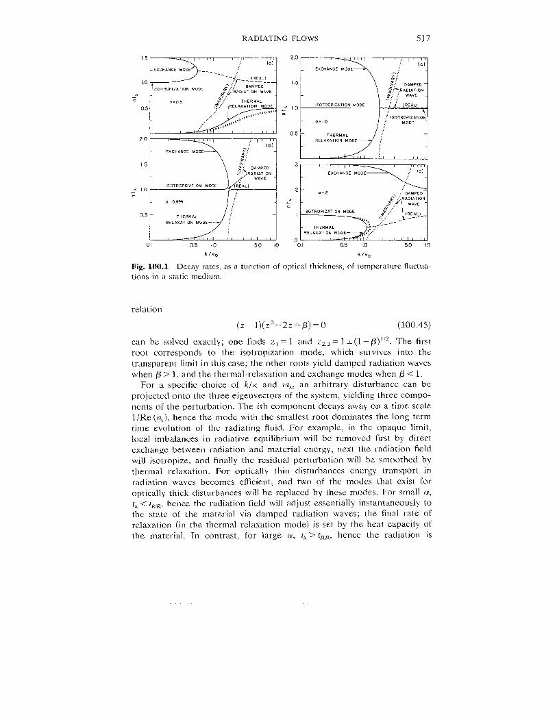
The analytical results discussed above are represented in Figure 100.1,which shows n(k) obtained from numerical solutions of (100.34). Foroptically thick disturbances we always find three real roots, correspondingto the exchange, isotropization, and thermal-relaxation modes. For smalloptical thickness we always fincl one real root and two complex roots
correspond ng to damped radiation waves. When a <1 the real rootcorresponds to the thermal relaxation mode; when a >1 it corresponds tothe exchange mode. The connectivity of the various branches changesabruptly at a = 1, as illustrated. For the special case a = 1 the dispersion
RADIATING FLOWS 517
15
P:j
(0)EXCHANGE MOOE -----,.:
Lo
ISOTROPIZATION MODE
:--?&!f;:L-
(? : RADIATION WAVE
z
““”’e’:’
2.0 I(c)
ExCHANGE MODE
}>-,,::/
1.55:LRAD1bT,oN
L, / ;~:::’ -
3;~,,
~loISOTROPIZATION MODE
z f! lSOTROPIZATlON
05 – THERMAL
RELAXATION MODE
t
:0-. I
, ymll;:t. ,
“SW( ,,,,,,,
3
CXCHANGE MODE
2 -,,.’
,7.2
.
z
ISOTROPIZATION MODEI
RELAXATION MODE
o0, I 05 1.0 5,0 10 0.I 0,5 ILO 5.0 !o
k {<0 k /<.
Fig. 100.1 Decay rates, as a function of optical thickness, of temperature fluctua-tions in a static medium.
relation
(z-l) (z2-2z+p)=o (100.45)
can be solvecl exactly; one finch Z1 = 1 anct 22,s = 1 *(1 – B)J’2. The firstroot corresponds to the isotropization mode, which survives into thetransparent limit in this case; the other roots yield damped radiation waveswhen /3 >1, and the thermal-relaxation and exchange modes when /3 <1.
For a specific choice of ldr< and vt~, an arbitrary disturbance can be
projected onto the three eigenvectors of the system, yielding three compo-nents of the perturbation. The ith component decays away on a time scale1/Re (nt), hence the mode wit!h the smallest root dominates the long-termtime evolution of the radiating fluid. For example, in the opaque limit,local imbalances in radiative equilibrium will be removed first by directexchange between radiation and material energy, next the radiation fieldwill isotropize, and finally the residual perturbation will be smoothed by
thermal relaxation. For optically thin disturbances energy transport inradiation waves becomes eflicient, and two of the modes that exist foroptically thick disturbances will be replaced by these modes. For small a,ti< tR[<,hence the radiation field will adjust essentially instantaneously to
the stale of the material via damped radiation wa~’es; the final rate ofrelaxation (in the thermal relaxation mode) is set by the heat capacity ofthe material. In contrast, for large a, tk > tJZ17,hence the radiation is
518 FOUNDATIONS OF RADIATION HYDRODYNAMICS
essentially “frozen” and the material adjusts rapidly to the local radiationfield via the exchange mode; final global smoothing of the initial distur-
bance then proceeds via damped radiation waves.All of the results discussed above are based on the Eddington approxi-
mation, which, as we saw from (1 00.27), breaks down for optically thindisturbances. Delache and Froeschle (Dl), (F5) attempted instead to findan exact sol ut ion. They obtained a dispersion relation that yields only oneor two real roots, and concluded that the complex roots of (100.34) mustbe rejected, thereby discarding the damped radiation waves. However,their solution encounters a severe difficulty in the optically thin regimebecause they find only one mode, which has the unacceptable implicationthat one is not free to impose an arbitrary initial disturbance, but only onewith the correct relationship (both in sign and relative size) between .TI andB ~. This lack of a complete set of modes indicates a deficiency in theanalysis.
In fact, the formal solution in (Dl) is invalid when ntk 21 becauseinitial-boundary conditions are not accounted for correctly [cf. (79.35)].The mathematical symptom is that a certain integral diverges unlessnt~<1 ; physically the divergence occurs because the integral is swampedby an exponentially divergent source when the integration is extended tot ~ –~ instead of being truncated at t = O (the instant when the initial
perturbation was imposed). The solution in (F5) suffers from a similarproblem. Furthermore, when correct limits are applied in the formalsolution it is no longer possible to use a separable solution of the form(1 00.1.2). Thus the proposed “exact” solution appears to have only limitedapplicability y.
In our opinion the Eddington approximation should always yield resultsthat are at least qualitatively correct. For example, suppose ntl <1. Herewe expect the Eddington approximation to be valid in the opaque limit,and to become irrelevant in the transparent limit. As a test we replace thefactor ~ in (100.32) to (100.34) with the quasi-static f(k) given by (100.27).As shown in Figure 100.1 we find little change in the modes with nt, <”1.The same remark holds for modes with nt~ s 1, but in this case we cannotguarantee that (100.27) is valid. However, we know that for a mode withntL>1 the material equilibrates to the local radiation field via isotropicemission and absorption processes on a time scale shorter than thatrequired for radiation to flow to (or from) adjacent regions. Therefore if weassume (legitimately) that the initial radiation perturbation is isotropic, wecan argue that it must remain isotropic during the lifetinle of the mode,hence that the Eddington approximation will apply. Similarly, for ntA= 1
the effect of the isotropization mode is to isotropize an initially anisotropicdistribution. Likewise the damped radiation modes will propagate an initialisotropic disturbance isotropically. In all cases the Eddi ngton approxima-tion appears reasonable.
The radiative relaxation of a medium comprising non-LTE two-level
RADIATING FLOWS 519
atoms, radiation, and an ambient LTE gas is discussed in (L7), (F5), and(F6). Appropriate rate equations are adjoined to the gas energy andradiation transport equations. The resulting dispersion relation is morecomplicated and yields a richer spectrum of modes, which now depend oncharacteristic time scales governing the kinetics of statistical equilibrium(e.g., radiative and collisional rates) in addition to the parameters enteringin the cases discussed above.
Virtually all astrophysical discussions of the radiative damping of tem-perature fluctuations and/or waves are based on (100.17) or (100.24), andthus ignore the time dependence of the radiation field. This simplification isusually justified because the dynamical time scales of many astrophysicalphenomena are enormously longer than a photon flight time, hence theradiation field is indeed quasi-static and the fast exchange, isotropization,and damped-radiation-wave rmodes are of little interest. A similar situationis encountered in fluid dynamics where in order to follow the evolution offlow phenomena having long time scales, one can make the anelasticapproximation and adopt modified equations of hydrodynamics that sup-press sound waves, thereby filtering out variations on short time scales thatotherwise are a nuisance computation ally.
THERMAL RESPONSE OF THE SOUR P.TMOS PH ERE
In attempting to apply (100.17) to estimate the radiative relaxation time oftemperature fluctuations (or waves) in a stellar atmosphere, one mustaccount for two important effects: (1) the variation of material properties,hence v, with height, and (2) the presence of an open boundary.
Estimates of the relaxation time for an optically thin disturbance, tRR(~),
have been made by several authors [e.g., (B6, 326), (S17), (S24), (U3)]using realistic model solar atmospheres. Allowing for continuum opacitiesonly, one finds that t~~(m) in the photosphere (~COn,= 1) is about 1 s, andrises rapidly with height, reaching a maximum of about 800s at about700 km above the photosphere. At greater heights the relaxation timebegins to drop because of rising temperature, then passes through asecondary maximum as hyclrogen ionizes, and finally plunges sharply.These results are modified drastically when radiative losses in spectral linesare included (G5); one then finds that tRR(o$ rises to about 500 s justabove the temperature minimum, then falls to only 90 s in the mid-
chromosphere where line losses a~e large, before rising again to about400s when hydrogen ionizes. Unfortunately it is difficult to allow properlyfor self-absorption in the spectral lines, hence to estimate accurately theirnet cooling rate, and the line-loss term is uncertain by at least a factor of 2.
Below rCO.,= 1, tR1<(~) drops rapidly as K rises sharply. But for adisturbance of finite wavenumber k, the increase of ~,1 with increasing K
implies that tRR(k) increases rapidly, in accordance with (100. 17). Ulti-mately, tRR(k) becomes so large that a time-periodic disturbance behavesessentially adiabatically (wtRR >>1). Because the atmosphere has an open
520 FOUNDATIONS OF RADIATION HYDRODYNAMICS
boundary the effective relaxation rate of a disturbance depends on itsoptical depth ~ in the atmosphere, as well as on 7A. Thus a horizontalperturbation will relax by horizontal radiative exchange between crests andtroughs if ~A<<T, but if ~A>>~ it relaxes more efficiently as a result ofvertical radiative losses through the open boundary. Ulrich (U8) suggestedthat in calculating tRR from (1.00.17) we use an effective optical thicknessgiven by
In physical terms (100.46) gives the harmonic mean of the number ofabsorption a photon requires to cross one wavelength of the disturbance,and the number to escape from the atmosphere. For a vertical disturbanceone can use (100.46) or simply choose ~ef = min (~, 7A). In an exponentialatmosphere ~,, :7 = A: H, hence 7A sets the relaxation rate only for short-wavelength disturbances (or for long-wavelength disturbances deep in theenvelope where H becomes large).
The thermal response of the solar atmosphere to periodic time variationsof the radiative flux incident from below is examined numerically in (W5).The atmosphere is assumed to be motionless, but allowance is made for aninhomogeneous vertical structure. A sinusoidal variation with a 10 percentamplitude in the radiative flux is imposed at the lower boundary. Initialtransients (the subjects of study elsewhere in this section) are allowed todie out, and the final periodic solution driven by the boundary condition isobtained. From the numerical results one finds that (1) the amplitude ofthe temperature fluctuation decreases with increasing height, (2) there is aphase lag between the imposed flux and the temperature response, (3) thelag increases with height, and (4) the lag is an increasing fraction of aperiod as the period decreases.
To understand these results qualitatively, consider the optically thin part
of the atmosphere, and assume that
7-(2, t)= 2-.[1 +f(z)ei-”] (100.47)
and
J(t) = -TO(l+ &e’”’), (100.48)
where TO is a suitable average and JO = 130= ~~T~/m. The perturbation s isconstant because the region considered is optically thin. The linearizedenergy equation then reduces to
io.$(z) = (4 UR(K)T~/CU)[C –4&(z)]. (100.49)
In general both E and f are complex, but we can choose the timecoordinate so that s is real, whence we have
& = –~1/&dJ/(@’+ ZJ2) (1.00.50a)
and[R/[, = –v/m. (100.50b)

RADIATING FLOWS 521
Therefore
1.5(Z) I = Mz)d[@2+ J’2(Z)J”2 (100.51a)
and
c$(z) = –tan-’ [@/v(z)].
Here ~ is the phase angle between J, and T,;lags .T. In the high-frequency limit, o/v - ~,
Igl -+ +v&/co+ o
and
~+.22’
(100.51b)
negative @ indicates that T
(100.52a)
(100.52b]
so the thermal response lags the input by 90° and its amplitude vanishes. Inthe low-frequency limit, ~/v e O,
l~l~~E (100.53a)
and
@+o, (100.53b)
hence the atmosphere passes through a series of quasi-equilibria withvanishing phase lag. Equatic)n (100.5 la) shows that the phase lag mustincrease with height because v decreases outward through the photo-sphere; the approximate results given by (100.51) are in good agreementwith the numerical results.
The radiative relaxation of a two-dimensional checkerboard distributionof temperature and density fluctuations simulating a hydrodynamic modelof convection cells in the solar atmosphere is discussed in (L8). Therelaxation rate is found to depend on the cell size, the size of the velocityfield, and the amplitude of the initial temperature fluctuation.
101. Propagation of Acoustic Waves in a Radiating Fluid
In this section we examine the effects of radiation on acoustic wavespropagating in an infinite, homogeneous medium in LTE, initially in
radiative equilibrium. We first consider wave damping by radiative energyexchange, which is generally very efficient, especially near boundary sur-faces (e.g., the solar photosphere) where radiative relaxation times are veryshort compared to typical wave periods. By comparison, wave damping byviscosity and thermal conduction is negligible in most situations of astro-physical interest. We treat the spatial damping of driven harmonic distur-bances (i.e., real w and complex k) as opposed to the time decay of atransient initial disturbance (i.e., real k and complex co). We then considerthe more fundamental role played by radiation through its contributions tothe total energy density and pressure in the fluid; we find that radiation can

522 FOUNDATIONS OF RADIATION HYDRODYNAMICS
radically alter the dynamical properties of wave modes in the fluid. Finally,we consider briefly the effects of radiation forces on acoustic waves.
NEWTONIANCOOLING (OmIcALLy THIN PERTUR13A-IIONS)
Consider first an optical] y thin disturbance in which radiative energyexchange is adequately described by the Newtonian cooling approximation(S16), (S25). We assume that the radiation field is quasi-static and ignorethe dynamical behavior of the radiation component of the radiating fluid.From (1 00.23) the net heat input to the gas is then
(Dq/Dt) = –pcov-r, (101.1)
where v is given by (100.10). Using (101 .1) in (52.19) we can write the gasenergy equation as
(Dp/Dt) -u2(Dp/Dt)=–16(r, - l)a~KOT~(T,/TO). (101.2)
For the special case of a perfect gas with constant specific heats, we canrewrite the right-hand side of (101 .2) in a more convenient form. For such~gasr~=y,(y—~)~u ‘R~a 2 = -YP/P, and T1/To = (PJPOI –(PI/Po), and thelinearized version of (1 O1.2) reduces to
(dpl/dt) = a2(@Jdt) + v - (a’ Vpo - Vpo) – (a2Po/ytRR)[(pI /po) - (pl/P.)l,
(~ol.3)
where for brevity we write tRR= tm (CO)= V–l.Note in passing that for anionizing gas the linearized energy equation is
(dpl/dt) = a2(dpl/dt)+v” (rX2Vp0-VPo)– a2po[a2(pl/po) –al(pl/po)l,
(101.4)
where, from (54.84a), CYland a2 for a pure hydrogen gas are
al =[16(r3– l)crRKoT$/r LpO]/{l +~x(l – x)[~+(&r/kT)]} (101.$
and
cK2=[l-E;x (l-x)]a L. (101.6)
For a homogeneous medium the gradient terms in (101 .3) vanish, hencethe dynamics of a radiatively damped acoustic wave is determined (in theNewtonian cooling approximation) by
(ap,/dt)=pQv” v,, (101.7)
Po(fN’1/at) = –vPI, (101.8)
and
(dpl/i3t) - a2(@L/dt) = -(a2po/7tRR)[(p1 /pO) - (dpo)]. (101 .9)
Taking (d2/dt2)of (101 .9) and using (48.6), which follows from (10~ .7) and
RADIATING FLOWS
(101 .8), we obtain the wave equation
{[(d’/dt2) – cl’ Vz](d/LJt)+ t~~[(d2/dt’) -
For plane waves (101 .10) yields the clispersi
523
a2/y) V2]}p, = O. (101.10)
,n relation
( )[~2= $ (1+ ‘y@’t&) – i(y – I)@tR.
1 (101.11)az 1 + y~@3& ‘
Because k is complex we find damped progressive waves varying ase i(a[—k Rx)e —lcrx
In the high-frequency limit, wt~~ >>1, and
k = (@/a){~ – z[~(Y – 1)/Y@tKR]}> (101.12)
which corresponds to acoustic waves traveling with the adiabatic sound
speed, having a characteristic damping length
L== [27/(7 – l)]atRR. (101.13)
Note that L/A- o&~ >}1, hence in the limit of high frequencies and/orlong damping times, acoustic waves behave essentially adiabatically and
suffer only a small damping per cycle. Note, however, that (101.13) showsthat the geometrical distance over which the wave damps can be madearbitrarily small by making the relaxation time sufflcientl y short; in thissense high-frequency waves can be heavily damped.
In the low-frequency limit, dRL<cc1,and
k = (co/a-,.)[1 – i~(y – l)~t~~], (101.14)
where a.-,. is the isothermal sound speed a/-y 1!2. We now have acousticwaves traveling with speed aT, with a damping length
L = [2/(7 – 1)]a-rt,<~/(oN~~)2, (101.15)
which implies that L/A– (@tM. )“ >>1. Thus according to Newtonian cool-
ing theory, in the limit of low frecluencies and/or short radiative relaxationtimes radiative exchange obliterates temperature fluctuations in the gas,and acoustic waves propagate isothermally with negligible spatial damping.
For arbitrary @tRR one solves (101.10) numerically. As shown in Figure101.1, the phase speed vu = o.dk~ rises abruptly from a-r to a nearcotm = 1. At the same time, the damping length L/A= lk~/2wkr\ passesthrough a minimum. Indeed, near cot~~ – 1, L/A= 1, so these waves decay
after traveling only a few wavelengths.It must be emphasized that all of the above results apply only for
optically thin disturbances, ~/k <<1, A/& <<1. The significance of this
remark will become clear shortly.
.

524 FOUNDAHONS OF RADIATION HYDRODYNAM [CS
100
10
I I I I I 1 1 1 I I I I L
1.0 ~ I I [ I I I I I
A 0.9 –<L
3 0.8 –
0.7 t I I I I I I 1 I I I-3 -2 -1 0 I 23
log d~R
Fig. 101.1 Damping length and phase speed of acoustic mode in Newtoniancooling approximation.
EQUrLJ13RIUM DIFFUSJON (OFWCALLY THICK DKTURBANC13S)
In extremely opaque material (e.g., inside a star), radiation comes intothermal equilibrium with the matter, and energy exchange proceeds bydiffusion; in this regime radiation can have important dynamical effects onwave propagation. In treating the radiation field we can apply the equilib-rium diffusion approximation provided that the disturbance is sufficientlyoptically thick, that is, that K/k >>1.,and A/Ap >>1.
The dynamical equations for a radiating fluid in the equilibrium diffusionregime were derived in $97. From (97.5) and (97.6) the momentumequation is
p (Dv/Dt) = –Vp (101.16)
and the energy equation is
P{(W~~) + FID(HP)i~~l} = v . (~ VT). (101.17)
RADIATING FLOWS 525
Here p, Z, and ~ are the total pressure, energy density, and conductivity ofthe fluid:
~ = Pw,+ Pr,~ = PRT+ iaRT4 = (1 + a)pRrr, (101.1.8)
.z = cc,,, + (a~T4/p) = 2RT+ (a~T4/p), (1.01.19)
and
R = K,,.,”,:,, + I’c,.a., (101.20)
where K,z,c{is defined by (97.3). Using (52.19) we rewrite (1 OI.1.7) as
(Dfj/Dt)-a2(Dp/Dt) = (17-I)V” (~VT) (101.21)
where
a2=171p/p = (1 +~)rl(ag,L,/7), (101.22)
and rq and rl are given by (70. J 8) and (70.22).For a small disturbance we linearize these equations. The linearized
continuity and momentum equations are the same as (101.7) and (101..8)
(with p, replaced by ~,), and therefore again yield (48.6). The linearizedenergy equation is
(ap,/at)– a2(dpJdt) = (r, - l)I? V*T,. (101.23)
We can eliminate T1 in favor of ~, and PI by means of the linearizedequation of state
T,/TO= [(l+ Ix)(~I/Do) ‘(PI/Po)l/(1+4~) (101.24)
Thus using (101.24) in (101 .23) and making use of (70.16), (70.18), and(70.22) we find
(tq3,/at)- a’(dddt) = rx[v’pl- (a*/r)V2p,] (101.25)
where we defined an effective r as
r=(l +a)r, (101.26)
and the thermal diffusivity is
x = K/pocv. (101.27)
With these definitions (101.25) is formally identical to (51.5) for a heat-
conducting gas. Taking (d2/dt2)of (101.25) and using (48.6) to eliminate PIwe obtain the wave equation
{[(a2/dt2)-a’ V2](d/dt) -17x[(d2/dt2)- (a2/I’)V’] V2}@l= O. (101.28)
For a plane wave (101 .28) yields the dispersion relation
(ak/co)4 -[r - i(a2/Xw)l(ak/w)2– i(a2/xO) = 0, (101..29)
which is quadratic in (ak/co)2, and contains two dimensionless numbers: 1-and Xco/a2. This dispersion relation is formally identical to (51.16) for a
526 FOUNDATIONS OF RADIATION Hydrodynamics
thermally conducting inviscid material gas. Hence we obtain the samemodes and physical interpretation as before: an adiabatic (isothermal)radiation-modified acoustic wave, and a slow (fast) radiation-diffusion wavein the low (high) frequency limits, respectively. These waves have the samepropagation characteristics as described in $51 (cf. Figures 51.1 and 51.2);only the thermodynamic parameters (x, 17,a) differ from their earlierdefinitions. Thus in the equilibrium diffusion regime radiation is an in-separable part of the radiating fluid, with photons behaving dynamicallylike “honorary material particles”. *
It should be noted that as a ~ ~, 17, a, and CP diverge, but this is anartifact of having ignored the rest energy of the ffuid in our analysis [cf.
(48.32) and (70.27) for a]. The divergence occurs only at extremely hightemperatures where relativistic effects are major and a relativistic anaJysisis required. In contrast, it follows from (101.22) and (101.26) that a2/r =
(a%)U,,, hence the phase speed of the isothermal acoustic wave depends ongas properties only.
The analysis can be extended to include the effects of electromagneticfields in an ionized plasma; see (PI, $8.2).
TIM13-TNDEPENDEN-rTRANSPORT (EDDrNGTONAPPROXIMAr[ON)
The Newtonian cooling and equilibrium diffusion approximations conflictwith each other in that they predict opposite variations of the propagationspeed (i.e., adiabatic versus isothermal) of the acoustic mode in going fromlow to high frequency. This contradiction arises because each schemebreaks down in one or the other limit. Thus at a sufficiently low frequencythe wavelength of a disturbance is so long that it becomes optically thick(no matter how transparent the material), and the Newtonian coolingapproximation no longer applies. Conversely, at very high frequencies thewavelength of a disturbance becomes so small that it is optically thin (nomatter how opaque the material) and the difision approximation is nolonger valid because a photon mean free path exceeds the characteristicspatial scale of gradients in the disturbance (recall the discussion of fluxlimiting in $97j.
These considerations show that it is imperative to account for transporteffects arising from finite photon mean free paths in the disturbance. Ourqualitative expectation based on the diffusion approximation is that wavesshould be adiabatic at very low frequencies, and become isothermal abovesome critical frequency; but then at some sufficiently high frequency thewaves should again become adiabatic, as predicted by the Newtoniancooling approximation. Precisely this behavior was found by Stein and
Spiegel (S23) in their analysis of the time decay of an initial disturbance,allowing for transport effects (but ignoring the time dependence anddynamical behavior of the radiation field). in keeping with the rest of the
* we are indebted to Dr. J. I. Castor for this felicitous exmssion
RADIATING FLOWS 527
discussion of this section, we consider instead the spatial damping of adriven disturbance along the lines explored by Vincenti and Baldwin (V6),(V7, $$12.5-12.8).
The dynamical behavior of the material is governed by the continuityequation, the material momentum equation
p(Dv/Dt) = –Vp, (101.30)
and the gas energy equation
(@/Dt)– a2(Dp/Dt) = 47r(y– 1) K(F13). (101.31)
Here p refers to the gas pressure only, and a2 = yp/p. In (101..30) we haveneglected the radiation force on the material.
We assume that the radiation field is quasi-static and make the Edding-ton approximation. The radiation energy equation is then
(d~/dX)=K(~-~) (101.32)
and the radiation momentum equation is
~(~~/~~) = ‘K~ (101 .33)
Equations (10 ~.32) and (101.33) provide a significant improvement overthe Newtonian cooling approximation because they apply in both theoptically thick and thin limits. They are also an improvement over equilib-rium diffusion because they discriminate between J and 1?, which is crucialwhen the disturbance becomes optically thin. However they sacrifice some
of the logical consistency inherent in the equilibrium diffusion analysisbecause they ignore the dynamics of the radiation field; we will remedythat flaw later.
In linearizing the radiation equations we note that JO= BO and HO= O,and introduce nondimensional radiation variables j, = -f~/f30, h 1~ H~/BO,
and l?l/Bo = 4T1/To = 461. Combining the linearized forms of (101.32) and(101.33) we have
(3 K2)-L(d2j,/dX2) ‘jl ‘401. (101.34)
In linearizing the continuity and material momentum and energy equationswe use a velocity potential U1= (~~, /3x) which implies that (dpl/dt) =
–po(d2d1/dx2) and, from (101.30), PI = –po(&$l/r3t). Using these expres-sions in the linearized gas energy equation we find
(d2{$1/at2] – a2(tt2&/~x2) = (4a3K/Bo)(40, ‘j,) (101.35)
~,here Bo is the Boltzmann number obtained by setting the characteristic
flow speed equal to the sound speed:
Bo - pOcUa/m~T~. (101 .36)
Similarly the linearized equation of state for the material can be written
(r12+,/dt2)– (a2/y)(d24,/dx2) +(a2/7)(dol/at) = 0. (101.37)
528 FOUNDATIONS OF RADIATION HYDRODYNAMICS
For a plane wave (101 .34), (101 .35), and (101.37) imply
[
o –4
)(1
1 +(k2/3K2) ~,
(a’k’/co’) – y ia’lw o e, = O. (101.38)
(a’k’/w’) -1 –16a3K/C02B0 4a3K/a2B0 j]
Setting the determinant of (101.38) equal to zero we obtain the dispersionrelation
[1 - Z(167a/BO)](ak/LO) 4-[1 -3T~– i(16y~a/Bo)](ak/co)2- 37:= O.
(101.39)
Here
T. = CLK/@ = TAIZ’TT, (101.40)
where 7A is the optical thickness of one wavelength of a disturbance offrequency o traveling with the adiabatic sound speed a. Like (101 .29),(101 .39) is quadratic in (a’k’/co’), hence we again get two distinct wavemodes. One is a radiation-modified acoustic wave; the other is a nonequi-libriurn radiation diffusion wave analogous to a thermal wave.
The importance of radiation to the behavior of these waves is measured
by Bo. In the limit Bo e ~ radiative energy exchange with the materialceases. In this special case the dispersion relation factors into
[(ak/co)2- l][(ak/~)2+ 37:] = O, (101.41]
and we obtain (1) an undamped adiabatic acoustic wave in which 01 and VIare related by (48.24b), and .~l and B] are related by (100.36), and (2) aradiation-field pert urbation j, decaying as exp (—W KX) [as one expects forthe Eddington approximation, cf. (83.7)], while ~1 = 01 =0.
Solving (1 O1.39) for ~a <<1 (small optical thickness and/or high fre-quency) we find a weakly damped acoustic wave with
k = (du)[l – i87u(y – 1)/Be], (101.42)
which implies that Vp= a and L/.A = [BO/167rTa(y – I)] >>1, and a fast,strongly damped radiation diffusion wave with
which implies that vpla = Bo/8& yr~ and L = I /w@K or L/A = 4yr./7TBo.Note that as ~. e O, the clamping length for the acoustic mode becomesinfinite, whereas the diffusion mode has an infinite phase speed and a fixedgeometrical damping length, while L/A ~ O. The infinite propagation speedof the diffusion mode reflects the failure of the quasi-static radiationequations to provide flux limiting in opticafly thin material.
For 7.>>1 (i.e., large optical thickness and/or low frequency) we find adamped acoustic wave with
k =(w/a)[l – i8(y– 1)/37.Be], (101 .44)

RADIATING FLOWS 529
which implies that V. = a and L/A = [37a Bo/16w(y – ])]>> 1, and a slow,heavily damped diffusion wave with
k== (co/a) (3~.Bo/32)’’2(l – i), (101.45)
which implies that vp/a = (32/3 ~aBo) 1’2<<1 and L/A ==l/27r. The predictionby (101 .44) that the acoustic-mode speed always equals the material soundspeed independent of the radiation energy density (i. e., Bo) is in contradic-tion with equilibrium cliffusion theory (which is valid when ~a >>1) andreflects the failure of (101 .32) and (101 .33) to account for the dynamics ofthe radiation field.
In general, (101 .39) must be solved numerically. Results for variousvalues of Bo are shown in Figures 101.2 and 101.3. For context, Bo is of
order 10 in the solar photosphere and at the Sun’s center, 10–2 at thecenter of an O-star, 10-5 in an X-ray source, and 10–lQ or smaller in asolar flare. Figure 101.2 shows that the acoustic mode is indeed adiabaticat high and low frequencies, and is isothermal over a range approximatelyinversely proportional to Bo. Furthermore, we see that the damping lengthis large when the phase speed is constant, but drops shqlY where VPmakes a transition between a and al-. Figure 101.3 shows that v. in the
1000
100
10
I
E
FI I I I I I I I I I I
–5–4-3–,2-lo Iz 345
log To
Fig. 101.2 Damping length and phase speed of acoustic nlode for quasi-staticradiation field, allowing for transport effects.
.. .
530 FOUNDATIONS OF RADIATION HYDRODYNAMICS
100
,~-1
< 10-z-r
,(3-3
L I I
. . .
.“
I I I 1 I I I I I I I
,02
10
~zlb
10-’
,.-2,“
-3 -2 -i o I 23
log To
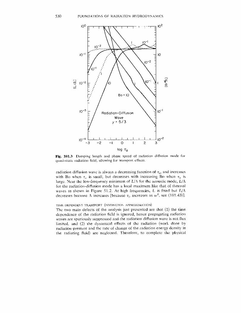
Fig. 101.3 Damping length and phase speed of radiation diffusion mode forquasi-static radiation field, allowing for transport effects.
radiation difision wave is always a decreasing function of T., and increaseswith Bo when T. is small, but decreases with increasing Bo when T. islarge. Near the low-frequency minimum of L/A for the acoustic mode, L/Afor the radiation-diffusion mode has a local maximum like that of thermalwaves as shown in Figure 51.2. At high frequencies, L is fixed but LIAdecreases because A increases [because v, increases as @z, see (101 .43)].
‘rrME-DEPENDmrr TRANsPoR-r (EDDINCWON APPROXrMATlON)
The two main defects of the analysis just presented are that (1) the timedependence of the radiation field is ignored, hence propagating radiationwaves are spuriously suppressed and the radiation diffusion wave is not fluxlimited, and (2) the dynamical effects of the radiation (work done byradiation pressure and the rate of change of the radiation energy density inthe radiating fluid) are neglected. Therefore, to complete the physical
RADIATING FLOWS 531
picture we account for these phenomena by including the radiation pres-
sure gradient in the material momentum equation
p(Dv/Dt) = –Vp –VP (101.46)
and by using the Lagrangean radiation energy and momentum equations
c-’(DJ/Dt) - (4J3cp)(Dp/Dt) + (d~/dX) = K(B -J) (101.47)
and
c-l(DH/Dt) +~(dJ/dX) = ‘KH. (101.48)
The gas-energy equation (10 1.31) remains the same as before.In (101.47) and (101.48), we have made the Eddington approximation,
so in (101.46) P = *E = (47r/3c).I In (101.46) we have neglected the timederivative of H, which is permissible because that term is at most O(a/c)
relative to VP, which in turn produces terms that are only O(a/c) relativeto the dominant terms in the dispersion relation (except at very smallBoltzman n numbers).
The linearized continuity ecluation again yields (dpl/~t) = –pO(d2&/~x2),
while the linearized material momentum equation is
Po(~u@) = “(~P ,/Jx) – (47Tf30/3c)(dj1 /dx)) (101.49)
which implies
P ~= ‘Po(MJdt) – (4d30/3c)j~. (101.50)
Using these expressions in the linearized gas-energy equation and materialequation of state we find
(a2@l/dt2) - a2(d2C$,/dX2) + [4a 3/3c(y - l)Bo](dj,/dt) = (4a3K/BO)(401 - j,)
(101.51)and
(d2&/dt’) - (a’/y)(d’@,/dx’) + (a’/’y)(a6Jdt)(101.52)
+ [4a3/3c(y – l) Bo](djl/dt) = O.
For a p~ane wave, (101.51) and (101.52) become
(azk’-co’)+, –(16a3K/BO)01 +(4a3K/Bo)[l+ i~(y - l)-’ ~~’]jl = O,
(101.53)and
(a’k’-yco’)+, + ia’dl+ (4a3K/BO)[i~Y(Y - l)-’ ~;”’]jl = O. (101.54)
By analogy with (101.40) we have defined
Tc = CK]O+ (101.55)
the optical thickness associated with a disturbance of frequency o travelingat the speed of light (not sound). Notice that ~C: ~. = c : a, hence in anacoustic wave of any appreciable optical thickness ~C}>1.
532 FOUNDATIONS OF RADIATION HYDRODYNAMICS
The linearized radiation equations are
(CK)-’(@,/dt)+ (4/3 CK)(d2&/dX2)+ K-l(dhI/dX) = 46, - j, (1.01.56)
and
(CK)-l(~h@)+ (3 K)-’ (dJ,/dX) = ‘h,, (101.57)
where we noted that JO= BO and HO= O. For plane waves, (101 .56) and
(101.57) become
–(4k2/3cK)c$L-4tl, + (1 + i’ri’)jl - i(k/fc)h, = O (101.58)
and
–i(k/3K)jl +(l+i~~l)hl =(), (101.59)
which, when combined, yield
-(4k2/3cK)(l+ i~:’)+l -4(1 + i~;’)dl+[(l + i~~’)2+(k2/3K2)]j1 = O.
(101.60)
Thus we have
(
–(4k2/3cK)(l+ i~;’) –4(1 + i~;’) (l+i~j’)2+(k2/3K2)
(a’k’/co’)-y ia2/w i(4a3K/@2Bo)~y(y–1)-17:1
(a2k2/w2)-l –16a3d@2Bo (4a3K/@2BO)[l+ i~(y – l)-’ I-;’] )
()
41
x (31 = O. (101.61)
/1
From the determinant of (101.61) we obtain, after some reduction, thedispersion relation
[1 - i(16Ta/Bo)]z4
+{3-r~(l+ i~;l)z– 1 + i(16y~a/Be)+ (16a/cBo)~~(l+ i~~’)(101 .62)
x [5 + i~(y– 1)-17~1 + (16a/3 cBo)-y(y – 1)-1]}z2
–373[(1+ i~zL)2+ (16ya/cBo)(l+ i~;’)] = 0,
where z = ak/co. Equation (101.62) is more complicated than (101.39) andadmits a richer variety of wave modes. It is easy to study analytically only
in limiting cases. Notice that (101.62) contains yet another dimensionlessparameter r = a/cBo; we consider the cases of small and large r separately.
In most laboratory experiments and familiar stellar astrophysical re-
gimes, temperatures are low enough to guarantee that r<<1 becausea/c <<1, even though Bo may be much smaller than unity and radiationmakes a significant contribution to the energy-momentum balance in thefluid. For example, at the center of the Sun Bo -10, a/c -10-3, hencer- 10-4; at the center of an O-star Bo - 10-2, a/c -2 x 1.0-3, hence r- O.2.
In the small-r regime we drop terms in r and rz from (101.62), and
RADIATING FLOWS 533
analyze
[1 - i(16~a/Bo)]z4+[3 ~~(l + h:’)’- 1+ i(16y~~Bo)]z2-3 ~~(1 + i~;’)’ = O.
(101.63)
It is evident that for large ~a, (101.63) reduces to (101.39) because 7C>>7..Hence for ~a >}1 the behavior of the modes is essentially the same asdiscussed above for quasi-static radiation. On the other hand, for Ta << Tc <1,
the time dependence of the radiation field becomes important. In thislimit (10 1.63) factors approximately into
(z’- 1)[22+ 3T~(l+ k;’)’]==o. (101.64)
Equation (101 .64) has two roots: k = ~/a, corresponding (formally) to anadiabatic acoustic wave, and
k ‘lfi [(@/~)– iK], (101.65)
corresponding to a damped radiation wave propagating with speed cj~(Eddington approximation). This (flux-limited) radiation wave displaces theradiation diffusion wave at moderate-to-small values of ~C.The geometricaldamping length of this mode remains fixed at L = l/fi K, whereas L/A=(1/27r7-c) ~ ~ as ~C-+ O. The acoustic mode is also damped; analysis of(101.63) shows that to first order in ~a we recover (101.42). This result is,
of course, only formal, as an acoustic wave cannot exist at frequenciescharacteristic of light waves because internal processes in the gas invalidatethe inviscid continuum description of the fluid at much lower frequencies.
As the temperature of the ffuid is raised, (a/c) increases and Bodecreases. Thus the ratio r may eventually become of order unity orgreater; for example, in an X-ray source (a/c) -2 x 10⁻³ while Bo -10-5,
hence r -200. “In this regime we must therefore analyze the full dispersion
relation (1 01.62). The analysis shows that for ~a <<1 we recover (101 .42)and (101 .65), so we again have an attenuated radiation wave and (for-mally) an acoustic wave propagating at the sound speed of the gascomponent of the fluid.
The limit ~a >>1 is more interesting. Here we find a weakly damped
radiation-dominated acoustic wave with
k =(co/a)$[a/(y – l)cBo]J/2[1– i~(y – l)(c2Bo/a2~.)], (101 .66)
which implies
vp/u ‘$[u/(Y - l)~Boll’2 (101.67)
and L/A =[36/3m-(-y —1]](a2/c2Bo)~ti >>1; and a strongly damped, slow,radiation diffusion wave with
k = (a/a) (a/c130)[8y~aBo/3(y – 1)] ’’2(1 – i), (3.01 .68)
which implies vO/a = (cBo/a)[3(-y – 1)/877aBo]’12<< 1 and L/A= l/27T.To appreciate (101.67) physically, recall from (101.22) that the sound

534 FOUNDATIONS OF RADIATION HYDRODYNAMICS
speed in a radiating fluid is aflui~= [(1 + a)rl/y]’’2UgaS, where a = pTad/p@ =
[47/3(7 – 1)](a/cBo). For large r, a>> 1 and 171~ ~; hence (101..67) simply
states that the radiation-dominated acoustic mode propagates at the soundspeed appropriate for a radiating fluid whose pressure and energy densityare dominated by radiation. The acoustic-mode phase speed obtained fromnumerical solutions of (101.62) for large ~a does, in fact, agree preciselywith aflui~ as computed from (1.01 .22).
As shown in Figures 101.4 and 101.5, for r<< 1 the material dominatesthe dynamical behavior of the fluid, with only one difference from theresults given by the quasi-static theory: at small ~a the fast radiationdiffusion mode, found before, is transformed into a propagating radiation
I04
I03
102
10-’
10-2
E 1 I 1 I 1 I I I 1 I 1 I I 1 I 1 I 1 I r
01—— __ _-.
““. /
Propogoting Radiation Woves:___2~___
L
-., \\\’\ BO=IO-3
I \\———.__ ——__ _ \\
\\~=$
-\ \ \\\ \\
\ \\\ \
\\\\\
\\\\\\
E \\r=lo ‘\ \ 1,
——————-———___—_ - \\‘N \ \\
\ \ \ \\\ \ \\\
\ \\\\ \\\ Rodlatton Dominoted
\ \\\ Acoustic Woves\ \\\
\\
\\\ \’\
\ 1=l_._\l+’&–––__4_4\\\\\\Adlobatlc
‘J\Lv__L---
Acoustlc Woves ~-L—-o.3__— .lsothermol Acoustic Waves
E
~.
Dlffuslon Waves /
I I 1 I I I , 1 I I I , I 1 I I I
-6 -5 -4 -3 -2 -1 0 I 2 3 4 5
log To
Fig. 101.4 Phase speed for acoustic, diftusion, and propagating radiation modes,
allowing for time dependence and dynamical behavior of radiation field.
RADIATING FLOWS 535
1 1 I I 1 1 1 I r I I 1 I 1 I 1 1 1/’
!
[
,.3 \BO=IO-3
\ ~=+
\\ ,~ropagat ing
Al
,--- .\ , .\\ v \ \:
‘-. \\’\\ \ /’=-—- \.” /.>~.-‘. -’----- -.. —.—. — .a—Oiffusion Woves
10-’ I I I I I 1 I ! I 1 I I ( I I , ,
-6 -5 -4 -3 -2 -1 0 I 2 3 4 5
log To
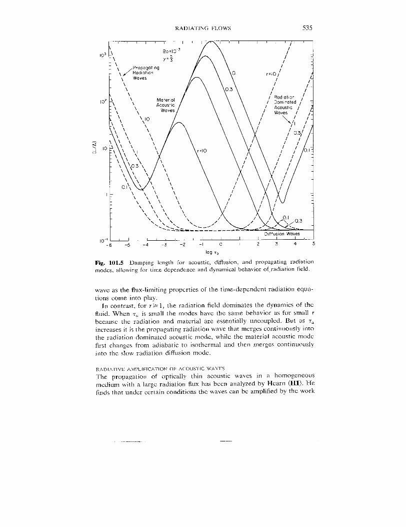
Fig. 101.5 Damping length for acoustic, diffusion, and propagating radiationmodes, allowing for time dependence and dynamical behavior of, radiation field.
wave as the flux-limiting properties of the time-dependent radiation equa-tions come into play.
In contrast, for r a 1, the radiation field dominates the dynamics of thefluid. When 7. is small the modes have the same behavior as for small rbecause the radiation and material are essentially uncoupled. But as ~.increases it is the propagating radiation wave that merges continuously intothe radiation-dominatecl acoustic mode, while the material acoustic modefirst changes from adiabatic to isothermal and then merges continuously
into the slow radiation diffusion mode.
RADIATJVE AMF’LI FICATION OF ACOUST(C WAVES
The propagation of optically thin acoustic waves in a homogeneous
medium with a large radiation flux has been analyzed by Hearn (HI). Hefinds that under certain conditions the waves can be amplified by the work
_——-

536 FOUNDAITONS OF RADIATION HYDRODYNAMICS
done by the radiation force on wave-induced variations of the opacity ofthe material. If the wave frequency is sufficiently low (but not so low thatthe disturbances become optically thick), radiative energy exchange oblit-erates temperature flactuations and the wave propagates isothermally. Inthis case the opacity varies only in response to changes in density, hence islargest when the material is compressed, which is also when it has the
greatest forward velocity. Thus the gas is most strongly accelerated when itis moving fastest in the same direction as the radiation flux, that is, whenthe radiation force is in phase with the velocity perturbation. Therefore thework done by radiation forces tends to increase the ve]ocit y amplitude of
the wave. On the other hand, high-frequency waves are essentially adiaba-tic, and the decrease in opacity with increasing temperature (which occursin hot, e.g., stellar, material) more than offsets the density-induced in-crease; hence these waves are damped by radiative energy losses. Unfortu-n ate] y man y approximations were made in this exploratory discussion, anda complete analysis using consistent Lagrangean radiation equations re-mains to be done.
An approximate theory describing the development of waves into thenonlinear regime under the action of this mechanism is contained in (H2).
102. Propagation of Acoustic-Gravity Waves in a Radiating Fluid
In this section we consider the propagation of acoustic-gravity waves in astratified radiating atmosphere. Unfortunately relatively little work hasbeen done on this important problem, and at present the state of theanalysis is far less complete and consistent than that presented in $101 forpure acoustic waves.
WAVEDAMP[NG BY NEWTONIANCOOLTWGConsider first the propagation of optically thin acoustic-gravity waves inwhich the radiative energy exchange produces Newtonian cooling. Weassume the radiation field is quasi-static, hence ignore its dynamicalbehavior. Under these assumptions the main effect of the radiation is todamp the waves. An additional effect, as we will see below, is that we nolonger obtain either pure progressive or pure standing (evanescent) waves
separated crisply into distinct regions in the diagnostic diagram as in theadiabatic case discussed in $53.
(a) [sotherrnal Atmosphere Following Souffrin (S16), (S17) we first as-sume a planar isothermal atmosphere composed of a perfect gas havingconstant specific heats. The linearized gas energy equation (10 1.3) thenreduces to
(dp,/dt] + w,(dpo/dZ) - a2[(dpJdt)+ w,(dpo/dz)] = –t~L[p, –(a2/y)p,].
(102.1)
RADIATING FLOWS 537
For simplicity we assume that the radiative relaxation time tRR is constant
with height. Assuming that p,, PL, and WI are of the form (53.30) we canreduce (1 02.1) to
i@P[l – (i/@tW)]– ia21wR[l – (i/y@tRR)]+ a2(@:/g) w = o> (102.2)
which differs from (53.3 Id) only by the imaginary terms in the coefficientsof itiP and ia20R. Here we used the fact that w; = (y – l)g/yFI for aperfect isothermal gas.
Although we can again use (53.30) for P, R, W, U, and 0, the verticalwavenumber k= will now be complex. For this reason we replace, for thetime being, ikzW and ikzP in (53.31a) and (53.31c) by –(dW/dz) and–(dP/dz), and combine those equations with (102.2) to obtain the follow-ing differential equation for W:
{(a2/a2) -[1 - (ti~/w2)]k~ - (1/4H’) + (d2/dz2)(102.3)
-(i/-y~t~~)[(yco2/a2)- k:- (1/4H2) +(d2/~z2)l}w= o
or
{hO+ (d2/dz2) - (i/-yatK~)[hO+ (d2/dz2) + (-y - l)(co2/a2) - (cd~/w2)k~]}W= O.
(102.4)
Identical equations hold for P or R. In the isothermal, adiabatic limithO= k: [see (54.89)].
Again following Souffrin we note that in general we can write kZ =
k~ + ik, and, assuming W K exp (–ik.z),
(d2W/dz2)--(h~ i- ih[) W= -(kK + ik1)2W= –[(kfi - k~)+2ik,kK]W.
(102.5)
Then substituting ‘(h* + ihI)W for (d2W/dz2) in (102.4) we find that h~
and h, are given by
where, as in 552, co. = a12H”. Tbe real and imaginary parts of k= aredetermined from hr = 2k~k[ and hR = k~– k?, which yield
k~ =~[h~ + (h:+ h?)’”] (1.02.8)
and
(102.9)
The positive sign was chosen for the radical to make both k~ and k:
positive (i e., k~ and k, real) whether h~ is positive or negative.
538 FOUNDATIONS OF RADIATION HYDRODYNAMICS
There remains an ambiguity about which sign of (k~)’/2 and (k;) ‘1’ tochoose. Souilrin imposes the requirement that the energy flux be positivein the positive z direction, that is, he requires that energy be carriedupward from a source. The vertical component of the energy flux is givenby
WW’cok. (w’- gzk;)(Ow)z = i(p”w+ Pw”) =
co4{k; +[k, – (1/2 H)+(gk;/ti2)]2}
(102.10)
which is positive if and only if
cok~(~4– g2k;)>0. (102.11)
If we multiply both sides of h,= 2kKkr by ~k~(~’– gzk~) and use (102.6)we find
k~k,o(~’– g’k;) =~hlco(a’– g’k;)(102.12)
= –[ytKR@2g2(l + 72w2t~K)](04- g’k;)’ <0,
which is negative because both factors in the right-most expression areintrinsically positive. Comparing (102.11) and (102.12) we conclude thatk, s O. Moreover we see that gravity waves, for which g’k~ > a4, havek~ <0 for upward propagation of energy, whereas acoustic waves, forwhich C04> g’k~, have positive k~, which was also the case for adiabaticacoustic-gravity waves as discussed in $54.
From (102.8) and (102.9) we see that when h~ = O, lk~l = Ikfl; whenhK>O, lk~l>lk[l; and when hl<<O, IkKl<lkrl. Thus when h~<O, thewaves are heavily damped over a single vertical wavelength, and were
classified by Souffrin as mainly damped or mainly evanescent, whereaswaves with h~ >0 are classified as rnuinly propagating. The boundaries
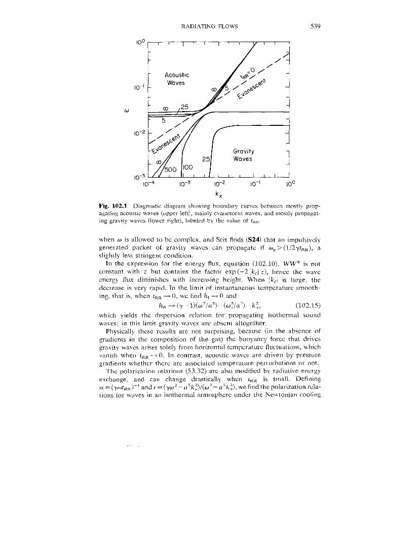
separating these propagating and evanescent regions in the diagnosticdiagram are defined by the curves h~ = O, and are shown in Figure 102.1for several values of tRR,ranging from O (isothermal) to cz (adiabatic).Damped, propagating acoustic waves lie above the upper curve, whichasymptotes at small values of k. to
@k(4uJ=W- (v&7) +{[@:- (Nwk)]z + (4@:/72&J}”2&(102.13)
which is the effective acoustic cutoff frequency in the Newtonian coolingapproximation. Note that O.N varies with tRR.The curve bounding theregion of propagating low-frequency waves asymptotes at large kX to
fiJ;N(tRR)= co- (1/y2t:R), (102.14)
the effective gravity-wave cutoff frequency in the Newtonian coolingapproximation. Thus if ti~ < (1/yt~~), gravity waves cannot propagate evenwhen the atmosphere is connectively stable. Equation (102.14) is modified
-. ---
100
,~-1
W
1(3-2
,0-3
RADIATING FLOWS
I I I I I I I I I Y I [ I
AcousticWaves
ml ,25
5/
k’/‘t-J’-dl(1111// /+~%
&.
Gravity
a) 25 Waves
500 100
,()-4 ,0-3 ,0-2 ,0-1 ,00
kx
Fig. 102.1 Diagnostic diagram showing boundary curves between mostly
539
prop-agating acoustic waves (upper left), mainly evanescent waves, and mostly propagat-ing gravity waves (lower right), labeled by the value of tRR.
when o is allowed to be complex, and Stix finds (S24) that an impulsivelygenerated packet of gravity waves can propagate if Ogs (1 /2yt~~), aslightly less stringent condition.
In the expression for the energy flLlx, equation (~ 02.10), WW* is notconstant with z but contains the factor exp (–2 Ikr] z), hence the waveenergy flux diminishes with increasing height. When Ikrl is large, the
decrease is very rapid. In the limit of instantaneous temperature smooth-ing, that is, when t~~ -+ O, we find hr -+ O and
h~ - (Y– l)(ti2/a2]– (@a2) – kf, (102.15)
which vields the dispersion relation for propagating isothermal sound,waves; in this limit gravity waves are absent altogether.
Physically these results are not surprising, because (in the absence ofgradients in the composition of the gas) the buoyancy force that drivesgravity waves arises solely from horizontal temperature fluctuations, whichvanish when tRR -0. In contrast, acoustic waves are driven by pressuregradients whether there are associated temperature perturbations or not.
The polarization relations (!53.32) are also modified by radiative energy
exchange, and can change drastically when t~R is small. Defining0! = (y@tRR) –‘ and r = (y@’– azk~)/(~2– a’k~), we find the polarization rela-tions fol- waves in an isothermal atmosphere under the Newtonian cooling
540 FOUNDATIONS OF RADIATION HYDRODYNAMICS
approximation are
(dLLql + h)
p = (ti2- a2k~)(l + r-2a2) {’.+”(’r-k)+’[(s)+ ’[-”’.l}~
cd(l+ira)
{R = (co’ -a’k~)(l + r2a2) ‘R
++[(;)(%)-:l+’(’-~ ”’.)}w
“+-iii)(102.16)
(102.17)
and, noting that (T1/TO) = (pl/pO) –(pi/pO) implies @ = (y P/az) –R,
@= 13(-y– 1)(1+ im)
(Q2- a’k~(l + r2a2) { ‘R+ ’’++[i-+(%)l}w ‘10218)The leading real and imaginary terms in (102.16) to (102.18) are the sameas in (53.32). The quantity r is of the order unity except when ti2 or -yti2 is
nearly equal to a2k~, while a can range from very small values (for nearlyadiabatic propagation) to very large values when 2mytRR is much less thana wave period.
(b) Solar Model Atmosphere In a nonisothermal atmosphere, use of theNewtonian cooling approximation provides a simple but, unfortunately,inconsistent method for studying the interaction between linear waves andthe radiation field. Some of the inconsistency arises from the fact that the
model atmospheres [e.g., HSRA (G3) or VAL (V4), (V5)] chosen torepresent the ambient medium in which the waves propagate are not inradiative equilibrium. Because the physical mechanisms that determine the
temperature structure of the solar atmosphere are not actually known, wehave little choice but to include an unspecified nonradiative source-sinkterm in the gas energy equation and write
Here F,,, represents some sort of nonradiative energy flux chosen such thatV - Fn, exactly balances the net radiative gains and losses in the staticatmosphere, that is,
[J.
4%- Ku(~u – S“) du 1o=(V oF,,,)O.o
(102.20)
Because we do not know how to write Fri., we cannot do more than guessat how a wave-induced perturbation (F.,), would depend on T] and p,.Therefore, in the linearized gas energy equation we have no choice but toignore this term altogether.
A second problem is that whenever the departure from radiative equilib-rium in the ambient atmosphere is large, the term f K,,,~(J,, – S.)O du, which

RADIATING FLOWS 541
is ignored in the Newtonian cooling approximation, can be large andimportant (cf. $100). Furthermore, in the Newtonian cooling formulation,the net radiative gain term 4rr ~ KVO(.~,,– SV)l dv is approximated in terms ofthe local cooling time, which is derived as if at each height the atmospherewere optically thin over a wavelength and infinite, isotropic, homogeneous,and isothermal at the local temperature. The cooling time is then calcu-lated from (1 00.17) and (100.10) using the local values of T(z), P(z), K(z),
etc. at each height; except in the low photospbere (KO/k) = O. However ascan be seen from Figure 54.1, each of the assumptions underlying (100.17)is poor in some region of the atmosphere, with the most serious errorsoccurring at continuum optical depths Tc - 10–2 to 1, where both T(z) andK(Z) vary rapidly with height, and where the gas is neither very opticallythick nor optically thin. Unfortunately this is also the region where theradiative damping effects are the most import ant.
Retracing the arguments of $100 it is clear that (100,17) is a poor
approximation to the solution of’ (1 00.7) for a highly inhomogeneous andan isotropic medium. Tn particular, in the solar photosphere and chromo-sphere the perturbations of J are essentially determined by the perturba-tions in S at an optical depth of abOUt unity, not locally. Hence thenonlocally driven part of J1 (which is lost in the local cooling-timeformulation) may dominate over the locally driven part.
In treating the propagation of linear acoustic-gravity waves in the solar
atmosphere we can take inlo account the variations of temperature,density, sound speed, buoyancy frecluency, and ionization properties of theatmosphere. The resulting varmtions with height of the real and imaginaryparts of the vertical “wavenumber” of a wave of given w and kX imply
height-dependent variations in all properties of the wave. To describeradiative-exchange effects the best treatments available all use the Newto-nian cooling approximation despite the criticisms we have just leveled at it;we merely caution the reader to remember the caveats expressed abovewhen evaluating the results of this work. Whether the results obtained areeven qualitatively correct can be determined ultimately only by computa-tions that treat the radiation field self-consistently with the fluid equations.
lf we assume the density to be fixed by the requirement of hydrostaticequilibrium, then, as in S54, the density is given by (54.75) with H(z)defined by (54.68). [See (M8) for a discussion about p(z), H, ti&, and uwhen a “turbulent pressure” is included in the model.] The amplitude
functions are again as in (54.77) with E(z) defined by (54.76), and theBrunt–Vaisiilii frequency co~v(z) is given by (54.67), ~o(z) by (54.69, and
r1{2jby (14.19).The linearized continuity and momentum equations are unchanged from
their adiabatic forms (54.78a) and (54.78b). The linearized energy equa-tion, written in terms of amplitude functions, becoines
i(d[~– (i/@tRR)]P(Z)– i@~2[l – (i/r@ tKR)]~(i)T (a2dV/g) ‘(z) = 0,
(102.21)

542 FOUNDATIONS OF RADIAHON HYDRODYNAMICS
orh(l- iary(2]- icoaz(l – i~)R(z)+(a20~V/g) w(z) =0; (102.22)
here CY= (r~t~~)-’ and 17= cP/cV including ionization effects as in (14.15)and (14.18). Combining (102.22) with (54.78a) and (54.78b) yields the
following rather unwieldy equation for P(z):
{($-l)k,+$-&+($)
[r(oz
– ia–-’:-*+($)+(+-+)($+31}’(Z)a=
‘{%F%%%) (102.23)
-+%J-(%$+%%%)(igr dlna+dlnr
)11P(z) = o.az dz dz
The expression in the first set of braces is identical to that in (102.3) except
that w~v and r replace w; and y, and a new term, which is identically zeroin an isothermal medium where H = HP, has appeared. The second set of
braces contains the derivative terms that arise because all the atmosphericproperties now vary with height. The terms containing derivatives of az,co~v, r, and (1/2H) are not exactly the same in the corresponding equa-tions for W(z) and R(z).
To obtain numerical results for a realistic model atmosphere it is easiernot to use (102.23) but to either (1) solve (102.22), (54.78a), and (54.78b)simultaneously at all depth points or (2) regard the atmosphere as a set ofthin layers, chosen such that no atmospheric property changes muchthrough a layer, and that the layer thickness is small compared to a verticalwavelength of the wave being studied. Within each layer all atmospheric
properties are taken to be constant, but the derivatives (dT/dz) and (dw/dz)obtained from the model are used to calculate H and O;v (which in turnare taken to be constant within a layer).
We will describe results obtained by using method (2). All terms in thefirst set of braces in (102.23) were calculated as they would be for a
continuous model; the value for each layer was then chosen to be eitherthe midpoint of the layer or at an interface. All terms in the second setof braces were assumed to be negligible and were dropped. Becausethe approximations inherent in the original equations imply that at bestonly qualitative results will be obtained, the small inaccuracies incurred inthis implementation of the 1ayer method are not important.
We will discuss only gravity waves, t’or which the region of propagationlies above about 100 km, where t~~ > l/rco,zv [cf. (102.14)]. The adopted
radiative relaxation times are given by the linear relation shown in Figure102.2, which closely approximates the relaxation times computed by Stix
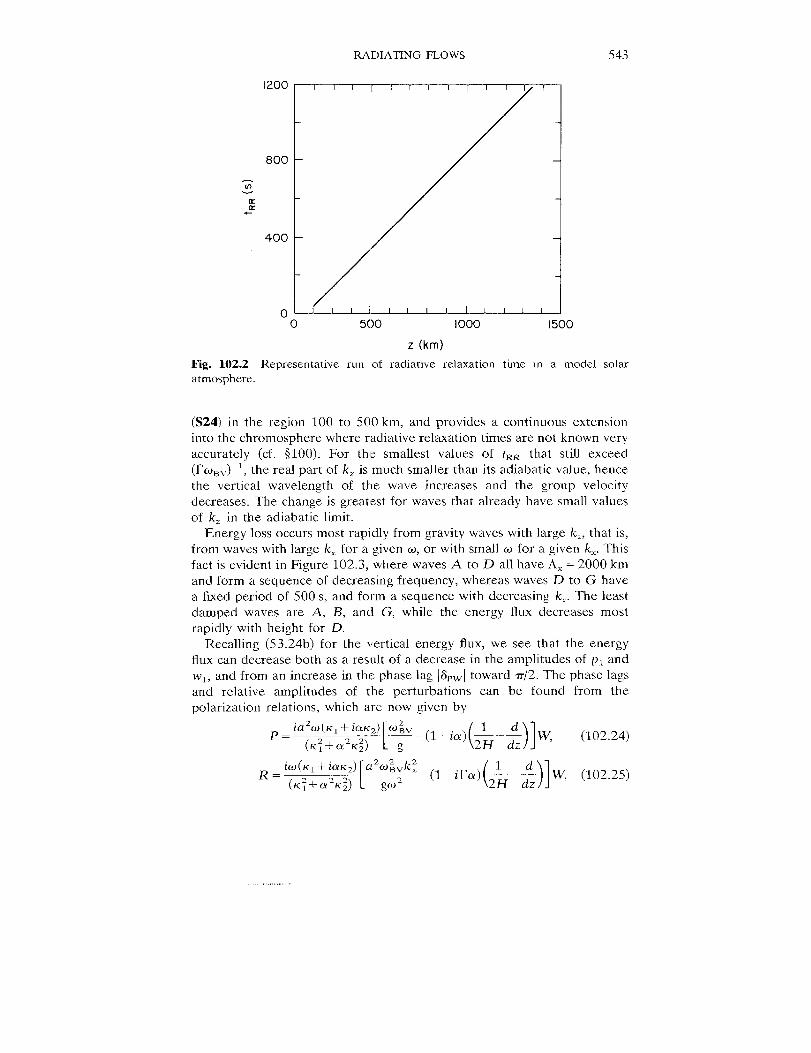
1200
800
-ZaK
400
RADIATING FLOWS
I I i I I [ I I I I I I I
/
543
“o 500 1000
z (km)
Fig. 102.2 Representative run of radiative relaxationatmosphere.
(S24) in the region 100 to 500 km, and provides a
1500
time in a mode~ solar
continuous extensioninto the chromosphere where radiative relaxation times are not known veryaccurate] y (cf. $100). For the smallest values of tRR that still exceed(ro~v)-l, the real part of k= is much smaller than its adiabatic value, hencethe vertical wavelength of the wave increases and the group velocitydecreases. The change is greatest for waves that already have small valuesof k= in the adiabatic limit.
Energy loss occurs most rapidly from gravity waves with large k=, that is,
from waves with large k. for a given ~, or with small ~ for a given k.. Thisfact is evident in Figure 102.3, where waves A to D all have A. = 2000 kmand form a sequence of decreasing frequency, whereas waves D to G havea fixed period of 500s, and form a sequence with decreasing k.. The leastdamped waves are A, B, and G, while the energy flux decreases mostrapidly with height for D.
Recalling (53.24b) for the vertical energy flux, we see that the energyflux can decrease both as a result of a decrease in the amplitudes of p, and
w,, and from an increase in the phase lag 18Pwl toward m-/2. The phase lagsand relative amplitudes of the perturbations can be found from thepolarization relations, which are now given by
P=[–-(l-iakkalw ‘10224)
k12C0(K1+ ~CLKZ) @~v
(K~+CK2K~)– g
R=[
‘@(K’+ ‘a”) a2:~k:-(1- iIh)(&-:)] W, (102.25)(K~+CY2Kj]
. ... .
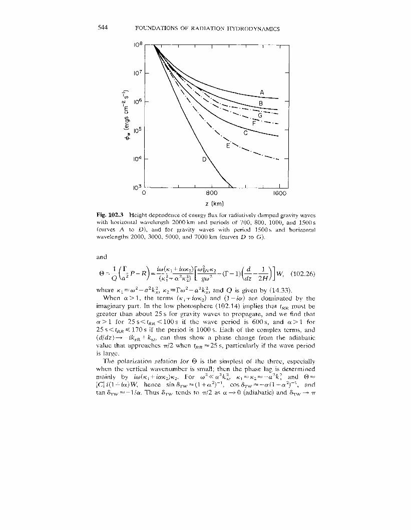
544 FOUNDATIONS OF RADIATION HYDRODYNAMICS
108 I
107 –
-in
y ,06 .
EvmCn
& ,05 _
-&
104 – D
,03. I 1 I I I Io 800 1600
z (km)
Fig. 102.3 Height dependence of energy fltlx for radiatively damped gravity waveswith horizontal wavelength 2000 km and periods of 700, 800, 1000, and 1500 s
(curves A to D), and for gravity waves with period 1500 s and horizontalwavelengths 2000, 3000, 5000, and 7000 km (curves II to G).
an cl
@=;(%~)= (.,+.2.;, [~+d-alw ‘10226)i@(K1 + iCtK,) @:vK~
where Kl=w2—a2k~, K2~~~2 – azk~, and Q is given by (14.33).When a > ~, the terms (Kl + iCIK~) and (1 – ia) are dominated by the
imaginary part. In the low photosphere (102.14) implies that t~~ must begreater than about 25 s for gravity waves to propagate, and we find thata >1 for 25 s< tRR<100 s if the wave period is 600 s, and a >1 for25 s < tRRs 170s if the period is 1000 s. Each of the complex terms, and
(d/dz) ~ –ikz~ + k=,, can thus show a phase change frolm the adiabaticvalue that approaches 7r/2 when t~~ S=25 s, particularly if the wave periodis large.
The polarization relation for @ is the simplest of the three, especiallywhen the vertical waven umber is small; then the phase lag is cfetermi nedmainly by ~OJ(Kl+hK2)K2. For @z<< azk~, K, =K2=—a2k~ and @=ICI i(l +ia)W, hence sin 8-rw=(l+a2)-’, cos 8-rw=–ci(l+ct2)-1, andtan ?l-rw= –l/a. Thus S~w tends to rr/2 as a -0 (adiabatic) and i3.W ~ T
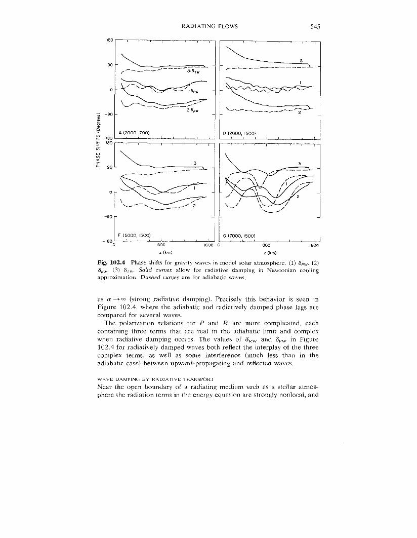
RADIATING FLOWS 545
90 –
o –
-./ _— -- -— -- 3:s~w
es._—--2:8PW
\ I
i,,o~0 800 1600
z (km)
1 ( , I , , , I
~F—-.——.—- -— —___
D (2000, 1500), I I I , I 1
r 1 1
3——. .
/ /
*
/—,- J
\//
,/ ‘ ,/
// \\
2
\d/ \\ L ,/
G (7000. 1500)1 ! , I ) 1 , I
800 16CKI
z (km)
Fig. 102.4 Phase shifts for gravity waves in model solar atmosphere. (1) &w. (2)
i5Pw. (3] 8-. SoLid curves allow for radiative damping in Newtonian cooling
approximation. Dashed cuwes are for adiabatic waves.
as a -+ VJ (strong radiative damping). Precisely this behavior is seen inFigure 102.4, where the adiabatic and radiatively damped phase lags arecompared for several waves.
The polarization relations for P and R are more complicated, eachcontaining three terms that alre real in the adiabatic limit and complexwhen radiative damping occurs. The values of 8RW and 8PW in Figure102.4 for radiatively damped waves both reflect the interplay of the threecomplex terms, as well as some interference (much less than in theadiabatic case) between upward-propagating and reflected waves.
W+\VE DAMP [NG BY RAOl ArIVE “IWANSPORT
Near the open boundary of a radiating medium such as a stellar atmos-phere the radiation terms in the energy equation are strong] y nonlocal, and
546 FOUNDATIONS OF RADIAHON HYDRODYNAMICS
should be determined from the transfer equation. To study the radiativedamping of acoustic-gravity waves in a realistic model solar atmosphere,Schmieder (S5), (S6) coupled the linearized fluid equations to a linearizedtransfer equation. Because the perturbation J,,, of the radiation field ateach depth then depends on T, at all depths, the fluid equations at onedepth become globally coupled to those at all other depths.
Several approximations were made to simplify the equations. First, thewaves were assumed to propagate in the vertical direction only, hencek.= O and the problem becomes strictly one dimensional. Second, LTEwas assumed, so all material properties can be written as functions of p andT. Third, the perfect gas law was used and ionization effecls are neglected.Fourth, the radiation field was assumed to be quasi-static, hence itsdynamical behavior was ignored. Schmieder analyzed waves in the regionfrom an optical depth of about 3 up to a height of 500 km, that is, the top
of the photosphere. The assumption of linearity gradually breaks downwith increasing height, but should be quite good in the lower layers whereradiative damping is most important.
The run of temperature and density was taken from the HSRA model
solar atmosphere (G3]. The ambient atmosphere is thus neither in radia-tion nor in hydrostatic equilibrium. The linearized continuity and momen-tum equations are given by (52.24) and (52.25) (ignoring the non-gravitational force term that is implicit in the HSRA model). These can berewritten in terms of the vertical displacement <1, defined by WI = (d<l /dt).Thus integrating (52,24) over time we have
(3L+ <l(dpo/dz)+ po(d<, /dz) = o, (102.27)
while (52.25) becomes
Po(~2L1/dt2) = –(alp ,/dz) – p, g. (102.28)
The gas-energy equation (ignoring the nonradiative term that drives the
ambient atmosphere out of radiative equilibrium) becomes
PO dTI \ M, dTo _(Y-l)Po~ dL,
(poTO dt at dz–-) Pa (-)dz at(102.29)
=47r(7-1)[~m
Kuo@v I ‘-TU1) d~+
r 1KVI(~,,O— ~,>0) d~ .
0 0
The first term on the right-hand side results from the wave-induced
perturbations of the mean intensity and the local Planck function. Thesecond term arises from two effects: (1) the perturbation of the opacity,and (2) the departure of the ambient atmosphere from radiative equilib-rium, which i]mplies that JO # Elo. When .fO– 130 is large, the second term,which is strongly model dependent, may also be large; thus errors in theassumed T(z) of the unperturbed model may produce important errors inthe radiative damping calculations.
RADIATING FLOWS 547
The mean intensity is approximated by the average of the incoming andoutgoing intensity calculated frc)m the formal solution (79.14) and (79.15)for a representative ray, using the Planck function from the model atmos-phere. The radiative energy exchange term in (102.29) is approximated bya quadrature sum over a few representative frequencies. Perturbed inten-sities are computed from the linearized formal solution, which is con-
structed recursive y between successive depth points in a discrete mesh. Topose boundary conditions for the transfer equation, it is assumed that thereis no incoming radiation at the top of the atmosphere, whereas the bottomof the atmosphere is taken deep enough that the diffusion approximationcan be applied. The hydrodynamic boundary conditions are imposed at theupper boundary where the value of <1 is fixed; all perturbations arcnormalized to this value. Initial relations between T~ and ~1 at theuppermost two grid points are obtained by assuming adiabatic motion anda pure outgoing wave at the top of the atmosphere. The resulting matrixequation is solved numerically and iterated to consistency.
In Schmieder’s solution the general form of the radiative exchange terlmat depth point i is
@i = ~ AiiTl,j + z Bii~[,i. (102.30)j ;
The matrix Bii is almost diagonal. The matrix Aii, however, clear] y revealsthe strong non local effect of the radiation-field perturbations produced bytemperature perturbations up to about one photon mean free path awayfrom the chosen depth i. For heights above about 200 km the dominantcontributions to qi from Aii come from (1) a region between about –40 kmand +140 km, and (2) the local temperature perturbation, which prOdUCeSthe diagonal elements. The departure of the ambient ~...] osphere fromradiative equilibrium also makes an important contribution to the diagonalelements. Below 200 km, the opacity increases exponentially, and thelargest off-diagonal elements in Aii become confined to a small range of
depths immediately above and below the point Zi. At large optical depths,a photon mean free path becomes small compared to the grid spacing and
Aii becomes essentially diagonal.Schmieder finds that the wave amplitudes increase less rapidly with
height for radiatively damped waves than for adiabatic waves. Evanescentwaves are less affected by radiative damping than propagating waves;therefore akhOUgh the amplitude of an adiabatic evanescent wave growsmore slowly with height than that of a propagating wave, the difference ingrowth rates between radiatively damped evanescent and propagatingwaves is not large. For example, for a 140-s propagating nonacliabaticwave, the relative temperature perturbation (lrrll/To ]w, 1) is distinctly sup-
pressed compared to that of an adiabatic wave in the region of strongclamping. For a 300s evanescent wave, however, the relative temperatureperturbation is actually larger in the nonadiabatic case than in the adiabaticcase.
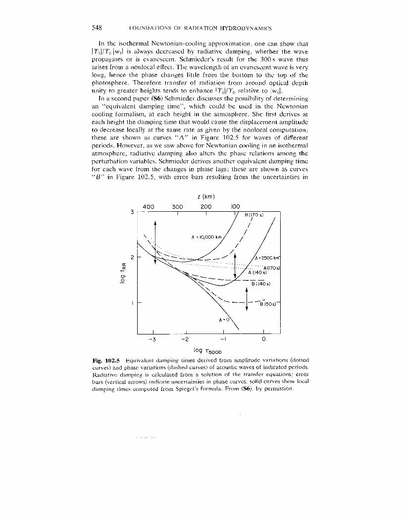
548 FOUNDATIONS OF RADIATION HYDRODYNAMICS
In the isothermal Newtonian-cooling approximation, one can show thatIT1l/’TOIWll is always decreased by radiative damping, whether the wavepropagates or is evanescent. Schmieder’s result for the 300s wave thusarises from a nonlocal effect. The wavelength of an evanescent wave is verylong, hence the phase changes little from the bottom to the top of thephotosphere. Therefore transfer of radiation from around optical depthunity to greater heights tends to enhance IT1l/TO relative to Iw ,1.
[n a second paper (S6) Schmieder discusses the possibility of determiningan “equivalent damping time”, which could be used in the Newtoniancooling formalism, at each height in the atmosphere. She first derives ateach height the damping time that would cause the displacement amplitudeto decrease locally at the same rate as given by the nonlocal computation;these are shown as curves “A” in Figure 102.5 for waves ot’ different
periods. However, as we saw above for Newtonian cooling in an isothermalatmosphere, radiative damping also alters the phase relations among theperturbation variables. Schmieder derives another equivalent damping timefor each wave from the changes in phase lags; these are shown as curves“B” in Figure 102.5, with error bars resulting from the uncertainties in
z (km)
400 300 200 1003
2mLY
cmo—
I
I I I I
A
\ A = 10,000 km,.,
,\
~.o
I I I
–3 -2 –1 o
109 75000
Fig. 102.5 Equivalent damping times derived from amplitude variations (dottedcurves) and phase variations (dash ed curves) of acoustic waves of indicated periods.Radiative damping is calculated from a solution of the transfer equations; errorbars (vertical arrows) indicate uncertainties in phase curves. solid curves show localdamping times computed from Spiegel’s formula. From (S6), by permission.

RADIATING FLOWS 549
assigning phases in waves that vary strongly with height. The two sets ofcurves give markedly different results. Had damping times been estimatedfrom amplitude ratios, yet different results would have been obtained.
For comparison, damping times computed for waves of the satne periodsusing Spiegel’s formula (100.17) are shown in Figure 102.5 as solid curves.The important conclusion to be drawn is that nonlocal effects resultingfrom radiative transfer produce qualitatively different propagation charac-teristics in a wave, and that it simply is not possible to reproduce theseeffects self-consistently with a single equivalent damping time.
STABILITYOF .4COUSTr C-GRAVITY WAVES IN A RADIATING FLUID
The possibility of radiation-driven instabilities in a stratified radiatingatmosphere has been discussed by Berthomieu et al. (B4) and by Spiegel(S19). In the former paper, it is shown that above a certain criticalfrequency, isothermal, optically thin pert urbations in an isothermal slab ofan atmosphere traversed by a radiation field can be amplified by radiationin a drift instability. In the latter paper it is shown that under certain
circumstances radiation forces can drive instabilities in a stratified radiatingfluid. A detailed analysis is presented for quasi-adiabatic photoacoustic andphotogravity modes. The results are intriguing, but it would take us too farafield to discuss them here; the interested reader should consult theoriginal paper.
8.2 Nonlinear Flows
103. Thermal Waves
Thermal waves result from conductive energy-transport processes within afluid, which give rise to an energy flux q = –K VT. For nonradiating neutralgases it is usually satisfactory to assun~e linear conduction (K independent
of T) because the conductivity depends only weakly on temperature (cf.$33). But in ionized plasmas where K x T5’2, and in opaque radiating fluids
where the radiation conduction coefficient depends strongly on T, we musttreat nonlinear conduction. The distinction is important because thermalwaves behave qualitatively differently in the two cases.
A prob~em of some interest in radiation hydrodynamics is the penetra-tion of radiation from a hot source into cold material, a process that isreasonably well described by treating the radiation field in the diffusionapproximation. Practical examples are the penetration of stellar radiationinto the interstellar medium at the instant of star formation or of asupernova explosion, or the irradiation of a fusion pellet by intense laserbeams. Such propagating radiation fronts are called Marshak waves (M4)
or radiation difhmion waves.Because radiative energy exchange is very efficient, significant radiation
penetration and energy deposition can occur in a time much too short for