DENSE AND NON-DENSE FAMILIES OF COMPLEXITY CLASSES

*Borodin, A. , Constable, R.L., Hopcroft, J.E.

Cornell UniversityIthaca, New York

* University of Toronto

Abstract

Let t be any abstract measure ofcomputational complexity, and let L de­note the specific measure of memoryresource (tape) on one tape Turing machines.

De~ote by R:( ) the class of all totalfunctions whose t-complexity is bounded bythe function t( ) almost everywhere. Callsuch classes t-complexity classes. Weare interested in relationships amongthese classes, under proper set inclusion(C). In other words, we are interestedin the partially ordered structure

<I·,.~ where I· = {R:( ) It( ) is re­cursive} is called the family of t-com­plexity classes. Of special interest is

the subfamily O· {R:. ( ) Iti ( ) is1

total} , called the family of e'xact.~complexity classes.

We show that EL and OL are denseunder C for sufficiently large bounds t( ),

. Lbut nL is not dense in L • We also con-

struct measures ~ for which L~ and ot

are non-dense, for which L~ is dense but

Qt is not, for which O~ is dense but Lt

· ~. d · ~tis not and for wh1ch.0 1S ense 1n ~

Thus density is not a measure invariant~~.... t ~property of L or 0 • These are thefirst examples of important structuralproperties of these families which are notmeasure invariant.

I. Preliminaries

We assume at least cursory famil­iarity with the axiomatic approach tocomputational complexity theory as in­itiated in Blum [1] and developed recentlyin [2], [6], and [9]. To establish ournotation, we list the following defini­"·tions.

Given an acceptable indexing {~i( )}

~f the partial recursive functions (of oneargument), see Rogers [8], an abs~ract

complexity measure over {~i()} 1S a set(t. ( )} of partial recursive functions for

1~hich there exists a 0,1 valued recursive

7

function M( ) satisfying

Axiom 1: ~i(n) is defined iff ti(n) isdefined.

Axiom 2: M(i,n,m) 1 iff ti(n) = m.

We say that ~ {ti ()} satisfying

the axioms is a complexity measure, and theindividual t. () are called exact com-

1plexity functions. [The t i () have also

been called "step-counting" functions or"run-time'" mnctions or "difficulty"functions.]

Given a complexity measure t , define

a t-complexity class R: ()= {~'i ( ) 1

~. ( ) total and t. (n) < ten) for almost all1 1 -

n (a.e.n.)}. (We use lower case Englishletters, t,f,g,h, in denoting total asopposed to partial functions.) When t isclear from the context we use Rt ( ) •

Define r t = {R:()I t( ) is recur­

sive} and ot = {R:.o() I t i total}

1

Call L~ the family of (recursive) complex-

ity classes and ot the famil¥ of exactcomplexity classes (or run-t1me c~s).Our concern is with the families L~ and

ot under the partial ordering of setinclusion, c. A set S partially orderedby < is dense iff for all a,b in S,a <-b i~plies there is a c in S suchthat a < c < b •

We say that any family C~ of complex­ity classes is dense for sufficiently large!i-L iff there is a function a() such

that the family {R:() I t( » a( ) &

t( ) recursive} n c t is dense (under c ).

II. Density

Our Turing machine model is that usedin Hartmanis & Stearns [3]. It uses separ­ate input, output and work tapes and usesthe standard finite control over a finitealphabet E • We consider the class of allsuch machines over all finite alphabets LLet {M.} be an acceptable listing of such

1

machines and <Pi () the one argument

function computed by Mi. Define the

tape measure L as follows: L = {L. ( )}J.

where

L. (n) =+

the maximum number oftape squares used inthe computation of Mion input n (inbinary)

undefined

if thecomputation

halts

otherwise

sequence {n~} such that Li ( is non­

decreasing 9n {n1 } , i.e.,

Li (n1 ) ~ L(n1+1) and

Li (n 1) < Lj (n1 ) for all 1

We construct a suitable Mk by guar­

anteeing that we alternate between Li ()

and L.() on an infinite sequence as]

above. The amount of tape used by Mk on

input x is determined as follows:

It is easy to see that L is indeeda complexity measure.

Def. 2.1

Layoff Li(X) tape (run Mi , put

down markers to indicate boundaries of thetape used and then erase all other markson the tape).

Q.E.D.

xDiagram

L. (x) < L. (x) , then constructJ. J

unique finite sequence'{ml , m2 ,

••• mr } where

~rn {Li(m) < Li(X) & Li(m) <

Lj

(rn) }

~m {m > mp & Li(m) ~ Li(X) &

Li(m) < Lj(m) & Li(mp ) ~

Li(m)}

~+l

the

(1) If L. (x) < L. (x) , then make] - J.

Lk(X) = Li(X). (There are possibly

finitely many x s~ch that Lj(X) <L

i(x) .)

(2) -If

* denotes Lj(Y) where Lj(y) > Li(y)

If r is odd, then set Lk(X) = Li(X).

If r is even, then set Lk(X) = Lj(X),

The Mk and Lk ( ) produced by the con-

struction will satisfy the theorem sinceLk ( ) will alternate between Li ( ) and

L. ( ) on the infinite sequence of pointsJ

{ml , m2 , ••• }

Given machines M. and M. with tapeJ. J

comp~exities Li () <. Lj ( we

show how to construct a machine Mksuch that Lk ( ) satisfies the

theorem, i. e., Li ( ) <. Lk ( ) <:. Lj ( ).

If L. ( ) were non-decreasing, thenJ.

the proof would be trivial, namely todefine Mk on input x; run 'i(y) , mark

the amount of tape used, then run ~. (y)J

until it stops or attempts to exceedL. (y) tape. Record which was greater, i

J.or j. Do this for all y ~ x and deter-mine for how many y, Li(y) < Lj(y).

(It is essential to note that this can bedone for each y without exceeding Li(y)

(the lower bound) amount of tape.) Ifthe number of such y is even, thenstop Mk having used Li(X) tape; if odd,

then let Mk run and use Lj(X) tape.

Thus infinitely often Lk () will be above

L. ( ) and infinitely often L. ( ) will beJ. J

above Lk (). Thus Li () <. Lk ( ) <.

L. ( ) •J

f ( ) <., g ( ) iff f (x) < g (x) a. e. xand -

f(x) < g(x) i.o. (infinitely often)

However, Lit) need not be non­

decreasing. But L. ( ) <- L. ( ) doesJ. J

imply that there exists an infinite

The tape complexity functions aredense under <••

Proof

Theorem 2.1 (Borodin, Hopcroft)

8

Lemma 2.1 inf Li(n) = 0 andn-+oo

Lk(n)L L-:j <P iffRL. ( Rt (

1. inf Lk(n) 0inf ten) 0 . n-+oo L:l'iifn+oo L:lIir

1. J

Proof

Q.E.D.

Proof-

Moreover, by Lemma 1. 1, RL . ( ) c ~ . ( )1. J

The value of this constant is de­termined by knowing the history of Li (

and Lk () on Sx ' that is, by knowing

the largest constant for which 2(b) hasalready been satisfied. Step (2) guaran­tees that for each c an appropriate

(3) We describe the operation of Mkon input x. The definition of Lk(X)

requires the reconstruction of Lk () on

a finite sequence Sx = {nl , n 2 , ••• , nr }

wheren l = ~n[Li(n) ~ Li(x)]

np+l ~n > np[Li(n) ~ Li(X)]

and nr = x

First Mk lays off Li(X) tape.

Using a multi-tract tape, ~ finds out

which points z ~ yare not in Sx' and

marks them on one track (put a - on theappropriate track in the cell correspond­ing to z). This merely requires tryingto compute <Pi(O), <Pi(l), •.• , <Pi (x) •

Now for each yeSx ' reconstruct the com­

putation Mk on y to determine the value

of Lk(y). Also attempt to satisfy 2(b)

for the largest possible c.

inf Li(X) 0, there is at least onen+oo L:lXr

J

infinite sequence S = {ml , m2 , m3

, ••• }

such that(a) for all ~, Li(m~) < Li(m~+l)

(b) for all c there is an mes andyeS such that ceLl (m) < L. (m) <L. (y) • 1. J

1.

To this end, we construct Mk so that

Vc :iI x :iI x such that c·L. (x ) <c l c 2 1. Cl

L. (x ) and Lk(Xc ) Li(X ), c·L. (x )<J c 2 1 c l 1. c 2

Lj(Xc ) and Lk(Xc ) L . (x ).2 2 J c 2

(2) Since Li(X) ~ 2x and

.)

Li(n) = O.L. (n)

J

infn+oo

Without loss of generality we assumeL. (x) < L. (x) for all x • (RL . ( ). C

1. J 1.

implies :ic L. (x) < c·L. (x)1. - J

Replace Lj () by

implies

~j(for all x •(c + 1) eL. (

J

that

(1) "only if case" If inf t ( ) :j 0,n-+oo Li(n)

then :iI c such that t (n) ~ c eLi (n)

a.e.n. Since L has a linear globalspeed-up, ~. ( ) ,= Rt ( ) •

1.

(2) "if .case" We need to "reprove"the well-known results of [4] sinceour tape measure has been defined asa function of the actual inputrather than of input length. Weleave this proof for the interestedreader.

In order to simplify the proof some­

what we will assume that L. (x) > 2x for1.

all x (a.e. x). We note, however, thatit would be sufficient to require onlyl~m inf Li(n) + 00.

n-+-oo

Theorem 2.2 (Borodin, Hopcroft)

nL is dense for sufficiently larget( ), i.e., for all sufficiently largeLi ( ) such that RL . ( ). c ~. ( ) ,

1. Jthere is an Lk () such that RL . ( ) ,c

1.

R-. C R-~k ( ). L j (

(1) We will construct a machine Mk.0 that Lk ( ) oscillates between Li ()

~d Lj <) and Lk ( ) satisfies

9

-{

- i - i j -

Proof

L. (x) < L.. (x)1. - -k

so that

infS

at least one

Clearly

is dense for sufficiently large

< L. (x) • Thus,- J

RL ~ rLi

( ). C --r;k ( ). C -L.j

( ) •

Q.E.D.

Moreover, for all x,

The computation of Mk on input x

uses Li(X) tape up to the time when

we decide whether Lk(X) = Li(X)

or Lk(X) = Lj(X).

Lk ( ) oscillates on

infinite sequence S

inf Li () = 0 and

S r:;r>

desired function.

A somewhat more intricate version ofthe previous (run-time density) proof isneeded. The difficulty is that we are nolonger assuming that t l () and t 2 ()

are tape complexity functions, only thatthey are recursive functions. That is, weassume for sufficiently large t l (), t 2 ( )

that Rt1

( ).c Rt2

( ) , and we seek a

t 3 ( such that

* Rt1 ( ). C Rt3 ( ). C Rt2 ( )

(1) We first notice that we can re­place t l () by another recursive func-

tion ~() such that Rt () = Rt ( ) and- 1

~( ) ~ t 2 ( ) a.e. To see this, suppose

t l ( ) > t 2 () i.o. Then put S ='{xl

tl(x) > t 2 (x)}. We claim that

tl(x) if xtslex) = t (x) if XES is the

2

(B)

Theorem 2.3 (Borodin, Hopcroft)

(e)

The reader is asked to verify thefollowing:

(A) For all x the Lk () history track

represents exactly the value ofLk(y) for all YESx •

L. work trackJ

L. work trackl.

Lk history track

constant counter trackLi(X) squares long

where .i,in square y of Lk ( ) history

im~lies YESX

and Lk(y) = Li(y)

j in square Y of L k ( ) history

implies YESx and Lk(y) = Lj(y)

- in square Y of L k ( ) history

implies ytsx

I in square Z of Lk ( ) history

while reconstructing Lk(y)

implies that Mk will attempt

to determine if ceLl (z) < L. (z)J. J

using ~ Li(y) tape.

(4) We give a brief informaldescription of ~. Our proof depends on

our ability to make Lk () oscillate on

the sequence S = {ml , m2 , ••• } so that

inf Li(n) = 0 and inf Lk(n) = 0 •n-+-oo~ n-+oo~

Lk\n) Lj(n/

Suppose that using our alternating valuescheme we have set Lk(mp ) = Li(rop) and

the maximum constant is c. The idea isto then define Lk(IDp+I) = Li(IDp+l)'

Lk (IDp+2) = Li (mp +2) , ••• until we can

detech (at some y = ms ) that for some z

in S, C.Li{Z) < Lj(Z) and Lk(Z) was set

to Li(Z).

We then begin to define Lk(ms ) =Lj{ms )' Lk(ms +l ) = tj(ms +l )' ••• until

we detect (at some later y' = rot) that

for some z', c'L. (z') < L.(z') and1. J

Lk(Z') was set to Lj(Z') • At this

point the value of the constant increasesto c+1.

x and x will come up. Now use anc l c 2alternating values scheme to determineLk () just as done in Theorem 1.

During the computation, the worktape of Mk could appear as follows:

10

(3) We construct Lk () at a point

x by reconstructing (as before) asmuch of the past history of Lk () as we·

can in L. (x) tape. The only modifica-~ .'

Suppose only R c R Then theret ( ) - t l ( ).

is an Li ( such that inf t 2 ( ) = 0 byS L:T>

~

Lemma 2.1 and Li ( ) ~ t 1 ( ) a.e. Thus

~i ( ),~ Rt1 () and ~i ( ). c Rt2 ( ) .

The proof requires a more elaborateversion of the construction of Mk , but

the general ideas are the same.

Q.E.D.

Corollary 2.1 (Borodin)

Between any two sufficiently largecomplexity classes there are an infinitenumber of incomparable complexity classes.

We leave to the reader veriffcationthat a machine ~ can be defined such that

(A) for all x Lk(X) Li(X) or

L k (x) = L j (x) •

(B) for all c there exists xc'1

x such that c-t(x ) <c 2 - c 1L. (x ) and Lk(X ) = Li(X ),] ,c

lc

lc

lc-t(x ) < L.(x ) and- c 2 ] c 2L

k(x ) = L. (x ) •c 2 ] c 2

By making some assumptions on thegrowth of Li we can guarantee that for

all z there is an x such thatLi(X) > tnax{Lt(z), c-!:.(z)} where~t ~ t.

Thus the construction of Mk is very

similar to the construction for run-timedensity. The reader can easily verifythat condition ** of (2) is satisfied.

tion is that we do this reconstructionrelative to t() (more precisely, rela­tive to a fixed algorithm ~t for t()

with tape complexity Lt () ).

That is, while computing thie historyof L. ( ), Lk ( ), and L. ( ) we also com-

~ ]pute the history of !( ) on those values

for which the computation is possiblewithin Li(X) tape. We then determine

whether L k () has been set equal to

L. ( ) for an even or odd number of times]

on a set of points for which L. (y) >]

c-t(y) for larger and larger c. The moredifficult t() is to compute, the moreancient is the history which determineshow we set the value of Lk(X) . By

picking a sequence of points P on whichL i ( ) grows monotonically we can use the

history to guarantee oscillation on a setof points S for which lim t() o.

S ~. ( )1.

We

ando

Diagram

L j ~

** Rt ( ).c !\nax{!( ),Lk

()} C

R C R-1nax{! ( ), L j ( )} . t 2 (

We accomplish this by making Lk (

oscillate between Li () and Lj ( ), but

we must ensure that this oscillationtakes place on an infinite set of pointsS such that lim t() o. The desired

S ~. ( )]

effect will be that

Let Lj(X) = max {Li(X) + 1, Le(X)}

shall attempt to construct Lk <') such

that

But this contradicts Rtl ( ) ~ c Rt2 ( ) •

(2) We now proceed to find a recur­sive t 3 () satisfying * Let i be

such that Li ( ~!() a.e. Since

R!( ):c Rt2

( ) , there is an e such

that Le () < t 2 ( ) a.e. and

inf !(n) = 0 •n+oo :r-r=)Le\n

11

III. Measures for which

E~ and n~ are non-dense.

In order to construct our example of

a measure ~ for which E~ and n~ are non­dense we need three basic facts. Theseare given below.

We need one more basic fact beforeconstructing our non-dense measure. Thefact is simply that for every measurethere is a uniform bound on the value ofthe function given its complexity. Forexample, if Li(x) = y, then for a binary

machine ~. ( ) < 2Yl. -

(Compression)Theorem 3.1 (Blum)

(Bounding)Lemma 3.1 (McCreight & Meyer)

The proof is elementary. Blum [1]has proved that any two measures ~ andA

~ are related by an A increasing d'()

such that ~i(n) < d(~i(n),n) andA

~i(n) < d(~i(n),n) a.e.n.

Proof

For all ~ there is an increasing g()such that for all i and for all suffi­ciently large ~i( ), ~i(n) < g(~i(n» a.e.n.

( Gip)Theorem 3.2 (Borodin)

For all ~ there is a partial re­cursive p() such that for all recursive~e( ) and for all ~i( )

To use this fact here we observe that(a) ~p(i,e) (n) is defined iff ~i(n) for the tape measure L = {Li ()} the

is defined lemma surely holds, say for gL( ) • Thus(b) if ~i(n) is defined, then picking a d() relating ~ and Lm , it

$i(n) < $p(i,e) (n) follows that $i(n) < gL(L~(n) ) <(c) for all i there is no ~. (

J gL(d(~i(n),n) a.e.n. Now take g(n) =such that for infinitely many " 0 0

n ~. (n) is defined and gL (d (n) ,n) , and suffl.cl.ently large"p(l.,e)

~ 0 (n) < ~ 0 (n) < cJ> (~o (n) ) •means for all ~i ( ) such that ~ 0 (n) > np(l.,e) - J - ·.e p(l.,e) l. -

a.e.n.

For all ~ there exists an h(),called. a jump function for ~ (sometimesdenoted h~( ) ) such that for all

sufficiently large ~. ( )1.R~. ( ). C Rh ( ~. ( » •

l. l.This is proved as Theorem 8 of Blum [1] •

That is, ~p(i,e) ( ) is a "~e( ) gap above

~ i ( ).n

Q.E.D.

Theorem 3.3 (Constable)

Proof

There exists a measure ~ such thatA A

there are arbitrarily large ~o ( ), ~o (satisfying 1.1 l.2

(i) R~ 0 ( ). c R~ 0 () andl.l l.2

(ii) there is no recursive t()such that\ R;o ( )~c Rt ( ).c

1.1

Our method of proof is quite trans­parent. We select an appropriate gap sizeh( ) = ~e() and use the technique of

Borodin's Gap Theorem to find for each~o () a gap function ~ (0 ) ( ) above1. p l.,e

R~ 0 ( ) •

l.2

That is,' neither E~ nor n~ is dense.(2) Define ~ (0 len) = lJY[Y>~o(n)p l.,e l.and P(y,n,e)]. There are arbitrarilylarge y such that P(y,n,e). Thus fromKleene's lJ-recursion formalism [5] itfollows that ~ (0 ) ( ) is partial recur-p 1.,esive. Moreover, ~ (0 ) (n) is definedp l.,eiff ~i(n) is defined.

Q.E.D.

(1) Let P(y,n,e) be the predicate"for all j<n either ~o (n) < y or

- J~ (y) < ~o (n)". This predicate is re-

e Jcursive for recursive'~e( ) because the

predicate M(i,n,m) iff "~i(n) = m" is

recursive, and consequently so are thepredicates lI~i(n) < mil, lI~i(n) > mil

Proof

12

For technical reasons (in step 6)we actually define a "double gap", thatis a t () such that Rt ( ) = ~ (t ( »

~(h(t( » ) • For brevity we denoteh (h (t ( » ) by h (2) (t ( » • We nowactually plant h(t(» in the gapinterva1 [t ( ), h (2 ) (t ( »].

t i (). (For reasons which will be clear

later, we modify p to produce the functionabove ~i( ) instead of above ~i( ).) Thispart of the construction guaranteesarbitrarily large functions of the typeneeded. For brevity we denote ~ (" ) (p ~,e

for fixed ~e() by Li() and whenTI () is total we use tl ( ) , and when

1. ~

i is unimportant we use only t().

Thus R~() = ~(t( ». Now defineA

a new measure ~ which puts essen~ially

only one function into the gap, ~.e., we"plant a function in the gap". Thefunction h(t(» itself goes into the

A '"

Then i = {ti ()} is the measure corres­

ponding to ~. ~ll we have done is keepa double list.' The even list will stayfixed and is actually our given ~. Onthe odd list we alter the run-time func­tions.

(3) To make the technicalities runsmoother it is best to have the originalmeasure ~ embedded in each stage, ~i , of

A

constructing ~. To accomplish this, takea new acceptable indexing of the partialrecursive functions, say {~I ( )} where

~

i evenepi/2(n)

ep(i-l)/2(n) i odd<Pi (n) =

A· '" "+1~1.. Then form the new measure ~ ~ •The gap construction thus depends on theindex k of the measure over which thegap is constructed as well as on thefunction ~I () of the original measure

~ '" .

~. The final measure ~ is the limit ofthis process. We make this process pre­cise in the next step.

~ ~h (t ( » e: Rb (t ( » - Rt ( ) •gap so that

i odd & ik<i,a(k,2k)=i -

cl>i (n)

~i (n)~i(n) otherwise.

We prove that ~ is indeed a measure by'"indicating how to decide ~i(n) = m. If

i is even, then just use M(i,n,m) to

At eac~ stage in constructing ~ afunction Mk () is produced satisfying'" "'k A

Mk(i,n,m) = 1 iff ~i(n) = m. From Mk (

the gap function of gap size h(2) ( ) canbe computed. Denote it by Lk I (). Let

,~

a(k,i) be the index of h(Lk I ( »; a can, ,~

be made increasing and always odd.

(4) Define ~k as follows. ~o = i ,;k+l is determined from ~k by

'{<P (n) i odd and;k+l(n) = i a(k,2k)=i

Ak~I (n) otherwise.~

'" Ai ADefine ~ = {~I ()} ,that is ~ is the

~

limit of the ~k as k ~ 00 The complex-

ity functions of ~ satisfy

The first step in our proof is toselect h( )~ then we-construct ournew measure ~ , and finally we provethat it possesses the desired properties.

(1) Given any measure ~ = {~I ( }}~

select an increasing h () so that .hen) > g(n) for all n, for the g( ) ofthe Bounding Lemma. Then if ep I ( ) =

Jh (tl." ( » i t follows that ~ I (n) > t I (n)

J ~

a.e.n., and hence because of the gaptl(n) > h(2)(tl(n) ) a.e.n. ~I(n) > tl(n)

J ~ . J ~

follows because if ~j(n) < ti(n) i.o.,then h (~ I (n» < h (t I (n» = ep I (n) i. 0 •

J ~ Jwhich contradicts the relation epj(n) <

g(t I (n» < h (~I (n» a.e.n. from theJ J

Bounding Lemma.

(2) From ~ = {~I ()} define a new~

measure as follows. Going through {~i( )}in order, construct an h (2r ( ) = epe ()

gap function L i ( ) above each ~I ( ).~ ~

Make h(L i ( » the complexity measure of

itself, thereby forming a new measure,say ~i. Construct successive gapfunctions so that they are gaps in thecumulative measure, i.e., for ~i+l con-struct the gap Li () over the measure

13

decide. If i is odd, check all k<iand ask a(k,2k)=i. If not, then again

use M(i,n,m). But if a(k,2k)=i, then

first use Mk (2k,n,x) for all x<m to""k

decide whether ~2k(n) < m If the

inequality fails, then clearly M(i,n,m)"k

is f~~se because h(Tk ,2k(n» >t2k (n).

If ~2k(n) < m , then start the gap

defining procedure and see if it can becompleted with h(Lk,2k(n» = m. This

can be decided because the possiblevalues for Lk,2k(n) keep increasing,

""ki.e., they can be only ~2k(n)+1,

""k~2k(n)+2, ••• and h() is increasing.

The ~bove procedure shows how to

decide M(i,n,m) and""proves that ~ is

a measure. Moreover, ~ contains allthe "gap functions", 'r. ( ) , of any

"k b (~).. ·measure ~ ecause a ~s ~ncreas~~g.

(5) It is now easy to see that E~is non-dense. In this step we show that

cp cpRt { ).c Rh(t(» for arbitrarily large

t(). Let an arbitrarily large a()be given, and let ~a() > a(n) a.e.n.

for cP ( ) recursive. Then put t()aLa ( ) • Clearl~ Rt ( ). =Rh (t ( » • But

~ ~a~so Rt ( ).: Rh(t( » because h(t(» £

t ~Rb(t( » - Rt ( ) · This holds be~ause

there is a $. ( ) = h(t(» and~. (J J

h(t( » by definition of 'r a (}, and for

any i:F a (k, 2k) , <P i ( ) = h (t ( »

implies ~i() > h(t(» by step (2).

So every index for h(t(» either pro­duces a run-time equal to h(t(» orgreater than h(t(» •

(6) Finally, we show that there is

no t l () such that R~ c R~ c" t(). tl()"

R~(t( » • Suppose suc~ a tl() existed,

then there would be a ~i() satisfying

""*** t().< ~i( ~ h(t( » •~.o. a.e.

Clearly i ~ a(k,2k) for some k cannot occur because t(), h(t(» is agap for the measure i.

Suppose then that i = a(k,2k) • Ifk < a (recall t( ) = L ( ) ), then ata .stage k , L () was constructed· to be a

Akagap over ~ so *** is impossible.

Suppose k > a ~hen for sUfficiently

large n if 'ra < ) < ~i(n) holds, that is,

't"a (n) < h'<'t"k (n»,

either T (n) < ~k(n), in which casea ""

h('t"a(n» < h(Th(n» = C1>i(n) which

contradicts ***;or else Tk(n) ~ Ta(n), in which case

the fact that Tk(n) is,,a two­

sided gap function over C1>a iscontradicted, i.e., h(Tk(n» <

h(Ta(n» = ~~)~h2(Tk(n».

(7) We now have a measure which isnot dense. We can improve it to be ameasure which is not run-time dense bymaking ~k() a run-time for ~k() in

the same manner that h(lk(» was made a

run-time for itself. If this were donefrom the very beginning we could then use

a "single gap", h( ) instead of h(2) ( )because in step (6) lk() would itself

be a run-time. However, for expositorypurposes it seemed best to keep the

A

definition of ~ as simple as, possible.

Q.E.D.

The construction of a non-dense

family, L~ , raises the question whether

EL is dense because nL is dense. In thenext section we will show that this cannot be the case in general because there

is a measure ~ for which n~ is dense but rC1>

is not. We then also show that in general

the density of r~ need not transfer to

n~ because there is a measure C1> for which

EC1> is dense but n~ is not.

IV. Relative Density

Def. 4.1

C1>The run-time classes, R~. ( )' ~

1.

dense in E~ for sufficiently large t()

iff for all sufficiently large t(), ~(

such·that R~( )_c Rt ( ) , there is a

~i such that Rt()C R ().c Rt ( ) .- ~i

14

Then notice that

Proof

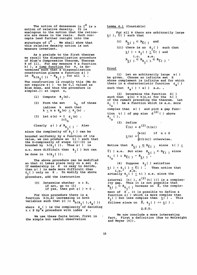
(3) Define

Lemma 4.1 (Constable)

t ( ) ~

since

n € Sif

satisfies

~a (n)

~(n) =d(t(n)") otherwise.

(i) R~( ). c Rt ( ) and

(ii) there is no ~ . ( ) such that

~(J_

) < ~j ( ) ~ t ( ) and

i.o. a.e.

~~( ). c R~. ( ). C Rt'( ) .J

Notice that R~( ).~ Rt () since

t( ) a.e. But also R!(). C Rt ( )~ i

o( ) E Rt ( ) - Ri ( ) ·

(4) Suppose t. (J

t ( ) < ~. ( ) < t( ) .- i.o. J · a~e.actually t. ( ) < t ( ) a. e. since the.

J -

interval [t ( ) I d (2) (t ( »] is a complex­ity gap. Thus it is not possible thatRt ( ).c R~. ( ) because on S, the comple-

- Jment of S I it is possible to define afunction ~( ) which is more complex than~. ( ) but less complex than t( ) • This

J -follows since on S, ~. ( ) « t( ) •

J -

Q.E.D.

ten) d(2) (t(n»

We now conclude a more interestingfact. First a definition (due to McCreightand Meyer [6]).

For all t ·there are arbitrarily large~( ), t( ) such that

(1) Let an arbitrarily large a()be given. Choose an infinite set Swhose complement is infinite and for whichthere is a characteristic function ~s( )

such that ~ s ( ) < a () a. e. •

(2) Determine the function d( )such that g(n) = h(n,n) for the h()of the remark preceding the theorem. Let~io () be a function which is a.e. more

complex than a() and pick a gap func­

tion t() of gap size d(2) ( ) abovet . ( ).~o

(0) Determine whether n € S,if not, go to (1)if yes, then put ~ ( ) = 0 •

be done in h(~j( ».The above procedure can be modified

so that it takes place only on a set s.If membership in S is easy to decide,then ~( ) is made more difficult than~. ( ) only on S. To modify the above

Jprocedure, add the instruction

For this procedure there is afunction h(n,m) increasing in bothvariables such that ~( )E Rh(t

j( ),t

s( »

where t ( ) is the complexity of decidingn € S bySa procedure with index s.

We use these facts below, first inthe simple but useful observation

(1) Compute tj(n).

(2) Form the set L n of those

indices k such thatk < n & ~k (n) < ~. (n) •

- J

( 3 ) Le t ~ (n) = L ~ i (n) •i€Ln

Clearly ~() t R~. ( ) • AlsoJ

since the complexity of ~j( ) can be

bounded uniformly by a function of itsvalue, we can produce an h( ) such thatthe t-complexity of steps (1)-(3) isbounded by h(t j ( ». Thus ~() is

a.e. more difficult than t. ( ) but canJ

As a prelude to the first theoremwe recall the diagonalization procedureof Blum's Compression Theorem, Theorem8 of [1]. For any measure ~ a functionh( ), a jump function for ~, is de­termined such that a diagonalizationconstruction places a function ~( )in Rh(~. ( » - R~. ( ) for all i.

J JThe construction is roughly this (We donot require ~() to be 0,1 valued asBlum does, and tbus the procedure issimpler.): at input n,

The notion of denseness in L~ is anotion of relative density. It isanalogous to the notion that the ration­als are dense in the reals. Such con­cepts lend further insight into the

structure of L~. We shall show thatthis relative density notion is notmeasure invariant.

15

Def. 4.2 similar to every measure.

A measure ~ is proper iff for all i,~

~ i ( e: R~. ( ) •~

We now conclude

Theorem 4.2 (Borodin)

Theorem 4.1 (Constable)

If ~ is proper, then the run-time

classes are not dense in L~.

There is a measure ~ for which therun-time classes are dense in ~ •

Proof

Def. 4.3

Proof

Two measures 4> and 4> are similarA

iff ~. ( ) = ~. () for all i suchJ. 1-

that range $. ( ) ~ {OJ •J.

We also need

to be a c.d. measure similar

L is both dense and run-

Take L

L. Then

Q.E.D.

Now we form, by theAmethods of

Theorem 3.3 , a measure ~ which makest( ) and t( ) into run-times of someL. ( ) below them. For instance, make the

1-

Li( ) of Theorem 3.3 a run-time of L i ()

rather than of itself.

We leave the details of this con­struction to the reader.

Q.E.D.

satisfies

Proof

Start with the dense measure L.Since the run-time classes are not densein L, there are arbitrarily large ~()

L Lt( ) such that Rt ( ).C R_ but no Li ( )- t ( )

to

Finally, we answer ~he questions leftopen from section III.

Theorem 4.3 (Constable)

There is a measure ~ for which E~

is dense but n4> is not.

time dense; and since L is c.~., the

run-time classes are dense in L

~n > t ,implies

The tape measure L is proper,thus the run-time classes are not dense inL although L is both dense and run-timedense. Is there then a measure ~ in

which the run-time classes are dense in L~?To answer this question, we refer tothe concept of similar measures intro­duced by McCreight & Meyer in [6].

4>i( ) ~ t( ).d () and t (

4>m{ ) = <P i { )

~a.e. R~(

and ~ is proper. Then ~ ( ) e: R~m '!1m

so there is a ~i() = ~m( ) with

Then by the definition of

) ,< g (~i ( » ~ g (t (» < t (~

C R~ (n

i.o. Hence ~m() contradicts Lemma 4.1

Q.E.D.

Let the d() of Lemma 4.1 bechosen larger than max {h(n,n),g(n)}for the g( ) of the Boun~ing Lemma.Construct t, t() and t( ) as in thepreceding lemma. Now suppose

~ ~ ~Rt ( C R~ ( ). C Rt (

- m

Det. 4.4

A set S of functions is classdetermining (C.D.) for 4> iff for allSUfficiently large t() there is ans( ) e: S such that Rt () = Rs ( ) •

A measure ~ is class determing iffS = {~. ( )} is c.d. Remark: McCreight

1-

& Meyer observe that no proper measurecan be c.d. But they prove the deepresult that there is a c.d. measure

Theorem~~.4 (Constable)

There is a measure ~ for which n~

is dense but L~ is not.

Proof

The plan of the proof is to proceedessentially as in Theorem 3.3 to construct

a measure ~ for which I~ is non-dense.By taking as the base measure for thisconstruction (the • of Theorem 3.3) the

16

(1) ~ ~ "tape in tape"RL . ( ) .c RL . ( )

,J. J

case.

(2) ~ ~ "new in tape·'R~. ( ) .c RL . ( ) ,

1 Jcase.

We will abbreviate these cases byusing the terms "new" and "tape" and byusing L i () for ~i() when ~i()

is a tape function, likewise for ~. ( ).J

Thus in summary form:

L LR~ ( ). c RL .( ).

i Jimplies

~) . c R~. ( ) , "tape in new"

J

R~.( CR~ )' "new in new"'i' ) • ~ • (.

1 J

~

Ri. (1

(4)

(3)

case

L We show how to construct anRL , ( ) .J

L ( such thatq

* 4> i ( ) < L ( ) < L. ( ) and. q - J1.0. a.e.

~. (n) < ~ (n)1 p

infinite subset of the integers), and if<P ( ) = <P ( ), then 4>, ( ) < 4> s ( ). If_s P ,. 1. i.o.~ ( ) is a tape complexity, then B

pfollows using <p ( ) for properness.

pHowever, if ~ ( ) is a new complexity

pfunction, then <p ( ) may not be in

p

Given A we know that there is a ~p(

such that ~ 1.' ( ) < ~ ( ) < L, ( ( i • e • ,i.o. P a7e. J

Sfor n € Sand S an

R~ c R.!~ i ( ) ~ --L j ( )

We shall consider in detail onlycase (2) which is the difficult case. Thegeneral principles will be clear from acareful examination of this case.

We show that A implies B, i.e.,

case •

Similar conventions will apply toother ~-complexity functions which arise,i.e., if ~ ( ) is introduced, then

pLpp ( ) and L~ ( ) are understood to be

defined. p

The strategy of the proof is to showthat (I) A implies B, and (II) (A impliesB) implies (A implies C).

We show each of these parts by exam­ining the four possible cases. Furtherspecial notation is used in the proofs,specifically:

let L ii () denote the tape complex­

ity function used as the base for construct­ing ~1' ( ), likewise for L" ( ) and ~,();

JJ J

let L~. ( ) and L~. ( ) denote1. J

respectively the tape complexities of thegap functions ~,() and ~. ( ) as defined

1 Jby the uniform procedure of Theorem 3.3(as modified slightly below) •

are(4) Both ~i ( ) and ~j (

new complexity functions.

~R~ . ( ) •

J

The difficult part of the proof isdemonstrating that n~ is dense. That L~is non-dense is proved exactly as inTheorem 3.3. We must show that Aimplies C. We distinguish four possibleways in which A can hold.

To simplify presentation of thisproof we use the following abbreviations:

~ ~A: R~. ( ). c R~. (

1 JL L

B. R~. ( ). c R~. ( )1 J ~ ~

C. ak such that R~. ( ).c R~ ( ).c1 k

(1) ~i() is a tape complexity

function (L. ( » and ~. ( ) is a~ J

tape complexity function (L j ( ».

(2) ~i() is a newly defined com­

plexity function in ~ (gap functionin L), but ~. ( ) is a tape com-

Jplexity function (L j ( ».

(3) ~. ( ) is a tape complexity1

function (L i ( » and ~j() is a

new complexity function.

measure L and by introducing severalspecial conditions on the· construction ofthe new complexity func·tions (gap functions

in L), it is possible to keep O~ dense.

Intuitively n~ remains dense becausewe scatter the new complexity functionsinto L sparsely enough that there aretape complexity functions of difficultfunctions between them. The specialconditions mentioned above are designedto insure the sparseness.

17

<I> s ( ) = <I> q ( ) implies ~ i ( ) < ~ s ( )

i.o. and ~J.' ( ) < L ( ) a.e. •- q

We distinguish two cases, p > iand p < i ,i.e., ~ ( ) constructedpafter ~. () or ~ ( ) constructed before

J. p~. ( ) • We also specify our first re­

J.striction on the construction of the newcomplexity functions.

Rl: If ~r(n) is constructed after

~s(n) and ~s(n) < ~r(n), then

we require that L~ (n) < ~r(n).s

It is easily seen that Rl doesnot alter the results of Theorem 3.3

Now ~or p > i we know ~i(n) <

L~. (n) < ~ (n) for n E s. Moreover weJ. p

recall from Theorem 3.3 that if ~s(n) =<P i ( ) , then L s ( ) > ~ i ( ) a. e. · We now

tkae ~q() to be the function obtained

by running in the minimum of L~. ( ) andJ.

L. ( ) • It is easy to see that L ( )J q

satisfies *

If P < i then we use a differenttrick. For this we need another restric­tion.

.R2 : ,Given the tape complexity Lk ( ),

define the associated gapfunction, Lk( ), so that it lies

lies above the tape complexity,

Lk , ( ), of the function 'k' (

obtained by applying the com­pression (or jump) procedure(of our Theorem 3.1) to Lk ( ).

Now we observe that if p < i and~J.' (n) < ~ (n), then L (n) must satisfyp pp~i(n) < Lpp(n) < ~p(n) , for otherwise

~i(n) would be forced above ~p(n) by

the gap defining procedure. If ~. ( ) <J.

~p( ) a.e., then Lpp ( ) suffices for

L ( ) and R2 is us~d to prove thatq

L () satisfies * If on the otherpphand ~ ( ) < ~. ( i.o., then we mustp J.use a more careful observation to dis­cover the right <P q (). We first need

another restriction.

R3: The gap size h() must be

18

taken to be a tape complexity­function.

Again the restriction does not negateany of the conclusions of Theorem 3.3since there is an increasing tape functionabove every recursive function.

Using this restriction we noticethat it is possible to decide whether

~. (n) < ~ (n) in less than h (2) (L (n) )J. P pp

tape. This fact is tedious to verify ~n

detail, but it follows informally becausei f ~. (n) < ~ (n), then ~. (n) < L (n) ,

J. P J. ppand the interval between Lii(n) and

Lpp(n) can be examined using only

h(2) (L (n» tape to determine whetherpp

~i(n) lies in it.

We then observe that h(2) (L (n» <pp

L. (n) for a.e.n. using RI and the factJ

that each new complexity function is atwo sided gap of size h() . We define~ ( ) as the function obtained by applyingqcompression to L () if ~. (n) < ~ (n)

pp J. Pand as <p. ( ) otherwise. It is easy to

Jshow that <p ( ) satisfies *. Thisqconcludes the proof that A implies B.

We now turn to showing (II) forcase (2), that (A implies B) implies(A implies C) • From A implies Band

L LA we conclude that R~. ( ).c RL . ( ) and

J. Jmoreover from * that

L L c rR~. ( ). C RL ( ) ~. ( ) •

J. q J

But because each new complexityfunction, ~ ( ), is a two sided gap,

pi • e ., if L k ( ) < ~p () a •e ., then

h(Lk ( » < ~p() a.e., we can construct

a function Lr ( ) such that

L ( ). < Lr ( ) ~ LJ. ( and

q J..O.

a.e. and

We do this by applying compressionto the part of L ( ) which is below

qL. ( ) . We have shown that this part car

Jbe recognized within L. ( so that the

Jresulting function ~r() satisfies the

above conditions. Thus

L L C RLR~ i ( ). C RL

q() L

j( ) •

[3] HartInanis, J. & Stearns, R.E. "Onthe Computational Complexity ofAlgorithms" Trans. AMS, 117, 5,1965, p.285-306.

Now it is easy to observe that this re­lationship carries over to ~. So

R~ R~ C R~ d A impliest. ( ). C L ( ). --L. ( ) , an1 q J

c.Q.E.D.

[4]

[5]

Hennie, F.C. & Stearns, R.E. "TwoTape Simulation of MultitapeMachines" JACM, 13, 4, 1966,p. 533-546. --

Kleene, S.C. Introduction toMathematics, Princeton, 1952.

[9] Young, Paul R. "Speed-Up byChanging the Order in which Setsare Enumerated" ACM Symposium onTheory of Computing, May 1967,p.89-92.

McCreight, E.M. & Meyer, A.R."Classes of Computable FunctionsDefined by Bounds on Computation"Proc. ACM S~osium on Theoryof Computing, Marina del Rey,1969, p.79-88.

Rogers, H. Theor¥ of RecursiveFunctions and E£ ective Com~uta­b!lity, New York, 1967.

[8] Rogers, H. "Godel Nwnberings ofPartial Recursive Functions"J. Symbolic Logic, 22, 3, 1958,p.33l-34l.

[7]

[6]

[1] Blum, M. "Machine-Independent Theoryof the Complexity of RecursiveFunctions" JACM, 14, 1967, p.322-36.

[2] Borodin, A. "Complexity Classes ofRecursive Functions and the Existenceof Complexity Gaps" Proc. ACMSymposium on the Theory of Computing,1969,p,.,~7-78•

References

A2knowledgement

We would like to thank Paul R.Yo~ng, who has independently constructed

a measure ~ for which neither L~ nor n~is dense, for the stimulation he providedin the writing of this paper.

19