QUIZ!!

T/F: Rejection Sampling without weighting is not consistent. FALSE T/F: Rejection Sampling (often) converges faster than Forward Sampling. FALSE T/F: Likelihood weighting (often) converges faster than Rejection Sampling. TRUE T/F: The Markov Blanket of X contains other children of parents of X. FALSE T/F: The Markov Blanket of X contains other parents of children of X. TRUE T/F: GIBBS sampling requires you to weight samples by their likelihood. FALSE T/F: In GIBBS sampling, it is a good idea to reject the first M<N samples. TRUE

Decision Networks: T/F: Utility nodes never have parents. FALSE T/F: Value of Perfect Information (VPI) is always non-negative. TRUE

1

CSE 511a: Artificial IntelligenceSpring 2013

Lecture 19: Hidden Markov Models

04/10/2013

Robert Pless

Via Kilian Q. Weinberger, slides adapted from Dan Klein – UC Berkeley

Recap: Decision Diagrams

Weather

Forecast

Umbrella

U

A W U

leave sun 100

leave rain 0

take sun 20

take rain 70

W P(W)

sun 0.7

rain 0.3

F P(F|rain)

good 0.1

bad 0.9

F P(F|sun)

good 0.8

bad 0.2

Example: MEU decisions

4

Weather

Forecast=bad

Umbrella

U

A W U(A,W)

leave sun 100

leave rain 0

take sun 20

take rain 70

W P(W|F=bad)

sun 0.34

rain 0.66

Umbrella = leave

Umbrella = take

Optimal decision = take

Value of Information Assume we have evidence E=e. Value if we act now:

Assume we see that E’ = e’. Value if we act then:

BUT E’ is a random variable whose value is unknown, so we don’t know what e’ will be.

Expected value if E’ is revealed and then we act:

Value of information: how much MEU goes upby revealing E’ first:

VPI == “Value of perfect information”

VPI Example: Weather

6

Weather

Forecast

Umbrella

U

A W U

leave sun 100

leave rain 0

take sun 20

take rain 70

MEU with no evidence

MEU if forecast is bad

MEU if forecast is good

F P(F)

good 0.59

bad 0.41

Forecast distribution

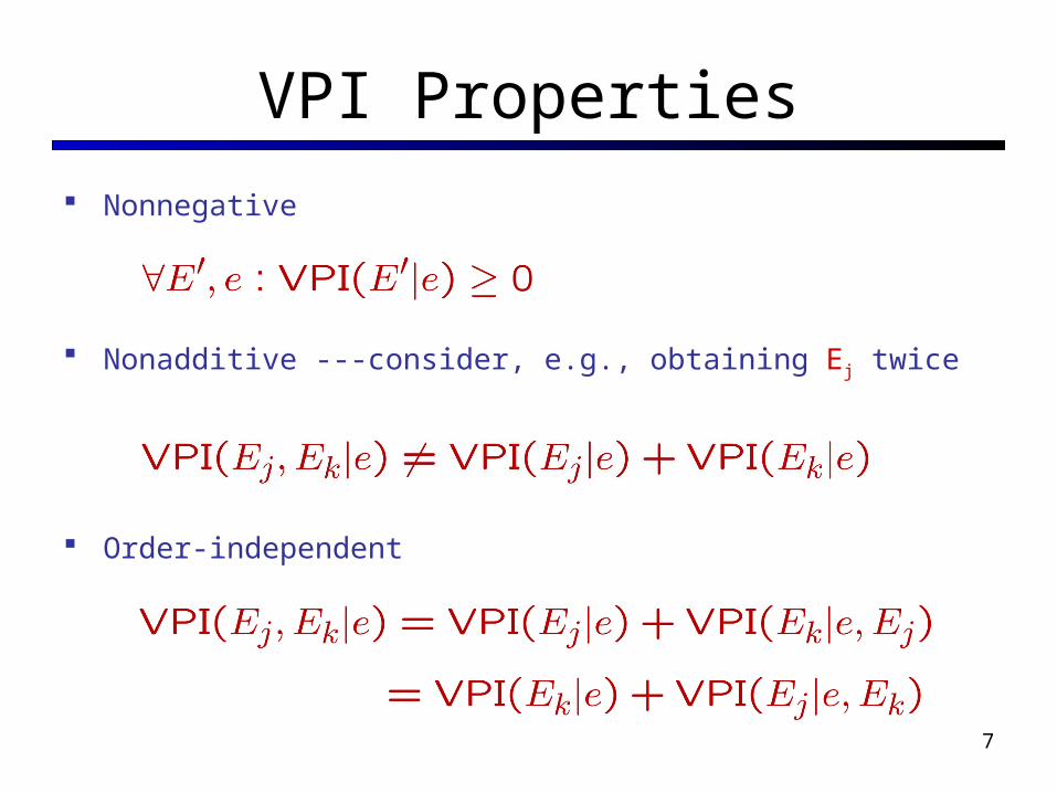
VPI Properties

Nonnegative

Nonadditive ---consider, e.g., obtaining Ej twice

Order-independent

7

8

Now for something completely different

9

“Our youth now love luxury. They have bad manners, contempt for authority; they show disrespect for their elders and love chatter in place of exercise; they no longer rise when elders enter the room; they contradict their parents, chatter before company; gobble up their food and tyrannize their teachers.”

10

“Our youth now love luxury. They have bad manners, contempt for authority; they show disrespect for their elders and love chatter in place of exercise; they no longer rise when elders enter the room; they contradict their parents, chatter before company; gobble up their food and tyrannize their teachers.”

– Socrates 469–399 BC

11

Adding time!

Reasoning over Time

Often, we want to reason about a sequence of observations Speech recognition Robot localization User attention Medical monitoring

Need to introduce time into our models Basic approach: hidden Markov models (HMMs) More general: dynamic Bayes’ nets

12

13

Markov Model

Markov Models

A Markov model is a chain-structured BN Each node is identically distributed (stationarity) Value of X at a given time is called the state As a BN:

….P(Xt|Xt-1)…..

Parameters: called transition probabilities or dynamics, specify how the state evolves over time (also, initial probs)

X2X1 X3 X4

Conditional Independence

Basic conditional independence: Past and future independent of the present Each time step only depends on the previous This is called the (first order) Markov property

Note that the chain is just a (growing) BN We can always use generic BN reasoning on it if we

truncate the chain at a fixed length

X2X1 X3 X4

15

Example: Markov Chain

Weather: States: X = {rain, sun} Transitions:

Initial distribution: 1.0 sun What’s the probability distribution after one step?

rain sun

0.9

0.9

0.1

0.1

This is a CPT, not a

BN!

16

Mini-Forward Algorithm

Question: What’s P(X) on some day t? An instance of variable elimination!

sun

rain

sun

rain

sun

rain

sun

rain

Forward simulation18

Example

From initial observation of sun

From initial observation of rain

P(X1) P(X2) P(X3) P(X)

P(X1) P(X2) P(X3) P(X) 19

Stationary Distributions

If we simulate the chain long enough: What happens? Uncertainty accumulates Eventually, we have no idea what the state is!

Stationary distributions: For most chains, the distribution we end up in is

independent of the initial distribution Called the stationary distribution of the chain Usually, can only predict a short time out

22

Hidden Markov Model

Hidden Markov Models

Markov chains not so useful for most agents Eventually you don’t know anything anymore Need observations to update your beliefs

Hidden Markov models (HMMs) Underlying Markov chain over states S You observe outputs (effects) at each time step As a Bayes’ net:

X5X2

E1

X1 X3 X4

E2 E3 E4 E5

Example

An HMM is defined by: Initial distribution: Transitions: Emissions:

Ghostbusters HMM

P(X1) = uniform

P(X|X’) = usually move clockwise, but sometimes move in a random direction or stay in place

P(Rij|X) = same sensor model as before:red means close, green means far away.

1/9 1/9

1/9 1/9

1/9

1/9

1/9 1/9 1/9

P(X1)

P(X|X’=<1,2>)

1/6 1/6

0 1/6

1/2

0

0 0 0X5

X2

Ri,j

X1 X3 X4

Ri,j Ri,j Ri,j

E5

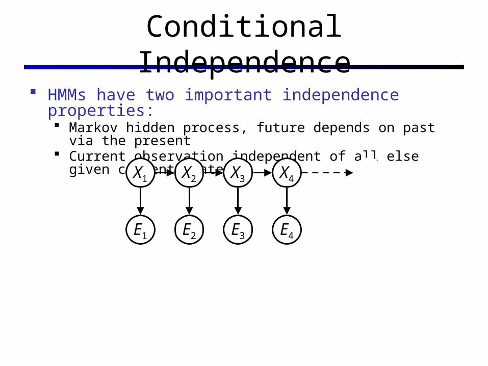
Conditional Independence

HMMs have two important independence properties: Markov hidden process, future depends on past via the present Current observation independent of all else given current state

Quiz: does this mean that observations are independent given no evidence? [No, correlated by the hidden state]

X5X2

E1

X1 X3 X4

E2 E3 E4 E5

Real HMM Examples

Speech recognition HMMs: Observations are acoustic signals

(continuous valued) States are specific positions in specific

words (so, tens of thousands)

Machine translation HMMs: Observations are words (tens of thousands) States are translation options

Robot tracking: Observations are range readings

(continuous) States are positions on a map (continuous)

Filtering / Monitoring

Filtering, or monitoring, is the task of tracking the distribution B(X) (the belief state) over time

We start with B(X) in an initial setting, usually uniform

As time passes, or we get observations, we update B(X)

The Kalman filter was invented in the 60’s and first implemented as a method of trajectory estimation for the Apollo program

Example: Robot Localization

t=0Sensor model: never more than 1 mistake

Motion model: may not execute action with small prob.

10Prob

Example from Michael Pfeiffer

Example: Robot Localization

t=1

10Prob

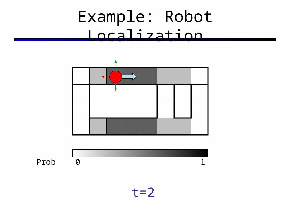
Example: Robot Localization

t=2

10Prob

Example: Robot Localization

t=3

10Prob

Example: Robot Localization

t=4

10Prob

Example: Robot Localization

t=5

10Prob

Inference Recap: Simple Cases

E1

X1 X2X1

Passage of Time

Assume we have current belief P(X | evidence to date)

Then, after one time step passes:

Or, compactly:

Basic idea: beliefs get “pushed” through the transitions With the “B” notation, we have to be careful about what time step

t the belief is about, and what evidence it includes

X2X1

Example: Passage of Time

As time passes, uncertainty “accumulates”

T = 1 T = 2 T = 5

Transition model: ghosts usually go clockwise

Observation Assume we have current belief P(X | previous evidence):

Then:

Or:

Basic idea: beliefs reweighted by likelihood of evidence

Unlike passage of time, we have to renormalize

E1

X1

Example: Observation

As we get observations, beliefs get reweighted, uncertainty “decreases”

Before observation After observation

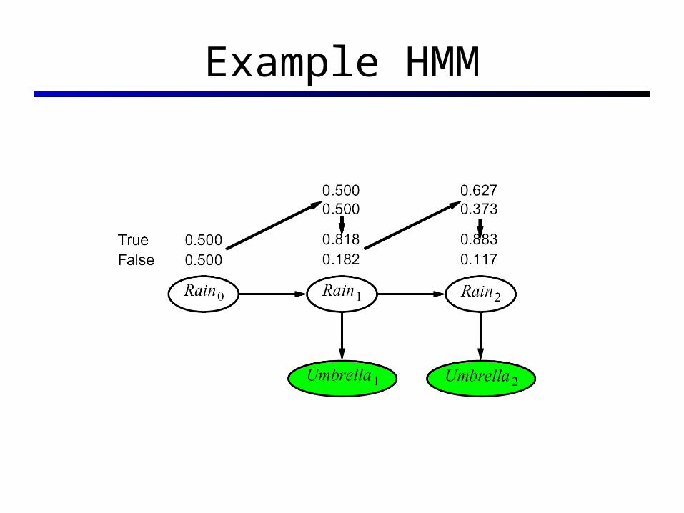
Example HMM

The Forward Algorithm

We are given evidence at each time and want to know

We can derive the following updates

We can normalize as we go if we

want to have P(x|e) at each time

step, or just once at the end…

Online Belief Updates

Every time step, we start with current P(X | evidence) We update for time:

We update for evidence:

The forward algorithm does both at once (and doesn’t normalize) Problem: space is |X| and time is |X|2 per time step

X2X1

X2

E2

44

Next Lecture: Sampling! (Particle Filtering)