Sampling Distributions

The sampling distribution of a sample function, say x̄, calculated from a random

sample of size n is simply the probability distribution of x̄ (obtained from all possible

samples of n observations from a population with mean µ and variance σ2).

Central Limit Theorem.

If n is large, the sampling distribution of x̄ will be approximately a normal distru-

bution with mean µx̄ = µ and standard deviation σx̄ = σ√n. The standard deviation

σx̄ is often referred to as the standard error of the sample mean x̄.

1

Example.

According to AAA, the average daily meal and lodging costs for a family of four

is $213. Assume that the standard deviation of such cost is $15. Consider a random

sample of 36 families of four and their travel expenses. Find the ptobability that sample

mean exceeds $200.

Example.

The weight of corn chips dispensed into a 10-ounce bag by the dispensing machine

has been identified as possessing a normal distribution with a mean of 10.5 ounces and

a standard deviation of .2 ounces. Suppose 100 bags of chips were randomly selected

from this dispensing machine. Find the probability that the sample mean weight of

these 100 bags exceeded 10.45 ounces.

Example.

The amount of time it takes a student to walk from her home to class has a skewed

right distribution with a mean of 16 minutes and a standard deviation of 1.6 minutes. If

data were collected from 36 randomly selected walks, describe the sampling distribution

of x̄, the sample mean time.

2

True or False: The Central Limit Theorem guarantees that the population is

normal whenever n is sufficiently large.

True or False: The Central Limit Theorem guarantees an approximately normal

sampling distribution for the sample mean for large sample sizes, so no knowledge about

the distribution of the population is necessary for large-sample confidence intervals to

be valid.

3

Inference Based on a Single Sample

A 100(1−α)% confidence interval for µ is a formula that gives an interval for each

sample of n observations with the property that, in repated sampling of n observations,

100(1-α)% of all intervals enclose µ. In other words, the formula is 100(1-α)% accu-

rate in the sense that 100(1-α)% of the time, in repeated sampling, the formula gives

intervals that enclose µ.

The fraction (1−α) is called confidence coefficient and 100(1−α)% is often referred

to as confidence level.

1. Large Sample 100(1-α)% Confidence Interval for µ:

L = x̄− Zα/2σ√n

, U = x̄ + Zα/2σ√n

Here Zα/2 is obtained from standard normal distribution table so that the area

to the left of Zα/2 is equal to 1 − α/2. If the population standard deviation

σ is unknown, it is replaced by s, the sample standard deviation to obtain an

approximate confidence interval.

4

Example. How much money does the average professional football fan spend on food

at a single football game? The question was posed to 40 randomly selected football

fans. The sampled results show that the sample mean and standard deviation were

x̄ = $52 and s = $17.50, respectively.

(a) Find a 95% confidence interval for the true mean µ.

(b) Which of the following interpretations is correct for your interval in (a)?

(i) 95% of the population values will fall in the interval.

(ii) 95% of the similarly constructed intervals would contain the value of the sample

mean.

(iii) The probability that the population mean falls in any confidence interval con-

structed is 0.95.

(iv) In repeated sampling, 95% of the intervals constructed would contain µ.

Example. Each in a sample of 65 low-income children was administered the Commu-

nicative Development Inventory (CDI) exam. The sentence complexity scores had a

mean of 7.62 and a standard deviation of 8.91. Construct a 90% confidence interval for

the mean sentence complexity score of all low-income children.

5

2. Small Sample 100(1-α)% Confidence Interval for µ (assuming that the random

sample is selected from normal distribution):

L = x̄− (tα/2,n−1)s√n

, U = x̄ + (tα/2,n−1)s√n

Here tα/2,n−1 is obtained from the t-dsitribution table so that the area to the right

hand side of tα/2,n−1 is α/2. The formula requires that the sampled population

be normal.

Example. A meteorologist wishes to estimate the mean amount of snowfall per year in

Spokane, Washington. A random sample of the recorded snowfall for 20 years produces

a sample mean equal to 54 inches and standard deviation of 9 inches. Estimate the

true mean amount of snowfall in Spokane using a 90% confidence interval.

Example. Pulse rate is an important measure of the fitness of a person’s cardiovascular

system. A random sample of 5 U.S adult males who jog at least 15 miles per week had

had the following pulse rates per minutes.

54 50.5 50.8 53 52.5

(x̄ = 52.16, s2 = 2.203)

Find a 95% confidence interval for the mean pulse rate of all U.S. adult males who jog

at least 15 miles per week.

6

3. Large Sample 100(1-α)% Confidence Interval for the binomial proportion p.

L = p̂− Zα/2

√p̂(1− p̂)

n, U = p̂ + Zα/2

√p̂(1− p̂)

n

Here Zα/2 is obtained from standard normal distribution table so that the area to

the left of Zα/2 is equal to 1− alpha/2.

Note. The sample size n is considered large if p̂± 3√

p̂(1− p̂)/n falls between 0 and 1.

Example. A university dean is interested in determining the proportion of students who

receive some sort of financial aid. Rather than examine the records for all students, the

dean randomly selects 200 students and finds that 118 of them are receiving financial

aid. Use a 90% confidence interval to estimate the true proportion of students on

financial aid.

Example. Suppose that in a random sample of 200 Americans, 85 were victims of a

crime. Estimate the true proportion of Americans who were victims of a crime using a

95% confidence confidence interval.

7

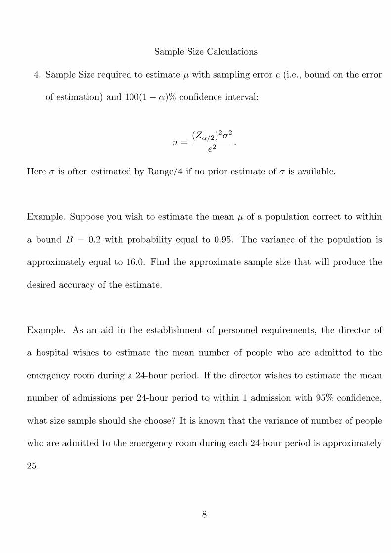
Sample Size Calculations

4. Sample Size required to estimate µ with sampling error e (i.e., bound on the error

of estimation) and 100(1− α)% confidence interval:

n =(Zα/2)2σ2

e2.

Here σ is often estimated by Range/4 if no prior estimate of σ is available.

Example. Suppose you wish to estimate the mean µ of a population correct to within

a bound B = 0.2 with probability equal to 0.95. The variance of the population is

approximately equal to 16.0. Find the approximate sample size that will produce the

desired accuracy of the estimate.

Example. As an aid in the establishment of personnel requirements, the director of

a hospital wishes to estimate the mean number of people who are admitted to the

emergency room during a 24-hour period. If the director wishes to estimate the mean

number of admissions per 24-hour period to within 1 admission with 95% confidence,

what size sample should she choose? It is known that the variance of number of people

who are admitted to the emergency room during each 24-hour period is approximately

25.

8

5. Sample Size required to estimate the binomial proportion p with sampling error e

(i.e., bound on the error of estimation) and 100(1− α)% confidence interval:

n =(Zα/2)2p(1− p)

e2.

Use 0.5 for p if no prior estimate of p is available.

Example. A university dean is interested in determining the proportion of students

who receive some sort of financial aid. If the dean wanted to estimate the proportion

of all students receiving financial aid to within 3% with 95% confidence, how many

students would need to be sampled?

9

Review Exercises

1. A local men’s clothing store is being sold. The buyers are trying to estimate

the percentage of items that are outdated. They will randomly sample among its

100,000 items in order to determine the proportion of merchandise that is outdated.

The current owners have never determined their outdated percentage and can not

help the buyers. Approximately how large a sample do the buyers need in order

to insure that they are 99% confident that the margin of error is within 4%?

2. A university is considering a change in the way students pay for their education.

Presently, the students pay $16 per credit hour. The university is contemplating

charging each student a set fee of $240 per quarter, regardless of how many credit

hours each takes. To see if this proposal would be economically feasible, the

university would like to know how many credit hours, on the average, each student

takes per quarter. A random sample of 250 students yields a mean of 14.1 credit

hours per quarter and a standard deviation of 2.8 credit hours per quarter. Suppose

the administration wanted to estimate the mean to within 0.3 credit hours at 95%

reliability. How large a sample would they need to take?

10

3. An article in a Florida newspaper reports on the topics that teenagers most want

to discuss with their parents. The findings, the results of a poll, showed that 30%

would like to talk about religion. This percentage was based on a national sampling

of 505 teenagers. Estimate the proportion of all teenagers who want more family

discussions about religion. Use a 90% confidence level.

4. The increasing cost of health care is an important issue today. Suppose that a

random sample of 25 small companies that offer paid health insurance as a benefit

was selected. The mean health insurance cost per worker per month was $124,

and the standard deviation was $30. Construct a 95% confidence interval for the

average health cost per worker per month for all small companies.

11

For the question below, answer True or False

1) As the sample size taken gets larger, the standard error of the mean gets larger

as well.

2) The standard error of the mean is equal to sigma, the standard deviation of the

population.

3) One way of reducing the width of a confidence interval is to reduce the confidence

level.

4) One way of reducing the width of a confidence interval is to reduce the size of

the sample taken.

5) If no estimate of p exists when determining the sample size, we can use .5 in

the formula to get a value for n.

12

Elements of a Test of Hypothesis

1. Null Hypothesis (H0) - A statement about the values of population parameters

which we accept until proven false.

2. Alternative or Research Hypothesis (Ha)- A statement that contradicts the null

hypothesis. It represents researcher’s claim about the population parameters. This

will be accepted only when data provides sufficient evidence to establish its truth.

3. Test Statistic - A sample statistic (often a formula) that is used to decide whether

to reject H0.

4. Rejection Region- It consists of all values of the test statistic for which H0 is rejected.

This rejection region is selected in such a way that the probability of rejecting true H0

is equal to α (a small number usually 0.05). The value of α is referred to as the level

of significance of the test.

5. Assumptions - Statements about the population(s) being sampled.

6. Calculation of the test statistic and conclusion- Reject H0 if the calculated value of

the test statistic falls in the rejection region. Otherwise, do not reject H0.

7. P-value or significance probability is defined as proportion of samples that would

be unfavourable to H0 (assuming H0 is true) if the observed sample is considered

unfavourable to H0. If the p-value is smaller than α, then reject H0.

13

Remark:

1. If you fix α = 0.05 for your test, then you are allowed to reject true null hypothesis

5% of the time in repeated application of your test rule.

2. If the p-value of a test is 0.20 (say) and you reject H0 then, under your test rule,

20% of the time you would reject true null hypothesis.

14

1. Large sample (n > 30) test for H0 : µ = µ0 (known).

Z =x̄− µ0

σ√n

Example. A study reported in the Journal of Occupational and Organizational Psy-

chology investigated the relationship of employment status to mental health. Each of a

sample of 49 unemployed men was given a mental health examination using the General

Health Questionnaire (GHQ). The GHQ is widely recognized measure of present men-

tal health , with lower values indicating better mental health. The mean and standard

deviation of the GHQ scores were x̄ = 10.94 and s = 5.10, respectively.

(a). Specify the appropriate null and alternative hypothesis if we wish to test the

research hypothesis that the mean GHQ score for all unemployed men exceeds 10.

Is the test one-tailed or two-tailed?

(b). If we specify α = 0.05, what is the appropriate rejection region for this test?

(c). Conduct the test, and state your conclusion clearly in the language of this exercise.

Find the p-value of the test.

15

Example. A consumer protection group is concerned that a ketchup manufacturer is

filling its 20-ounce family-size containers with less than 20 ounces of ketchup. The

group purchases 49 family-size bottles of this ketchup, weigh the contents of each, and

finds that the mean weight is 19.86 ounces, and the standard deviation is equal to 0.22

ounces.

(a). Do the data provide sufficient evidence for the consumer group to conclude that

the mean fill per family-size bottle is les than 20 ounces? Test using α = 0.05.

(b). Find the p-value of the your test in part (a).

16

Example. State University uses thousands of fluorescent light bulbs each year. The

brand of bulb it currently uses has a mean life of 900 hours. A manufacturer claims

that its new brands of bulbs, which cost the same as the brand the university currently

uses, has a mean life of more than 900 hours. The university has decided to purchase

the new brand if, when tested, the test evidence supports the manufacturer’s claim at

the .10 significance level. Suppose 99 bulbs were tested with the following results: x̄ =

919 hours, s = 86 hours. Find the rejection region for the test of interest to the State

University.

17

2. Small sample (n ≤ 30) test for H0 : µ = µ0 (known).

t =x̄− µ0

s√n

This test requires that the sampled population is normal.

Example. A random sample of n observations is selected from a normal population

to test the null hypothesis that µ = 10. Specify the rejection region for each of the

following combinations of Ha, α, and n.

(a). Ha : µ 6= 10, α = 0.01, n = 14.

(b). Ha : µ < 10, α = 0.025, n = 26.

18

Example. According to advertisements, a strain of soybeans planted on soil prepared

with a specified fertilizer treatment has a mean yield of 475 bushels per acre. Twenty

farmers who belong to a cooperative plant the soybeans. Each uses a 40-acre plot and

records the mean yield per acre. The mean and variance for the sample of 20 farms are

x̄ = 462 and s2 = 9070. Specify the null and alternative hypothesis used to determine

if the mean yield for the soybeans is different than advertised.

19

Example. A psychologist was interested in knowing whether male heroin addicts’ as-

sessments of self-worth differ from those of the general male population. On a test

designed to measure assessment of self-worth, the mean score for males from the gen-

eral population was found to be equal to 48.6. A random sample of 25 scores achieved

by heroin addicts yielded a mean of 44.1 and a standard deviation of 6.2. Do the

data indicate a difference in assessment of self-worth between male heroin addicts and

general male population? Test using α = 0.01.

20

3. Large sample test for H0 : p = p0 (known).

Z =p̂− p0√p0(1−p0)

n

For this test, sample size is considered large if p0 ± 3√

p0(1−p0)n falls between 0 and 1.

Example. The National Science Foundation, in a survey of 2,237 engineering graduate

students who earned their Ph.D. degrees, found that 607 were U.S. citizens; the majority

(1,630) of the Ph.D degrees were awarded to foreign nationals. Conduct a test to

determine whether the true percentage of engineering Ph.D. degrees awarded to foreign

nationals exceeds 50%. Use α = 0.01.

21

Example. The business college computing center wants to determine the proportion

of business students who have personal computers (PC’s) at home. If the proportion

exceeds 30 percent, then the lab will scale back a proposed enlargement of its facilities.

Suppose 250 business students were randomly sampled and 85 have personal computers

at home. Conduct a test to see if the scale back of the proposed enlargement of its

facilities is needed. Use α = 0.05.

22

Example. A method currently used by doctors to screen women for possible breast

cancer fails to detect cancer in 15% of the women who actually have the disease. A

new method has been developed that researchers hope will be able to detect cancer

more accurately. A random sample of 70 women known to have breast cancer were

screened using the new method. Of these, the new method failed to detect cancer

in six. Specify the null and alternative hypothesis that the researchers wish to test.

Calculate the test statistic, determine the rejection region if α = 0.05, find the p-value,

and state the conclusion clearly in the language of this exercise.

23

Example. The Midwest Organization of Retired Oncologists and Neurologists (M.O.R.O.N.)

has recently taken flack from some of its members regarding the poor choice of the orga-

nization’s name. The association bylaws require that more than 60% of the organization

must approve a name change. Rather than convene a meeting, it is first desired to use a

sample to determine if a meeting is necessary. A random sample of 60 of M.O.R.O.N.’s

members were asked if they want M.O.R.O.N. to change its name. Forty-five of the

respondent’s said ”yes.” Find the p-value for the desired test of hypothesis.

24

Example. Increasing numbers of businesses are offering child-care benefits for their

workers. However, one union claims that more than 80% of firms in the manufacturing

sector still do not offer any child-care benefits to their workers. A random sample of 480

manufacturing firms is selected, and only 27 of them offer child-care benefits. Specify

the rejection region that the union will use when testing at alpha = .05. Suppose the

p-value for this test was reported to be p = .1113. State the conclusion of interest to

the union. Use alpha = .10.

25