QuECT: A New Quantum Programming Paradigm - Indian Statistical

QuECT: A New Quantum Programming

Paradigm

Arnab Chakraborty

Applied Statistics Unit

Indian Statistical Institute

203, B T Road

Kolkata, India 700108

Phone: 91-33-2334-0337

[email protected]

Abstract

Quantum computation constitutes a rapidly expanding subfield of com-

puter science. Development quantum algorithms is facilitated by the avail-

ability of efficient quantum programming languages, and a plethora of

approaches has been already suggested in the literature, ranging from

GUI-based simple tools to elaborate standalone programming languages.

In this paper we propose a novel paradigm called Quantum Embeddable

Circuit Technique (QuECT) that allows a programmer to embed a circuit

diagram in a classical “host” language. The paradigm can be implemented

in any modern classical language. A prototype has been developed by the

author using Java.

1

1 Introduction

Quantum computation is a rapidly developing field, and even though ac-

tual quantum computers are yet to be constructed in a large scale, many

quantum computing algorithms have already appeared in the literature.

One needs some quantum programming language to present these algo-

rithms to a quantum computer (or a simulator). A variety of approaches

have been suggested in the literature to this end. These range from

drag-and-drop graphical interfaces to quantum assembly languages. Most

textbooks like to present quantum algorithms in the form of “circuit di-

agrams.” All the graphical approaches to quantum programming rely on

these circuit diagrams. Its intuitive nature notwithstanding, this ubiqui-

tous technique is not easily amenable to standard programming constructs

like conditional jumps and loops. In this paper we propose a new quantum

programming paradigm called Quantum Embeddable Circuit Tech-

nique (QuECT) that combines the power of circuit diagram and yet

allows the traditional control structures. It enhances an existing classical

language to handle quantum circuit diagram embedded in it. The au-

thor’s implementation uses Java as the classical “host” language, but the

same idea carries over directly to any other language (compiled/byte code

compiled/interpreted). The QuECT paradigm is equally applicable for a

real quantum computer (when one is constructed) as it is for a simulator.

It is expected that this paradigm will help traditional programmers to

pick up quantum computing more easily.

At this point the reader may like to take a look at a simple example

of the QuECT approach given in section 4. The layout of the paper

is as follows. Section 2 gives a concise summary of the basic notions

of quantum computing. Our exposition loosely follows that of [14]. In

section 3 we review the quantum programming paradigms in existence.

The section after that is devoted to the details of the QuECT paradigm.

2

Section 5 shows the paradigm in action, where we demonstrate QuECT

implementation of some standard quantum algorithms. Some practical

issues about compiling a QuECT program may be found section 6. A

literate programming descrition of our Java implementation is given in

the appendix.

2 Basic ideas

2.1 Qubits

The most fundamental building block of quantum computing is a qubit,

which is often considered as the quantum analog of a bit, and hence its

name. This analogy, however, has its pitfalls, and for a rigorous under-

standing one should better remember a qubit as a nonzero element of C2,

identified up to multiples. Thus, (1, i) is a qubit, and (1, 2+ i) is another.

The qubit (i,−1) is actually the same as (1, i), since these are multiples

of each other. The two qubits (1, 0) and (0, 1) are special, and have the

names |0〉 and |1〉, respectively.

By a k-qubit system we shall understand a nonzero element of C2

k

.

A 1-qubit system is the same as a single qubit. However, for general k a

k-qubit system is not the same as a collection of k qubits. Two k-qubit

systems are considered the same if they are (nonzero) multiples of each

other.

Since we are working with vectors and matrices of size 2k, it is obvious

that the sizes are going to explode pretty soon even for a modest k. While

it is not supposed to pose a problem to a computer with quantum hard-

ware, it is nevertheless difficult for a human programmer to keep track of

such large vectors and matrices. The concept of factorization helps us here

by expressing a large vector as tensor product (also known as Kronecker

product) of shorter vectors. This allows us to work with the shorter vec-

tors separately, combining the results at the very end, if necessary. For

3

example, it may be possible to express a n-qubit system (consisting of

2n complex numbers) as a tensor product of k systems of sizes n1, ..., nk

(whereP

ni = n) requiring a total of onlyP

2ni complex numbers).

However, not all quantum systems admit a factorization. If a n-qubit

system cannot be factored, then we say that the n qubits are entangled.

Entangled qubits give the main power to quantum programming, and also

stand as the main hurdle for a classical programmer aspiring to write a

quantum program.

2.2 Quantum gates

The second most important concept in quantum computing is that of

quantum gates, which are unitary matrices with complex entries. We shall

think of a k-qubit system as a column vector of length 2k, and a quantum

gate as a unitary matrix of size 2k multiplying it from the left. From the

viewpoint of a quantum programmer these are of two types. First, there

are some commonly used operators (e.g., Hadamard, Pauli’s X, Y, Z etc).

Then there are the operators specially crafted for some specific algorithm.

The most prominent example of the later type is a “quantum wrapper”

that packages a classical function f : {0, 1}m → {0, 1}n into a unitary

matrix Uf of order 2m+n as follows.

To find the (i, j)-th entry of Uf we first express i and j in binary

using m + n bits. Then we split each of them into two parts: the x-part

consisting of the most significant m bits, and the y-part consisting of the

least significant n bits. Let these be denoted by ix, iy, jx and jy . Then

U(f)ij =

8

>

<

>

:

1 if ix = jx and f(ix) = iy ⊕ jy

0 otherwise.

It is not difficult to see that each row and each column of U(f) has exactly

a single 1, and so U(f) is unitary.

4

2.3 Measurement

The third important concept in quantum computing is that of measure-

ment. While it is standard to treat measurement as a Hermitian operator,

we shall restrict ourselves to the most frequently used form, viz., measure-

ment of one or more qubits in a multi-qubit system. If we measure p given

qubits in a k-qubit system then we shall observe a random variable which

takes values 0, 1, ..., 2p−1 (or, equivalently, the corresponding bit patterns

of length p). Quantum physics dictates that the probability of observing

a given bit pattern b isP

′ |zi|2

‖z‖2,

where the numerator sum is for those i’s only whose binary representations

have the pattern b in the positions of the qubits being measured. For

example, if we measure qubits at positions 0 and 2 in a 3-qubit system

containing the value (z0, ..., z7), we shall observe 0 or 1 or 2 or 3 with the

probabilities

P (0) = P (00) =|z000|

2 + |z010|2

‖z‖2,

P (1) = P (01) =|z001|

2 + |z011|2

‖z‖2,

P (2) = P (10) =|z100|

2 + |z110|2

‖z‖2,

P (3) = P (11) =|z101|

2 + |z111|2

‖z‖2.

Here z000 means z0, z001 means z1, and so on. Also the bits at positions

0 and 2 are underlined in the right hand sides for ease of comparison.

The process of measurment also changes the contents of the multi-qubit

system. If the output is the bit pattern b, then the contents of the multi-

qubit system changes from z to w where

wi =

8

>

<

>

:

zi if i has pattern b in the measured positions

0 otherwise.

5

The fact that a quantum measurement potentially changes the un-

derlying quantum system is a main distinguishing feature of quantum

systems over classical ones. However, in a typical quantum algorithm

the measurement comes at the very end. So we do not care about the

fate of the system once the measurement is over. However the way a

measurement affects the contents of a quantum system has the following

theoretical implication which indirectly helps a quantum programmer.

Suppose that we are working with a k-qubit system. Let A, B be

two disjoint, nonempty subsets of {0, ..., k − 1}. Then all the following

measurement operations will produce identically distributed outputs:

1. First measure the qubits at positions A, then measure those at po-

sitions B.

2. Measure the qubits at positions A ∪ B.

This observation allows us to combine all the measurements at the end

of an algorithm into a single mesaurement.

2.4 Quantum circuits

A quantum algorithm, in its barest form, consists of

1. a multi-qubit system with some given classical initial value, (i.e., a

tensor product of |0〉’s and |1〉’s),

2. an ordered list of quantum gates that act on the system in that

order,

3. measurements of some qubits at the very end.

Usually the quantum gates are complicated, huge matrices, made by

taking tensor products of smaller matrices. An actual quantum computer

will have no problem in computing the effect of applying such gates, but a

human programmer always finds it easier to specify a huge gate in terms

6

of the constituent smaller gates. The quantum circuit diagram is the most

popular way to achieve this.

The evolution of a k-qubit system is shown in a quantum circuit as k

parallel lines. Roughly speaking, these lines are like k wires each carrying

a single qubit1. The left hand circuit diagram in Fig 1, for example,

represents a 1-qubit system initially storing |0〉, and being acted upon by

a quantum gate A (which is a 2 × 2 unitary matrix).

A B|0〉 |1〉

|0〉

Fig 1: Two simple quantum circuits

The right hand circuit diagram represents a 2-qubit system starting

with the value

|1〉 ⊗ |0〉 =

2

6

6

6

6

6

6

6

4

0

0

1

0

3

7

7

7

7

7

7

7

5

and being acted upon by a quantum gate B which must be a 22 × 22

unitary matrix. The result may not be factorizable as a tensor product

of two qubits, in which case it is meaningless to talk about the values of

the individual output lines.

1This analogy is not entirely correct in presence of possible entanglement, as we shall see

soon.

7

The following circuit shows a 3-qubit system starting with the content

|0〉 ⊗ |1〉 ⊗ |0〉 =

2

6

6

6

6

6

6

6

6

6

6

6

6

6

6

6

6

6

6

6

6

6

4

0

0

1

0

0

0

0

0

3

7

7

7

7

7

7

7

7

7

7

7

7

7

7

7

7

7

7

7

7

7

5

.

A

B

|0〉

|1〉

|0〉

Fig 2: An example of entanglement

Then it is acted upon by the 23 × 23 unitary matrix

A ⊗ B.

The lower 2 qubits are possibly entangled together, however they are

not entangled with the top qubit. This is shown using a broken ellipse

(which is not part of a standard circuit diagram).

Fig 3 presents a more complicated example that also demonstrates a

pitfall.

A

Stage 2Stage 1

B

|0〉

|0〉

|1〉

CFig 3: A more complicated circuit

8

It would be wrong to think that the quantum gate C acts upon the

top two qubits. This is because the middle qubit actually does not exist

separately after stage 1, thanks to the possible entanglement introduced

by B. Thus the naive interpretation that each line is like a wire carrying a

single qubit does not hold any more. The unitary matrix that is depicted

by this diagram is actually

(C ⊗ I2)(A ⊗ B), (*)

where I2 denotes identity matrix of order 2 (corresponding to the bottom

line “passing through” stage 2). This circuit also has some measurement

symbols. Here we are measuring the two extreme qubits. The overall

circuit denotes a quantum function from {0, 1}3 to {0, 1}2.

The usefulness of circuit diagrams to represent quantum algorithms

stems from the following reasons.

1. It allows one to work with just k lines even when the underlying

system has dimension 2k.

2. The quantum gates can be constructed easily out of component gates

suppressing cumbersome expressions like (*) involving tensor prod-

ucts and identity matrices.

The chief drawbacks of a circuit diagram are as follows.

1. Before talking about the contents of a subset of the lines one has to

make sure that none of these are entangled with lines outside the

subset.

2. Control structures like conditional jumps and loops are not easily

represented in a circuit diagram.

9

3 Review of existing techniques

Representing quantum algorithms in a way suitable for classical program-

mers has been an area of considerable interest. In this section we discuss

some of the techniques currently proposed. Many of these approaches are

implemented with a simulator back end.

The different approaches fall into two categories, those that rely on

a graphical user interface (GUI), and those that rely on text-based pro-

gramming.

A slew of graphical applications built upon the idea of circuit dia-

grams have been proposed [1]. Most of these allow the user to construct

a quantum circuit by dragging and dropping out-of-the-box components

on a panel. The simulators of this genre mainly differ from one another

in terms of the following points.

1. The number of available components,

2. The ease with which a new component can be created by the user,

3. the way multi-qubit systems are visualized (e.g., [11] uses Bloch’s

sphere to show the individual qubits in an unentangled state; [4]

uses a colour-coded complex plane).

4. The way the measurements are presented (e.g., as colour bars, or as

floating point numbers or using symbolic expressions).

Unfortunately we have not seen any GUI based quantum programming

tool that allows the programmer to implement the “quantum wrapper”

mentioned earlier. Nor do these tools allows loops. These two serious

drawbacks restrict the uses of these tools to introductory didactic purposes

only.

The second category of quantum programming tools consist of text-

based programming. One conspicuous example is QCL [8] which is a stan-

dalone quantum programming language. Other examples are Q proposed

by [3] and LanQ by [2]. A quantum functional programming language

10

QFC has been suggested by [10]. Excellent (though somewhat antiquated)

surveys are provided in [6,9].

A third approach suggested in [14] consists of buiding a quantum as-

sembly language that can be emebedded in a classical program. Some

typical quantum assembler directives could be

INITIALIZE X 1

U TENSOR H I2

APPLY U X

The quantum (assembly) languages belonging to the second and third

categories above, while superficially akin to their classical brethren, never-

theless deprives the programmer of the intuitive feel of a quantum circuit.

The state of a classical program is typically stored in a collection of vari-

ables, and the programmer processes the different variables differently.

This, unfortunately, is not possible in presence of entanglement, because

we cannot store entangled qubits separately. In the circuit of Fig 3, for

example, we cannot really store the outcome of the first stage into 3 qubits

and feed the top two qubits to C!

Our QuECT approach detailed below aims to overcome these short-

comings.

4 The QuECT paradigm

The QuECT paradigm is a hybrid approach where we embed a quantum

circuit diagram in a classical “host” program to get the best of both

worlds. We use the classical programming constructs for the classical

part, and seamlessly integrate it with circuit diagrams for the quantum

parts. Before we delve into the details let us take a look at a simple

example.

11

4.1 An example

Consider the quantum circuit shown in Fig 4.

H|0〉Uf

|1〉

Fig 4: A circuit to demonstrate QuECT

Here Uf is the quantum wrapper around the classical function f :

{0, 1} → {0, 1} given by f(x) = 1 − x.

The QuECT version of this quantum algorithm is given below using

Java as the classical “host” language. The embedded circuit is shown in

bold.

1 public class QTester {

2

3 public static void main(String args[]) {

4 QMachine qm = new QMachine(2);

5 H = MatUnitary.HADAMARD;

6 Classical c = new Classical(1,1) {//domain dim=1=range dim,

7 public f(int x) {return 1-x;}

8 };

9 Uf = new WrapUnitary(c);

10 QBEGIN(qm)11 |0>-[H℄--|Uf|---12 |1>------|Uf|--->13 QEND14

15 int measVal = qm.getObsDist();

16 System.err.println("measured value = "+measVal);

17 }

18 }

12

Line 4 A new quantum machine is created to handle a 2-qubit system.

Lines 5 A new Hadamard gate is created. This gate is one of the stan-

dard gates used in quantum computation.

Lines 6–8 The classical function f is defined.

Line 9 A quantum wrapper is put around this f.

Line 10–13 The circuit diagram is embedded as an ASCII art between

the

QBEGIN(qm)

...

QEND

delimiters. The name of the target quantum machine (qm, here) is

provided as an argument. The syntax of the ASCII art (self-evident

in this example) will be explained shortly. The ‘>’ symbol at the

end of line 12 marks that qubit for measurement.

Line 15 The method getObs() extracts the measured value.

4.2 QuECT syntax

A quantum algorithm is embedded in a QuECT program as one or more

chunks of the form the

QBEGIN(name of quantum machine)

...

QEND

Just like classical statements, a chunk can be inserted anywhere inside

a program (e.g., in the body of the for-loop). The syntactic elements

of QuECT come in two flavours—those for use inside a quantum chunk,

and those that are used outside. We start our description with the first

category.

13

The syntax for use inside a chunk is designed to mimic a quantum

circuit diagram as closely as possible with ASCII art. Certain features

are added to avoid ambiguity during parsing. A walk-through follows.

• Each qubit line is shown with a sequence of dashes (the length is

immaterial). Multiple lines can be abbreviated as shown in Fig 5.

3

or

−−−/3/−−−−

−−−−−−−−−−−−−−−−−−−−−−−−−−−−−−

QuECT syntaxCircuit notation

or

Fig 5: QuECT syntax for single and multi-qubit lines

We can also use

---/n/----

where n is some integer variable defined in the classical part of the

QuECT program.

• Initialization is done as in Fig 7.

3

|1>−−−−−−−

|0>−−/3/−−


|0〉|1〉

|Fig 6: QuECT syntax for initialization

• The quantum gates spanning only a single line are shown inside

square brackets (Fig 7).

14

−−[A]−−

−−[A]−−

A

A

A

or

−−/2/−[A]−−


−−[A]−−

Fig 7: QuECT syntax for single line gates

• Gates spanning multiple lines are delimited by vertical bars (Fig 8).

A

−−|A|−−

−−|A|−−

−−−|A|−

−−|A|−−


but not

or

−−/2/−−|A|−−

Fig 8: QuECT syntax for multiline gates

They must be vertically aligned (otherwise a syntax error will be

generated).

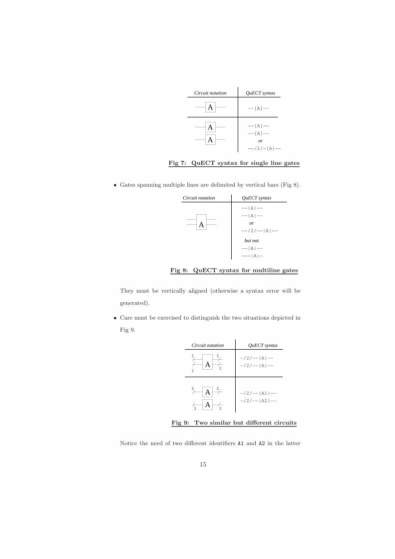
• Care must be exercised to distinguish the two situations depicted in

Fig 9.

22A

A2 2

A2

2

2

2

−/2/−−|A2|−−

−/2/−−|A1|−−

−/2/−−|A|−−

−/2/−−|A|−−


Fig 9: Two similar but different circuits

Notice the need of two different identifiers A1 and A2 in the latter

15

case. We could use any other identifiers also, as long as they are both

associated with the same gate in the classical part of the algorithm.

• Sometime we need to feed two or more nonadjacent qubits into a

gate. This often messes up the circuit diagram. Some simulators

employ a (pseudo-)gate called swap to bring the qubit lines to adja-

cent positions before feeding them into the gate. But this is easy to

achieve in QuECT as in Fig 10.

A

Apseudo−gate

Swap

or

−−−|A|−−−

−−−−−−−−−

−−−|A|−−−


Fig 10: QuECT syntax for gates spanning nonadjacent lines

Here the gate A takes the two extreme qubits as input, letting the

middle qubit “pass through”.

• Swap (pseudo-) gates are somewhat like goto-statements, and should

be generally avoided in a circuit diagram, as they reduce readability

of the diagram. A judicious layout of the lines can avoid the need

of swap gates in many situations. Also the “pass through” syntax

of QuECT as discussed above reduces the need of swapping lines.

But still there may be situations where swapping is needed. QuECT

provides the syntax shown in Fig 11 for such rare occasions.

16

−−−X−−−

−−−−−−−

−−−X−−−

−/2/−X−

−/2/−−−

−/2/−X−


Fig 11: QuECT syntax for swapping lines

The two X’s must be vertically aligned. Also each column allows

either zero or exactly 2 X’s. An attempt to swap lines with different

repeat counts generates syntax error.

• All measurements are done at the very end. A qubit to be measured

is marked with a ‘>’ at the end of the line (Fig 12).


−−/2/−−>

−−−−>

Fig 12: QuECT syntax for measurement

Next we come to the QuECT syntax for use outside the quantum

chunks. The actual quantum computation is encapsulated inside a class

called QMachine. In a real quantum computer this class will be responsi-

ble for interfacing the underlying quantum hardware. Alternatively, this

class may just run a simulator. Multiple instances of QMachine may exist

in parallel. We interact with the quantum machine at the three levels

discussed below.

17

Construction: We pass the number of qubits via its constructor.

Creating quantum gates: The quantum gates can be created in two

ways. Either they are out-of-the-box standard gates (e.g., Hadamard),

or they are classical functions in a quantum wrapper. The class

MatUnitary deals with the out-of-the-box gates. The WrapUnitary

class provides a quantum wrapper for a classical function f : {0, 1}m →

{0, 1}n. Such a function is specified by m, n and f, which are encap-

sulated inside the class Classical. Lines 6–8 of the example QuECT

code show an example with m = n = 1 and f(x) = 1 − x.

Measurements: All measurements are read back into the classical part

via the two methods getObsDist() and getObs(). The first method

returns the probability distribution as an array of length 2k where k

is the number of qubits being measured. The second method returns

an actual output. A simulator may use randomization to generate

one output from the output distribution. In an actual quantum

computer, only the second method will be available. Explicitly com-

puting the probability distribution of the measurement is a luxury

that we can afford only in a simulator.

5 Some standard algorithms

In this section we show the implementation of some well known quantum

algorithms using QuECT. The aim is not to acquaint the readers with the

details of the algorithms, rather to demonstrate different applications of

the new paradigm. Interested readers will find a very readable account of

the algorithms in [14].

18

5.1 Deutsch algorithm

The simplest possible quantum algorithm [14] is the Deutsch algorithm

which checks if a given classical “blackbox” function

f : {0, 1} → {0, 1}

is 1-1 or not.

1 QMachine qm = new QMachine(2,1);

2

3 Classical c = new Classical(1,1) {

4 public f(int x) {return 1-x;}

5 };

6 Unitary Uf = new WrapUnitary(c));

7

8 QBEGIN(qm)9 |0>--[H℄--|Uf|---[H℄-->

10 |1>--[H℄--|Uf|---------11 QEND12

13 if(qm.getObs()==1)

14 System.out.println("1-1");

15 else

16 System.out.println("not 1-1");

5.2 Deutsch Jozsa algorithm

This is a multidimensional generalization of Deutsch algorithm from the

last section [5]. Here we start with a classical “blackbox” function f :

{0, 1}n → {0, 1}, which is known to be either a constant function or

a “balanced” function , i.e., exactly half of the 2n binary n-tuples are

mapped to 0, the other half being mapped to 1.

19

The aim of the algorithm is to detect which is the case.

1 int n = 4;

2 QMachine qm = new QMachine(n+1);

3

4 Classical c = new Classical(n,1) {

5 public f(int x) {return x & 1;} //A sample balanced function

6 };


8

9 QBEGIN(qm)10 |0>--/n/--[H℄--|Uf|---[H℄-->11 |1>-------[H℄--|Uf|---------12 QEND

5.3 Simon’s periodicity algorithm

Here we are given a classical “blackbox” function f : {0, 1}n → {0, 1}n,

which is known to be periodic, i.e.,

∃b ∈ {0, 1}n such that ∀x ∈ {0, 1}nf(x ⊕ b) = f(x).

We are told that such a b exists, but we do not know what b actually is.

Simon’s algorithm [13] is a way to find this b. The algorithm starts with

some quantum computation followed by a classical linear equation solver.

We present only the quantum part here.

1 int n = 5, orthog[100];

2 QMachine qm = new QMachine(2*n);

3

4 Classical c = new Classical(n,n) {

5 public f(int x) {//f is defined here}

6 };

20


8 for(int i=0;i<100;i++) {

9 QBEGIN(qm)10 |0>--/n/--[H℄--|Uf|---[H℄-->11 |0>--/n/-------|Uf|---------12 QEND13 orthog[i]=qm.getObs();

14 }

Notice how we have put a quantum chunk inside a for-loop.

5.4 Grover’s search algorithm

Grover’s search algorithm [7] is for searching a linear list of size 2n.

1 int n = 6;

2 QMachine qm = new QMachine(n+1);

3

4 Classical c = new Classical(1,1) {

5 public f(int x) {return (x = 7? 1 : 0);} //We are searching

6 //for 7 in {0,...,63}.

7 };

8


10

11 QBEGIN(qm)12 --/n/--[H℄-13 -----------14 QEND15

16 for(int i=0;i<100;i++) {

17 QBEGIN(qm)21

18 --/n/--|Uf|--[IM℄--19 --[H℄--|Uf|--20 QEND21 }

22

23 QBEGIN(qm)24 --/n/-->25 -------26 QEND

Here we have used multiple quantum chunks. The quantum gate IM

performs an operation called inversion around mean, whose details need

not concern us here.

5.5 Shor’s algorithm and QFT

This algorithm factorizes a given integer in polynomial time [12]. Its quan-

tum part is structurally quite similar to the algorithms already discussed,

except for a Quantum Fourier Transform (QFT) block. The definition of

QFT is recursive. If we denote the n-qubit QFT gate by Qn then it is

defined recursively in terms of Qn−1. A typical step (for n = 4) is shown

in Fig 13.

Rπ/8

Rπ/4

Rπ/2

H

Q3

Fig 13: Definition of Q4 in terms of Q3

Two points set this circuit aside from the ones already discussed earlier:

recursion and the R gate which has a parameter (shown in the subscript).

We shall not go into the details of the R gate. We shall just treat it as a

blackbox and show the implementation of the circuit in QuECT.

We notice that the basic building blocks are

22

pp

m

k + m + 1

H

Rπ/2k+1

k

Fig 14:

Let us construct Qn using these. There are n recursive steps. In the

r-th step (0 ≤ r ≤ n − 1)we define Qr+1 in terms of Qr. This requires r

applications of the first block, followed by one application of the second

block. It is not difficult to see that this is achieved by the following hybrid

code.

1 for(int r=0;r<n;r++) {

2 int p = n-(r+1);

3 for(int k=1;k<r;k++) {

4 int m = r-(k+1);

5 Unitary R = new Rgate(Math.PI/(2 << k));

6 QBEGIN(qm)

7 --/p/-------

8 ------------

9 --/k/-------

10 ------[R]---

11 --/m/-------

12 QEND

13 }

14

15 int q = r-1;

16 QBEGIN(qm)

17 --/p/-------

18 -------[H]--

23

19 --/q/-------

20 QEND

21 }

Notice how we are performing both classical as well as quantum com-

putation in the same pass of a for-loop.

6 Implementation

In this section we briefly touch upon the issue of compiling a QuECT

program. As QuECT is not a programming language, but a paradigm,

it does not make strict sense to compile a QuECT program. The details

will depend on the classical host language. But certain host-independent

suggestions can be given, and this is our aim here.

Typically the compilation of any computer program proceeds in two

stages: the front end reduces the program to some abstract intermediate

representation, while the back end converts this representation to hard-

ware specific code.

For a QuECT program we suggest that the back end should produce

code in the host language with the QMachine class encapsulating all the

quantum hardware details. The following describes one approach for the

front end.

The information contained inside a single quantum chunk can be rep-

resented as follows.

1. The number of lines. Here a multi-qubit line counts as a single line.

2. A list of repeat counts, one for each line.

3. A list of Stages, where each Stage consists of a list of gates (including

swap pseudo-gates), each with its list of lines.

4. A list of lines to be measured.

An example will make this clear.

24

Suppose that we have

1 QBEGIN

2 -/n/--|A|----|Uf|---

3 --------[B]--|Uf|--->

4 ------|A|----------

5 QEND

Here we have 3 lines, the repeat counts are n, 1 and 1. There are two

stages. The first stage consists of two gates, A (spanning lines 0 and 2)

and B (spanning line 1). Measurement is done only on line 1.

It is now easy to embed this information to a suitable method in the

QMachine class, producing an ordinary Java program. The advantage of

producing the output as a high level host program is that we can borrow

the symbol table of the host language, and use the identifiers declared in

the classical part.

7 Conclusion

In this paper we have proposed a new paradigm called Quantum Embed-

ded Circuit Technique (QuECT) for programming a quantum computer.

Our approach seeks to combine the advantage of classical programming

constructs as well as the visual benefits of a quantum circuit diagram. The

paradigm can be easily implemented in any high level language, preferably

with object-oriented facilities. At present this can be used as a powerful

and versatile front end to simulators. The same approach can be easily

applied to harness the power of the real quantum computers when they

are built.

25

8 Appendix

As a proof of concept we have implemented part of the paradigm proposed

in this paper using Java as the host language. This appendix outlines

our approach. We construct a finite automaton-based lexical analyzer

that will take a QuECT program and machine translate it to a Java file.

For this purpose we employ the JLex system, which accepts a lexical

specification file, and creates a finite automaton-based lexical analyzer.

The following literate program shows a JLex specification file that achieves

our purpose. A literate program is a program written primarily for human

perusal. For the benefit of readers not accustomed to the ideosyncracies

of JLex and literate prgramming we provide a brief walk-through.

Our automaton has three states: YYINITIAL (the initial state), QUAN-

TUM and GATE.

States[1] ≡

{

// YYINITIAL is the default state, no need to declare.

%state GATE, QUANTUM

}

This macro is invoked in definition 12.

We enter the QUANTUM state on encountering the QBEGIN keyword,

and exit on the QEND keyword. Everytime we come across a quantum

gate we go into the GATE state.

The following two variables hold, respectively, the list of lines to be mea-

sured, and the list of gates encountered in the current line.

Variables[2] + ≡

{

Vector<Integer> measLst = new Vector<Integer>();

26

Vector<String> tmpList = new Vector<String>();

}

This macro is defined in definitions 2, 6, 8 and 14.


8.1 The JLex specification

Here is the main skeleton. Its important parts are elaborated upon grad-

ually. All minor technicalities are dumped in the subsection called “Mis-

cellaneous”. q.flex[3] ≡

{

Header[12]

%%

QBEGIN { baseLine = yyline+1; yybegin(QUANTUM);}

The QUANTUM state[4]

The GATE state[5]

}

This macro is attached to an output file.

The QUANTUM state[4] ≡

{

<QUANTUM> {

"[" {

count++;

if(maxCount< count) maxCount = count;

fixed=true;

yybegin(GATE);

}

27

>" "*$ {//Add a new line to be measured.

measLst.add(yyline-baseLine);

}

-+ {//Gobble up extra length of the line}

\n {/*Prepare for the next line.*/tmpList.clear();count=0;}

QEND {

Postprocess a quantum chunk[9]

}

}

}


Upon encountering a gate we first make some sanity checks, and then add

it to tmpList.

The GATE state[5] ≡

{

<GATE> {

[a-zA-Z0-9 ]+ {

curr = yytext();

if(tmpList.contains(curr)) {

System.err.println("Repeated gate in line: "+curr);

System.exit(1);

}

tmpList.add(curr);

start = yycolumn;

}

"]" {

Postprocess a gate[7]

yybegin(QUANTUM);

}

}

28

}This macro is invoked in definition 3.

8.2 Postprocessing a chunk

Variables[6] + ≡

{

Hashtable<String,Vector<Info>> s = new

Hashtable<String,Vector<Info>>();

}This macro is defined in definitions 2, 6, 8 and 14.


Postprocess a gate[7] ≡

{

Info newInfo = new Info(start,yycolumn,yyline-baseLine,count-1);

if(s.containsKey(curr)) {

System.err.println(curr+" is repeated!");

Vector<Info> v = s.get(curr);

v.add(newInfo);

}

else {

Vector<Info> tmp = new Vector<Info>();

tmp.add(newInfo);

s.put(curr,tmp);

}

}This macro is invoked in definition 5.

8.3 Postprocessing a chunk

After we finish reading a quantum chunk, we need to sum up the relevant

information in a few variables to be passed on to the quantum machine

29

qm.

Variables[8] + ≡

{

QMachine qm;

}



Postprocess a quantum chunk[9] ≡

{

Find the stages[10]

Find negMask for each stage[11]

/*The final info:

maxCount: number of stages

opList[0,...,maxCount-1]

negMask[0,...,maxCount-1]

measLst

*/

Serialize opList, negMask and measLst to tmp.q[16]

System.out.println("qm.compute(\"tmp.q\");");

yybegin(YYINITIAL);

}


Initially we have maxCount stages. For each stage we want to find its list

of gates. Each gate is identified by its name and a mask for its input lines.

Find the stages[10] ≡

30

{

/*Each gate is an Op, each stage is a list of Op’s.

We have a list of these lists.*/

Vector<Vector<Op>>

opList = new Vector<Vector<Op>>(maxCount);

for(int i=0;i<maxCount;i++)

opList.add(new Vector<Op>());

/*Pick a gate, compute its stage and mask,

add the mask to the maskList for the stage.*/

Enumeration<String> k = s.keys();

while(k.hasMoreElements()) {

String name = k.nextElement();

Vector<Info> vi = s.get(name);

System.err.println(name+":");

int max = -1;

int mask = 0;

for(Info i : vi) {

int stg = i.getStage();

mask |= (1<<i.getLine());

if(max < stg) max = stg;

}

/*Now all the info about this gate

is known: stage is max, mask is mask.

*/

31

opList.get(max).add(new Op(name,mask));

}

}


For each stage we now find a negMask (i.e., a mask for lines not affected

by the stage).

Find negMask for each stage[11] ≡

{

int negMask[] = new int[maxCount];

for(int i=0;i<maxCount;i++) {

for(Op p : opList.get(i))

negMask[i] |= p.getMask();

negMask[i] = ~negMask[i];

}

}


8.4 Miscellaneous elements

Header[12] ≡

{

Imports[13]

%%

%{

Variables[2]

%}

Miscalleneous lexer specs[15]

32

States[1]

}


Imports[13] ≡

{

import java.util.*;

import java.io.*;

}


Variables[14] + ≡

{

int maxCount=0,count = 0, start, baseLine;

String curr;

boolean fixed;

}



Miscalleneous lexer specs[15] ≡

{

%standalone

%class QuantumLexer

%column

%line

}


Serialize opList, negMask and measLst to tmp.q[16] ≡

{

try {

ObjectOutputStream oos =

new ObjectOutputStream(

33

new FileOutputStream("tmp.q"));

oos.writeObject(opList);

oos.writeObject(negMask);

oos.writeObject(measLst);

oos.flush();

oos.close();

}

catch(Exception ex) {

System.err.println("Can’t serialise!");

ex.printStackTrace();

}

}


References

[1] List of qc simulators. Available at http://www.quantiki.org/wiki/

List_of_QC_simulators. Part of a publicly editable online encyclo-

pedia on quantum computing.

[2] Lanq – a quantum imperative programming language. Available at

http://lanq.sourceforge.net/, 2007.

[3] S. Bettelli, T. Calarco, and L. Serafini. Toward and architecture

for quantum programming. CoRR. Available at http://arxiv.org/

abs/cs.PL/0103009, 2001.

[4] Andreas de Vries. jquantum—quantum computer simulator. Avail-

able at http://jquantum.sourceforge.net, 2010.

[5] D. Deutsch and R. Jozsa. Rapid solution of problems by quantum

computation. In Proceedings of the Royal Soceity of London, A, pages

439:553–558, 1992.

34

[6] S.J. Gay. Quantum programming languages: Survey and bibliogra-

phy. Bulletin of the EATCS, 86:176–196, 2005. Available at http:

//dblp.uni-trier.de.db/journals/eatcs/eatcs86.html#Gay05.

[7] L.K. Grover. Quantum mechanics helps in searching a needle in a

haystack. Physical Review Letters, 79(2):325–328, 1997.

[8] B. Omer. Quantum programming qcl. Available at http://tph.

tuwien.ac.at/oemer/doc/quprog.pdf, 2000.

[9] R. Rudiger. Quantum programming languages. The Com-

puter Journal, 50(2):134–150, 2007. Available at http://comjnl.

oxford-journals.org/cgi/content/abstract/50/2/134.

[10] P. Selinger. Towards a quantum programming language. Mathemat-

ical Structures in Computer Science, 14(4):527–586, 2004. Available

at http://www.mathstat.dal.ca/selinger/papers/qpl.pdf.

[11] S. Shary and M. Cahay. Bloch sphere simulation. Available at http:

//www.ece.uc.edu/~mcahay/blochsphere/.

[12] P.W. Shor. Polynomial-time algorithms for prime factorization and

discrete logarithms on a quantum comouter. SIAM Journal Comput-

ing, 26(5):1484–1509, 1997.

[13] D.R. Simon. On the power of quantum computation. SIAM Journal

Computing, 26(5):1474–1483, 1997.

[14] N.S. Yanofsky and M.A. Mannucci. Quantum Computing for Com-

puter Scientists. Cambridge University Press, 2008.

35

QuECT: A New Quantum Programming Paradigm - Indian Statistical

Documents

Transcript of QuECT: A New Quantum Programming Paradigm - Indian Statistical