Quantum-Statistical Geometry

Dann Passoja New York, New York

Spring 2016

2

Table of Contents INTRODUCTION 2 SCIENTIFIC AND MATHEMATICAL CONSIDERATIONS 3 THE MEASUREMENT PERSPECTIVE CLASSICAL/QUANTUM 4 PHYSICAL CHARACTERISTICS OF EQUIPMENT: 5

OBSERVABLES AND OPERATORS 5 THE GENERAL CONSISTENCY OF THE JWC 6 ENTROPY AND PROBABILITY 8 A 8 ALPHA AND THE VARIANCE 10 INSPECTION OF THE PROBABILITY TERM 12 THE RULER IS AN OBSERVABLE, A MEASURABLE OPERATOR 14 DERIVATION OF A PROBABILITY FUNCTION 14 THE METRIC PROBABILITY EQUATION 14 STATISTICS 18 STATISTICAL MECHANICS 19

MEASURING LENGTHS 19

MEASURING AREA 20 THE “KNOWN” DISTANCES 21

THE ATOMIC SCALE 24 STATES, SYSTEMS AND ASSEMBLIES 28

mω 2x2 = hω n + 12

⎛⎝⎜

⎞⎠⎟

31

THE GROUND STATE ENERGY, THE ZERO POINT ENERGY AND STRAIGHT LINES 32

Introduction

3

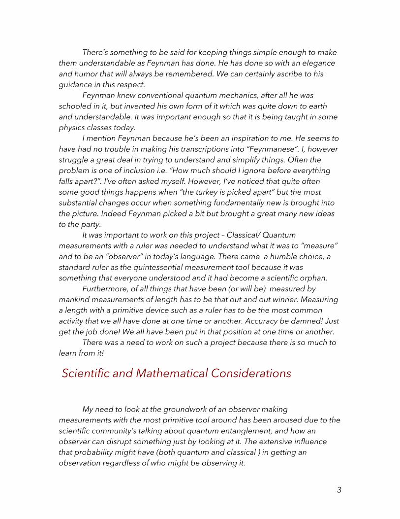
There’s something to be said for keeping things simple enough to make them understandable as Feynman has done. He has done so with an elegance and humor that will always be remembered. We can certainly ascribe to his guidance in this respect. Feynman knew conventional quantum mechanics, after all he was schooled in it, but invented his own form of it which was quite down to earth and understandable. It was important enough so that it is being taught in some physics classes today. I mention Feynman because he’s been an inspiration to me. He seems to have had no trouble in making his transcriptions into “Feynmanese”. I, however struggle a great deal in trying to understand and simplify things. Often the problem is one of inclusion i.e. “How much should I ignore before everything falls apart?”. I’ve often asked myself. However, I’ve noticed that quite often some good things happens when “the turkey is picked apart” but the most substantial changes occur when something fundamentally new is brought into the picture. Indeed Feynman picked a bit but brought a great many new ideas to the party. It was important to work on this project – Classical/ Quantum measurements with a ruler was needed to understand what it was to “measure” and to be an “observer” in today’s language. There came a humble choice, a standard ruler as the quintessential measurement tool because it was something that everyone understood and it had become a scientific orphan. Furthermore, of all things that have been (or will be) measured by mankind measurements of length has to be that out and out winner. Measuring a length with a primitive device such as a ruler has to be the most common activity that we all have done at one time or another. Accuracy be damned! Just get the job done! We all have been put in that position at one time or another. There was a need to work on such a project because there is so much to learn from it!

Scientific and Mathematical Considerations

My need to look at the groundwork of an observer making measurements with the most primitive tool around has been aroused due to the scientific community’s talking about quantum entanglement, and how an observer can disrupt something just by looking at it. The extensive influence that probability might have (both quantum and classical ) in getting an observation regardless of who might be observing it.

4

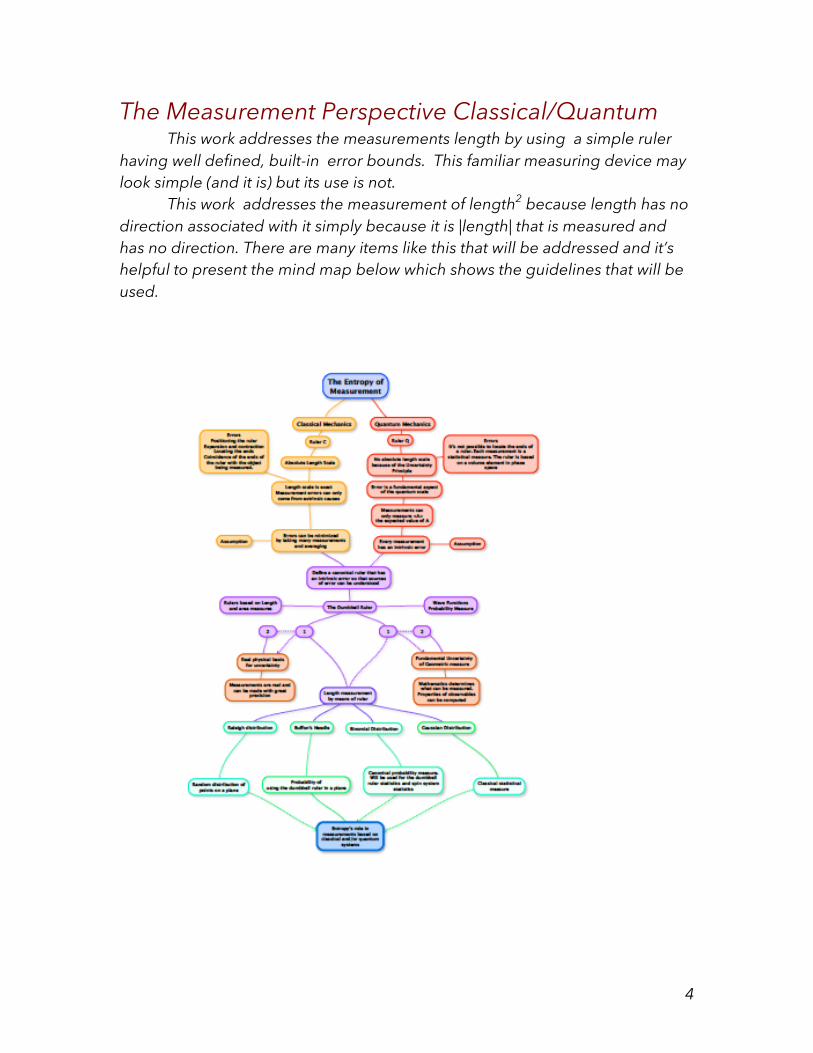
The Measurement Perspective Classical/Quantum This work addresses the measurements length by using a simple ruler having well defined, built-in error bounds. This familiar measuring device may look simple (and it is) but its use is not. This work addresses the measurement of length2 because length has no direction associated with it simply because it is |length| that is measured and has no direction. There are many items like this that will be addressed and it’s helpful to present the mind map below which shows the guidelines that will be used.

5

Figure 2 The guidelines that have been used in this work

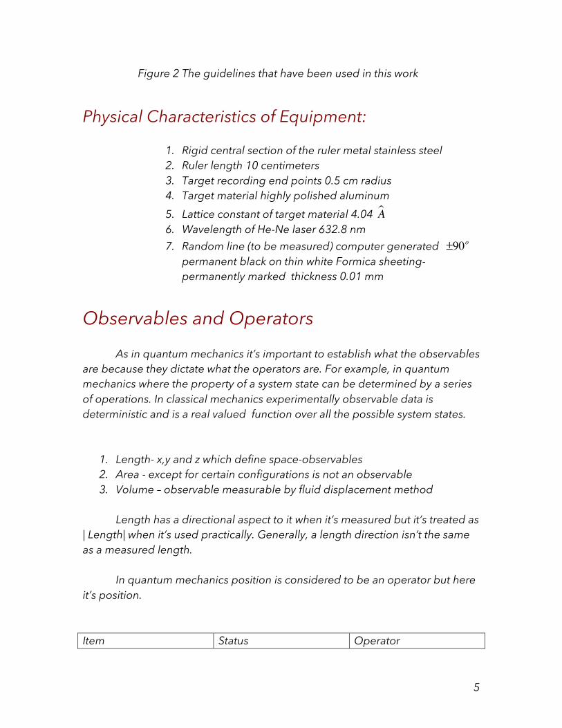
Physical Characteristics of Equipment:

1. Rigid central section of the ruler metal stainless steel 2. Ruler length 10 centimeters 3. Target recording end points 0.5 cm radius 4. Target material highly polished aluminum 5. Lattice constant of target material 4.04 A! 6. Wavelength of He-Ne laser 632.8 nm 7. Random line (to be measured) computer generated ±90o

permanent black on thin white Formica sheeting-permanently marked thickness 0.01 mm

Observables and Operators As in quantum mechanics it’s important to establish what the observables are because they dictate what the operators are. For example, in quantum mechanics where the property of a system state can be determined by a series of operations. In classical mechanics experimentally observable data is deterministic and is a real valued function over all the possible system states.

1. Length- x,y and z which define space-observables 2. Area - except for certain configurations is not an observable 3. Volume – observable measurable by fluid displacement method

Length has a directional aspect to it when it’s measured but it’s treated as | Length| when it’s used practically. Generally, a length direction isn’t the same as a measured length. In quantum mechanics position is considered to be an operator but here it’s position. Item Status Operator

6

Y (position) Observable y = −iα ∂

∂x

X (position) Observable x = iα ∂

∂x

Initially, a measurement is to be taken by a ruler that is placed in the plane of the JWC and only two points being measured. to determine a length. The measurements will show the ruler length to be an average with some variations due to small spatial variations occurring at the ruler ends as well as others that are from the curve’s natural fluctuations and more of the ruler size. The error confusion

The General Consistency of the JWC

The figures shown below illustrate some of the positions that a ruler might possess when measuring a JWC. Quite obviously in both cases show that the ruler measurement is shorter than the JWC

7

For this reason there’s an uncertainty in the measured length of line relative to the ruler. The example shows that the length of the JWC > measured length, nevertheless the ruler does measure something that is related to the wandering curve. In the second example the errors are shown to be associated with the local average defined by the rulers. The rulers measure moving averages that change and define a baseline state along the curve with fluctuations occurring around it. These are JCW fluctuations that are characteristic of the curve itself. It’s easy to see that the curve has its own fluctuations but it tends to follow the rulers that were located by a researcher in the experiment. Clearly the curve’s fluctuations show that the length of the JWC is longer than length of single rulers. It’s important to note that the ruler measures a straight line without the fine-scale end adjustments. In this respect the ruler is able to construct one type of straight line ( basically the DC level taken over a finite length spanned by the rigid part of the ruler). In fact all of the ruler movements are are a reflection of this fact. The curve is thus broken down into a series of estimates of the curve’s average taken over a fixed frequency range as dictated by the ruler’s length. So the researcher determines a different zero point average as he/she moves the ruler. There’s also an angular orientation and that’s also part of the measurement so that’s important too. There are errors associated with the measurements: the ruler measures an invariant length that’s always the same, λ , The circular regions intercept two points (in red). For every pair {they must be in pairs to define a straight line) The

8

impact points might be anywhere within the circles and will introduce errors in the measurements. These regions accommodate small ruler adjustments and must behave in this manner (introduce errors) to help ruler placement.

Entropy and Probability Let there be n measurements taken with the ruler with each one being complex or x+iy, then the total length measured ( in comparison to a sum of individual lengths2} By using the Multinomial Theorem its possible to get the coefficient (in n) for evaluating the probability and hence the entropy. That is:

x1 + x2 + x3...xk( )n = n!n1!n2 !n3!...nk !

x1n1x2

n2 ...xknk

1

k

∏

The length in these terms may be written as:

L2 = xi + iyii

k

∑⎛⎝⎜⎞⎠⎟

xi − iyii

k

∑⎛⎝⎜⎞⎠⎟= 2!n1!n2 !...nk !

xii

k

∑⎛⎝⎜⎞⎠⎟

ni

i

k

∑ iyi⎛⎝⎜

⎞⎠⎟

nn

=   2!n1!n2 !n3!...nk !

x1n1x2

n2 ...y1n1 ..

1

k

∏ −1( )n−1

. The factor involving n is concerned with the contribution of the sets that were associated with the rigid ruler. The entropy of the measurements.

Ω = 2!

nii=1

k

∏

a Measurement of a length that the ruler performs in space has a direction associated with it even though it is referred to as length. For this reason, a measured length often has to be considered as length2 . Let there be two measurements of length be made x+iy and its conjugate x-iy. Length2 x + iy( ) x − iy( ) = x2 + y2 + 2i xy − yx( ) Using the alpha-x operator and the alpha –y operator results in

9

2i xy − yx( ) = −4α

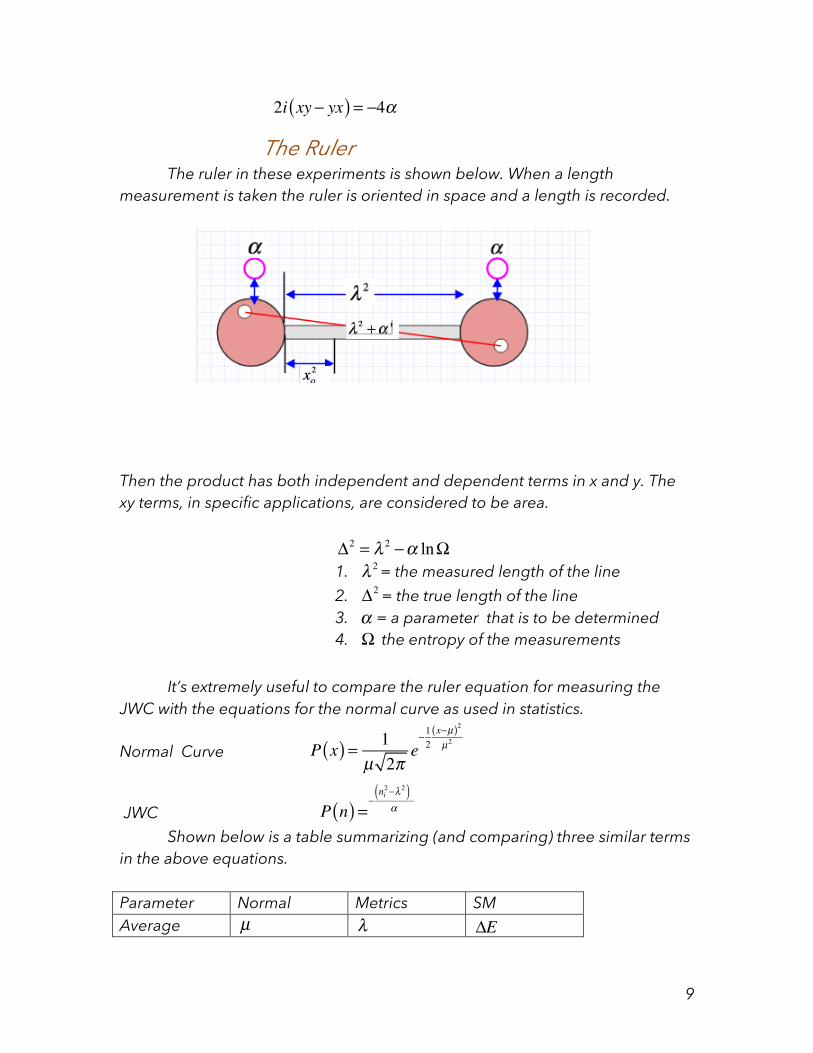
The Ruler The ruler in these experiments is shown below. When a length measurement is taken the ruler is oriented in space and a length is recorded.

Then the product has both independent and dependent terms in x and y. The xy terms, in specific applications, are considered to be area. Δ2 = λ 2 −α lnΩ

1. λ 2= the measured length of the line 2. Δ2 = the true length of the line 3. α = a parameter that is to be determined 4. Ω the entropy of the measurements

It’s extremely useful to compare the ruler equation for measuring the JWC with the equations for the normal curve as used in statistics.

Normal Curve

JWC Shown below is a table summarizing (and comparing) three similar terms in the above equations. Parameter Normal Metrics SM Average

P x( ) = 1µ 2π

e−12x−µ( )2µ2

P n( ) =−ni2−λ2( )α

µ λ ΔE

10

Variable x n n Variance T Probability Entropy 1

2ln 2πeσ 2( ) k ln W

Alpha and the Variance It appears that there might be a relationship of note between alpha and the variance in statistics. Just looking at the derivation of the ruler equation it would appear that alpha might be the area but it’s more than that. It would seem that the variance would be helpful in sorting things out

TThere are several things to keep in mind while working out these relationships:

1. There several allied variables to be aware of that are pertinent and conceptually helpful when working with alpha, namely the variance from statistics and temperature from statistical mechanics, they can act as guides.

2. The coordinates of the space to work with are imaginary, x+iy and x-iy but the data set is real one ends up with a length i.e. x2 + y2 .

3. Assumption: only part of α is related to the surface area of the error determination sites of the ruler

4. There are several other ways to handle this problem one of which is algebraic geometry, where the ruler equation would be written as a geometric product which is xy = x ⋅ y + x ∧ y but this forces the issue of the last term being an area.

First look at the spatial products I’ll form all of them just to have a complete list

• (x + iy)(x − iy) = x2 + y2 + i(xy − yx)

• x + iy( ) x − iy( ) − x2 + y2

• i(xy − yx) = i X,Y[ ] This term is known as the Commutator, squaring it results in: α = X,Y[ ] = −i Looking at the ruler equation;

σ αP x( ) P ni( ) P ε i( )

α ln P

σVar = x2 − x 2

11

The commutator has been called a cross product which is a vectored area and is the same as the last term x ∧ y in geometric algebra. This is also known as an outer product. Looking at this in matrix form:

The Commutator X,Y[ ] = x xiy −iy

⎡

⎣⎢⎢

⎤

⎦⎥⎥

α= ix −ix−y y

⎡

⎣⎢⎢

⎤

⎦⎥⎥

what is needed in the exponential term is the inverse of α then

α −1 =

i2x

12y

12x

−12y

⎡

⎣

⎢⎢⎢⎢⎢

⎤

⎦

⎥⎥⎥⎥⎥

then

Det

Δ2x

λ2y

λ2xi − Δ

2yi

⎡

⎣

⎢⎢⎢⎢⎢

⎤

⎦

⎥⎥⎥⎥⎥

=Δ2 − λ 2( )4xy

i

and this becomes the term in the exponent: So this ends up looking like a quadratic term that could be of value when it is used to calculate the different moments of metric distributions, for example the first moment of location, x is x = xP x( )dx∫ In the transform that’s been developed λ is known because it can be measured, Δ is an unknown and xy is the commutator, a vectored surface in space having an imaginary vector pointing perpendicular to it. X and Y cannot be separated in any calculations.This has all been accounted for and given by the matrix developments above. So alpha is an imaginary vectored surface defined by a

12

pair of vectors that are locked into the concept that a surface is two dimensional. So that brings alpha into focus somewhat.

Inspection of the Probability Term There are two familiar mathematical aspects that the probability density function brings to light. They both have very broad applications in other fields so perhaps it would be beneficial to bring them to light. Of course, like everything else in the world they’ll have to be carefully inspected to see where they’re applicable and where there’re not. Nevertheless, there’s always something to learn from doing that. There are two other mathematical entities that I think are relevant and useful :

• The Raleigh Distribution • The Fourier Transform

The Raleigh distribution has been around for~ 100 years and was discovered by Lord Raleigh. It’s been used to study wind speed variations, inclusion distributions in metals and many other such applications. The equation for the inclusion work is relevant since it deals with the distribution of points in space: P(r) = 2Nsre

−NSr2

It’s interesting because it’s a probability density function with an exponential to an x squared power. This should be applicable when there are quadratic terms in an energy representation such as the harmonic oscillator, where both the momentum and position terms are quadratic. The second interesting possibility of great significance comes from careful scrutiny of the probability density function (just above).

The terms in the exponent can be rearranged so that they bring about a different viewpoint. Here’s a careful review of the terms

• i the imaginary number i • Δ the “true length”, an unknown quantity • λ a length measured with a ruler-a

measurable and deterministic quantity • λ =nδ delta is cms, inches, a standard unit - a

defined, standard “metric” unit. It could also

P = e− iΔ

2−λ2

4 xy

13

be an intrinsic metric based on internal symmetry such as in a periodic solid.

• α is a vectored section of a surface that isn’t anchored in space, that is related to the nature of the measuring ruler. The recognition of the geometric product might “lock in” the true meaning and its use. It should be remembered though.

Δ2 = λ 2 +α lnP Probabilistic Ruler xy = x ⋅ y + x ∧ y Geometric Product

P(x, y) = eΔ x,y( )2−λ2

α Probability Density Function Above proof showed that alpha was imaginary, Revision of terms in the exponent

−ix2 − λ 2

α= −i

x2 − nxo( )2xy

= −i xy−nxo( )2nxoy

⎛

⎝⎜

⎞

⎠⎟

Careful scrutiny of the terms identifies the variables as being associated through the Commutator and

−ixy− xy

⎛⎝⎜

⎞⎠⎟= −i X,K[ ]

is the term in the exponent. The probability density function is related to the Commutator and the Fourier transform.

• The Fourier transform:

F k( ) = 12π

G x( )0

2π

∫ e− ikxdx

• Π k( ) = Θ x,k( )e− i X ,K[ ]

0

2π

∫ dx

is therefore directly related to the probability density function

14

The Ruler is an Observable, a Measurable Operator

Derivation of a Probability Function In the mathematics of Physics an observable is a measurable operator where the state of a system can be determined by some sequence of physical operations. What are to be expected in the errors found in the measured results? So far in this work the errors would be in a scale larger than the atomic scale.

Next, recognize a set of vectors, measure them (as usual in this work), and find

( 25

(26

The Metric Probability Equation An equation may now be forwarded for determining the probability function for making measurements. By using the alpha operator the following relationship can be found: resulting in the first equation to be studied. The right hand side of this equation is set equal to zero for the time being. The equation is in the form of the Shroedinger equation which deals with position, x and momentum p. This equation is new and it deals with the probability of measuring something in order to get an observable result. It only deals with x and y as conjugate coordinates. The equation operates in its own space and describes metrics (invariant observable forms) in a probabilistic manner. As in the Shroedinger

xxo

+ iyyo

⎛⎝⎜

⎞⎠⎟

xxo

− iyyo

⎛⎝⎜

⎞⎠⎟

xxo

+ i yyo

⎛⎝⎜

⎞⎠⎟ i

xxo

− i yyo

⎛⎝⎜

⎞⎠⎟ i= AA*

xxo

⎛⎝⎜

⎞⎠⎟

2

+ yyo

⎛⎝⎜

⎞⎠⎟

2

xxo

+ i yyo

⎛⎝⎜

⎞⎠⎟ i

xxo

+ i yyo

⎛⎝⎜

⎞⎠⎟ i= AA

AA − A*A

15

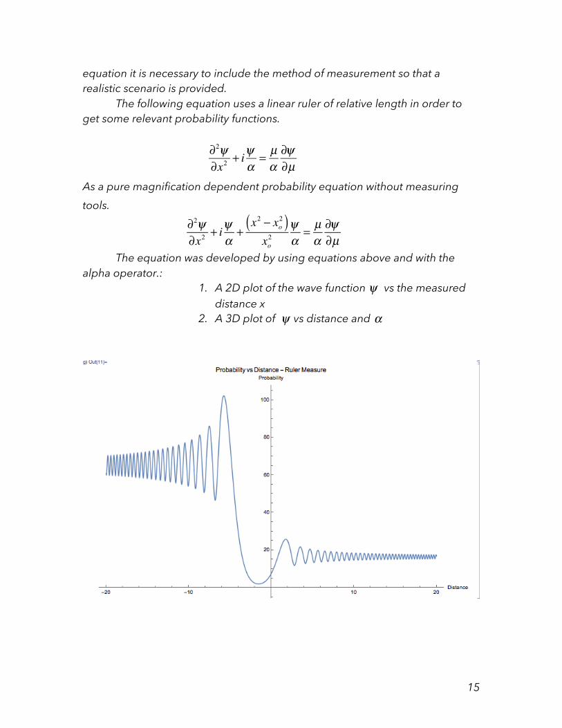
equation it is necessary to include the method of measurement so that a realistic scenario is provided. The following equation uses a linear ruler of relative length in order to get some relevant probability functions.

∂2ψ∂x2

+ iψα

= µα

∂ψ∂µ

As a pure magnification dependent probability equation without measuring tools.

∂2ψ∂x2

+ iψα

+x2 − xo

2( )xo2

ψα

= µα

∂ψ∂µ

The equation was developed by using equations above and with the alpha operator.:

1. A 2D plot of the wave function vs the measured distance x

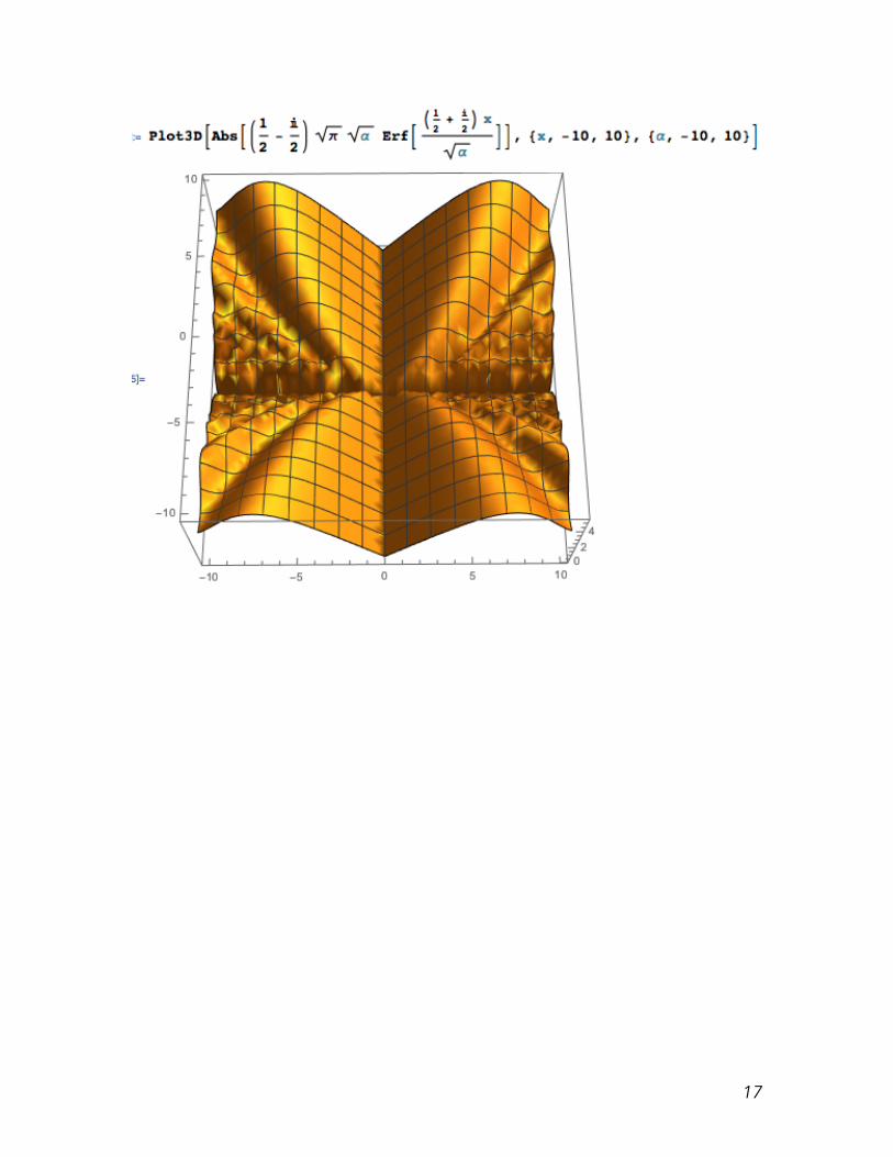
2. A 3D plot of vs distance and

ψ

ψ α

16

17

18

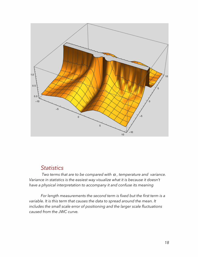
Statistics Two terms that are to be compared with α , temperature and variance. Variance in statistics is the easiest way visualize what it is because it doesn’t have a physical interpretation to accompany it and confuse its meaning For length measurements the second term is fixed but the first term is a variable. It is this term that causes the data to spread around the mean. It includes the small scale error of positioning and the larger scale fluctuations caused from the JWC curve.

19

Statistical Mechanics The term that is analogous to α is temperature which in reactions of any type acts to accelerate them. The rate of reaction depends on the ratio of energy and temperature. Temperature is analogous to the variance. Statistical mechanics and quantum mechanics have been very successful in describing the properties of assemblies of particles from those of the systems which compose them. Mechanical Properties Thermodynamic Properties Velocities momentum Temperature Position Pressure Kinetic Energy Potential Energy Entropy Specific Heat

Of the Systems Of the Assembly All the data sets N The subsets n

The Partition Function-Metric Probability The partition function of statistical mechanics is an extremely valuable tool. It helps to identify many thermodynamic quantities and to connect them with atomic states. The metric equation is similar to the partition function

Pmetrics = eΔ2−λ2

α

Pf = e−ΔG−ΔE

kT

Measuring Lengths

20

Measuring Area

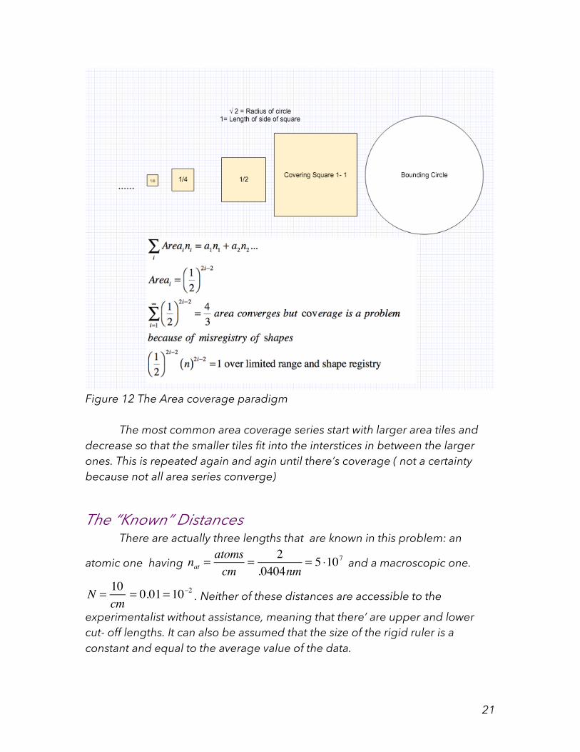
We have rulers for measuring length but we don’t have any for measuring areas this is surprising. In the case of areas measurements are taken at certain points and the area is calculated. The reason that we don’t have a ruler to measure area is shown below. There’s a circular area to be measured so a coverage strategy is used. The circle is covered with as many squares as possible and the coverage is stopped if the next squares fall outside of the circle. In order to continue a new sized smaller unit having a different shape is chosen and is fitted into the open areas… but some smaller open areas are still there so that the covering shapes must get smaller and changes shape. This could go on and never converge. It so happens that measuring area by using a ruler isn’t such a good idea, everyone knows that and that’s why we don’t have an area measuring ruler.

• In order to create a finite area having form, a series of tiles

are required .

21

Figure 12 The Area coverage paradigm The most common area coverage series start with larger area tiles and decrease so that the smaller tiles fit into the interstices in between the larger ones. This is repeated again and agin until there’s coverage ( not a certainty because not all area series converge)

The “Known” Distances There are actually three lengths that are known in this problem: an

atomic one having and a macroscopic one.

N = 10cm

= 0.01= 10−2 . Neither of these distances are accessible to the

experimentalist without assistance, meaning that there’ are upper and lower cut- off lengths. It can also be assumed that the size of the rigid ruler is a constant and equal to the average value of the data.

nat =atomscm

= 2.0404nm

= 5 ⋅107

22

Figure 13The error circles are made of a single crystal material (for convenience) having a 4 A lattice constant and a 16 A2 average area. A straight line is born i when its endpoints are activated and contact the solid parts of a ruler’s end sections. It’s possible to think of a mechanism associated with an AFM might be part of this, What’s the probability of making a force free contact? The following equation just takes probability into account.

n!N! N − n( )!

where n=1 and N=1616 cm-2 a very small probability indeed! Meaning that if there were to be registry something would need to influence n, substantially. This might be done by introducing electrical contacts as a method of registry for the line or by applying external forces

Synopsis Part I In the last sections everything was staged in the classical world and it involved true length, measured length, metrics, rulers, alpha and

23

measurements. The equation concept/equation that everything could be related to was the “Ruler Equation”

Δ2 = λ 2 +αk ln P( ) which tied probability and measurements together and introduced α which had a relationship to surfaces among other things. The probability could be related to the entropy of measurement and then to entropy in general. Its appearance in the equations and its subsequent use followed along the lines of statistical mechanics. The Gibbs free energy is G = E −TS and the Ruler Equation is:

Δ2 = λ 2 +α Ω

The statistical mechanic fundamentals of the free energy equation reveals that the terms in the equations are mostly based on quadratic functions thus their presence as the terms that support the energy in the free energy equation shouldn’t be lost when that equation is compared to the Ruler Equation. Careful scrutiny of the equation along with the use of the alpha operator led to the development of the “Measure Probability Equation”. Although similar to the Shroedinger Equation” is concerned with length instead of energy. A new type of wavefunction came forth after having gained experience with the MPE equation that was based on the “Length Commutator” Length Commutator [X,K] = i Derivations using the Ruler Equation showed that the Length Commutator was related to the probability:

• Step 1 η = e− i X ,K[ ] this step in the derivation indicated that the Length commutator was present in an exponential term

• Step 2 0

∞

∫ P x,k( )0

∞

∫ dxdk = 1

• Step 3 The Commutator was a matrix

24

• Step 4 The entire transformation, probability and all was a Fourier transform using the commutator as a matrix in an

integral thus φ k[ ] = P x,k( )e− i x,k[ ]

−∞

∞

∫ dx

The Atomic Scale

Measure on the Atomic Scale uses Momentum, Position, Uncertainty and Probability To transfer knowledge and understanding from the classic world to the quantum world is difficult for many reasons. What seemed to be a tried and true laws in Classical Physics, ones that would make predictions that led to rational and understandable consequences didn’t stand up under the scrutiny of the Quantum magnifying glass. Things such as electrons were both particles and waves - the classicists felt that the quantum people never could understand the meaning of gender either. In the case of this paper our transition goes from the macroscopic to the atomic world having several things in our favor. There are several very powerful rules and laws that are operable in the atomic world and so we’re going to accept them and use them to our benefit, rather than remain in quandary about their purpose and use. Furthermore, the atomic world is one of position, momentum, spin, magnetic moments, electrons that are invisible to the eye and nuclei that are relatively heavy but occupy surprisingly little space-so little, in fact, that their bulk is hardly noticed at the energies that are important to us.

25

Energy, the Ruler of the Atomic Scale On any scale energy RULES! So lets write something that’s important about it here’s what’s known as thee Hamiltonian: It says that everything that we know about follows this equation which says (in words) All Energy is composed of two parts Kinetic Energy and Potential Energy

This is the kinetic energy operator note that it’s quadratic in momentum

both quadratic variables

V (x,t) = 12mω 2x2 -Potential Energy Harmonic Oscillator

Here’s the first important thing to notice This a window into the non-relativistic atomic world, the Shroedinger Equation for the harmonic oscillator.. It’s very much like Hamilton’s equation but it’s more complicated and interesting:

− !

2

2m∂2ψ r,t( )

∂r2+ 12mωr2ψ r,t( ) = i! ∂ψ r,t( )

∂t

Here’s the second most important thing to notice It was Paul Dirac a famous scientist from Cambridge, England who introduced this elegant trick: you can make things easy on yourself if you want to work with the harmonic oscillator if you do this and call this the Creation and Annihilation Expansion -or for short the C/A Operators.

26

xxo

+ i ppo

⎛⎝⎜

⎞⎠⎟

xxo

− i ppo

⎛⎝⎜

⎞⎠⎟

=

xxo

⎛⎝⎜

⎞⎠⎟

2

+ ppo

⎛⎝⎜

⎞⎠⎟

2

− i xp − pxxo po

⎛⎝⎜

⎞⎠⎟

and if any of these terms should unexpectedly → 0 or → ∞ change formats ie. matrix form will keep them alive. For example the term below will not survive a binomial expansion-

−i xp − pxh

⎛⎝⎜

⎞⎠⎟ =

1h

x x−ip ip

⎡

⎣⎢⎢

⎤

⎦⎥⎥

I don’t mean to repeat this but it’s important to do this because of a number of things that are to follow.

xxo

+ i ppo

⎛⎝⎜

⎞⎠⎟

xxo

− i ppo

⎛⎝⎜

⎞⎠⎟

= xxo

⎛⎝⎜

⎞⎠⎟

2

+ ppo

⎛⎝⎜

⎞⎠⎟

2

+ 1h

x x−ip ip

⎡

⎣⎢⎢

⎤

⎦⎥⎥

Det

xxo

i ppo

i ppo

xxo

⎡

⎣

⎢⎢⎢⎢⎢

⎤

⎦

⎥⎥⎥⎥⎥

= xxo

⎛⎝⎜

⎞⎠⎟

2

+ ppo

⎛⎝⎜

⎞⎠⎟

2

Det

xxo

xxo

−i ppo

i ppo

⎡

⎣

⎢⎢⎢⎢⎢

⎤

⎦

⎥⎥⎥⎥⎥

= 2i xph

This means that it’s possible to keep all the terms in the equations by switching to a matrix format. I’ll use the General Form of the Ruler Equation to start appreciating that we need some sort of a ruler to measure things on the atomic scale – say from the Bohr radius 0.529 A and upward and ~ 13.6 eV. The details contained in the numbers won’t matter until later when we’ll need them in order to find our mistakes. A More Detailed Ruler Equation is: Δ2 =λ 2+α Ω or, keeping W for the representation of probability Δ2 = λ 2 +α log W Δ2 = the true length that exists between any two points that define a straight line. No wiggles allowed, no matter, no energy this straight line can’t be real because of that it’s a theoretical construction that fulfills every purpose of Δ2

27

λ 2=the measured length of a curve done with straight line segments that supported by metrics- distances that are known and used repeatedly-basically a quantum of length. α a physical-statistical entity that is related to a surface because it’s a surface having an imaginary vector pointing out of it , but alpha is very much like Planck’s constant in that it’s just not entirely a “Thing”. Three different simple mathematical things were factored and emerged in the C/A development (1 x2 terms 2) y2 and 3) xy terms . Starting with a simple premise- this is some form of geometry again, it’s relatively straightforward to consider 1 and 2 to be the magnitudes of line segments and 3 to be some sort of a surface term. So a potential atomic ruler equation might be:

ppo

⎛⎝⎜

⎞⎠⎟

2

= xxo

⎛⎝⎜

⎞⎠⎟

2

+ 2ix, p[ ]h

logW

W = e− ih

ppo

⎛⎝⎜

⎞⎠⎟

2

− xxo

⎛⎝⎜

⎞⎠⎟

2

2 x,p[ ]

x, p[ ] = Detxxo

xxo

−i ppo

i ppo

⎡

⎣

⎢⎢⎢⎢⎢

⎤

⎦

⎥⎥⎥⎥⎥

28

States, Systems and Assemblies

The above figure shows several fundamental concepts that might be associated with the existence of a straight line on the atomic scale. A straight line is, in fact, a theoretical idea. When considered in terms of an atomic structure there are accommodations to be made. There must be a clear separation, theoretically, at least, , between a straight line (an idea coming from the Geometers of Grecian times), energy that might be associated with a straight line and matter that might represent a straight line having form and substance.

1. In a periodic solid, since a line has no directional constraints and,where its periodic intercepts can vary ie 1,2,3… -> then perhaps 4,8,12,16…are where a straight line might be “anchored”

2. It’s possible to conceive of a straight line entering an atom and getting trapped . The line has no physical

29

existence so once inside the atom it might get longer or shorter (according to the Uncertainty Principle) . In this case there’s entropy associated with a trapped line. Therefore there’s a need to estimate its length but there’s no way to do it. There doesn’t seem to be any way around this conundrum without bringing in quantum mechanics. Dressing up the line so that it’s possible to speak of the line’s energy makes some sort of identification possible even though it would be blurry and difficult to locate.

3. In certain instances the line may just disappear somewhere and become associated with an entire atomic structure. Or it could blink on and off.

Shown below is another scenario, showing that it might it's possible to think about straight line segments that are connected to some atoms. It’s then possible to conceive of a mathematical function defined on them (barely!– a derivative for example) with atoms perturbing and, perhaps, offering a support for the segments. The idea here is to begin to think about how discreteness and fields might perturb a perfectly well defined mathematical idea such as a derivative.

30

A Ruler Measuring the Width of a Box Shown below is a simple model of a ruler measuring the width of a box. When the ruler is too long it overlaps the ends of the box and isn’t able to perform a measurement, on the other hand, if it’s too short it just falls to the bottom and can’t perform a measurement. In either case the ruler is not connected to its environment (the box). When the ruler just is able to measure the width of the box, it’s assumed that it can share energy with the box. This therefore is a “ruler in a box” problem along with its boundary values.

E = h2n2

2mL2

L = hmω

n n=1,2,3,...

in which case it’s simple to show that this can be a ruler having hmω

metrics

being registered at n= 1, 2, 3, … The value of the metric for silicon is 0.0403A.

31

In keeping with the boundary conditions, this model can also be used in the case of the harmonic oscillator. When the ruler just fits it becomes coupled to the walls where the {classical) vibrational elastic waves have energy mω 2x2 the ruler transfers this energy but it’s quantized and therefore

mω 2x2 = hω n + 12

⎛⎝⎜

⎞⎠⎟

…

The ruler now is quantized n=1,2,3 the important ground state energy is included in these values also. That’s next on the list.

x = hmω

n + 12

⎛⎝⎜

⎞⎠⎟

32

The Ground State Energy, The Zero Point Energy and Straight Lines

33