Tutorial on Schubert Varieties and Schubert Calculus - icerm
JOURNAL OF THEAMERICAN MATHEMATICAL SOCIETYVolume 10, Number 3, July 1997, Pages 565–596S 0894-0347(97)00237-3
QUANTUM SCHUBERT POLYNOMIALS
SERGEY FOMIN, SERGEI GELFAND, AND ALEXANDER POSTNIKOV
In this paper, we compute Gromov-Witten invariants of the flag manifold using anew combinatorial construction for its quantum cohomology ring. Our constructionprovides quantum analogues of the Bernstein-Gelfand-Gelfand results on the coho-mology of the flag manifold, and the Lascoux-Schutzenberger theory of Schubertpolynomials. We also derive the quantum Monk’s formula.
1. Introduction
Let Fln be the manifold of complete flags in the n-dimensional linear space Cn.The cohomology ring H∗(Fln ,Z) can be described in two different ways. An al-gebraic description due to A. Borel [5] represents it canonically as a quotient of apolynomial ring:
H∗(Fln ,Z) ∼= Z[x1, . . . , xn]/In ,(1.1)
where In is the ideal generated by symmetric polynomials in x1, . . . , xn withoutconstant term.
Another, geometric, description of the cohomology ring of the flag manifold isbased on the decomposition of Fln into Schubert cells. These are even-dimensionalcells indexed by the elements w of the symmetric group Sn . The corresponding co-homology classes σw , called Schubert classes, form an additive basis in H∗(Fln ,Z).
To relate the two descriptions, one would like to determine which elements ofZ[x1, . . . , xn]/In correspond to the Schubert classes under the isomorphism (1.1).This was first done in [2] (see also [8]) for a general case of an arbitrary complexsemisimple Lie group. Later, Lascoux and Schutzenberger [22] came up with acombinatorial version of this theory (for the type A) by introducing remarkablepolynomial representatives of the Schubert classes σw called Schubert polynomialsand denoted Sw .
Recently, motivated by ideas that came from the string theory [31, 30], math-ematicians defined, for any Kahler algebraic manifold X , the (small) quantum co-homology ring QH∗(X,Z), which is a certain deformation of the classical cohomol-ogy ring (see, e.g., [28, 19, 14] and references therein). The additive structure ofQH∗(X ,Z) is essentially the same as that of ordinary cohomology. In particular,QH∗(Fln ,Z) is canonically isomorphic, as an abelian group, to the tensor prod-uct H∗(Fln ,Z) ⊗ Z[q1, . . . , qn−1], where the qi are formal variables (deformationparameters). The multiplicative structure of the quantum cohomology is however
Received by the editors July 8, 1996 and, in revised form, December 23, 1996.1991 Mathematics Subject Classification. Primary 14M15; Secondary 05E15, 14N10.Key words and phrases. Gromov-Witten invariants, quantum cohomology, flag manifold, Schu-
bert polynomials.The first author was supported in part by NSF grant DMS-9400914.
c©1997 American Mathematical Society
565
566 SERGEY FOMIN, SERGEI GELFAND, AND ALEXANDER POSTNIKOV
deformed compared to the classical cohomology ring H∗(Fln ,Z), and specializesto it in the classical limit q1 = · · · = qn−1 = 0. The structure constants for thequantum multiplication are the 3-point Gromov-Witten invariants of genus 0. In-formally, these invariants count equivalence classes of certain rational curves in thealgebraic variety Fln .
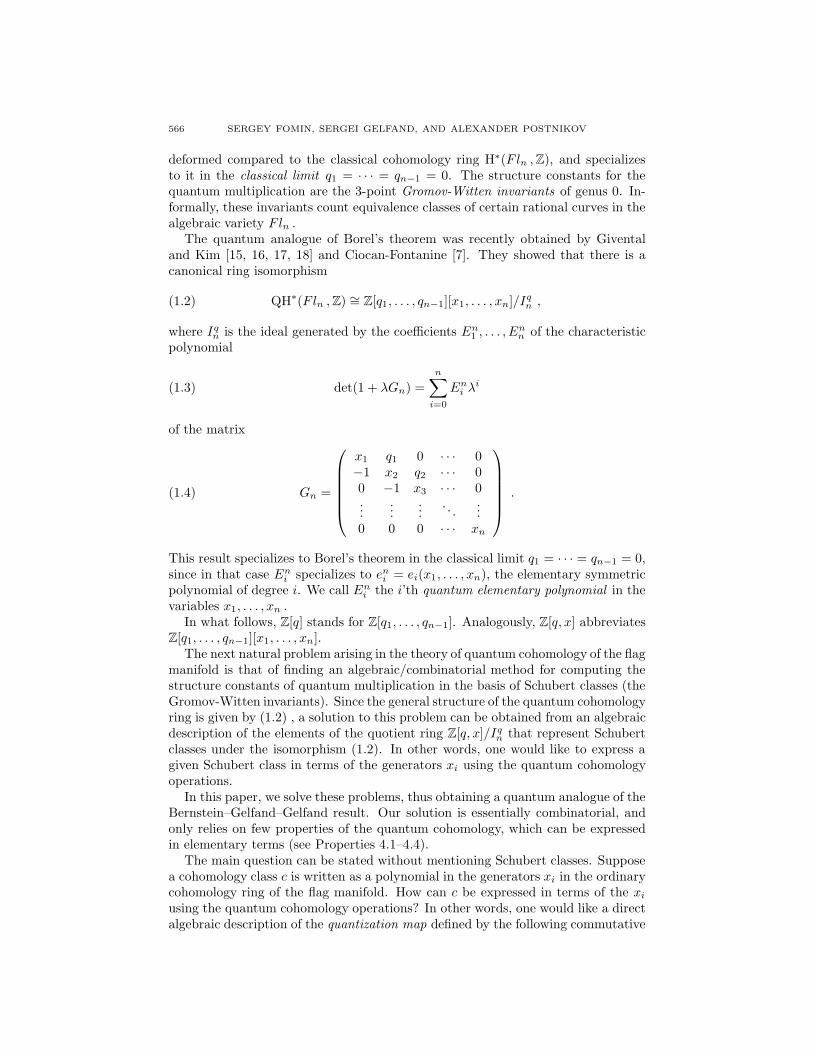
The quantum analogue of Borel’s theorem was recently obtained by Giventaland Kim [15, 16, 17, 18] and Ciocan-Fontanine [7]. They showed that there is acanonical ring isomorphism
QH∗(Fln ,Z) ∼= Z[q1, . . . , qn−1][x1, . . . , xn]/Iqn ,(1.2)
where Iqn is the ideal generated by the coefficients En1 , . . . , E
nn of the characteristic
polynomial
det(1 + λGn) =
n∑i=0
Eni λ
i(1.3)
of the matrix
Gn =
x1 q1 0 · · · 0−1 x2 q2 · · · 00 −1 x3 · · · 0...
......
. . ....
0 0 0 · · · xn
.(1.4)
This result specializes to Borel’s theorem in the classical limit q1 = · · · = qn−1 = 0,since in that case En
i specializes to eni = ei(x1, . . . , xn), the elementary symmetricpolynomial of degree i. We call En
i the i’th quantum elementary polynomial in thevariables x1, . . . , xn .
In what follows, Z[q] stands for Z[q1, . . . , qn−1]. Analogously, Z[q, x] abbreviatesZ[q1, . . . , qn−1][x1, . . . , xn].
The next natural problem arising in the theory of quantum cohomology of the flagmanifold is that of finding an algebraic/combinatorial method for computing thestructure constants of quantum multiplication in the basis of Schubert classes (theGromov-Witten invariants). Since the general structure of the quantum cohomologyring is given by (1.2) , a solution to this problem can be obtained from an algebraicdescription of the elements of the quotient ring Z[q, x]/Iqn that represent Schubertclasses under the isomorphism (1.2). In other words, one would like to express agiven Schubert class in terms of the generators xi using the quantum cohomologyoperations.
In this paper, we solve these problems, thus obtaining a quantum analogue of theBernstein–Gelfand–Gelfand result. Our solution is essentially combinatorial, andonly relies on few properties of the quantum cohomology, which can be expressedin elementary terms (see Properties 4.1–4.4).
The main question can be stated without mentioning Schubert classes. Supposea cohomology class c is written as a polynomial in the generators xi in the ordinarycohomology ring of the flag manifold. How can c be expressed in terms of the xiusing the quantum cohomology operations? In other words, one would like a directalgebraic description of the quantization map defined by the following commutative
QUANTUM SCHUBERT POLYNOMIALS 567
diagram:
H∗(Fln)⊗ Z[q] ∼= Z[q, x]/In
↓ ↓quantization map
QH∗(Fln) ∼= Z[q, x]/Iqn
(1.5)
In this diagram, the horizontal maps correspond to the ring isomorphisms (1.1) and(1.2); the left vertical arrow represents the tautological Z[q]-linear map.
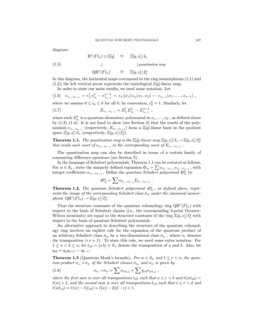
In order to state our main results, we need some notation. Let
ei1...in−1 = e1i1e2i2 · · · en−1
in−1= ei1(x1) ei2(x1 , x2) · · · ein−1(x1 , . . . , xn−1) ,(1.6)
where we assume 0 ≤ ik ≤ k for all k; by convention, ek0 = 1. Similarly, let
Ei1...in−1 = E1i1E
2i2 · · ·En−1
in−1,(1.7)
where each Ekik
is a quantum elementary polynomial in x1, . . . , xk , as defined aboveby (1.3)–(1.4). It is not hard to show (see Section 3) that the cosets of the poly-nomials ei1...in−1 (respectively, Ei1...in−1) form a Z[q]-linear basis in the quotientspace Z[q, x]/In (respectively, Z[q, x]/Iqn).
Theorem 1.1. The quantization map is the Z[q]-linear map Z[q, x]/In→Z[q, x]/Iqnthat sends each coset of ei1...in−1 to the corresponding coset of Ei1...in−1 .
The quantization map can also be described in terms of a certain family ofcommuting difference operators (see Section 5).
In the language of Schubert polynomials, Theorem 1.1 can be restated as follows.For w ∈ Sn , write the uniquely defined expansion Sw =
∑αi1...in−1ei1...in−1 , with
integer coefficients αi1...in−1 . Define the quantum Schubert polynomial Sqw by
Sqw =
∑αi1...in−1Ei1...in−1 .
Theorem 1.2. The quantum Schubert polynomial Sqw , as defined above, repre-
sents the image of the corresponding Schubert class σw under the canonical isomor-phism QH∗(Fln) → Z[q, x]/Iqn .
Thus the structure constants of the quantum cohomology ring QH∗(Fln) withrespect to the basis of Schubert classes (i.e., the corresponding 3-point Gromov-Witten invariants) are equal to the structure constants of the ring Z[q, x]/Iqn withrespect to the basis of quantum Schubert polynomials.
An alternative approach to describing the structure of the quantum cohomol-ogy ring involves an explicit rule for the expansion of the quantum product ofan arbitrary Schubert class σw by a two-dimensional class σsr , where sr denotesthe transposition (r r + 1). To state this rule, we need some extra notation. For1 ≤ a < b ≤ n, let tab = (a b) ∈ Sn denote the transposition of a and b. Also, letqab = qaqa+1 · · · qb−1 .
Theorem 1.3 (Quantum Monk’s formula). For w ∈ Sn and 1 ≤ r < n, the quan-tum product σsr ∗ σw of the Schubert classes σsr and σw is given by
σsr ∗ σw =∑
σwtab +∑
qcdσwtcd ,(1.8)
where the first sum is over all transpositions tab such that a ≤ r < b and `(wtab) =`(w) + 1, and the second sum is over all transpositions tcd such that c ≤ r < d and`(wtcd) = `(w) − `(tcd) = `(w)− 2(d− c) + 1.

568 SERGEY FOMIN, SERGEI GELFAND, AND ALEXANDER POSTNIKOV
In the classical limit q1 = · · · = qn−1 = 0, equation (1.8) becomes the classicalMonk’s formula [26] (see Theorem 2.8).
We present below the general outline of the paper. In Section 2, the necessarybackground is reviewed, including basic facts from the theory of classical cohomol-ogy of the flag manifolds, ordinary Schubert polynomials, quantum cohomology,and Gromov-Witten invariants. In Section 3, we study the polynomials ei1...im andtheir quantum counterparts Ei1...im . This allows us to derive some basic propertiesof the combinatorially defined quantum Schubert polynomials Sq
w , and describe amethod for their computation. Section 4 is devoted to the proof of Theorem 1.2.The crucial ingredient of this proof is the orthogonality property, whose combina-torial proof is postponed until Section 6. This proof relies on a description of thequantization map that involves a family of commuting difference operators, whichis given in Section 5. Section 7 contains the proof of the quantum Monk’s for-mula. In Section 8, we review our main results. Following that, we discuss inSection 9 the problem of axiomatic characterization of the quantum Schubert poly-nomials. Our particular choice of polynomial representatives of Schubert classes isuniquely determined by the stability property discussed in Section 10. The quan-tum complete homogeneous polynomials are studied in Section 11. In Section 12,we apply Grobner basis techniques for efficient computation of k-point Gromov-Witten invariants of the flag manifolds. Sections 13 and 14 contain the tables ofGromov-Witten invariants for the flag manifolds Fl3 and Fl4 , and the tables ofquantum Schubert polynomials for S2 , S3 , and S4 .
Among the many open problems in the field, we will only mention a few. Thefirst natural task is to extend the theory to the case of an arbitrary root system,thus providing a quantum analogue to the corresponding result in [2]. It would beinteresting to find a combinatorial construction for the quantum Schubert polyno-mials for other classical series (cf. [4, 11, 27]), and to compute the Gromov-Witteninvariants of partial flag manifolds1 (cf. [1, 16]).
2. Preliminaries
2.1. Flag manifold. We begin with reviewing the basic results on the classicalcohomology of the flag manifold. Details can be found, e.g., in [13, Chapter 10].
Let Fln be the flag manifold whose points are the complete flags of subspaces
U. = (U1 ⊂ U2 ⊂ · · · ⊂ Un = Cn) , dimUi = i ,(2.1)
in the n-dimensional linear space Cn. The space Fln comes equipped with the flagof tautological vector bundles 0 = E0 ⊂ E1 ⊂ · · · ⊂ En−1 ⊂ En = Cn ; the fiber ofEi at the point (2.1) is Ui .
Consider the ring homomorphism
π : Z[x1, . . . , xn] −→ H∗(Fln ,Z)(2.2)
given by π(xi) = −c1(Ei/Ei−1), where c1(Ei/Ei−1) ∈ H2(Fln ,Z), i = 1, . . . , n, isthe first Chern class of the line bundle Ei/Ei−1 . Let In ⊂ Z[x1, . . . , xn] be the idealgenerated by all symmetric polynomials without constant term—or, equivalently,by the elementary symmetric polynomials ei(x1, . . . , xn), for i = 1, . . . , n. Thefollowing classical result is due to A. Borel [5].
1Note added in proof. The latest developments in “quantum Schubert calculus” are reviewedand unified in W. Fulton’s recent note “Universal Schubert polynomials”.
QUANTUM SCHUBERT POLYNOMIALS 569
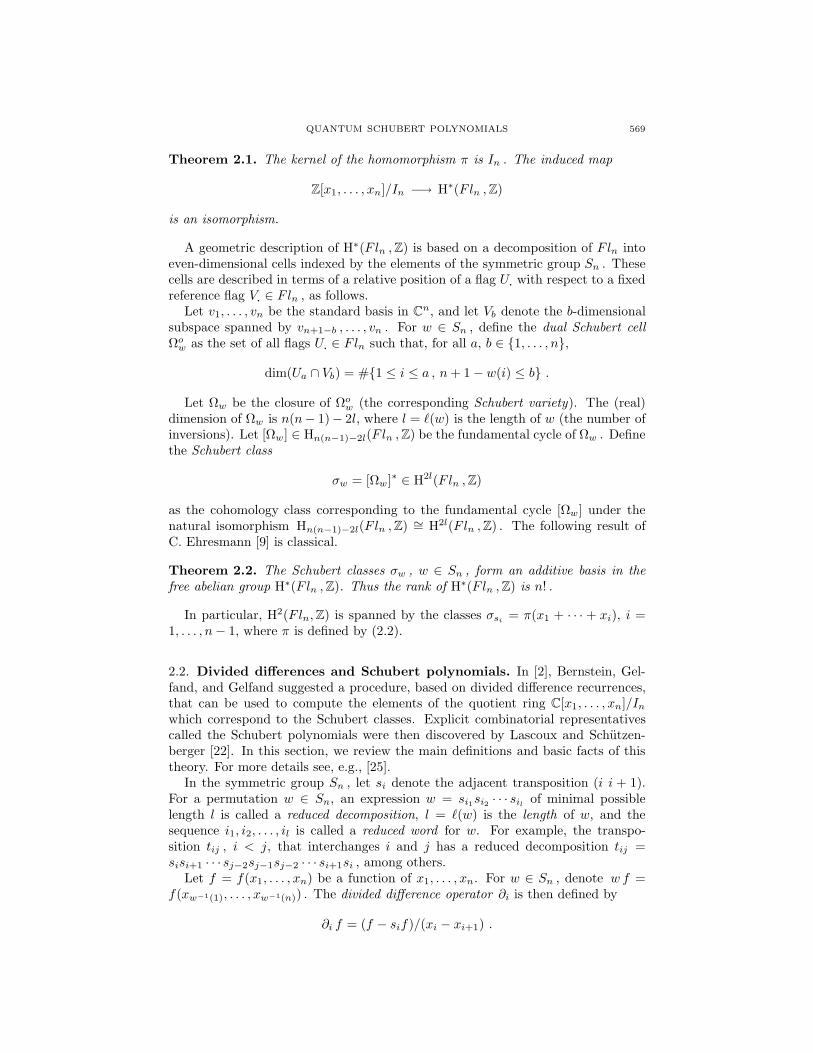
Theorem 2.1. The kernel of the homomorphism π is In . The induced map
Z[x1, . . . , xn]/In −→ H∗(Fln ,Z)
is an isomorphism.
A geometric description of H∗(Fln ,Z) is based on a decomposition of Fln intoeven-dimensional cells indexed by the elements of the symmetric group Sn . Thesecells are described in terms of a relative position of a flag U. with respect to a fixedreference flag V. ∈ Fln , as follows.
Let v1, . . . , vn be the standard basis in Cn, and let Vb denote the b-dimensionalsubspace spanned by vn+1−b , . . . , vn . For w ∈ Sn , define the dual Schubert cellΩow as the set of all flags U. ∈ Fln such that, for all a, b ∈ 1, . . . , n,
dim(Ua ∩ Vb) = #1 ≤ i ≤ a , n+ 1− w(i) ≤ b .
Let Ωw be the closure of Ωow (the corresponding Schubert variety). The (real)
dimension of Ωw is n(n− 1)− 2l, where l = `(w) is the length of w (the number ofinversions). Let [Ωw] ∈ Hn(n−1)−2l(Fln ,Z) be the fundamental cycle of Ωw . Definethe Schubert class
σw = [Ωw]∗ ∈ H2l(Fln ,Z)
as the cohomology class corresponding to the fundamental cycle [Ωw] under thenatural isomorphism Hn(n−1)−2l(Fln ,Z) ∼= H2l(Fln ,Z) . The following result ofC. Ehresmann [9] is classical.
Theorem 2.2. The Schubert classes σw , w ∈ Sn , form an additive basis in thefree abelian group H∗(Fln ,Z). Thus the rank of H∗(Fln ,Z) is n! .
In particular, H2(Fln,Z) is spanned by the classes σsi = π(x1 + · · · + xi), i =1, . . . , n− 1, where π is defined by (2.2).
2.2. Divided differences and Schubert polynomials. In [2], Bernstein, Gel-fand, and Gelfand suggested a procedure, based on divided difference recurrences,that can be used to compute the elements of the quotient ring C[x1, . . . , xn]/Inwhich correspond to the Schubert classes. Explicit combinatorial representativescalled the Schubert polynomials were then discovered by Lascoux and Schutzen-berger [22]. In this section, we review the main definitions and basic facts of thistheory. For more details see, e.g., [25].
In the symmetric group Sn , let si denote the adjacent transposition (i i + 1).For a permutation w ∈ Sn, an expression w = si1si2 · · · sil of minimal possiblelength l is called a reduced decomposition, l = `(w) is the length of w, and thesequence i1, i2, . . . , il is called a reduced word for w. For example, the transpo-sition tij , i < j, that interchanges i and j has a reduced decomposition tij =sisi+1 · · · sj−2sj−1sj−2 · · · si+1si , among others.
Let f = f(x1, . . . , xn) be a function of x1, . . . , xn. For w ∈ Sn , denote w f =f(xw−1(1), . . . , xw−1(n)) . The divided difference operator ∂i is then defined by
∂i f = (f − sif)/(xi − xi+1) .
570 SERGEY FOMIN, SERGEI GELFAND, AND ALEXANDER POSTNIKOV
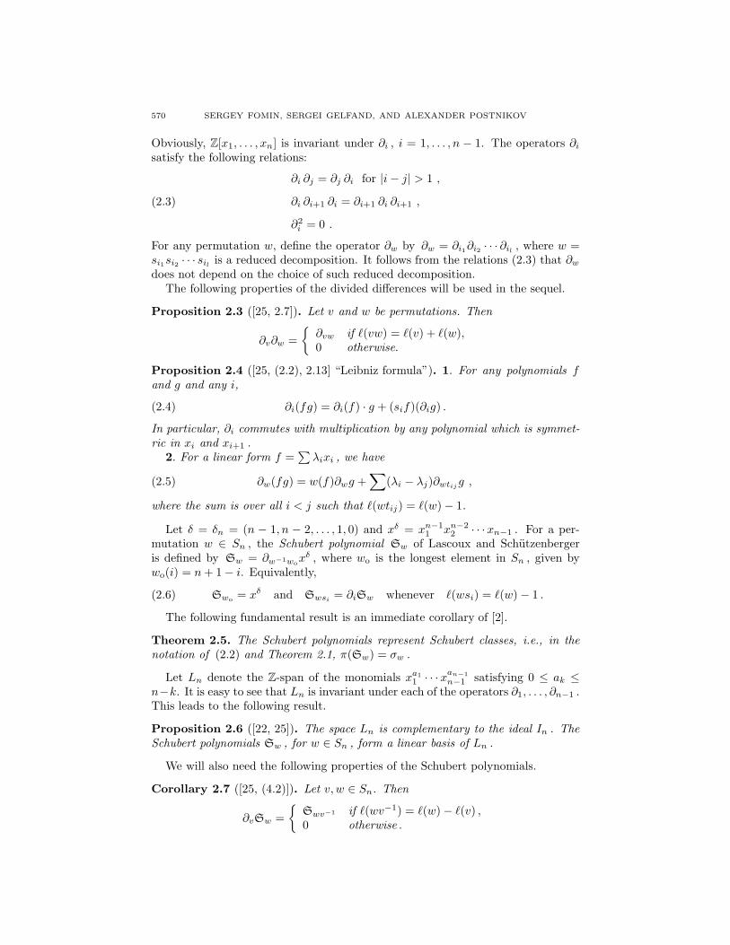
Obviously, Z[x1, . . . , xn] is invariant under ∂i , i = 1, . . . , n − 1. The operators ∂isatisfy the following relations:
∂i ∂j = ∂j ∂i for |i− j| > 1 ,
∂i ∂i+1 ∂i = ∂i+1 ∂i ∂i+1 ,
∂2i = 0 .
(2.3)
For any permutation w, define the operator ∂w by ∂w = ∂i1∂i2 · · · ∂il , where w =si1si2 · · · sil is a reduced decomposition. It follows from the relations (2.3) that ∂wdoes not depend on the choice of such reduced decomposition.
The following properties of the divided differences will be used in the sequel.
Proposition 2.3 ([25, 2.7]). Let v and w be permutations. Then
∂v∂w =
∂vw if `(vw) = `(v) + `(w),0 otherwise.
Proposition 2.4 ([25, (2.2), 2.13] “Leibniz formula”). 1. For any polynomials fand g and any i,
∂i(fg) = ∂i(f) · g + (sif)(∂ig) .(2.4)
In particular, ∂i commutes with multiplication by any polynomial which is symmet-ric in xi and xi+1 .
2. For a linear form f =∑λixi , we have
∂w(fg) = w(f)∂wg +∑
(λi − λj)∂wtijg ,(2.5)
where the sum is over all i < j such that `(wtij) = `(w)− 1.
Let δ = δn = (n − 1, n − 2, . . . , 1, 0) and xδ = xn−11 xn−2
2 · · ·xn−1 . For a per-mutation w ∈ Sn , the Schubert polynomial Sw of Lascoux and Schutzenbergeris defined by Sw = ∂w−1wo
xδ , where wo is the longest element in Sn , given bywo(i) = n+ 1− i. Equivalently,
Swo = xδ and Swsi = ∂iSw whenever `(wsi) = `(w)− 1 .(2.6)
The following fundamental result is an immediate corollary of [2].
Theorem 2.5. The Schubert polynomials represent Schubert classes, i.e., in thenotation of (2.2) and Theorem 2.1, π(Sw) = σw .
Let Ln denote the Z-span of the monomials xa11 · · ·xan−1
n−1 satisfying 0 ≤ ak ≤n−k. It is easy to see that Ln is invariant under each of the operators ∂1, . . . , ∂n−1 .This leads to the following result.
Proposition 2.6 ([22, 25]). The space Ln is complementary to the ideal In . TheSchubert polynomials Sw , for w ∈ Sn , form a linear basis of Ln .
We will also need the following properties of the Schubert polynomials.
Corollary 2.7 ([25, (4.2)]). Let v, w ∈ Sn. Then
∂vSw =
Swv−1 if `(wv−1) = `(w)− `(v) ,0 otherwise .
QUANTUM SCHUBERT POLYNOMIALS 571
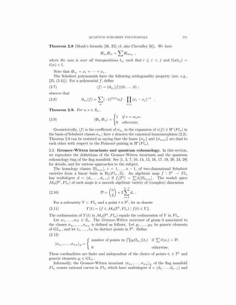
Theorem 2.8 (Monk’s formula [26, 25]; cf. also Chevalley [6]). We have
SsrSw =∑
Swtij ,
where the sum is over all transpositions tij such that i ≤ r < j and `(wtij) =`(w) + 1.
Note that Ssr = x1 + · · ·+ xr .The Schubert polynomials have the following orthogonality property (see, e.g.,
[25, (5.4)]). For a polynomial f , define
〈f〉 = (∂wo(f))(0, . . . , 0) ;(2.7)
observe that
∂wo(f) =∑w
(−1)`(w)wf ·∏i<j
(xi − xj)−1 .(2.8)
Theorem 2.9. For u, v ∈ Sn ,
〈Su Sv〉 =
1 if v = wou ;
0 otherwise.(2.9)
Geometrically, 〈f〉 is the coefficient of σwo in the expansion of π(f) ∈ H∗(Fln) inthe basis of Schubert classes σw ; here π denotes the canonical homomorphism (2.2).Theorem 2.9 can be restated as saying that the bases σw and σwow are dual toeach other with respect to the Poincare pairing in H∗(Fln).
2.3. Gromov-Witten invariants and quantum cohomology. In this section,we reproduce the definitions of the Gromov-Witten invariants and the quantumcohomology ring of the flag manifold. See [1, 3, 7, 10, 14, 15, 16, 17, 19, 20, 24, 28]for details, and for various approaches to the subject.
The homology classes [Ωwosi ], i = 1, . . . , n − 1, of two-dimensional Schubertvarieties form a linear basis in H2(Fln ,Z). An algebraic map f : P1 → Flnhas multidegree d = (d1, . . . , dn−1) if f∗[P1] =
∑di[Ωwosi ] . The moduli space
Md(P1, F ln) of such maps is a smooth algebraic variety of (complex) dimension
D =
(n
2
)+ 2
n−1∑i=1
di .(2.10)
For a subvariety Y ⊂ Fln and a point t ∈ P1, let us denote
Y (t) = f ∈ Md(P1, F ln) | f(t) ∈ Y .(2.11)
The codimension of Y (t) in Md(P1, F ln) equals the codimension of Y in Fln.Let w1, . . . , wN ∈ Sn. The Gromov-Witten invariant of genus 0 associated to
the classes σw1 , . . . , σwN is defined as follows. Let g1, . . . , gN be generic elementsof GLn , and let t1, . . . , tN be distinct points in P1. Define
〈σw1 , . . . , σwN 〉d =
number of points in
⋂(giΩwi)(ti) if
∑`(wi) = D,
0 otherwise.
(2.12)
These cardinalities are finite and independent of the choice of points ti ∈ P1 andgeneric elements gi ∈ GLn .
Informally, the Gromov-Witten invariant 〈σw1 , . . . , σwN 〉d of the flag manifoldFln counts rational curves in Fln which have multidegree d = (d1, . . . , dn−1) and

572 SERGEY FOMIN, SERGEI GELFAND, AND ALEXANDER POSTNIKOV
pass through Schubert varieties Ωw1 , . . . ,ΩwN . The condition∑`(wi) = D ensures
that this cardinality is finite.We will now define the (small) quantum cohomology ring QH∗(Fln ,Z) of the
flag manifold Fln . As an abelian group,
QH∗(Fln ,Z) = H∗(Fln ,Z)⊗ Z[q1, . . . , qn−1] ,(2.13)
where q1, . . . , qn−1 are formal parameters. The multiplication in QH∗(Fln ,Z) (thequantum multiplication) is a linear over Z[q] = Z[q1, . . . , qn−1] binary operation ∗defined by
σu ∗ σv =∑w∈Sn
∑d
qd 〈σu, σv, σw〉d σwow ,(2.14)
where where we denote qd = qd11 · · · qdn−1
n−1 for d = (d1, . . . , dn−1).Quantum multiplication is commutative and—miraculously—associative [28, 24].
The specialization q1 = · · · = qn−1 = 0 recovers the ordinary cohomology ringH∗(Fln ,Z). Indeed, an algebraic map P1 → Fln of multidegree (0, . . . , 0) is con-stant, so the Gromov-Witten invariants 〈σu, σv, σw〉(0,...,0) are the usual intersection
numbers.Note that 〈σu, σv, σw〉d vanishes unless `(u)+ `(v) = `(wow)+2
∑di (cf. (2.10)
and (2.12)). Thus quantum multiplication respects the grading defined by deg(σw)= `(w) and deg(qi) = 2.
The following description of the quantum cohomology ring of the flag manifoldwas given by Givental and Kim [15], and further justified by Kim [16, 17] andCiocan-Fontanine [7]. Let Iqn be the ideal in the ring Z[q, x] that is generated bythe coefficients En
1 , . . . , Enn of the characteristic polynomial (1.3) of the matrix Gn
given by (1.4).Define the Z[q]-linear ring homomorphism
πq : Z[q, x] −→ QH∗(Fln ,Z)
by setting πq(x1 + · · ·+ xi) = σsi .
Theorem 2.10 ([15, 16, 17, 7]). The kernel of πq is Iqn . The induced map
Z[q, x]/Iqn −→ QH∗(Fln ,Z)(2.15)
is a ring isomorphism.
3. Quantization via standard monomials
3.1. Straightening. Let eki = ei(x1, . . . , xk) be the i’th elementary symmetricpolynomial :
eki =∑
1≤r1<···<ri≤kxr1 · · ·xri .
By convention, ek0 = 1 for k ≥ 0, and eki = 0 unless 0 ≤ i ≤ k.The polynomials eki satisfy the obvious recurrence
eki = ek−1i + xke
k−1i−1 .(3.1)
Lemma 3.1. For k 6= l, we have ∂leki = 0. Moreover, ∂l commutes with multipli-
cation by eki , provided k 6= l. Also, ∂keki = ek−1
i−1 .
Proof. The proof follows from Proposition 2.4, part 1.
QUANTUM SCHUBERT POLYNOMIALS 573
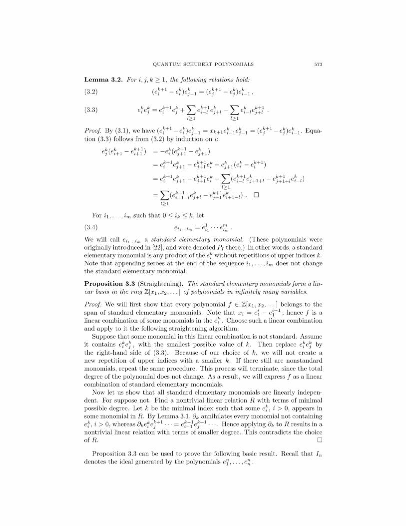
Lemma 3.2. For i, j, k ≥ 1, the following relations hold:
(ek+1i − eki )e
kj−1 = (ek+1
j − ekj )eki−1 ,(3.2)
eki ekj = ek+1
i ekj +∑l≥1
ek+1i−l e
kj+l −
∑l≥1
eki−lek+1j+l .(3.3)
Proof. By (3.1), we have (ek+1i −eki )ekj−1 = xk+1e
ki−1e
kj−1 = (ek+1
j −ekj )eki−1. Equa-
tion (3.3) follows from (3.2) by induction on i:
ekj (eki+1 − ek+1
i+1 ) = −eki (ek+1j+1 − ekj+1)
= ek+1i ekj+1 − ek+1
j+1eki + ekj+1(e
ki − ek+1
i )
= ek+1i ekj+1 − ek+1
j+1eki +
∑l≥1
(ek+1i−l e
kj+1+l − ek+1
j+1+leki−l)
=∑l≥1
(ek+1i+1−le
kj+l − ek+1
j+1eki+1−l) .
For i1, . . . , im such that 0 ≤ ik ≤ k, let
ei1...im = e1i1 · · · emim .(3.4)
We will call ei1...im a standard elementary monomial. (These polynomials wereoriginally introduced in [22], and were denoted PI there.) In other words, a standardelementary monomial is any product of the eki without repetitions of upper indices k.Note that appending zeroes at the end of the sequence i1, . . . , im does not changethe standard elementary monomial.
Proposition 3.3 (Straightening). The standard elementary monomials form a lin-ear basis in the ring Z[x1, x2, . . . ] of polynomials in infinitely many variables.
Proof. We will first show that every polynomial f ∈ Z[x1, x2, . . . ] belongs to thespan of standard elementary monomials. Note that xi = ei1 − ei−1
1 ; hence f is alinear combination of some monomials in the eki . Choose such a linear combinationand apply to it the following straightening algorithm.
Suppose that some monomial in this linear combination is not standard. Assumeit contains eki e
kj , with the smallest possible value of k. Then replace eki e
kj by
the right-hand side of (3.3). Because of our choice of k, we will not create anew repetition of upper indices with a smaller k. If there still are nonstandardmonomials, repeat the same procedure. This process will terminate, since the totaldegree of the polynomial does not change. As a result, we will express f as a linearcombination of standard elementary monomials.
Now let us show that all standard elementary monomials are linearly indepen-dent. For suppose not. Find a nontrivial linear relation R with terms of minimalpossible degree. Let k be the minimal index such that some eki , i > 0, appears insome monomial in R. By Lemma 3.1, ∂k annihilates every monomial not containingeki , i > 0, whereas ∂ke
ki e
k+1j · · · = ek−1
i−1 ek+1j · · · . Hence applying ∂k to R results in a
nontrivial linear relation with terms of smaller degree. This contradicts the choiceof R.
Proposition 3.3 can be used to prove the following basic result. Recall that Indenotes the ideal generated by the polynomials en1 , . . . , e
nn .

574 SERGEY FOMIN, SERGEI GELFAND, AND ALEXANDER POSTNIKOV
Proposition 3.4 (see [22], [23, (2.6)–(2.7)], [25, (4.13)]). Each of the followingform a Z-linear basis in Z[x1, . . . , xn]/In :
• the monomials xa11 · · ·xan−1
n−1 such that 0 ≤ ak ≤ n− k;• the standard elementary monomials ei1i2...in−1 ;• the Schubert polynomials Sw for w ∈ Sn .
Moreover, each of these families spans the same vector space Ln ⊂ Z[x1, . . . , xn] ,which is complementary to In .
Proof. In view of Proposition 2.6, we only need to show that the standard elemen-tary monomials ei1i2...in−1 are linearly independent (this is true by Proposition 3.3)
and span the same space as the monomials xa11 · · ·xan−1
n−1 satisfying 0 ≤ ak ≤ n− k.Indeed, each ei1i2...in−1 is obviously a linear combination of such monomials, andthe result follows by a dimension argument.
3.2. Quantum elementary polynomials. Recall that the quantum elementarypolynomial Ek
i is defined as the coefficient of λi in the characteristic polynomialdet(1 + λGk) of the matrix Gk given by
Gk =
x1 q1 0 · · · 0−1 x2 q2 · · · 00 −1 x3 · · · 0...
......
. . ....
0 0 0 · · · xk
.
By convention, Eki = 0 unless 0 ≤ i ≤ k.
The quantum elementary polynomials Eki have the following combinatorial in-
terpretation. Let us view each variable xj as a singleton j, 1 ≤ j ≤ k, and eachqr as a “dimer” r, r + 1, 1 ≤ r ≤ k − 1. Then Ek
i is the sum of all monomialsin the xj and qr which correspond to disjoint collections of singletons and dimerscovering exactly i distinct nodes. The number of monomials in Ek
k is thus equal tothe k’th Fibonacci number. Also immediate from this description is the recurrence(see [15])
Eki = Ek−1
i + xkEk−1i−1 + qk−1E
k−2i−2 ,(3.5)
for any 1 ≤ i ≤ k, where we assume q0 = 0.The polynomials Ek
i are homogeneous with respect to the grading deg(xi) = 1,deg(qj) = 2, and specialize to the eki in the case q1 = · · · = qn−1 = 0 .
The following analogue of (3.2) can be used for “quantum straightening.”
Lemma 3.5. For k ≥ j ≥ 0, k ≥ i ≥ 0,
Eki E
k+1j+1 + Ek
i+1Ekj + qkE
k−1i−1 E
kj = Ek
j Ek+1i+1 + Ek
j+1Eki + qkE
k−1j−1E
ki .(3.6)
Proof. By (3.5), one has
Eki (Ek+1
j+1 − Ekj+1) = Ek
i (xk+1Ekj + qkE
k−1j−1 )
and
Ekj (Ek+1
i+1 − Eki+1) = Ek
j (xk+1Eki + qkE
k−1i−1 ) .
Subtracting the second equation from the first, we obtain (3.6).

QUANTUM SCHUBERT POLYNOMIALS 575
By analogy with (3.4), we define a quantum standard elementary monomial by
Ei1...im = E1i1 · · ·Em
im ,(3.7)
where 0 ≤ ik ≤ k for k = 1, . . . ,m.The following quantum analogue of Proposition 3.4 can be proved in the same
way as the latter, using a straightening procedure based on Lemma 3.5.
Proposition 3.6. Each of the following form a Z[q]-linear basis in Z[q, x]/Iqn :
• the monomials xa11 · · ·xan−1
n−1 such that 0 ≤ ak ≤ n− k;• the quantum standard elementary monomials Ei1i2...in−1 .
Moreover, each of these two families spans the same vector space Lqn ⊂ Z[q, x]complementary to Iqn .
Quantum straightening can be used to compute the expansion of a product ofseveral quantum standard elementary monomials in the basis Ei1i2...in−1 of thering Z[q, x]/Iqn .
3.3. Quantum Schubert polynomials. Let us recall the combinatorial definitionof the quantum Schubert polynomials Sq
w given in the introduction. By Proposi-tion 3.4, one can uniquely expand an ordinary Schubert polynomial Sw , w ∈ Sn ,as a linear combination of standard elementary monomials, with integer coefficients:Sw =
∑αi1...in−1ei1...in−1 . We then define
Sqw =
∑αi1...in−1Ei1...in−1 .(3.8)
Propositions 3.4 and 3.6 immediately imply the following result.
Proposition 3.7. The quantum Schubert polynomials Sqw for w ∈ Sn , form a
Z[q]-linear basis in the space Lqn spanned by the monomials xa11 · · ·xan−1
n−1 satisfying0 ≤ ak ≤ n − k. The Iqn-cosets of these quantum Schubert polynomials form aZ[q]-linear basis in Z[q, x]/Iqn .
The expansions of Schubert polynomials for Sn in terms of the standard monomi-als can be computed recursively top-down, starting from Swo = e12...n−1 . Namely,use the basic recurrence (2.6) together with the rule for computing a divideddifference of an elementary symmetric polynomial (Lemma 3.1), the Leibniz for-mula (2.4), and the straightening procedure from Section 3.1. For example, in S4
we have:
S4321 = Swo = e123 ,
S3421 = ∂1S4321 = ∂1e123 = e023∂1e11 = e023 ,
S3412 = ∂3S3421 = ∂3e023 = e020∂3e33 = (e22)
2 = e022 − e013 .
The corresponding quantum Schubert polynomials Sqw are then obtained by replac-
ing each standard elementary monomial by its quantum analogue. For instance,
Sq3412 = E022 − E013
= (x1x2 + q1)(x1x2 + x1x3 + x2x3 + q1 + q2)
−(x1 + x2)(x1x2x3 + q1x3 + q2x1)
= x21x
22 + 2q1x1x2 − q2x
21 + q21 + q1q2 .

576 SERGEY FOMIN, SERGEI GELFAND, AND ALEXANDER POSTNIKOV
rrr
rrr
@@@
@@@@
@@
1
x1 x1 + x2
x1x2 + q1 x21 − q1
x21x2 + q1x1
Figure 1. Quantum Schubert polynomials for S3
In Section 14, we provide the tables of quantum Schubert polynomials for S2 ,S3 (cf. Figure 1), and S4 . For each permutation w, we also give the expansionof the Schubert polynomial Sw as a linear combination of standard elementarymonomials.
Proposition 3.8. Sqw is a homogeneous polynomial of degree `(w), with respect to
the grading defined by deg(xi) = 1 and deg(qj) = 2. Specializing q1 = · · · = qn−1 =0 yields Sq
w = Sw , the classical Schubert polynomials.
Proof. The proof follows from the corresponding properties of quantum elementarypolynomials.
Proposition 3.8 implies that the transition matrices between the bases Sqw and
Sw are unipotent triangular, with respect to any linear ordering that is consistentwith the length function `(w).
To conclude this section, we formulate the quantum analogue of the orthogo-nality property (2.9) of the Schubert polynomials. Similarly to the classical case,orthogonality of Schubert classes is a trivial consequence of the quantum cohomol-ogy definitions (cf. Property 9.4 below). At this point, however, we have not provedyet that our combinatorially defined quantum Schubert polynomials Sq
w representSchubert classes σw in the quantum cohomology ring. Moreover, the proof of thisfact given in Section 4 depends on a combinatorial proof of the orthogonality ofthe Sq
w .For F ∈ Z[q, x]/Iqn , let 〈〈F 〉〉 ∈ Z[q] denote the coefficient of Sq
woin the expansion
of F in the basis of quantum Schubert polynomials (cf. Proposition 3.7). Equiva-lently, 〈〈F 〉〉 is the coefficient of the staircase monomial xδ = xn−1
1 xn−22 · · ·xn−1 in
the monomial expansion of F .The following result is the quantum analogue of Theorem 2.9. Its proof is post-
poned until Section 6.
Theorem 3.9 (Orthogonality). For u, v ∈ Sn ,
〈〈Squ Sq
v〉〉 =
1 if v = wou ;
0 otherwise.(3.9)
4. Proof of Theorems 1.1 and 1.2
We begin with an outline of the proof. Let Qw be the “geometric” quantumSchubert polynomials, i.e., the elements of the quotient Z[q, x]/Iqn which represent

QUANTUM SCHUBERT POLYNOMIALS 577
the Schubert classes under the isomorphism (2.15). Theorem 1.2 can be reformu-lated as saying that the Qw coincide with the cosets of the combinatorially definedpolynomials Sq
w .To prove Theorem 1.2 (thus Theorem 1.1), we will need four particular proper-
ties of the elements Qw (see Properties 4.1–4.4). The first three of these propertieseasily follow from the definition of quantum cohomology; the fourth one is a theo-rem of Ciocan-Fontanine [7]. We will use these properties of the Qw , in conjunctionwith several properties of the polynomials Sq
w (most notably, their orthogonality,Theorem 3.9), to demonstrate that the Qw coincide with the cosets of the Sq
w . Asa byproduct, this will immediately imply that Properties 4.1–4.4 uniquely deter-mine the Qw . The issue of axiomatic characterization of the quantum Schubertpolynomials is discussed in Section 9.
In this section, we work in the quotient ring Z[q, x]/Iqn . All polynomials shouldbe understood as representing cosets modulo Iqn .
Property 4.1 (Homogeneity). Every Qw is homogeneous of degree `(w), assum-ing deg(xi) = 1 and deg(qj) = 2.
Proof. See the remark following (2.14).
Property 4.2 (Classical limit). Specializing q1 = · · · = qn−1 = 0 yields Qw =Sw .
Proof. This reflects the fact that this specialization converts the quantum cohomol-ogy of Fln into the usual one.
Properties 4.1 and 4.2 imply that the Qw form a Z[q]-linear basis in Z[q, x]/Iqn ,and the transition matrices between any two of the bases Qw, Sq
w, and Sware unipotent triangular, with respect to any linear ordering consistent with `(w).
The next property is a reformulation of the fact that the Gromov-Witten invari-ants are nonnegative integers.
Property 4.3 (Nonnegativity of structure constants). The structure constants ofthe ring Z[q, x]/Iqn , with respect to the basis Qw , are polynomials in q1, . . . , qn−1
with nonnegative integer coefficients.
Let Z+[q] be the set of all polynomials in the qj whose coefficients are nonnegativeintegers. Let QH∗
+ be the set of all linear combinations of the Qw with coefficientsin Z+[q]. By Property 4.3, QH∗
+ is a semiring, i.e., is closed under addition andmultiplication.
As a corollary, 〈〈Qw1 · · · Qwk〉〉 ∈ Z+[q] , for any w1, . . . , wk ∈ Sn , where 〈〈· · ·〉〉 is
defined as in Section 3.3. Indeed, 〈〈Qw1 · · · Qwk〉〉 is equal to the coefficient of Qwo
in the expansion of this product in the basis Qw , since the transition matrixbetween Qw and Sw is unipotent triangular.
It is well known that the ordinary Schubert polynomial Sw for a cycle w =sk−i+1 · · · sk is the elementary symmetric polynomial eki . The following result,which is a restatement of formula (3) in [7], provides a quantum analogue to thisfact.
Property 4.4 (Quantum elementary polynomials). For a cycle w = sk−i+1 · · · sk∈ Sn , the polynomial Qw is Ek
i , the quantum elementary polynomial.
In our proof of Theorem 1.2, we will only need the following corollary of thisproperty: every quantum elementary polynomial Ek
i belongs to the semiring QH∗+ .
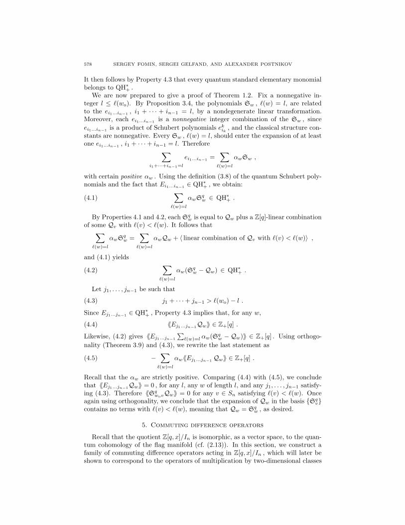
578 SERGEY FOMIN, SERGEI GELFAND, AND ALEXANDER POSTNIKOV
It then follows by Property 4.3 that every quantum standard elementary monomialbelongs to QH∗
+ .We are now prepared to give a proof of Theorem 1.2. Fix a nonnegative in-
teger l ≤ `(wo). By Proposition 3.4, the polynomials Sw , `(w) = l, are relatedto the ei1...in−1 , i1 + · · · + in−1 = l, by a nondegenerate linear transformation.Moreover, each ei1...in−1 is a nonnegative integer combination of the Sw , since
ei1...in−1 is a product of Schubert polynomials ekik , and the classical structure con-stants are nonnegative. Every Sw , `(w) = l, should enter the expansion of at leastone ei1...in−1 , i1 + · · ·+ in−1 = l. Therefore∑
i1+···+in−1=l
ei1...in−1 =∑
`(w)=l
αwSw ,
with certain positive αw . Using the definition (3.8) of the quantum Schubert poly-nomials and the fact that Ei1...in−1 ∈ QH∗
+ , we obtain:∑`(w)=l
αwSqw ∈ QH∗+ .(4.1)
By Properties 4.1 and 4.2, each Sqw is equal to Qw plus a Z[q]-linear combination
of some Qv with `(v) < `(w). It follows that∑`(w)=l
αwSqw =
∑`(w)=l
αwQw + 〈 linear combination of Qv with `(v) < `(w)〉 ,
and (4.1) yields ∑`(w)=l
αw(Sqw −Qw) ∈ QH∗
+ .(4.2)
Let j1, . . . , jn−1 be such that
j1 + · · ·+ jn−1 > `(wo)− l .(4.3)
Since Ej1...jn−1 ∈ QH∗+ , Property 4.3 implies that, for any w,
〈〈Ej1...jn−1Qw〉〉 ∈ Z+[q] .(4.4)
Likewise, (4.2) gives 〈〈Ej1...jn−1
∑`(w)=l αw(Sq
w − Qw)〉〉 ∈ Z+[q] . Using orthogo-
nality (Theorem 3.9) and (4.3), we rewrite the last statement as
−∑
`(w)=l
αw〈〈Ej1...jn−1 Qw〉〉 ∈ Z+[q] .(4.5)
Recall that the αw are strictly positive. Comparing (4.4) with (4.5), we concludethat 〈〈Ej1...jn−1Qw〉〉 = 0 , for any l, any w of length l, and any j1, . . . , jn−1 satisfy-ing (4.3). Therefore 〈〈Sq
wovQw〉〉 = 0 for any v ∈ Sn satisfying `(v) < `(w). Onceagain using orthogonality, we conclude that the expansion of Qw in the basis Sq
vcontains no terms with `(v) < `(w), meaning that Qw = Sq
w , as desired.
5. Commuting difference operators
Recall that the quotient Z[q, x]/In is isomorphic, as a vector space, to the quan-tum cohomology of the flag manifold (cf. (2.13)). In this section, we construct afamily of commuting difference operators acting in Z[q, x]/In , which will later beshown to correspond to the operators of multiplication by two-dimensional classes
QUANTUM SCHUBERT POLYNOMIALS 579
in the ring QH∗(Fln,Z). These operators will be an essential tool in our proof ofthe orthogonality property, needed for the proof of Theorem 1.2.
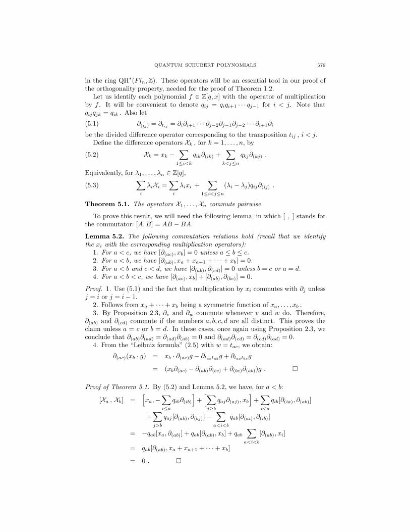
Let us identify each polynomial f ∈ Z[q, x] with the operator of multiplicationby f . It will be convenient to denote qij = qiqi+1 · · · qj−1 for i < j. Note thatqijqjk = qik . Also let
∂(ij) = ∂tij = ∂i∂i+1 · · · ∂j−2∂j−1∂j−2 · · · ∂i+1∂i(5.1)
be the divided difference operator corresponding to the transposition tij , i < j.Define the difference operators Xk , for k = 1, . . . , n, by
Xk = xk −∑
1≤i<kqik∂(ik) +
∑k<j≤n
qkj∂(kj) .(5.2)
Equivalently, for λ1, . . . , λn ∈ Z[q],∑i
λiXi =∑i
λixi +∑
1≤i<j≤n(λi − λj)qij∂(ij) .(5.3)
Theorem 5.1. The operators X1, . . . ,Xn commute pairwise.
To prove this result, we will need the following lemma, in which [ , ] stands forthe commutator: [A,B] = AB −BA.
Lemma 5.2. The following commutation relations hold (recall that we identifythe xi with the corresponding multiplication operators):
1. For a < c, we have [∂(ac), xb] = 0 unless a ≤ b ≤ c.2. For a < b, we have [∂(ab), xa + xa+1 + · · ·+ xb] = 0.3. For a < b and c < d, we have [∂(ab), ∂(cd)] = 0 unless b = c or a = d.4. For a < b < c, we have [∂(ac), xb] + [∂(ab), ∂(bc)] = 0.
Proof. 1. Use (5.1) and the fact that multiplication by xi commutes with ∂j unlessj = i or j = i− 1.
2. Follows from xa + · · ·+ xb being a symmetric function of xa, . . . , xb .3. By Proposition 2.3, ∂v and ∂w commute whenever v and w do. Therefore,
∂(ab) and ∂(cd) commute if the numbers a, b, c, d are all distinct. This proves theclaim unless a = c or b = d. In these cases, once again using Proposition 2.3, weconclude that ∂(ab)∂(ad) = ∂(ad)∂(ab) = 0 and ∂(ad)∂(cd) = ∂(cd)∂(ad) = 0.
4. From the “Leibniz formula” (2.5) with w = tac, we obtain:
∂(ac)(xb · g) = xb · ∂(ac)g − ∂tactabg + ∂tactbcg
= (xb∂(ac) − ∂(ab)∂(bc) + ∂(bc)∂(ab))g .
Proof of Theorem 5.1. By (5.2) and Lemma 5.2, we have, for a < b:
[Xa , Xb] =[xa,−
∑i≤a
qib∂(ib)
]+[∑j≥b
qaj∂(aj), xb
]+∑i<a
qib[∂(ia), ∂(ab)]
+∑j>b
qaj [∂(ab), ∂(bj)]−∑
a<i<b
qab[∂(ai), ∂(ib)]
= −qab[xa, ∂(ab)] + qab[∂(ab), xb] + qab∑
a<i<b
[∂(ab), xi]
= qab[∂(ab), xa + xa+1 + · · ·+ xb]
= 0 .

580 SERGEY FOMIN, SERGEI GELFAND, AND ALEXANDER POSTNIKOV
For a polynomial f ∈ Z[q, x], we write f(X ) to denote the operator f(X1, . . . ,Xn);this is well defined by Theorem 5.1. Accordingly, f(X )(g) will denote the result ofapplying f(X ) to a polynomial g.
Lemma 5.3. For any polynomial f ∈ Z[q, x] , there exists a unique F ∈ Z[q, x]such that f = F (X )(1).
Proof. Let degx denote the degree on Z[q, x] defined by degx(xi) = 1 and degx(qj) =0. We first prove existence by induction on degx(f) = d. If d = 0, then f ∈ Z[q]and F = f . Suppose d > 0. Since each operator Xi − xi lowers degx , it followsthat f(x) − f(X )(1) is a polynomial of degree < d. By the induction assumption,this polynomial can be expressed in the form g(X )(1), for some g ∈ Z[q, x]. Hencef(x) = (f + g)(X )(1) . To prove uniqueness, note that whenever h 6= 0, one hasdegx(h(X )(1)) = degx(h) ≥ 0, implying h(X )(1) 6= 0.
As a corollary of the last lemma, commuting operators X1, . . . ,Xn are alge-braically independent over the ring Z[q].
By Lemma 5.3, we have a Z[q]-linear bijection ψ : Z[q, x] → Z[q, x] given by
ψ : f 7→ F , f = F (X )(1) .(5.4)
Our next goal is to find the polynomial F = ψ(f) for the special case f = ei1,...,im .
Proposition 5.4. We have Eki (X )(g) = eki g for any polynomial g ∈ Z[q, x] which
is symmetric in the variables x1, . . . , xk+1 , k < n, and also in the case g = 1,k = n.
Proof. Induction on k. If k = 0, then E00(X )(g) = e00 g = g. Suppose k > 0. Then,
using the induction hypothesis, Lemma 3.1, (3.1), and (3.5), we obtain:
Eki (X )(g) =
(Ek−1i (X ) + XkE
k−1i−1 (X ) + qk−1E
k−2i−2 (X )
)(g)
= ek−1i g + Xk(e
k−1i−1 g) + qk−1e
k−2i−2 g
= ek−1i g + xke
k−1i−1 g − qk−1∂k−1e
k−1i−1 g + qk−1e
k−2i−2 g
= ek−1i g + xke
k−1i−1 g
= eki g .
Theorem 5.5. For any m ≤ n, we have Ei1...im(X )(1) = ei1...im . In particular,Eki (X )(1) = eki for any i ≤ k ≤ n.Equivalently, ψ(ei1...im) = Ei1...im and ψ(eki ) = Ek
i , in the notation of (5.4).
Proof. Repeatedly using Proposition 5.4, we obtain:
Ei1...im(X )(1) = Ei1...im−1(X )(emim)
= Ei1...im−2(X )(em−1im−1
emim) = · · · = e1i1 · · · emim .
Corollary 5.6. For any w ∈ Sn , we have ψ(Sw) = Sqw , i.e., Sq
w(X )(1) = Sw .
Proof. The proof follows from the definition (3.8) of quantum Schubert polynomials.

QUANTUM SCHUBERT POLYNOMIALS 581
Lemma 5.7. The map ψ defined by (5.4) bijectively maps the ideal In onto Iqn .
Proof. Every element in In is of the form f1e1n+ · · ·+fne
nn , for f1, . . . , fn ∈ Z[q, x].
Denote Fi = ψ(fi) . Note that each operator Xi commutes with multiplication byany polynomial which is symmetric in x1, . . . , xn (cf. Proposition 2.4 and (5.2)).Using this observation together with Theorem 5.5, we obtain: (FiE
ni )(X )(1) =
Fi(X )(eni ) = eni Fi(X )(1) = eni fi. Hence ψ(f1en1 + · · ·+fnenn) = F1E
n1 + · · ·+FnEn
n ,proving the lemma.
By Lemma 5.7 and Theorem 5.5, the map ψ induces a Z[q]-linear bijection
Z[q, x]/In → Z[q, x]/Iqn ,(5.5)
which sends the cosets of the ei1...im to the corresponding cosets of Ei1...im .
Lemma 5.8. The operators X1, . . . ,Xn leave the space In ⊂ Z[q, x] invariant.
Proof. We have Xi(f1en1 + · · ·+ fne
nn) = en1Xi(f1) + · · ·+ ennXi(fn) .
Observe that the definition (5.4) of the map ψ implies that Xi(g) = ψ−1(xiψ(g))for any polynomial g. In other words, ψ translates the action of Xi into mul-tiplication by xi . In view of Lemma 5.8, Xi induces an operator in Z[q, x]/In .This operator corresponds via ψ to multiplication by xi in the ring Z[q, x]/Iqn .It follows that the Xi , understood as operators acting in Z[q, x]/In , satisfy therelations Ek(X ) = 0, and thus provide a representation for the ring QH(Fln,Z).
We conclude this section by a useful corollary of Theorem 5.5 and formula (2.7).
Corollary 5.9. Let F ∈ Z[q, x]/Iqn . Then 〈〈F 〉〉 is equal to the constant term of∂wo(F (X )(1)). (The latter is well defined by Lemma 5.7.)
6. Proof of orthogonality
In this section we prove the orthogonality property of the quantum Schubertpolynomials (Theorem 3.9). To this end, we will need the following lemmas. Asbefore, we identify polynomials with the corresponding multiplication operators.
Lemma 6.1. Let l ≤ k < n. Then, for any i1, . . . , ik−1 ,
∂woe1i1 · · · ek−1
ik−1∂l∂l+1 · · · ∂k = 0 .(6.1)
Proof. Let us move ∂l, . . . , ∂k to the left, one by one. By Lemma 3.1 and Proposi-tion 2.4, ∂m commutes with eai unless m = a, whereas
emi ∂m = ∂mei(x1, . . . , xm−1, xm+1) + em−1i−1 .(6.2)
If ∂m moves through emim (the first term in the right-hand side of (6.2)), then itcan be moved all the way to the left, and the corresponding term vanishes since∂wo∂m = 0. Otherwise ∂m changes emim into em−1
i−1 . The only term remaining in theleft-hand side of (6.1) upon moving ∂l, . . . , ∂k−1 will be
∂woe1i1 · · · el−1
il−1el−1il−1 · · · ek−2
ik−1−1∂k = ∂wo∂ke1i1 · · · el−1
il−1el−1il−1 · · · ek−2
ik−1−1 = 0 .
Recall that Lqn denotes the Z[q]-span of the monomials xa11 · · ·xan−1
n−1 such that0 ≤ ai ≤ n− i for all i. By Proposition 3.4, the polynomials ei1...in−1 form a Z[q]-basis of Lqn . The following result is proved in exactly the same way as Theorem 5.5.

582 SERGEY FOMIN, SERGEI GELFAND, AND ALEXANDER POSTNIKOV
Proposition 6.2. For any f ∈ Lqn and any polynomial g which is symmetric inx1, . . . , xn , we have F (X )(g) = G(X )(f) = fg, where F = ψ(f) and G = ψ(g), inthe notation of (5.4).
Let us fix an integer k such that 1 ≤ k ≤ n. It will be convenient to represent
the operators Xl , l ≤ k, in the form Xl = Xl +≈X l, where
Xl = xl −∑j<l
qjl∂(jl) +∑
l<j≤kqlj∂(lj) ,
≈X l =
∑j>k
qlj∂(lj) .(6.3)
Let Eki (X ) = Ek
i (X1, . . . , Xk).
Proposition 6.3. For any polynomial f ∈ Z[q, x] ,
Eki (X )(f) = eki f .(6.4)
Thus Eki (X ) coincides with the operator of multiplication by eki , provided qk = 0.
Proof. Let us denote Pk = Z[q1, . . . , qk−1][x1, . . . , xk]. The operator Eki (X ) does
not involve divided differences ∂l with l ≥ k. Therefore it commutes with xl , l > k,
and it suffices to prove (6.4) for f ∈ Pk . (Notice that in this case Eki (X )(f) ∈ Pk .)
Let us expand f in the standard elementary monomials (possibly involving vari-ables xl with l > k). Let N be greater than the largest value of M such that someeMi enters one of these monomials. Then f ∈ LqN and, by Proposition 6.2, we haveENi (X )(f) = eNi f . The ideal Jk = 〈qk, qk+1, . . . , xk+1, xk+2, . . . 〉 is an invariant
subspace for all the Xi and for the operators of multiplication by xi . Hence Xi andxi act on the quotient space, which is isomorphic to Pk . The corresponding actions
of ENi (X ) and eNi on Pk coincide with Ek
i (X ) and eki , respectively. This implies
Eki (X )(f) = eki f , as desired.
Lemma 6.4. For any k < n and any f ,
∂woei1...ik−1(Ek
ik(X ) − ekik) f = 0 .(6.5)
Proof. Let us write Ekik
(X ) as a polynomial in the Xl , l ≤ k, substitute Xl = Xl+≈X l
everywhere, and expand. The terms which only involve the truncated operators Xl
will combine into the operator Ekik
(X ). By Proposition 6.3, (Ekik
(X ) − ekik)f = 0 .To prove Lemma 6.4, it therefore suffices to show that any composition of operatorsof the form
∂woei1...ik−1Xl1 · · · Xlj∂(lm) ,(6.6)
with 1 ≤ l1 < l2 < · · · < lj < l ≤ k < m, vanishes. In view of the definitionof ∂(lm) , this claim will follow if we prove that
∂woei1...ik−1Xl1 · · · Xlj∂l · · · ∂k = 0(6.7)
for 1 ≤ l1 < l2 < · · · < lj < l ≤ k. We will prove (6.7) by induction on j. If j = 0,then it coincides with Lemma 6.1. For j > 0, the only term in the expression (6.3)
for Xlj that neither commutes with (∂l · · · ∂k) nor vanishes after composition with(∂l · · · ∂k) is qlj l∂(lj l) . We then note that
∂(lj l)(∂l · · · ∂k) = ∂lj · · · ∂l−2∂l−1∂l−2 · · · ∂lj (∂l · · · ∂k) = (∂lj · · ·∂k)∂l−2 · · · ∂lj .

QUANTUM SCHUBERT POLYNOMIALS 583
Using the induction assumption, we conclude that the left-hand side of (6.7) equals
qlj l (∂woei1...ik−1Xl1 · · · Xlj−1∂lj∂lj+1 · · · ∂k)∂l−2 · · ·∂lj .
The parenthesized factor is an expression similar to the left-hand side of (6.7) withj decreased by 1 and l replaced by lj . By the induction assumption, it vanishes,and Lemma 6.4 is proved.
We will now complete the proof of Theorem 3.9. Let us first note that the onlynontrivial case is `(u)+ `(v) > `(wo). Indeed, if deg(Sq
u Sqv) = `(u)+ `(v) < `(wo),
then the monomial xδ cannot appear in the expansion of Squ Sq
v . In the case`(u)+ `(v) = `(wo), the only terms which can contribute to 〈〈Sq
u Sqv〉〉 are those not
involving the qi , and (3.9) follows from its classical counterpart (2.9).Since our quantum Schubert polynomials are linear combinations of quantum
standard elementary monomials of the same degree, it remains to show that
〈〈Ei1...in−1 Ej1...jn−1〉〉 = 0(6.8)
whenever
i1 + · · ·+ in−1 + j1 + · · ·+ jn−1 > `(wo) = n(n− 1)/2 .(6.9)
In view of Theorem 5.5, Ei1...in−1(X )Ej1...jn−1(X )(1) = Ei1...in−1(X )(ej1...jn−1). ByCorollary 5.9, formula (6.8) is equivalent to
(∂wo(Ei1...in−1(X )(ej1...jn−1)))(0, . . . , 0) = 0 .(6.10)
Suppressing (X ) to avoid cumbersome notation, let us write
Ei1...in−1 = E1i1 · · ·En−1
in−1=
(e1i1 + (E1
i1 − e1i1)
)· · ·(en−1in−1
+ (En−1in−1
− en−1in−1
)
)and prove that for each term T in the expansion of this product we have
(∂woT (ej1...jn−1))(0, . . . , 0) = 0 .(6.11)
If T = e1i1 · · · en−1in−1
, then (6.11) follows from (6.9). Any other T is of the form
T = e1i1 · · · ek−1ik−1
(Ekik − ekik)T
′
for some k ≤ n−1, and (6.11) follows from Lemma 6.4 with g = T ′(ej1...jn−1). Thiscompletes the proof of Theorem 3.9.
Define a bilinear form ( , ) in Z[q, x]/Iqn by setting
(F,Sqw) = 〈〈F Sq
wow〉〉 .(6.12)
The following result is a reformulation of Theorem 3.9.
Theorem 6.5. With respect to the scalar product(6.12) in Z[q, x]/Iqn , the quantumSchubert polynomials Sq
w , w ∈ Sn , form an orthonormal basis.

584 SERGEY FOMIN, SERGEI GELFAND, AND ALEXANDER POSTNIKOV
7. Quantum Monk’s formula
In this section, we prove the quantum Monk’s formula (Theorem 1.3). Let usfirst reformulate this formula in the language of quantum Schubert polynomials.
Theorem 7.1 (Quantum Monk’s formula). For w ∈ Sn and 1 ≤ r < n,
Sqsr Sq
w = (x1 + · · ·+ xr)Sqw =
∑Sqwtab
+∑
qcdSqwtcd
,(7.1)
where the first sum is over all transpositions tab such that a ≤ r < b and `(wtab) =`(w) + 1, and the second sum is over all transpositions tcd such that c ≤ r < d and`(wtcd) = `(w) − `(tcd) = `(w)− 2(d− c) + 1.
More generally, for any linear form f =∑λixi , one has
fSqw =
∑(λa − λb)S
qwtab +
∑(λc − λd)qcdS
qwtcd ,(7.2)
where the sums are over a < b and c < d such that `(wtab) = `(w) + 1 and`(wtcd) = `(w) − `(tcd), respectively.
Proof. By the classical Monk’s formula (Theorem 2.8), the definition of Sqw , and
Theorem 5.5, the equation (7.2) is equivalent to
f(X )(Sw) = f ·Sw +∑
(λc − λd)qcdSwtcd ,
summed over all c < d such that `(wtcd) = `(w) − `(tcd). The latter follows fromCorollary 2.7.
Notice that formulas (7.1) and (7.2) hold on the level of polynomials, not justfor cosets (classes), as in Theorem 1.3.
8. Quantization map
At this point, let us review our main results, now that all of them are proved.In view of Theorems 1.1, 5.5 (cf. also (5.5)) and 7.1, we now have four differ-
ent descriptions of the quantization map Z[q, x]/In → Z[q, x]/Iqn defined by thecommutative diagram (1.5). Geometrically, this is the map that sends a cosetthat corresponds to a given class in the ordinary cohomology of Fln to the cosetcorresponding to the same class as an element of the quantum cohomology ring.Algebraically (or combinatorially), this map is defined by its action on standardelementary monomials:
ei1...in−1 7−→ Ei1...in−1 .
The quantization map can also be defined in terms of the operators Xk givenby (5.2). Namely, the quantization image F of f is uniquely determined by
f = (F (X1, . . . ,Xn))(1) .
Yet another description can be obtained from the quantum Monk’s formula. It isnot hard to see that this formula can be used to recursively obtain the quantumSchubert polynomials, starting with S
q1 = 1. The quantization map is then defined
by
Sw 7−→ Sqw .
QUANTUM SCHUBERT POLYNOMIALS 585
9. Axiomatic characterization
In Section 4, we have actually proved the following characterization theorem.
Theorem 9.1. Let Qww∈Sn be a family of elements of Z[q, x]/Iqn satisfying Prop-erties 4.1–4.4. Then the Qw are the cosets of the quantum Schubert polynomi-als Sq
w .
It is natural to ask exactly which properties are essential to uniquely determinethe elements Qw . In particular, does one really need Property 4.4, which is theonly property in Theorem 9.1 that does not immediately follow from the definitionof the quantum cohomology of Fln ?
Proposition 9.2. In the case of S3 (or Fl3), Properties 4.1–4.3 uniquely deter-mine the Qw (which hence coincide with the cosets of the Sq
w).
Proof. We certainly know that Q1 = 1, Qs1 = x1 , and Qs2 = x1 + x2 . Assumethat Qs1s2 = Sq
s1s2 +a and Qs2s1 = Sqs2s1 +b , where a and b are, by Properties 4.1
and 4.2, some linear combinations of q1 and q2 . Then direct computations (with or
without a computer) give 〈〈Qs1s2 (Qs1)2Qs2 〉〉 = a and 〈〈Qs2s1 (Qs2)
2Qs1 〉〉 = b ,implying that both a and b are nonnegative linear combinations of q1 and q2 (wewill simply write a ≥ 0 and b ≥ 0). On the other hand,
Qs1Qs2 = x1(x1 + x2) = Sqs1s2 + Sq
s2s1 = Qs1s2 +Qs2s1 + (−a− b) .
Hence −a − b ≥ 0 and therefore a = b = 0, as desired. The remaining case ofQwo is treated in analogous fashion. Assume Qwo = Sq
wo+ cSq
s1 + dSqs2 . Then
〈〈QwoQs1s2 〉〉 = 〈〈QwoSqs1s2 〉〉 = c and 〈〈QwoQs2s1 〉〉 = 〈〈QwoS
qs2s1 〉〉 = d , implying
c ≥ 0 and d ≥ 0. On the other hand, Qs1Qs1s2 = Sqwo
= Qwo − cQs1 − dQs2 .Hence −c ≥ 0 and −d ≥ 0, and therefore c = d = 0, as desired.
Similar but more involved considerations allowed us to verify, with the help ofa computer, that the result analogous to Proposition 9.2 holds for n = 4. It istempting to conjecture that this holds for every n. This would be a very nice result(perhaps too nice to be true), since it would mean that it suffices to use the basicproperties of quantum cohomology to uniquely determine the polynomials Sq
w .
Conjecture 9.3 (Strong version). The quantum Schubert polynomials are unique-ly defined by Properties 4.1–4.3. In other words, they are the only elements ofZ[q, x]/Iqn which are homogeneous with respect to the grading deg(xi) = 1, deg(qj) =2, specialize to the ordinary Schubert polynomials in the classical limit q1 = · · · =qn−1 = 0, and whose structure constants are polynomials in the qi with nonnegativeinteger coefficients.
A weaker conjecture (cf. Conjecture 9.7 below) would extend the defining setof axioms by additional properties of the elements Qw , which can be directly de-rived from the their geometric definition. The first of these extra properties isorthogonality (cf. Theorem 3.9).
Property 9.4. For u, v ∈ Sn ,
〈〈QuQv〉〉 =
1 if v = wou ;
0 otherwise.(9.1)

586 SERGEY FOMIN, SERGEI GELFAND, AND ALEXANDER POSTNIKOV
Proof. By definition, 〈〈QuQv〉〉 is the coefficient of Qwo in QuQv , which is equal tothe coefficient of the Schubert cycle σwo in the quantum product σu ∗ σv . In viewof (2.14) and the S3-symmetry of the Gromov-Witten invariants, this is the sameas the coefficient of σwou in σv ∗ σ1 = σv , which obviously equals the right-handside of (9.1).
The S2-symmetry of the type An−1 Dynkin diagram has as a consequence theinvariance of the quantum (and, in particular, the ordinary) cohomology of theflag manifold with respect to the involutive ring automorphism ω : QH∗(Fln) →QH∗(Fln) defined by ω(σsk) = σsn−k and ω(qk) = qn−k for k = 1, 2, . . . , n − 1.Since Qsk = Sq
sk = x1 + · · · + xk , and x1 + · · · + xn ∈ Iqn , we can alternativelydefine ω as the ring automorphism of Z[q, x]/Iqn given by
ω(xk) = −xn+1−k , ω(qk) = qn−k .(9.2)
Property 9.5. For any w ∈ Sn , one has ω(Qw) = Qwowwo .
The involution ω is studied in Section 11.1. In particular, Property 9.5 can beproved combinatorially (cf. Corollary 11.6).
Property 9.6. If u and v belong to the parabolic subgroups generated by s1, . . . , skand sk+1, . . . , sn−1 , respectively, for some k, then Quv = QuQv .
Conjecture 9.7 (Weak version). The quantum Schubert polynomials are uniquelydefined by Properties 4.1–4.3 and 9.4–9.6.
10. Stability
The quantum Schubert polynomials have an important stability property thatjustifies their choice as specific polynomial representatives of the correspondingcosets modulo the ideal Iqn . Consider the natural embeddings of the symmetricgroups S1 ⊂ S2 ⊂ S3 ⊂ · · · ; viz., Sn permutes the set 1, . . . , n.Theorem 10.1 (Stability). Let w ∈ Sn . The quantum Schubert polynomial Sq
w isthe unique polynomial in Z[q1, . . . , qn−1][x1, . . . , xn] which has the following prop-erty: for every N ≥ n, the polynomial Sq
w represents the Schubert class σw , in thequantum cohomology ring QH∗(FlN ) ∼= Z[q1, . . . , qN−1][x1, . . . , xN ]/IqN .
Proof. It is immediate from our definition that the quantum Schubert polynomialSqw , for w ∈ Sn , does not change if w is regarded as an element of SN , for any
N > n. Hence the property in question follows from Theorem 1.2. To proveuniqueness, it suffices to show that if a polynomial f ∈ Z[q1, . . . , qn−1][x1, . . . , xn]vanishes modulo the ideal IqN , for all N > n, then it vanishes identically. Indeed, fbelongs to the Z[q1, . . . , qN−1]-span of the monomials xa1
1 · · ·xaN−1
N−1 , 0 ≤ ak ≤ N−k,for N ≥ n+ degx(f). Therefore, by Proposition 3.6, f = 0 if f ∈ IqN .
Several properties of the quantum Schubert polynomials Sqw are peculiar to the
particular choice of coset representatives that we made. The proofs of the followingstatements are left to the reader:
• the quantum Schubert polynomials Sqw , for w ∈ S∞ , where S∞ =
⋃Sn , form
a Z[q1, q2, . . . ]-linear basis of the polynomial ring Z[q1, q2, . . . ][x1, x2, . . . ];• to multiply Sq
u and Sqv in the quotient ring Z[q, x]/Iqn (which is equivalent
to computing the quantum product σu ∗ σv of the corresponding Schubertclasses), expand Sq
u Sqv in the basis Sq
w of the ring Z[q1, q2, . . . ][x1, x2, . . . ]and drop all terms containing Sq
w with w not in Sn ;
QUANTUM SCHUBERT POLYNOMIALS 587
• Sqw does not involve qn−1 ;
• if w ∈ Sn but w /∈ Sn−1 , then Sqw ∈ Iqn−1 .
11. Miscellaneous
11.1. Quantum complete homogeneous polynomials. Let hkl denote the sumof all monomials of degree l in the variables x1, . . . , xk (the complete homogeneoussymmetric polynomial). The following result is well known.
Lemma 11.1. For k + l > n, one has hkl ∈ In .
Proof. The statement follows from the formula hkl = det(ek+l−ij−i+1
)li, j=1
since all
elements in the first row of this determinant belong to In .
The proofs of the remaining results in Section 11 are fairly straightforward, andare omitted for the sake of brevity.
Theorem 11.2. The quantization map sends the coset of a complete homogeneous
polynomial hkl to Hkl = det
(Ek+l−ij−i+1
)li, j=1
. More generally, the quantization of
hi1...in−1 = h1i1· · ·hn−1
in−1, where ik ≤ n− k for k = 1, . . . , n− 1, is
Hi1...in−1 = H1i1 · · ·Hn−1
in−1.(11.1)
Observe that if the condition ik ≤ n − k is not satisfied for at least one valueof k, then hi1...in−1 ∈ In , by Lemma 11.1.
The quantum complete homogeneous polynomials Hkl will play a role in Sec-
tion 12.1 as elements of a Grobner basis for the ideal Iqn . These polynomials can begiven a direct combinatorial interpretation in terms of families of nonintersectingpaths in a certain oriented graph.
11.2. Involution ω. Let ω be the involutive automorphism of the polynomialring Z[q, x] defined by ω(xk) = −xn+1−k and ω(qk) = qn−k , for k = 1, . . . , n(cf. (9.2)).
Lemma 11.3. Both In and Iqn are invariant subspaces for the involution ω.
This shows that ω has well-defined actions on both Z[q, x]/In and Z[q, x]/Iqn .
Proposition 11.4 (cf. [21]). In Z[q, x]/In , the following rules for computing ω-images hold:
ω(ei1...in−1) = hin−1...i1 ; ω(hi1...in−1) = ein−1...i1 ; ω(Sw) = Swowwo .
Proposition 11.5. Involution ω commutes with the quantization map.
Corollary 11.6. In Z[q, x]/Iqn , the following rules for computing ω-images hold:
ω(Ei1...in−1) = Hin−1...i1 ; ω(Hi1...in−1) = Ein−1...i1 ; ω(Sqw) = Sq
wowwo.
11.3. Quantization of square-free monomials. The combinatorial construc-tion of Section 3.2 can be used to describe the image of any square-free monomialxa = xa1xa2 · · · under the quantization map. Consider the graph whose verticesare the ai and whose edges connect ai and aj if |ai − aj | = 1. Assign weight xai tothe vertex ai and weight qai to the edge (ai, ai + 1). Then every matching in thisgraph (a collection of vertex-disjoint edges) acquires a weight equal to the productof weights of its edges multiplied by the weights of remaining vertices. The sum of

588 SERGEY FOMIN, SERGEI GELFAND, AND ALEXANDER POSTNIKOV
these weights, for all matchings, is the quantization of the monomial xa . A similarrule for computing the inverse (“dequantization”) image Xa1Xa2 · · · (1) of a square-free monomial xa can be obtained using Mobius inversion. The only difference fromthe quantization rule is in replacing each qi by −qi .
12. Explicit computation
12.1. Grobner bases. Recall that Lqn denotes the space, complementary to theideal Iqn , which is spanned (over Z[q]) by the monomials xa1
1 · · ·xan−1
n−1 satisfying0 ≤ ak ≤ n − k. Another basis of Lqn is formed by the quantum Schubert poly-nomials Sq
w , for w ∈ Sn (see Proposition 3.7). The problem of finding the uniquerepresentative in Lqn of a given coset modulo Iqn can be solved using Grobner basestechniques. We refer the reader to [29, Chapter 1], which contains all definitionsand facts that we will need from the theory of Grobner bases.
Let us use the degree lexicographic order, induced from x1 ≺ x2 ≺ · · · ≺ xn , onthe set of all monomials xa1
1 · · ·xann . More precisely, we first order the monomialsby the total degree a1 + · · · + an , and then break the ties using the lexicographicorder on the sequences (an, . . . , a1). This allows us to introduce the normal formof any polynomial with respect to the ideal Iqn and the monomial order specifiedabove. This normal form can be found by means of a reduction procedure versusthe corresponding reduced Grobner basis G of Iqn . The following direct descriptionof this Grobner basis and the space of normal forms can be viewed as the quantumanalogue of [29, Theorem 1.2.7].
Proposition 12.1. The vector space Lqn is the space of normal forms for the idealIqn ⊂ Z[q, x] with respect to the degree lexicographic monomial order defined above.
The corresponding reduced Grobner basis G consists of the quantum completehomogeneous polynomials Hn+1−k
k , k = 1, . . . , n (see Theorem 11.2).
Proof. We already know that each coset modulo Iqn contains a unique representativefrom Lqn . Let us show that any monomial outside Lqn is congruent modulo Iqn toa sum of smaller monomials. Assume xa = xa1
1 · · ·xann /∈ Lqn , which means thatak > n − k for some k. Then, by Lemma 11.1, hkak ∈ In , implying Hk
ak∈ Iqn .
Note that xakk is the largest monomial in the expansion of Hkak . Hence xakk can be
written, modulo Iqn , as a linear combination of smaller monomials. Multiplying byall the xaii with i 6= k, we obtain the desired expansion of xa into smaller terms.
The description of the Grobner basis G is then derived from the following twofacts: (i) the monomials outside Lqn are exactly those divisible by some monomial
of the form xkn+1−k , and (ii) a leading monomial of Hn+1−kk is xkn+1−k .
To illustrate, for n = 3 the space of normal forms is the Z[q1, q2]-span of themonomials 1, x1, x
21, x2, x1x2, x
21x2 . The reduced minimal Grobner basis for Iq3
consists of
H31 = x1 + x2 + x3 ,
H22 = x2
1 + x1x2 + x22 − q1 − q2 ,
and
H13 = x3
1 − 2x1q1 − x2q1 .
QUANTUM SCHUBERT POLYNOMIALS 589
12.2. Computing the Gromov-Witten invariants. Since the quantum Schu-bert polynomials Sq
w represent Schubert classes, the structure constants of thering Z[q, x]/Iqn with respect to the basis Sq
w are the generating functions for theGromov-Witten invariants 〈σu, σv, σw〉d of the flag manifold (cf. (2.14)). Actually,(2.14) generalizes to
σw1 ∗ · · · ∗ σwk=∑w∈Sn
∑d
qd 〈σw, σw1 , . . . , σwk〉d σwow(12.1)
(see, e.g., [7]). This formula allows us to compute k-point Gromov-Witten invariantsfor an arbitrary k.
Corollary 12.2. For any w1, . . . , wk ∈ Sn ,
〈〈Sqw1· · ·Sq
wk〉〉 =
∑d
qd〈σw1 , . . . , σwk〉d .(12.2)
Proof. This is a consequence of (12.1) and the orthogonality property (3.9).
Combining (12.2) with Corollary 5.9, we obtain the following formula for thegenerating function of the Gromov-Witten invariants.
Corollary 12.3. For any w1, . . . , wk ∈ Sn ,
∑d
qd〈σw1 , . . . , σwk〉d =
⟨∏j
Sqwj
(X1, . . . ,Xn−1)
(1)
⟩,(12.3)
where 〈f〉 denotes the constant term of ∂wo(f) (cf. (2.7) and(2.8)).
An efficient alternative to the last formula is provided by a method describedbelow, which is based on the Grobner bases techniques developed in Section 12.1.
Corollary 12.4. The expansion of an element F ∈ Z[q, x]/Iqn in the basis of cosetsof quantum Schubert polynomials Sq
w , w ∈ Sn , is given by F =∑cwSq
w mod Iqn ,where each cw is the coefficient of the staircase monomial xδ = xn−1
1 xn−22 · · ·xn−1
in the normal form of the polynomial FSqwow with respect to the degree lexicographic
monomial order described in Section 12.1.
Proof. In view of Theorem 3.9, cw is equal to the coefficient of Sqwo
in the expansionof FSq
wow . By Proposition 12.1, the normal form of FSqwow lies in Lqn , and the
coefficient of Sqwo
in its expansion in the basis of quantum Schubert polynomials is
equal to the coefficient of xδ .
Theorem 12.5. A Gromov-Witten invariant 〈σw1 , . . . , σwk〉d of the flag manifold
is the coefficient of the monomial qd xδ in the normal form, with respect to thedegree lexicographic order induced from x1 ≺ x2 ≺ x3 ≺ · · · , of the product ofquantum Schubert polynomials Sq
w1· · ·Sq
wk. This normal form can be found using
the reduction procedure versus the Grobner basis G = Hn1 , H
n−12 , . . . , H2
n−1, H1n.
Proof. The proof follows from Corollaries 12.2 and 12.4 and Proposition 12.1.
590 SERGEY FOMIN, SERGEI GELFAND, AND ALEXANDER POSTNIKOV
We remark that it is usually more efficient to alternate normal form reductionwith multiplication by Sq
w1, Sq
w2, . . . .
The cases k = 1, 2 of Theorem 12.5 are not so interesting, since the only non-vanishing values are 〈σwo〉(0,...,0) = 1 and 〈σu , σwou〉(0,...,0) = 1, for any u ∈ Sn .The case k = 3 is nontrivial and actually determines all other invariants, becauseof the associativity property of quantum multiplication. Theorem 12.5 provides amethod to directly calculate the invariants 〈σw1 , . . . , σwk
〉d for arbitrary k, avoidingthe use of associativity. For example—just to show the practical efficiency of thealgorithms—one has, in Fl4 , 〈σwo , . . . , σwo︸ ︷︷ ︸
17
〉(15,19,14) = 385056 .
13. Gromov-Witten invariants for Fl3 and Fl4
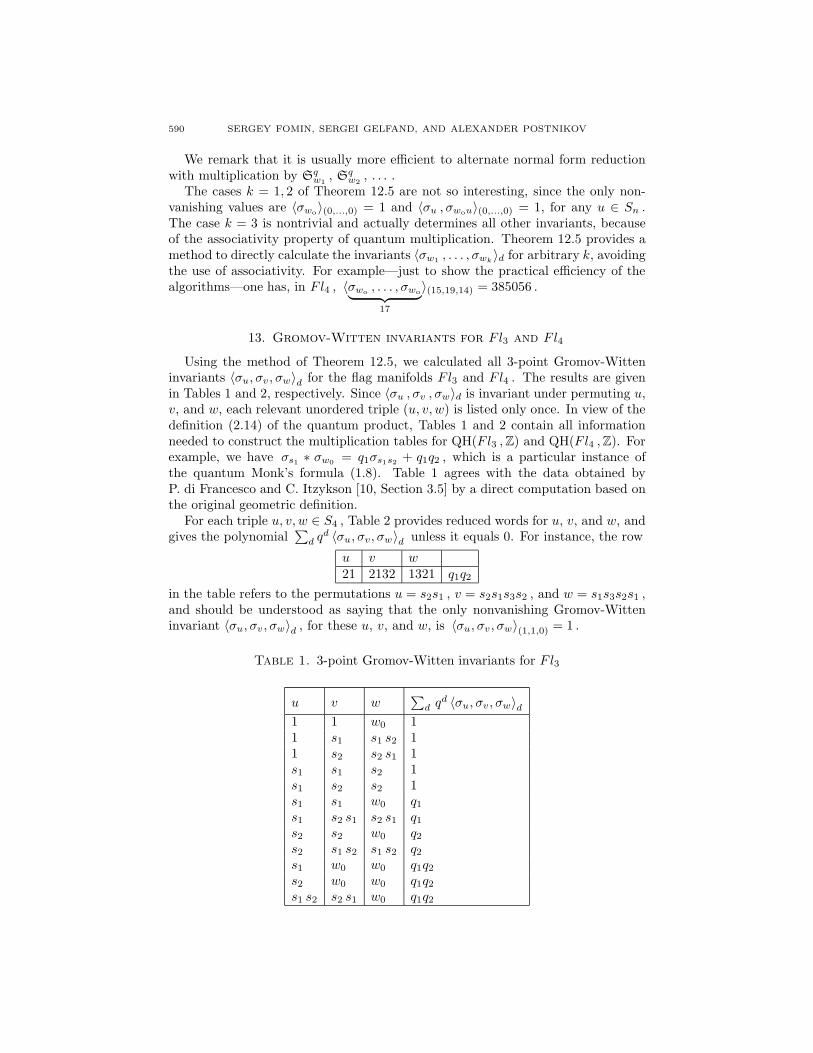
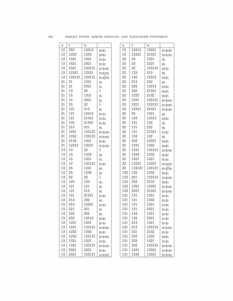
Using the method of Theorem 12.5, we calculated all 3-point Gromov-Witteninvariants 〈σu, σv, σw〉d for the flag manifolds Fl3 and Fl4 . The results are givenin Tables 1 and 2, respectively. Since 〈σu , σv , σw〉d is invariant under permuting u,v, and w, each relevant unordered triple (u, v, w) is listed only once. In view of thedefinition (2.14) of the quantum product, Tables 1 and 2 contain all informationneeded to construct the multiplication tables for QH(Fl3 ,Z) and QH(Fl4 ,Z). Forexample, we have σs1 ∗ σw0 = q1σs1s2 + q1q2 , which is a particular instance ofthe quantum Monk’s formula (1.8). Table 1 agrees with the data obtained byP. di Francesco and C. Itzykson [10, Section 3.5] by a direct computation based onthe original geometric definition.
For each triple u, v, w ∈ S4 , Table 2 provides reduced words for u, v, and w, andgives the polynomial
∑d q
d 〈σu, σv, σw〉d unless it equals 0. For instance, the row
u v w21 2132 1321 q1q2
in the table refers to the permutations u = s2s1 , v = s2s1s3s2 , and w = s1s3s2s1 ,and should be understood as saying that the only nonvanishing Gromov-Witteninvariant 〈σu, σv, σw〉d , for these u, v, and w, is 〈σu, σv, σw〉(1,1,0) = 1 .
Table 1. 3-point Gromov-Witten invariants for Fl3
u v w∑
d qd 〈σu, σv, σw〉d
1 1 w0 11 s1 s1 s2 11 s2 s2 s1 1s1 s1 s2 1s1 s2 s2 1s1 s1 w0 q1s1 s2 s1 s2 s1 q1s2 s2 w0 q2s2 s1 s2 s1 s2 q2s1 w0 w0 q1q2s2 w0 w0 q1q2s1 s2 s2 s1 w0 q1q2

QUANTUM SCHUBERT POLYNOMIALS 591
Table 2. 3-point Gromov-Witten invariants for Fl4
u v wφ φ 123121 1φ 1 12312 1φ 2 12321 1φ 3 21321 1φ 12 1231 1φ 21 1232 1φ 13 2132 1φ 23 1321 1φ 32 2321 1φ 123 121 1φ 132 213 1φ 321 232 11 1 1232 11 1 123121 q11 2 1231 11 2 1232 11 3 2132 11 12 123 11 21 232 11 21 12321 q11 13 132 11 13 232 11 13 21321 q11 23 121 11 23 132 11 32 213 11 32 232 11 121 1231 q11 121 123121 q1q21 213 1321 q11 321 2321 q11 1321 21321 q1q21 12321 123121 q1q2q32 2 1231 12 2 2321 12 2 123121 q22 3 1321 12 3 2321 12 12 213 12 12 12312 q22 21 123 12 21 232 12 13 121 12 13 132 1
u v w2 13 213 12 13 232 12 23 121 12 23 321 12 32 213 12 32 21321 q22 121 1232 q22 121 123121 q1q22 132 2132 q22 232 1321 q22 232 123121 q2q32 1232 12312 q2q32 1321 21321 q1q22 12321 123121 q1q2q33 3 1321 13 3 123121 q33 12 121 13 12 213 13 21 132 13 21 232 13 13 121 13 13 132 13 13 12312 q33 23 121 13 23 12321 q33 32 321 13 123 1231 q33 213 1232 q33 232 2321 q33 232 123121 q2q33 1232 12312 q2q33 12321 123121 q1q2q312 12 13 112 12 1232 q212 21 23 112 21 123121 q1q212 13 13 112 13 23 112 32 2132 q212 121 232 q212 121 12321 q1q212 132 132 q212 132 232 q212 321 21321 q1q2
592 SERGEY FOMIN, SERGEI GELFAND, AND ALEXANDER POSTNIKOV
u v w12 232 12312 q2q312 1232 1232 q2q312 1321 1321 q1q212 1321 2321 q1q212 2321 123121 q1q2q312 12321 12321 q1q2q312 123121 123121 q1q
22q3
21 21 1231 q121 21 2321 q121 13 32 121 13 1321 q121 13 2321 q121 23 32 121 121 213 q121 121 12312 q1q221 121 21321 q1q221 132 21321 q1q221 213 321 q121 1231 123121 q1q2q321 1232 123121 q1q2q321 2132 1321 q1q221 12312 12321 q1q2q313 13 32 113 13 1232 q313 13 1321 q113 13 123121 q1q313 23 1231 q313 23 1232 q313 32 32 113 123 123 q313 121 121 q113 121 213 q113 121 21321 q1q213 213 232 q313 213 12321 q1q313 321 321 q113 232 232 q313 232 12312 q2q313 1231 1231 q1q313 1231 123121 q1q2q313 1232 1232 q2q313 1232 123121 q1q2q313 1321 1321 q1q213 1321 123121 q1q2q313 2321 2321 q1q313 2321 123121 q1q2q3
u v w13 12312 12321 q1q2q313 12321 21321 q1q2q323 23 1231 q323 23 2321 q323 32 123121 q2q323 123 213 q323 132 12312 q2q323 213 232 q323 232 12312 q2q323 232 21321 q2q323 1232 2132 q2q323 1321 123121 q1q2q323 2321 123121 q1q2q323 12321 21321 q1q2q332 32 1321 q232 123 12312 q2q332 121 132 q232 121 232 q232 121 21321 q1q232 132 132 q232 232 12321 q2q332 1231 1232 q2q332 1231 123121 q1q2q332 1232 1232 q2q332 1321 1321 q1q232 12321 12321 q1q2q332 123121 123121 q1q
22q3
123 132 1232 q2q3123 321 123121 q1q2q3123 232 2132 q2q3123 1321 12321 q1q2q3123 2321 21321 q1q2q3121 121 1231 q1q2121 121 1232 q1q2121 121 1321 q1q2121 121 2321 q1q2121 132 1321 q1q2121 132 2321 q1q2121 213 1321 q1q2121 213 123121 q1q2q3121 321 2132 q1q2121 232 1232 q2q3121 232 1321 q1q2121 232 123121 q1q2q3121 1231 12321 q1q2q3121 1232 12321 q1q2q3

QUANTUM SCHUBERT POLYNOMIALS 593
u v w121 2321 12312 q1q2q3121 12312 123121 q1q
22q3
132 213 123121 q1q2q3132 321 1321 q1q2132 232 1231 q2q3132 232 1232 q2q3132 1231 12321 q1q2q3132 2321 12321 q1q2q3132 12312 123121 q1q
22q3
132 21321 123121 q1q22q3
213 213 1231 q1q3213 213 2321 q1q3213 213 123121 q1q2q3213 232 1232 q2q3213 232 123121 q1q2q3213 1231 21321 q1q2q3213 1232 21321 q1q2q3213 2132 12321 q1q2q3213 1321 12312 q1q2q3213 2321 12312 q1q2q3321 1231 12312 q1q2q3321 1232 12321 q1q2q3232 232 1231 q2q3
u v w232 232 1232 q2q3232 232 1321 q2q3232 232 2321 q2q3232 1231 21321 q1q2q3232 1321 12321 q1q2q3232 2321 12321 q1q2q3232 21321 123121 q1q
22q3
1231 1231 1321 q1q2q31231 1232 1321 q1q2q31231 2132 2321 q1q2q31232 1321 2321 q1q2q31232 1321 123121 q1q
22q3
1232 2321 2321 q1q2q31232 21321 21321 q1q
22q3
1232 123121 123121 q1q22q
23
2132 2132 123121 q1q22q3
2132 12312 21321 q1q22q3
1321 12312 12312 q1q22q3
1321 123121 123121 q21q22q3
12312 12312 123121 q1q22q
23
21321 21321 123121 q21q22q3
123121 123121 123121 q21q22q
23
14. Tables of quantum Schubert polynomials
n = 2
w red.word Sw Sqw
12 φ e0 121 1 e1 x1
n = 3
w red.word Sw Sqw
123 φ e00 1213 1 e10 x1
132 2 e01 x1 + x2
231 12 e02 x1x2 + q1312 21 e11 − e02 x2
1 − q1321 121 e12 x1(x1x2 + q1)

594 SERGEY FOMIN, SERGEI GELFAND, AND ALEXANDER POSTNIKOV
n = 4
w red.word Sw Sqw
1234 φ e000 12134 1 e100 x1
1324 2 e010 x1 + x2
1243 3 e001 x1 + x2 + x3
2314 12 e020 x1x2 + q13124 21 e110 − e020 x2
1 − q12143 13 e101 x1(x1 + x2 + x3)1342 23 e002 x1x2 + x1x3 + x2x3 + q1 + q21423 32 e011 − e002 x2
1 + x1x2 + x22 − q1 − q2
2341 123 e003 x1x2x3 + q1x3 + q2x1
3214 121 e120 x1(x1x2 + q1)2413 132 e021 − e003 x2
1x2 + x1x22 + q1x1 + q1x2 − q2x1
3142 213 e102 − e003 x21x2 + x2
1x3 + q1x1 − q1x3
4123 321 e111 − e021 x31 − 2q1x1 − q1x2
− e021 + e0031432 232 e012 − e003 x2
1x2 + x21x3 + x1x
22 + x1x2x3 + x2
2x3
+ q1x1 + q1x2 − q1x3 + q2x2
3241 1231 e103 x1(x1x2x3 + q1x3 + q2x1)2431 1232 e013 (x1 + x2)(x1x2x3 + q1x3 + q2x1)3412 2132 e022 − e013 x2
1x22 + 2q1x1x2 − q2x
21 + q21 + q1q2
4213 1321 e121 − e022 x31x2 + q1x
21 − q1x1x2 − q21 − q1q2
+ e013 − e1034132 2321 e112 − e022 − e103 x3
1x2 + x31x3 + q1x
21 − q1x1x2
− 2q1x1x3 − q1x2x3 − q21 − q1q23421 12312 e023 (x1x2 + q1)(x1x2x3 + q1x3 + q2x1)4231 12321 e113 − e023 (x2
1 − q1)(x1x2x3 + q1x3 + q2x1)4312 21321 e122 − e113 x1(x
21x
22 + 2q1x1x2 − q2x
21 + q21 + q1q2)
4321 123121 e123 x1(x1x2 + q1)(x1x2x3 + q1x3 + q2x1)
Acknowledgments
The authors are grateful to Alexander Astashkevich, Alexander Givental, AlainLascoux, and Yuri Manin for stimulating discussions and helpful remarks. Severalinaccuracies in the original version were corrected by the referee. Our special grat-itude goes to William Fulton for thoughtful comments and suggestions, which ledto substantial improvements of the paper.
The preliminary version of this paper appeared as [12].
References
1. A. Astashkevich and V. Sadov, Quantum cohomology of partial flag manifolds Fn1,...,nk ,Comm. Math. Phys. 170 (1995), 503–528. MR 96g:58027
2. I. N. Bernstein, I. M. Gelfand, and S. I. Gelfand, Schubert cells and cohomology of thespace G/P , Russian Math. Surveys 28 (1973), 1–26. MR 55:2941

QUANTUM SCHUBERT POLYNOMIALS 595
3. A. Bertram, Quantum Schubert calculus, Advances in Math. (to appear).4. S. C. Billey and M. Haiman, Schubert polynomials for the classical groups, J. Amer. Math.
Soc. 8 (1995), 443–482. CMP 95:055. A. Borel, Sur la cohomologie des espaces fibres principaux et des espaces homogenes des
groupes de Lie compacts, Ann. of Math. (2) 57 (1953), 115–207. MR 14:490e6. C. Chevalley, Sur les decompositions cellulaires des espaces G/B, in: Algebraic Groups and
Their Generalizations (W. Haboush and B. Parshall, eds.), Proc. Symp. Pure Math., vol. 56,Part 1, Amer. Math. Soc., Providence, RI, 1994, pp. 1–23. MR 95e:14041
7. I. Ciocan-Fontanine, Quantum cohomology of flag varieties, Intern. Math. Research Notices(1995), no. 6, 263–277. MR 96h:14071
8. M. Demazure, Desingularization des varietes de Schubert generalisees, Ann. Scient. EcoleNormale Sup. (4) 7 (1974), 53–88. MR 50:7174
9. C. Ehresmann, Sur la topologie de certains espaces homogenes, Ann. of Math. 35 (1934),396–443.
10. P. di Francesco and C. Itzykson, Quantum intersection rings, in: The Moduli Space of Curves(R. Dijkgraaf, C. Faber, and G. van der Geer, eds.), Progress in Mathematics, vol. 129,Birkhauser, Boston, 1995, pp. 81–148. MR 96k:14041
11. S. Fomin and A. N. Kirillov, Combinatorial Bn-analogues of Schubert polynomials, Trans.Amer. Math. Soc. 348 (1996), no. 9, 3591–3620. CMP 96:15
12. S. Fomin, S. Gelfand, and A. Postnikov, Quantum Schubert polynomials, AMS electronicpreprint AMSPPS #199605-14-008, April 1996.
13. W. Fulton, Young tableaux with applications to representation theory and geometry, Cam-bridge University Press, 1996.
14. W. Fulton and R. Pandharipande, Notes on stable maps and quantum cohomology, preprintalg-geom/9608011.
15. A. Givental and B. Kim, Quantum cohomology of flag manifolds and Toda lattices, Comm.Math. Phys. 168 (1995), 609–641. MR 96c:58027
16. B. Kim, Quantum cohomology of partial flag manifolds and a residue formula for their in-tersection pairing, Intern. Math. Research Notices (1995), no. 1, 1–16. MR 96c:58028
17. B. Kim, On equivariant quantum cohomology, Intern. Math. Research Notices (1996), no. 17,841–851. CMP 97:04
18. B. Kim, Quantum cohomology of flag manifolds G/B and quantum Toda lattices, preprintalg-geom/9607001.
19. M. Kontsevich and Yu. Manin, Gromov-Witten classes, quantum cohomology, and enumera-tive geometry, Comm. Math. Phys. 164 (1994), 525–562. MR 95i:14049
20. B. Kostant, Flag manifold quantum cohomology, the Toda lattice, and the representation withhighest weight ρ, Selecta Math. (N.S.) 2 (1996), 43–91. CMP 96:16
21. A. Lascoux, Classes de Chern des varietes de drapeaux, C. R. Acad. Sci. Paris 295 (1982),393–398. MR 85e:14074
22. A. Lascoux and M. P. Schutzenberger, Polynomes de Schubert, C. R. Acad. Sci. Paris 294(1982), 447–450. MR 83e:14039
23. A. Lascoux and M. P. Schutzenberger, Fonctorialite de polynomes de Schubert, Contemp.Math. 88 (1989), 585–598. MR 90i:16003
24. J. Li and G. Tian, The quantum cohomology of homogeneous varieties, J. Algebraic Geom.(to appear).
25. I. G. Macdonald, Notes on Schubert polynomials, Publications LACIM, Montreal, 1991.26. D. Monk, The geometry of flag manifolds, Proc. London Math. Soc. 9 (1959), 253–286. MR
21:564127. P. Pragacz and J. Ratajski, Formulas for Lagrangian and orthogonal degeneracy loci; the
Q-polynomial approach, Compositio Math. (to appear).28. Y. Ruan and G. Tian, Mathematical theory of quantum cohomology, J. Diff. Geom. 42 (1995),
no. 2, 259–367. MR 96m:5803329. B. Sturmfels, Algorithms in invariant theory, Springer-Verlag, Berlin, 1993. MR 94m:1300430. C. Vafa, Topological mirrors and quantum rings, in: Essays on Mirror Manifolds (S.-T. Yau,
ed.), International Press, Boston, 1992. MR 94c:8119331. E. Witten, Two-dimensional gravity and intersection theory on moduli space, Surveys in
Differential Geometry, vol. 1, International Press, Boston, 1991, pp. 243–310. MR 93e:32028

596 SERGEY FOMIN, SERGEI GELFAND, AND ALEXANDER POSTNIKOV
Department of Mathematics, Massachusetts Institute of Technology, Cambridge,
Massachusetts 02139
E-mail address: [email protected]
American Mathematical Society, P.O.Box 6248, Providence, Rhode Island 02940-6248
E-mail address: [email protected]
Department of Mathematics, Massachusetts Institute of Technology, Cambridge,
Massachusetts 02139
E-mail address: [email protected]
![SCHUBERT POLYNOMIALS AND DEGENERACY LOCUS FORMULASharryt/papers/spdlf.pdf · SCHUBERT POLYNOMIALS AND DEGENERACY LOCUS FORMULAS 3 in Kazarian’s paper [Ka]. The proof continues by](https://static.fdocuments.us/doc/165x107/5f039a2a7e708231d409dccf/schubert-polynomials-and-degeneracy-locus-formulas-harrytpapersspdlfpdf-schubert.jpg)