Tutorial on Schubert Varieties and Schubert Calculus - icerm

Tutorial on

Schubert Varieties and Schubert Calculus

Sara Billey

University of Washington

http://www.math.washington.edu/∼billey

ICERM TutorialsFebruary 27, 013

Philosophy

“Combinatorics is the equivalent of nanotechnology in mathematics.”

Outline

1. Background and history of Grassmannians

2. Schur functions

3. Background on Flag Manifolds

4. Schubert polynomials

5. The Big Picture

Enumerative Geometry

Approximately 150 years ago. . . Grassmann, Schubert, Pieri, Giambelli, Severi,and others began the study of enumerative geometry .

Early questions:• What is the dimension of the intersection between two general lines in R2?

• How many lines intersect two given lines and a given point in R3?

• How many lines intersect four given lines in R3 ?

Modern questions:

• How many points are in the intersection of 2,3,4,. . . Schubert varieties ingeneral position?

Schubert Varieties

A Schubert variety is a member of a family of projective varieties which is definedas the closure of some orbit under a group action in a homogeneous spaceG/H.

Typical properties:• They are all Cohen-Macaulay, some are “mildly” singular.

• They have a nice torus action with isolated fixed points.

• This family of varieties and their fixed points are indexed by combinatorialobjects; e.g. partitions, permutations, or Weyl group elements.

Schubert Varieties

“Honey, Where are my Schubert varieties?”

Typical contexts:• The Grassmannian Manifold , G(n, d) = GLn/P .

• The Flag Manifold: Gln/B.

• Symplectic and Orthogonal Homogeneous spaces: Sp2n/B, On/P

• Homogeneous spaces for semisimple Lie Groups: G/P .

• Affine Grassmannians: LG = G(C[z, z−1])/P .

More exotic forms: matrix Schubert varieties, Richardson varieties, sphericalvarieties, Hessenberg varieties, Goresky-MacPherson-Kottwitz spaces, positroids.

Why Study Schubert Varieties?

1. It can be useful to see points, lines, planes etc as families with certainproperties.

2. Schubert varieties provide interesting examples for test cases and futureresearch in algebraic geometry, combinatorics and number theory.

3. Applications in discrete geometry, computer graphics, computer vision,and economics.

The Grassmannian Varieties

Definition. Fix a vector space V over C (or R, Qp,. . . ) with basis B ={e1, . . . , en}. The Grassmannian variety

G(k, n) = {k-dimensional subspaces of V }.

Question.

How can we impose the structure of a variety or a manifold on this set?


Answer. Relate G(k, n) to the k × n matrices of rank k.

U =span〈6e1 + 3e2, 4e1 + 2e3, 9e1 + e3 + e4〉 ∈ G(3, 4)

MU =

6 3 0 04 0 2 09 0 1 1

• U ∈ G(k, n) ⇐⇒ rows of MU are independent vectors in V ⇐⇒some k × k minor of MU is NOT zero.

Plucker Coordinates

• Define fj1,j2,...,jk to be the homogeneous polynomial given by the deter-minant of the matrix

x1,j1 x1,j2 . . . x1,jk

x2,j1 x2,j2 . . . x2,jk...

......

...xkj1 xkj2 . . . xkjk

• G(k, n) is an open set in the Zariski topology on k×n matrices definedas the union over all k-subsets of {1, 2, . . . , n} of the complements ofthe varieties V (fj1,j2,...,jk).

• G(k, n) embeds in P(nk )) by listing out the Plucker coordinates.


Canonical Form. Every subspace in G(k, n) can be represented by aunique k × n matrix in row echelon form.

Example.

U =span〈6e1 + 3e2, 4e1 + 2e3, 9e1 + e3 + e4〉 ∈ G(3, 4)

≈

6 3 0 04 0 2 09 0 1 1

=

3 0 00 2 00 1 1

2 1 0 02 0 1 07 0 0 1

≈〈2e1 + e2, 2e1 + e3, 7e1 + e4〉

Subspaces and Subsets

Example.

U = RowSpan

5 9 h1 0 0 0 0 0 0 05 8 0 9 7 9 h1 0 0 04 6 0 2 6 4 0 3 h1 0

∈ G(3, 10).

position(U) = {3, 7, 9}

Definition.

If U ∈ G(k, n) and MU is the corresponding matrix in canonical form thenthe columns of the leading 1’s of the rows of MU determine a subset of size kin {1, 2, . . . , n} := [n]. There are 0’s to the right of each leading 1 and 0’sabove and below each leading 1. This k-subset determines the position of Uwith respect to the fixed basis.

The Schubert Cell Cj in G(k, n)

Defn. Let j = {j1 < j2 < · · · < jk} ∈ [n]. A Schubert cell is

Cj = {U ∈ G(k, n) | position(U) = {j1, . . . , jk}}

Fact. G(k, n) =⋃

Cj over all k-subsets of [n].

Example. In G(3, 10),

C{3,7,9} =

∗ ∗ h1 0 0 0 0 0 0 0∗ ∗ 0 ∗ ∗ ∗ h1 0 0 0∗ ∗ 0 ∗ ∗ ∗ 0 ∗ h1 0

• Observe, dim(C{3,7,9}) = 2 + 5 + 6 = 13.

• In general, dim(Cj) =∑

ji − i.

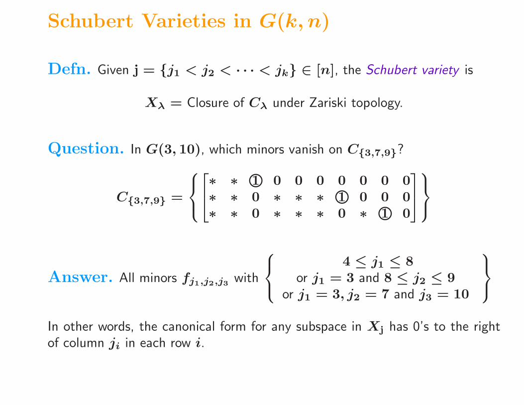
Schubert Varieties in G(k, n)

Defn. Given j = {j1 < j2 < · · · < jk} ∈ [n], the Schubert variety is

Xλ = Closure of Cλ under Zariski topology.

Question. In G(3, 10), which minors vanish on C{3,7,9}?

C{3,7,9} =

∗ ∗ h1 0 0 0 0 0 0 0∗ ∗ 0 ∗ ∗ ∗ h1 0 0 0∗ ∗ 0 ∗ ∗ ∗ 0 ∗ h1 0

Answer. All minors fj1,j2,j3 with

4 ≤ j1 ≤ 8or j1 = 3 and 8 ≤ j2 ≤ 9

or j1 = 3, j2 = 7 and j3 = 10

In other words, the canonical form for any subspace in Xj has 0’s to the rightof column ji in each row i.

k-Subsets and Partitions

Defn. A partition of a number n is a weakly increasing sequence of non-negative integers

λ = (λ1 ≤ λ2 ≤ · · · ≤ λk)

such that n =∑

λi = |λ|.

Partitions can be visualized by their Ferrers diagram

(2, 5, 6) −→

Fact. There is a bijection between k-subsets of {1, 2, . . . , n} and partitionswhose Ferrers diagram is contained in the k × (n − k) rectangle given by

shape : {j1 < . . . < jk} 7→ (j1 − 1, j2 − 2, . . . , jk − k).

A Poset on Partitions

Defn. A partial order or a poset is a reflexive, anti-symmetric, and transitiverelation on a set.

Defn. Young’s LatticeIf λ = (λ1 ≤ λ2 ≤ · · · ≤ λk) and µ = (µ1 ≤ µ2 ≤ · · · ≤ µk) thenλ ⊂ µ if the Ferrers diagram for λ fits inside the Ferrers diagram for µ.

⊂ ⊂

Facts.

1. Xj =⋃

shape(i)⊂shape(j)

Ci.

2. The dimension of Xj is |shape(j)|.

3. The GrassmannianG(k, n) = X{n−k+1,...,n−1,n} is a Schubert variety!

Singularities in Schubert Varieties

Theorem. (Lakshmibai-Weyman) Given a partition λ. The singular locus ofthe Schubert variety Xλ in G(k, n) is the union of Schubert varieties indexedby the set of all partitions µ ⊂ λ obtained by removing a hook from λ.

Example. sing((X(4,3,1)) = X(4) ∪ X(2,2,1)

•• • • •

• •

Corollary. Xλ is non-singular if and only if λ is a rectangle.

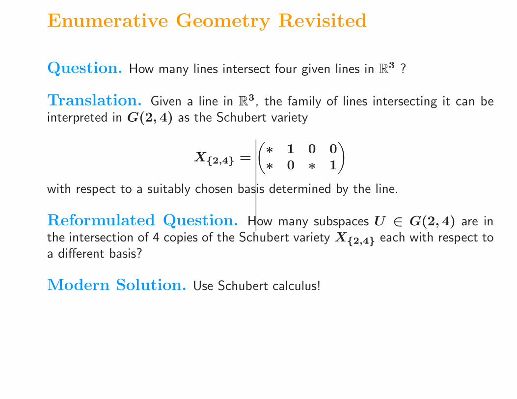
Enumerative Geometry Revisited

Question. How many lines intersect four given lines in R3 ?

Translation. Given a line in R3, the family of lines intersecting it can beinterpreted in G(2, 4) as the Schubert variety

X{2,4} =

(∗ 1 0 0∗ 0 ∗ 1

)

with respect to a suitably chosen basis determined by the line.

Reformulated Question. How many subspaces U ∈ G(2, 4) are inthe intersection of 4 copies of the Schubert variety X{2,4} each with respect toa different basis?

Modern Solution. Use Schubert calculus!

Schubert Calculus/Intersection Theory

• Schubert varieties induce canonical basis elements of the cohomology ringH∗(G(k, n)) called Schubert classes: [Xj].

• Multiplication in H∗(G(k, n)) is determined by intersecting Schubertvarieties with respect to generically chosen bases

[Xi][Xj] =[Xi(B

1) ∩ Xj(B2)]

• The entire multiplication table is determined by

Giambelli Formula: [Xi] = det(eλ′

i−i+j

)1≤i,j≤k

Pieri Formula: [Xi] er =∑

[Xj]

Intersection Theory/Schubert Calculus

• Schubert varieties induce canonical basis elements of the cohomology ringH∗(G(k, n)) called Schubert classes: [Xj].

• Multiplication in H∗(G(k, n)) is determined by intersecting Schubertvarieties with respect to generically chosen bases

[Xi][Xj] =[Xi(B

1) ∩ Xj(B2)]

• The entire multiplication table is determined by

Giambelli Formula: [Xi] = det(eλ′

i−i+j

)1≤i,j≤k

Pieri Formula: [Xi] er =∑

[Xj]

where the sum is over classes indexed by shapes obtained from shape(i)by removing a vertical strip of r cells.

• λ′ = (λ′1, . . . , λ

′k) is the conjugate of the box complement of shape(i).

• er is the special Schubert class associated to k× n minus r boxes alongthe right col. er is a Chern class in the Chern roots x1, . . . , xn.

Intersection Theory/Schubert Calculus

Schur functions Sλ are a fascinating family of symmetric functions indexed bypartitions which appear in many areas of math, physics, theoretical computerscience, quantum computing and economics.

• The Schur functions Sλ are symmetric functions that also satisfy

Giambelli/Jacobi-Trudi Formula: Sλ = det(eλ′

i−i+j

)1≤i,j≤k

Pieri Formula: Sλ er =∑

Sµ.

• Thus, as rings H∗(G(k, n)) ≈ C[x1, . . . , xn]Sn/〈Sλ : λ 6⊂ k × n〉.

• Expanding the product of two Schur functions into the basis of Schurfunctions can be done via linear algebra:

SλSµ =∑

cνλ,µSν .

• The coefficients cνλ,µ are non-negative integers called the Littlewood-Richardson coefficients.

Schur Functions

Let X = {x1, x2, . . . , xn} be an alphabet of indeterminants.

Let λ = (λ1 ≥ λ2 ≥ · · · ≥ λk > 0) and λp = 0 for p ≥ k.

Defn. The following are equivalent definitions for the Schur functions Sλ(X):

1. Sλ = det(eλ′

i−i+j

)= det (hλi−i+j)

2. Sλ =det(x

λj+n−j

i)

det(xn−j

i)

with indices 1 ≤ i, j ≤ m.

3. Sλ =∑

xT summed over all column strict tableaux T of shape λ.

4. Sλ =∑

FD(T )(X) summed over all standard tableaux T of shape λ.

Schur Functions

Defn. Sλ =∑

FD(T )(X) over all standard tableaux T of shape λ.

Defn. A standard tableau T of shape λ is a saturated chain in Young’s latticefrom ∅ to λ. The descent set of T is the set of indices i such that i+1 appearsnorthwest of i.

Example.

T = 74 5 91 2 3 6 8

D(T ) = {3, 6, 8}.

Defn. The fundamental quasisymmetric function

FD(T )(X) =∑

xi1 · · ·xip

summed over all 1 ≤ i1 ≤ . . . ≤ ip such that ij < ij+1 whenever j ∈ D(T ).

Littlewood-Richardson Rules

Recall if SλSµ =∑

cνλ,µSν , then the coefficients cνλ,µ are non-negative inte-gers called Littlewood-Richardson coefficients.

Littlewood-Richardson Rules.1. Schutzenberger: Fix a standard tableau T of shape ν. Then cνλ,µ equals

the number of pairs of standard tableaux of shapes λ, µ which straightenunder the rules of jeu de taquin into T .

2. Yamanouchi Words: cνλ,µ equals the number of column strict fillings ofthe skew shape ν/µ with λ1 1’s, λ2 2’s, etc such that the reverse readingword always has more 1’s than 2’s, more 2’s than 3’s, etc.

3. Remmel-Whitney rule: cνλ,µ equals the number of leaves of shape ν inthe tree of standard tableaux with root given by the standard labeling ofλ and growing on at each level respecting two adjacency rules.

4. Knutson-Tao Puzzles: cνλ,µ equals the number of λ, µ, ν - puzzles.

5. Vakil Degenerations: cνλ,µ equals the number of leaves in the λ, µ-tree ofcheckerboards with type ν.

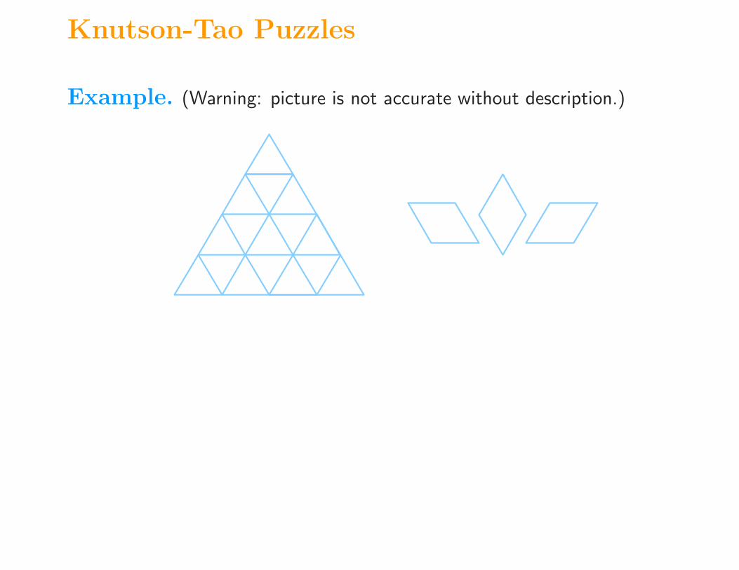
Knutson-Tao Puzzles

Example. (Warning: picture is not accurate without description.)

Vakil Degenerations

Show picture.

Enumerative Solution


Enumerative Solution


Solution. [X{2,4}

]= S(1) = x1 + x2 + . . .

By the recipe, compute

[X{2,4}(B

1) ∩ X{2,4}(B2) ∩ X{2,4}(B

3) ∩ X{2,4}(B4)]

= S4(1) = 2S(2,2) + S(3,1) + S(2,1,1).

Answer. The coefficient of S2,2 = [X1,2] is 2 representing the two linesmeeting 4 given lines in general position.

Recap

1. G(k, n) is the Grassmannian variety of k-dim subspaces in Rn.

2. The Schubert varieties in G(k, n) are nice projective varieties indexed byk-subsets of [n] or equivalently by partitions in the k×(n−k) rectangle.

3. Geometrical information about a Schubert variety can be determined bythe combinatorics of partitions.

4. Schubert Calculus (intersection theory applied to Schubert varieties andassociated algorithms for Schur functions) can be used to solve problemsin enumerative geometry.

Current Research

1. (Gelfand-Goresky-MacPherson-Serganova) Matroid stratification ofG(k, n):specify the complete list of Plucker coordinates which are non-zero. Whatis the cohomology class of the closure of each strata?

2. (Kodama-Williams, Telaska-Williams) Deodhar stratification using Go-diagrams. What is the cohomology class of the closure of each strata?

3. (MacPherson) What is a good way to triangulate Gr(k,n)?

The Flag Manifold

Defn. A complete flag F• = (F1, . . . , Fn) in Cn is a nested sequence ofvector spaces such that dim(Fi) = i for 1 ≤ i ≤ n. F• is determined by anordered basis 〈f1, f2, . . . fn〉 where Fi = span〈f1, . . . , fi〉.

Example.

F• =〈6e1 + 3e2, 4e1 + 2e3, 9e1 + e3 + e4, e2〉

��

��

��

��

��

��

��

��

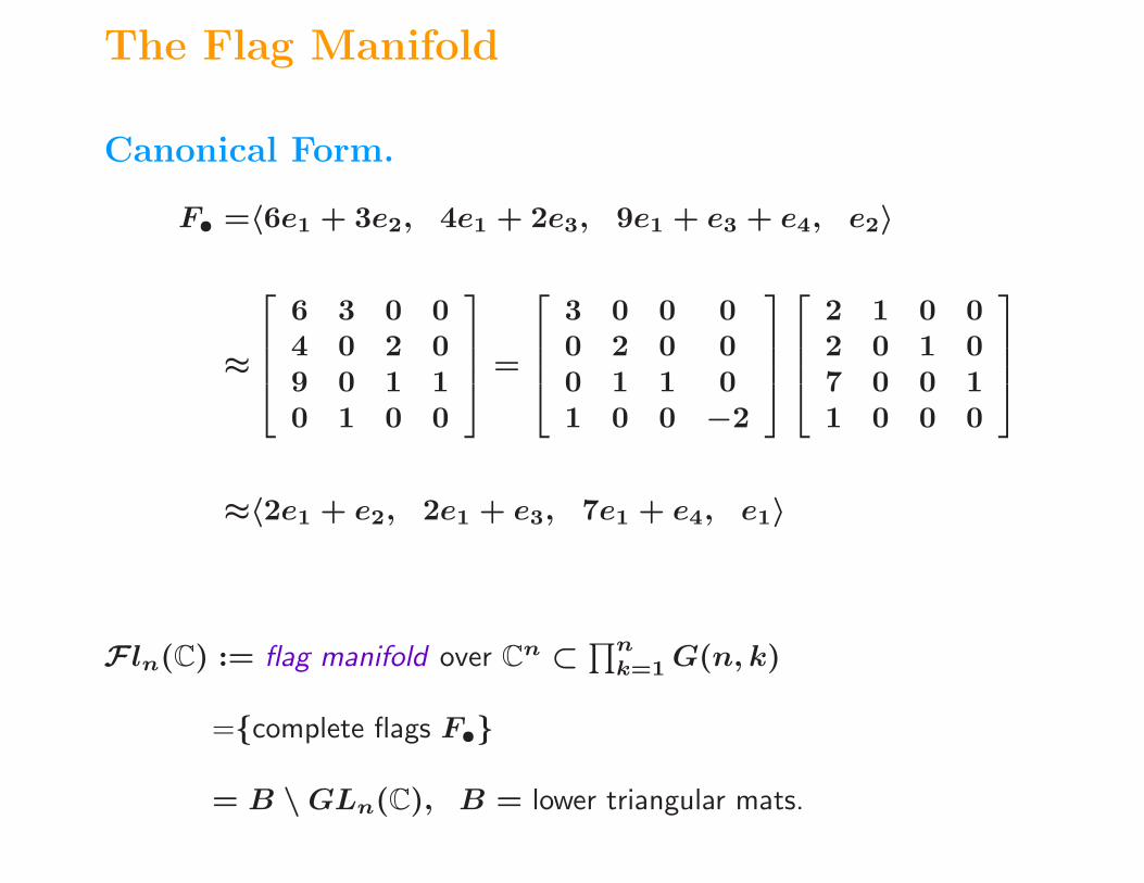
The Flag Manifold

Canonical Form.

F• =〈6e1 + 3e2, 4e1 + 2e3, 9e1 + e3 + e4, e2〉

≈

6 3 0 04 0 2 09 0 1 10 1 0 0

=

3 0 0 00 2 0 00 1 1 01 0 0 −2

2 1 0 02 0 1 07 0 0 11 0 0 0

≈〈2e1 + e2, 2e1 + e3, 7e1 + e4, e1〉

Fln(C) := flag manifold over Cn ⊂∏n

k=1 G(n, k)

={complete flags F•}

= B \ GLn(C), B = lower triangular mats.

Flags and Permutations

Example. F• = 〈2e1+e2, 2e1+e3, 7e1+e4, e1〉 ≈

2 h1 0 02 0 h1 07 0 0 h1h1 0 0 0

Note. If a flag is written in canonical form, the positions of the leading 1’sform a permutation matrix. There are 0’s to the right and below each leading1. This permutation determines the position of the flag F• with respect to thereference flag E• = 〈e1, e2, e3, e4 〉.

��

��

��

��

��

��

��

��

��

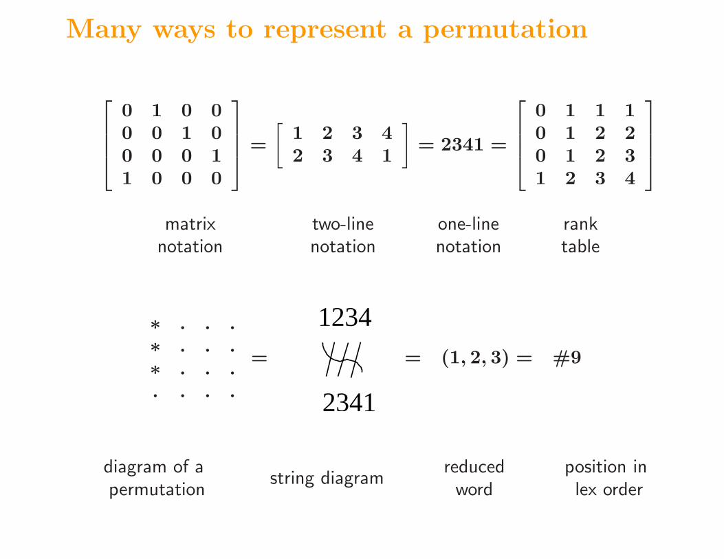
Many ways to represent a permutation

0 1 0 00 0 1 00 0 0 11 0 0 0

=

[1 2 3 42 3 4 1

]= 2341 =

0 1 1 10 1 2 20 1 2 31 2 3 4

matrixnotation

two-linenotation

one-linenotation

ranktable

∗ . . .∗ . . .∗ . . .. . . .

= = (1, 2, 3) = #9

1234

2341

diagram of apermutation

string diagramreducedword

position inlex order

The Schubert Cell Cw(E•) in Fln(C)

Defn. Cw(E•) = All flags F• with position(E•, F•) = w

= {F• ∈ Fln | dim(Ei ∩ Fj) = rk(w[i, j])}

Example. F• =

2 h1 0 02 0 h1 07 0 0 h1h1 0 0 0

∈ C2341 =

∗ 1 0 0∗ 0 1 0∗ 0 0 11 0 0 0

: ∗ ∈ C

Easy Observations.• dimC(Cw) = l(w) = # inversions of w.

• Cw = w · B is a B-orbit using the right B action, e.g.

0 1 0 0

0 0 1 0

0 0 0 1

1 0 0 0

b1,1 0 0 0

b2,1 b2,2 0 0

b3,1 b3,2 b3,3 0

b4,1 b4,2 b4,3 b4,4

=

b2,1 b2,2 0 0

b3,1 b3,2 b3,3 0

b4,1 b4,2 b4,3 b4,4

b1,1 0 0 0

The Schubert Variety Xw(E•) in Fln(C)

Defn. Xw(E•) = Closure of Cw(E•) under the Zariski topology

= {F• ∈ Fln | dim(Ei ∩ Fj)≥rk(w[i, j])}

where E• = 〈e1, e2, e3, e4 〉.

Example.

h1 0 0 00 ∗ h1 00 ∗ 0 h10 h1 0 0

∈ X2341(E•) =

∗ 1 0 0∗ 0 1 0∗ 0 0 11 0 0 0

Why?.

��

��

��

��

��

��

��

��

��

��

��

��

��

��

��

��

��

��

��

��

Five Fun Facts

Fact 1. The closure relation on Schubert varieties defines a nice partial order.

Xw =⋃

v≤w

Cv =⋃

v≤w

Xv

Bruhat order (Ehresmann 1934, Chevalley 1958) is the transitive closure of

w < wtij ⇐⇒ w(i) < w(j).

Example. Bruhat order on permutations in S3.

132

231

123

321

213

312

��

@@��

@@ ��

@@@

Observations. Self dual, rank symmetric, rank unimodal.

Bruhat order on S4

4 2 3 1

3 1 2 4

4 2 1 3

1 2 3 4

3 4 2 1

1 2 4 3

3 2 1 4

2 1 3 4

2 3 1 4

3 2 4 12 4 3 1

2 3 4 1 4 1 2 3

4 1 3 2

1 4 2 3

1 4 3 2

4 3 1 2

3 1 4 2

1 3 4 2

3 4 1 2

2 1 4 3

1 3 2 4

2 4 1 3

4 3 2 1

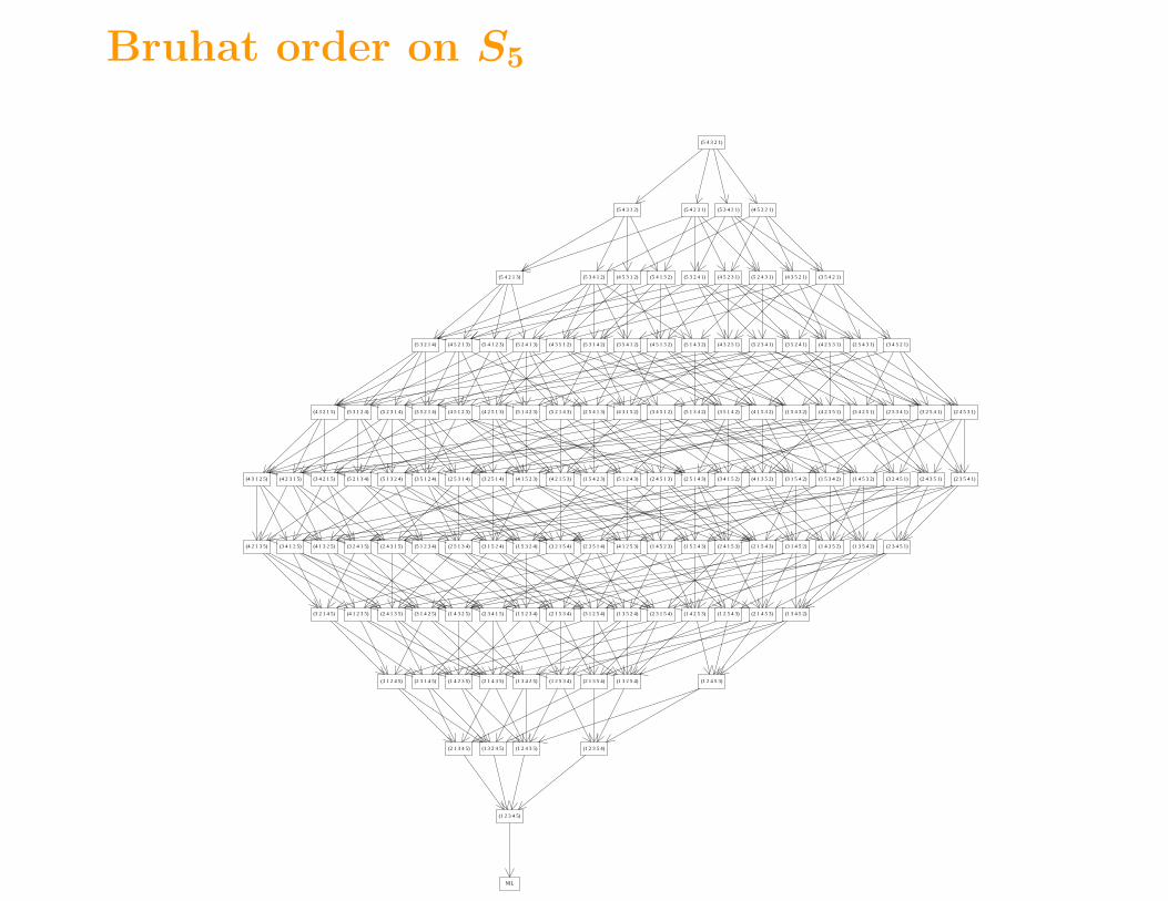
Bruhat order on S5

(3 4 2 1 5)

(2 4 1 5 3)

(3 4 2 5 1)

(4 5 3 1 2)

(4 1 3 5 2)

(2 3 4 1 5)

(3 4 1 2 5)

(4 2 1 5 3)

(3 5 4 1 2)

(1 5 3 2 4) (2 3 4 5 1)

(5 3 4 1 2)

(5 1 3 2 4)

(2 4 5 3 1)

(4 1 3 2 5)

(2 1 4 3 5)

(2 5 3 1 4)

(5 4 1 2 3)

(5 2 1 3 4)

(2 5 4 1 3)

(3 5 4 2 1)

(5 1 4 3 2)

(1 3 4 2 5)

(5 4 1 3 2)

(1 5 4 2 3)

(3 1 4 2 5)

(5 4 2 3 1) (4 5 3 2 1)

(1 4 2 3 5)

(5 3 4 2 1)

(1 2 3 5 4)

(2 5 4 3 1)

(1 3 5 4 2)

(1 2 4 5 3)

(2 1 5 4 3)

(3 1 5 4 2) (2 4 3 5 1)

(5 2 3 4 1)

(1 4 3 5 2)

(2 3 5 4 1)

(2 4 3 1 5)

(3 2 4 5 1)

(5 1 4 2 3)

(5 4 3 1 2)

(2 4 1 3 5)

(1 5 4 3 2)

(2 3 5 1 4)(4 2 1 3 5)

(4 2 3 5 1)

(4 2 3 1 5)

(5 4 2 1 3)

(1 2 3 4 5)

(4 1 5 2 3)

(5 2 3 1 4)

(3 2 4 1 5)

(1 2 4 3 5)

(5 2 4 1 3) (4 3 5 1 2)

(5 4 3 2 1)

(2 1 5 3 4)(1 4 3 2 5)

(4 1 5 3 2)

(5 2 4 3 1)

(1 3 5 2 4)

(2 3 1 4 5)

(1 2 5 4 3)

(3 1 5 2 4)

(5 3 1 4 2)

(1 5 2 4 3)

(4 3 5 2 1)

(3 5 2 4 1)

(5 1 2 4 3)

(1 3 2 4 5)

(2 3 1 5 4)

(3 2 5 1 4)

(3 1 2 4 5)

(4 1 2 5 3)

(5 3 2 1 4)

(2 5 1 4 3)

(5 3 2 4 1)

(3 5 2 1 4)

(1 3 2 5 4)

(3 5 1 4 2)

(1 4 5 2 3)

(3 1 2 5 4)

(3 2 5 4 1)

(3 5 1 2 4)

(4 3 2 5 1)

(4 3 2 1 5) (5 3 1 2 4) (4 3 1 5 2) (3 4 5 1 2)

(1 4 5 3 2)(2 4 5 1 3)

(3 4 5 2 1)

(4 1 2 3 5)

(4 5 2 1 3)

(4 3 1 2 5)

(3 2 1 4 5)

(4 2 5 1 3)

(2 5 1 3 4)

(2 5 3 4 1)(4 5 1 2 3) (5 2 1 4 3)

(1 4 2 5 3)

(1 2 5 3 4)

(1 5 3 4 2)

(1 3 4 5 2)(1 5 2 3 4)

(2 1 3 4 5)

(3 1 4 5 2)(5 1 2 3 4)

(2 1 3 5 4)

(3 2 1 5 4)

(4 5 1 3 2)

(2 1 4 5 3)

NIL

(4 5 2 3 1)

(3 4 1 5 2)

(4 2 5 3 1)

(5 1 3 4 2)

10 Fantastic Facts on Bruhat Order

1. Bruhat Order Characterizes Inclusions of Schubert Varieties

2. Contains Young’s Lattice in S∞

3. Nicest Possible Mobius Function

4. Beautiful Rank Generating Functions

5. [x, y] Determines the Composition Series for Verma Modules

6. Symmetric Interval [0, w] ⇐⇒ X(w) rationally smooth

7. Order Complex of (u, v) is shellable

8. Rank Symmetric, Rank Unimodal and k-Sperner

9. Efficient Methods for Comparison

10. Amenable to Pattern Avoidance


Defn. Xw is singular at a point p ⇐⇒dimXw = l(w) < dimension of the tangent space to Xw at p.

Observation 1. Every point on a Schubert cell Cv in Xw looks locally thesame. Therefore, p ∈ Cv is a singular point ⇐⇒ the permutation matrix vis a singular point of Xw.

Observation 2. The singular set of a varieties is a closed set in the Zariskitopology. Therefore, if v is a singular point in Xw then every point in Xv issingular. The irreducible components of the singular locus of Xw is a union ofSchubert varieties:

Sing(Xw) =⋃

v∈maxsing(w)

Xv.


Fact 2. (Lakshmibai-Seshadri) A basis for the tangent space to Xw at v isindexed by the transpositions tij such that

vtij ≤ w.

Definitions.• Let T = invertible diagonal matrices. The T -fixed points in Xw are thepermutation matrices indexed by v ≤ w.

• If v, vtij are permutations in Xw they are connected by a T -stable curve.The set of all T -stable curves in Xw are represented by the Bruhat graphon [id, w].

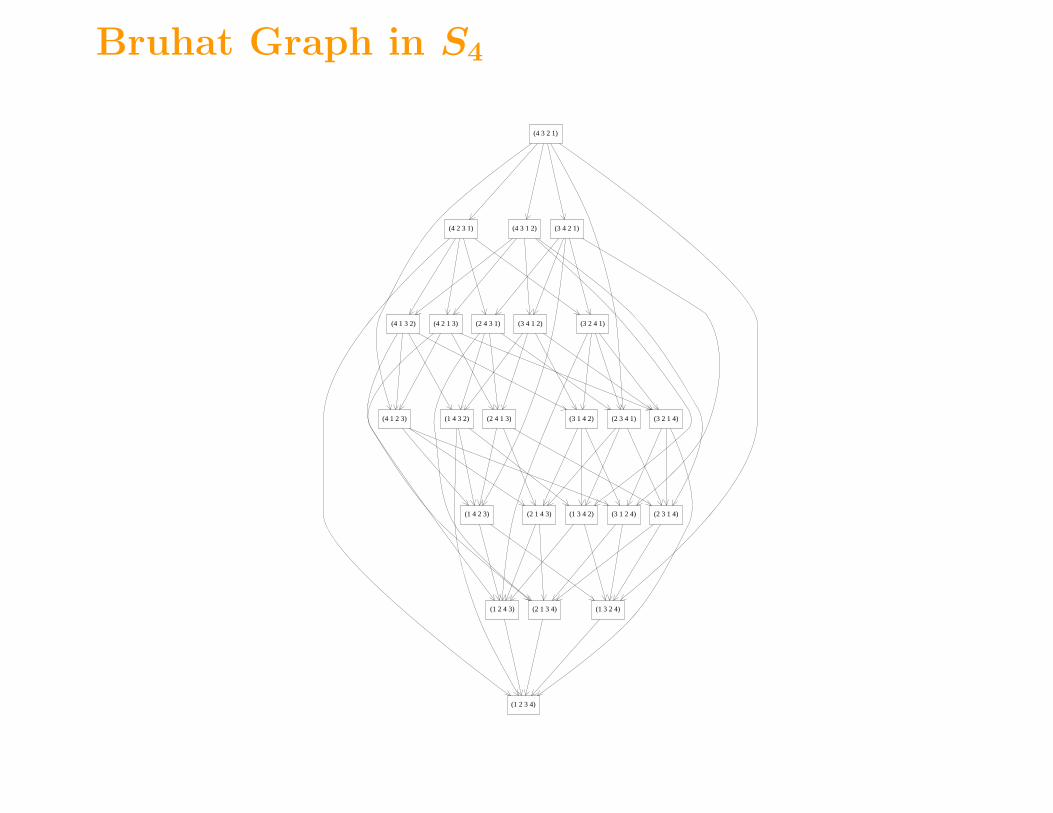
Bruhat Graph in S4

(2 3 4 1)(2 4 1 3)

(1 2 3 4)

(1 3 4 2)(1 4 2 3)

(3 2 4 1)(2 4 3 1)

(2 1 3 4)

(4 2 1 3)

(1 4 3 2) (3 1 4 2) (3 2 1 4)

(2 3 1 4)

(4 1 2 3)

(1 3 2 4)

(3 1 2 4)

(3 4 1 2)

(4 2 3 1) (3 4 2 1)

(2 1 4 3)

(1 2 4 3)

(4 3 1 2)

(4 1 3 2)

(4 3 2 1)

Tangent space of a Schubert Variety

Example. T1234(X4231) = span{xi,j | tij ≤ w}.

(4 2 3 1)

(2 1 3 4)

(1 2 3 4)

(2 4 3 1)

(3 2 1 4)

(4 1 3 2)(3 2 4 1)

(1 4 3 2)(4 1 2 3)(3 1 4 2)

(1 4 2 3)

(1 3 2 4)

(1 3 4 2)

(4 2 1 3)

(2 1 4 3)

(1 2 4 3)

(2 4 1 3)

(2 3 1 4)(3 1 2 4)

(2 3 4 1)

dimX(4231)=5 dimTid(4231) = 6 =⇒ X(4231) is singular!

Five Fun Facts

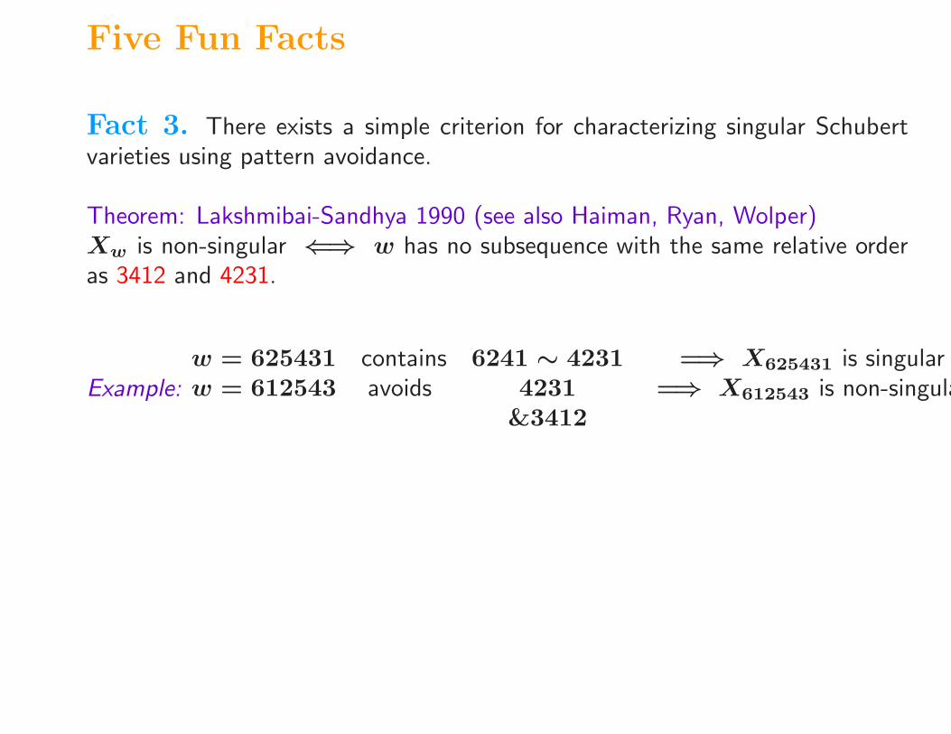
Fact 3. There exists a simple criterion for characterizing singular Schubertvarieties using pattern avoidance.

Theorem: Lakshmibai-Sandhya 1990 (see also Haiman, Ryan, Wolper)Xw is non-singular ⇐⇒ w has no subsequence with the same relative orderas 3412 and 4231.

Example:w = 625431 contains 6241 ∼ 4231 =⇒ X625431 is singularw = 612543 avoids 4231 =⇒ X612543 is non-singula

&3412

Five Fun Facts

Fact 4. There exists a simple criterion for characterizing Gorenstein Schubertvarieties using modified pattern avoidance.

Theorem: Woo-Yong (Sept. 2004)

Xw is Gorenstein ⇐⇒

• w avoids 31542 and 24153 with Bruhat restrictions {t15, t23} and{t15, t34}

• for each descent d in w, the associated partition λd(w) has all of its innercorners on the same antidiagonal.

See “A Unification Of Permutation Patterns Related To Schubert Varieties” byHenning Ulfarsson (arxiv 2012).

Five Fun Facts

Fact 5. Schubert varieties are useful for studying the cohomology ring of theflag manifold.

Theorem (Borel): H∗(Fln) ∼=Z[x1, . . . , xn]

〈e1, . . . en〉.

• The symmetric function ei =∑

1≤k1<···<ki≤n

xk1xk2

. . . xki.

• {[Xw] | w ∈ Sn} form a basis for H∗(Fln) over Z.

Question. What is the product of two basis elements?

[Xu] · [Xv] =∑

[Xw]cwuv.

Cup Product in H∗(Fln)

One Answer. Use Schubert polynomials! Due to Lascoux-Schutzenberger,Bernstein-Gelfand-Gelfand, Demazure.

• BGG: Set [Xid] ≡∏

i>j

(xi − xj) ∈Z[x1, . . . , xn]

〈e1, . . . en〉

If Sw ≡ [Xw]mod〈e1, . . . en〉 then

∂iSw =Sw − siSw

xi − xi+1

≡ [Xwsi] if l(w) < l(wsi)

• LS: Choosing [Xid] ≡ xn−11 xn−2

2 · · ·xn−1 works best because productexpansion can be done without regard to the ideal!

• Here deg[Xw] = codim(Xw).

Schubert polynomials for S4

Sw0(1234) = 1Sw0(2134) = x1

Sw0(1324) = x2 + x1

Sw0(3124) = x21

Sw0(2314) = x1x2

Sw0(3214) = x21x2

Sw0(1243) = x3 + x2 + x1

Sw0(2143) = x1x3 + x1x2 + x21

Sw0(1423) = x22 + x1x2 + x2

1

Sw0(4123) = x31

Sw0(2413) = x1x22 + x2

1x2

Sw0(4213) = x31x2

Sw0(1342) = x2x3 + x1x3 + x1x2

Sw0(3142) = x21x3 + x2

1x2

Sw0(1432) = x22x3 + x1x2x3 + x2

1x3 + x1x22 + x2

1x2

Sw0(4132) = x31x3 + x3

1x2

Sw0(3412) = x21x

22

Sw0(4312) = x31x

22

Sw0(2341) = x1x2x3

Sw0(3241) = x21x2x3

Sw0(2431) = x1x22x3 + x2

1x2x33


Key Feature. Schubert polynomials are a positive sum of monomials andhave distinct leading terms, therefore expanding any polynomial in the basis ofSchubert polynomials can be done by linear algebra just like Schur functions.

Buch: Fastest approach to multiplying Schubert polynomials uses Lascoux andSchutzenberger’s transition equations. Works up to about n = 15.

Draw Back. Schubert polynomials don’t prove cwuv’s are nonnegative (ex-cept in special cases).


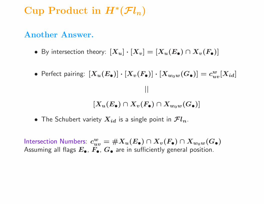
Another Answer.

• By intersection theory: [Xu] · [Xv] = [Xu(E•) ∩ Xv(F•)]

• Perfect pairing: [Xu(E•)] · [Xv(F•)] · [Xw0w(G•)] = cwuv[Xid]

||

[Xu(E•) ∩ Xv(F•) ∩ Xw0w(G•)]

• The Schubert variety Xid is a single point in Fln.

Intersection Numbers: cwuv = #Xu(E•) ∩ Xv(F•) ∩ Xw0w(G•)Assuming all flags E•, F•, G• are in sufficiently general position.

Intersecting Schubert Varieties

Example. Fix three flags R•, G•, and B•:

��

��

��

Find Xu(R•)∩Xv(G•) ∩Xw(B•) where u, v, w are the following permu-tations:

R1 R2 R3 G1 G2 G3 B1 B2 B3

P 1

P 2

P 3

11

1

11

1

11

1



��

��

��

��


R1 R2 R3 G1 G2 G3 B1 B2 B3

P 1

P 2

P 3

11

1

11

1

11

1



��

��

��


R1 R2 R3 G1 G2 G3 B1 B2 B3

P 1

P 2

P 3

11

1

11

1

11

1


Schubert’s Problem. How many points are there usually in the inter-section of d Schubert varieties if the intersection is 0-dimensional?

• Solving approx. nd equations with

(n2

)variables is challenging!

Observation. We need more information on spans and intersections of flagcomponents, e.g. dim(E1

x1∩ E2

x2∩ · · · ∩ Ed

xd).

Permutation Arrays

Theorem. (Eriksson-Linusson, 2000) For every set of d flagsE1• , E

2• , . . . , E

d• ,

there exists a unique permutation array P ⊂ [n]d such that

dim(E1x1

∩ E2x2

∩ · · · ∩ Edxd

) = rkP [x].

��

��

R1 R2 R3 R1 R2 R3 R1 R2 R3

B1

B2

B3 h1 1 1

h11 1 2

h1h1 2

1 2 3

G1 G2 G3

Totally Rankable Arrays

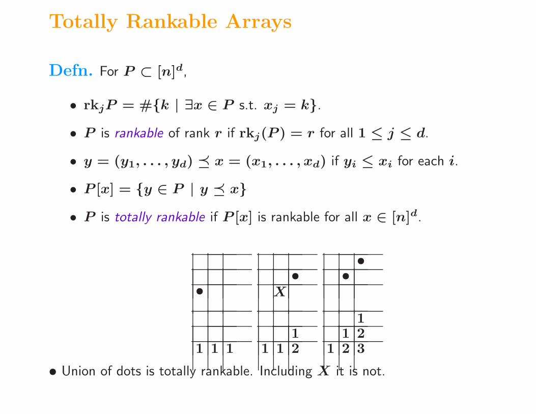
Defn. For P ⊂ [n]d,

• rkjP = #{k | ∃x ∈ P s.t. xj = k}.

• P is rankable of rank r if rkj(P ) = r for all 1 ≤ j ≤ d.

• y = (y1, . . . , yd) � x = (x1, . . . , xd) if yi ≤ xi for each i.

• P [x] = {y ∈ P | y � x}

• P is totally rankable if P [x] is rankable for all x ∈ [n]d.

••

X

••

1 1 11

1 1 2

11 2

1 2 3

• Union of dots is totally rankable. Including X it is not.

Permutation Arrays

••

•• OO

1 1 11

1 1 2

11 2

1 2 3

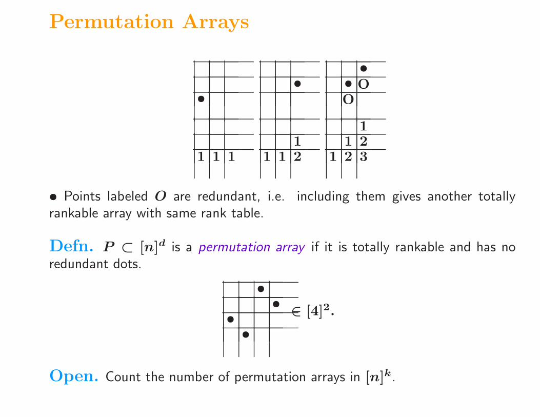
• Points labeled O are redundant, i.e. including them gives another totallyrankable array with same rank table.

Defn. P ⊂ [n]d is a permutation array if it is totally rankable and has noredundant dots.

••

••

∈ [4]2.

Open. Count the number of permutation arrays in [n]k.

Permutation Arrays

Theorem. (Eriksson-Linusson) Every permutation array in [n]d+1 can beobtained from a unique permutation array in [n]d by identifying a sequence ofantichains.

sh

sh

sh

•sh

•

shsh

••

This produces the 3-dimensional array

P = {(4, 4, 1), (2, 4, 2), (4, 2, 2), (3, 1, 3), (1, 4, 4), (2, 3, 4)}.

44 2

32 1

Unique Permutation Array Theorem

Theorem.(Billey-Vakil, 2005) If

X = Xw1(E1•) ∩ · · · ∩ Xwd(Ed

•)

is nonempty 0-dimensional intersection of d Schubert varieties with respect toflags E1

• , E2• , . . . , E

d• in general position, then there exists a unique permuta-

tion array P ∈ [n]d+1 such that

X = {F• | dim(E1x1

∩ E2x2

∩ · · · ∩ Edxd

∩ Fxd+1) = rkP [x].} (1)

Furthermore, we can recursively solve a family of equations for X using P .

Current Research

Open Problem. Can one find a finite set of rules for moving dots in a 3-dpermutation array which determines the cwuv’s analogous to one of the manyLittlewood-Richardson rules?

Recent Progress/Open question. Izzet Coskun’s Mondrian tableaux.Can his algorithm be formulated succinctly enough to program without solvingequations?

Open Problem. Give a minimal list of relations for H∗(Xw). (See recentwork of Reiner-Woo-Yong.)

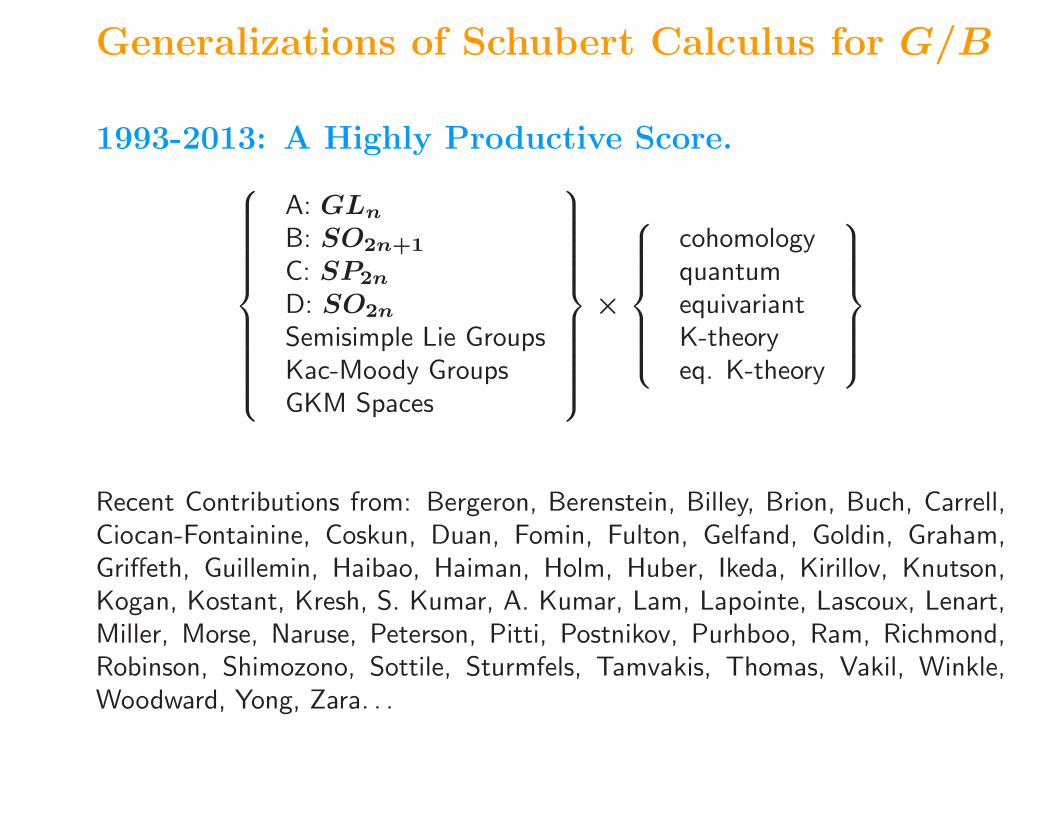
Generalizations of Schubert Calculus for G/B

1993-2013: A Highly Productive Score.

A: GLn

B: SO2n+1

C: SP2n

D: SO2n

Semisimple Lie GroupsKac-Moody GroupsGKM Spaces

×

cohomologyquantumequivariantK-theoryeq. K-theory

Recent Contributions from: Bergeron, Berenstein, Billey, Brion, Buch, Carrell,Ciocan-Fontainine, Coskun, Duan, Fomin, Fulton, Gelfand, Goldin, Graham,Griffeth, Guillemin, Haibao, Haiman, Holm, Huber, Ikeda, Kirillov, Knutson,Kogan, Kostant, Kresh, S. Kumar, A. Kumar, Lam, Lapointe, Lascoux, Lenart,Miller, Morse, Naruse, Peterson, Pitti, Postnikov, Purhboo, Ram, Richmond,Robinson, Shimozono, Sottile, Sturmfels, Tamvakis, Thomas, Vakil, Winkle,Woodward, Yong, Zara. . .

Some Recommended Further Reading

1. “Schubert Calculus” by Steve Kleiman and Dan Laksov. The AmericanMathematical Monthly, Vol. 79, No. 10. (Dec., 1972), pp. 1061-1082.

2. “The Symmetric Group” by Bruce Sagan, Wadsworth, Inc., 1991.

3. ”Young Tableaux” by William Fulton, London Math. Soc. Stud. Texts,Vol. 35, Cambridge Univ. Press, Cambridge, UK, 1997.

4. “Determining the Lines Through Four Lines” by Michael Hohmeyer andSeth Teller, Journal of Graphics Tools, 4(3):11-22, 1999.

5. “Honeycombs and sums of Hermitian matrices” by Allen Knutson andTerry Tao. Notices of the AMS, February 2001; awarded the Conant prizefor exposition.

Some Recommended Further Reading

6. “A geometric Littlewood-Richardson rule” by Ravi Vakil, Annals of Math.164 (2006), 371-422.

7. “Flag arrangements and triangulations of products of simplices” by SaraBilley and Federico Ardila, Adv. in Math, volume 214 (2007), no. 2,495–524.

8. “A Littlewood-Richardson rule for two-step flag varieties” by Izzet Coskun.Inventiones Mathematicae, volume 176, no 2 (2009) p. 325–395.

9. “A Littlewood-Richardson Rule For Partial Flag Varieties” by Izzet Coskun.Manuscript. http://homepages.math.uic.edu/~coskun/.

10. “Sage:Creating a Viable Free Open Source Alternative to Magma, Maple,Mathematica, and Matlab” by William Stein. http://wstein.org/books/sagebook/sagebook.pdf, Jan. 2012.

Generally, these published papers can be found on the web. The books are wellworth the money.

Tutorial on Schubert Varieties and Schubert Calculus - icerm

Documents

Transcript of Tutorial on Schubert Varieties and Schubert Calculus - icerm