Quantum chaotic scattering in graphene systems

This article has been downloaded from IOPscience. Please scroll down to see the full text article.

2011 EPL 94 40004

(http://iopscience.iop.org/0295-5075/94/4/40004)

Download details:

IP Address: 128.143.23.241

The article was downloaded on 25/10/2012 at 02:26

Please note that terms and conditions apply.

View the table of contents for this issue, or go to the journal homepage for more

Home Search Collections Journals About Contact us My IOPscience

May 2011

EPL, 94 (2011) 40004 www.epljournal.org

doi: 10.1209/0295-5075/94/40004

Quantum chaotic scattering in graphene systems

Rui Yang1, Liang Huang

1,2, Ying-Cheng Lai

1,3,4 and Celso Grebogi4

1 School of Electrical, Computer and Energy Engineering, Arizona State University - Tempe, AZ 85287, USA2 Institute of Computational Physics and Complex Systems, and Key Laboratory for Magnetism and MagneticMaterials of MOE, Lanzhou University - Lanzhou, Gansu 730000, China3Department of Physics, Arizona State University - Tempe, AZ 85287, USA4 Institute for Complex Systems and Mathematical Biology, School of Natural and Computing Sciences,King’s College, University of Aberdeen - Aberdeen, UK, EU

received 5 December 2010; accepted in final form 8 April 2011published online 11 May 2011

PACS 05.45.Mt – Quantum chaos; semiclassical methodsPACS 72.80.Vp – Electronic transport in graphenePACS 73.23.-b – Electronic transport in mesoscopic systems

Abstract – We investigate the transport fluctuations in both non-relativistic quantum dots andgraphene quantum dots with both hyperbolic and nonhyperbolic chaotic scattering dynamics inthe classical limit. We find that nonhyperbolic dots generate sharper resonances than those in thehyperbolic case. Strikingly, for the graphene dots, the resonances tend to be much sharper. Thismeans that transmission or conductance fluctuations are characteristically greatly enhanced inrelativistic as compared to non-relativistic quantum systems.

Copyright c© EPLA, 2011

In the last three decades, quantum chaos, an interdis-ciplinary field focusing on the quantum manifestations ofclassical chaos, has received a great deal of attention [1].In fact, the quantization of chaotic Hamiltonian systemsand the ensuing quantum signatures of classical chaosare fundamental procedure and process, respectively, inphysics, having direct applications in condensed matterphysics, atomic physics, nuclear physics, optics, andacoustics. However, most existing works on quantumchaos are concerned with non-relativistic quantum-mechanical systems described by the Schrodingerequation. Since the quasi-particles of graphene are chiral,massless Dirac fermions [2,3], the fundamental issue ofrelativistic quantum manifestations of chaos in graphenesystems has attracted a great deal of recent attention.Topics that have been studied include level-spacingstatistics, transition from regular to chaotic dynam-ics, relativistic quantum scars, and weak localization,etc. [4,5]. In this letter, we study the fundamentalproblem of relativistic quantum scattering using graphenechaotic billiards and compare the results with those fromnon-relativistic quantum-dot systems.In open Hamiltonian systems, there are two kinds

of dynamically relevant chaotic scattering processes:hyperbolic and nonhyperbolic. Both are highly relevantexperimentally. In hyperbolic scattering, all the peri-odic orbits are unstable and the particle decay law

is exponential. As a result, the magnitude squared ofthe autocorrelation function of the quantum S-matrixelements is Lorentzian, where the classical escape ratedetermines its half-width [6]. The Lorentzian form hasbeen observed experimentally [7]. For nonhyperbolicchaotic scattering, there are non-attracting chaotic setscoexisting with Kolmogorov-Arnold-Moser (KAM) toriin the phase space [8], leading to an algebraic particledecay law. In this case, the fine-scale semiclassical quan-tum fluctuations of the S-matrix elements with energydifference are enhanced as compared to the hyperboliccase [8]. We note that for a classically integrable billiardsystem, Bardarson et al. [9] solved the Dirac equation andobserved sharp resonances in the conductance-fluctuationpattern.To uncover the relativistic quantum manifestations of

chaotic scattering, in this letter we investigate the elec-tronic transport properties in open graphene quantumdots (GQDs) with both hyperbolic and nonhyperbolicscattering dynamics in the classical limit. We comparethe GQD analysis with the one we carry out for non-relativistic quantum dot (NRQD) systems. A striking find-ing is that GQDs generally have sharper conductancefluctuations than NRQDs [10]. Moreover, GQDs tendto stabilize unstable periodic orbits, which support thehyperbolic scattering. As a result, even in the hyper-bolic GQDs, pronounced quantum pointer states [14,15]

40004-p1

Rui Yang et al.

exist. The resonances associated with the transmission arecharacterized by the Fano profiles with the width givenby the imaginary part of the eigenenergies of the dotHamiltonian, where the effects of the leads are theoret-ically described by the self-energies. Our findings not onlyprovide fundamental insights into relativistic quantumchaotic scattering, but also are important for graphene-based device applications.To systematically investigate the quantum scattering

dynamics in open graphene quantum dots, it is desirableto focus on a class of dot systems that can generate bothhyperbolic and nonhyperbolic chaotic scattering dynam-ics. We choose the class of cosine billiards [11], whichis defined by two hard walls at y= 0 and y(x) =W +(M/2)[1− cos(2πx/L)], respectively, for 0� x�L, withtwo semi-infinite leads of widthW attached to the left andright openings of the billiard. By adjusting the ratiosW/Land M/L, the stabilities of the classical periodic orbitscan be changed, allowing the transition from nonhyper-bolic to hyperbolic chaotic scattering. For example, forW/L= 0.18 and M/L= 0.11, there is nonhyperbolic scat-tering but for W/L= 0.36 and M/L= 0.22, the scatter-ing dynamics is hyperbolic [11]. We use the tight-bindingapproach and the Landauer-Buttiker formalism in combi-nation with the non-equilibrium Green’s function methodto calculate the conductance/transmission and the localdensity of states (LDS) [16,17]. All energies are given inunits of the hopping energy t.We evaluate the transmission fluctuations for the four

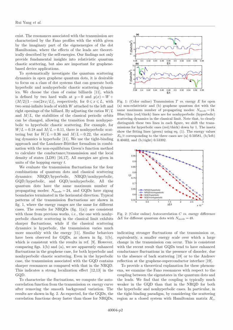
combinations of quantum dots and classical scatteringdynamics: NRQD/hyperbolic, NRQD/nonhyperbolic,GQD/hyperbolic, and GQD/nonhyperbolic. All thequantum dots have the same maximum number ofpropagating modes: Nmode = 24, and GQDs have zigzagboundaries terminated in the horizontal direction. Typicalpatterns of the transmission fluctuations are shown infig. 1, where the energy ranges are the same for differentcases. The results for NRQDs (fig. 1(a)) are consistentwith those from previous works, i.e., the one with nonhy-perbolic chaotic scattering in the classical limit exhibitssharper fluctuations, while if the classical scatteringdynamics is hyperbolic, the transmission varies muchmore smoothly with the energy [11]. Similar behaviorshave been observed for GQDs, as shown in fig. 1(b),which is consistent with the results in ref. [9]. However,comparing figs. 1(b) and (a), we see apparently enhancedfluctuations in the graphene case, for both hyperbolic andnonhyperbolic chaotic scattering. Even in the hyperboliccase, the transmission associated with the GQD containssharper resonances as compared with that in the NRQD.This indicates a strong localization effect [12,13] in theGQD.To characterize the fluctuations, we compute the auto-

correlation function from the transmission vs. energy curveafter removing the smooth background variation. Theresults are shown in fig. 2. As expected, for the GQDs, thecorrelation functions decay faster than those for NRQDs,

0.38 0.4 0.42 0.44 0.46 0.48 0.5 0.52 0.54 0.56 0.58

2

4

6

8

E/t

T (

Gxh

/2e2 )

0.38 0.4 0.42 0.44 0.46 0.48 0.5 0.52 0.54 0.56 0.580

2

4

6

8

10

E/t

T (

Gxh

/2e2 )

(a)

(b)

Fig. 1: (Color online) Transmission T vs. energy E for open(a) non-relativistic and (b) graphene quantum dot with thesame maximum number of propagating modes: Nmode = 24.Blue/thin (red/thick) lines are for nonhyperbolic (hyperbolic)scattering dynamics in the classical limit. Note that, to clearlydistinguish these two lines in each figure, we shift the trans-missions for hyperbolic ones (red/thick) down by 1. The insetsshow the fitting lines (green) using eq. (1). The energy valuesE0/t corresponding to the three cases are (a) 0.50581, (b/left)0.40402, and (b/right) 0.53392.

0 0.5 1 1.5 2 2.5 3

x 10−3

0.55

0.6

0.65

0.7

0.75

0.8

0.85

0.9

0.95

1

∆E/t

C

NRQD/hyperbolicNRQD/nonhyperbolicGQD/hyperbolicGQD/nonhyperbolic

Fig. 2: (Color online) Autocorrelation C vs. energy difference∆E for different quantum dots with Nmode = 48.

indicating stronger fluctuations of the transmission or,equivalently, a smaller energy scale over which a largechange in the transmission can occur. This is consistentwith the recent result that GQDs tend to have enhancedconductance fluctuations in the presence of disorder, dueto the absence of back scattering [18] or to the Andreevreflection at the graphene-superconductor interface [19].To provide a theoretical explanation for these phenom-

ena, we examine the Fano resonances with respect to thecoupling between the eigenstates in the quantum dots andthe leads. We find that the coupling is typically muchweaker in the GQD than that in the NRQD for boththe hyperbolic and nonhyperbolic cases. In particular, inthe tight-binding paradigm, by considering the scatteringregion as a closed system with Hamiltonian matrix Hc,

40004-p2

Quantum chaotic scattering in graphene systems

the effect of the leads can be treated using the retardedself-energy matrices, ΣR =ΣRL +Σ

RR. The matrix Hc is

Hermitian with a set of real eigenenergies and eigenfunc-tions {E0α, ψ0α|α= 1, . . . , N}, but ΣR(E) is in generalnot Hermitian and depends on the Fermi energy E. Theeffective Hamiltonian matrix Hc+Σ

R(E) thus has a setof complex eigenenergies with the eigenfunctions: [Hc+ΣR(E)]ψα =Eαψα and φTα [Hc+Σ

R(E)] =E∗αφTα , whereEα =E0α−∆α− iγα. The self-energy matrix ΣR has onlynonzero elements in the subblock of the boundary atomsconnecting with the leads. For most of the eigenstates itcan be treated as a perturbation, thus ∆α and γα aregenerally small.The Green’s function matrix can be expanded as

GR(E) =∑β [ψβ(E)φβ(E)

†]/[E−Eβ(E)]. For a partic-ular eigenstate {Eα, ψα}, when E is close to Eα,GR can be rewritten as GR =GR0 (E)+G

R1 (E), where

GR0 (E) =∑β �=α[ψβ(E)φβ(E)

†]/[E−Eβ(E)] varies slowlysince |E−Eβ | is large and GR1 (E) = [ψα(E)φα(E)†]/[E−Eα(E)] changes fast as E is in the vicinity of Eα. Theself-energy ΣR is a slow variable, so is the coupling matrixΓRL,R = i[Σ

RL,R− (ΣRL,R)†]. Thus in the expression of the

transmission T =Tr[ΓRLGRΓRR(G

R)†], only GR1 (E) is a fastvariable. All the others can be treated approximately asconstants and be evaluated at an arbitrary energy E0 closeto Eα. Choosing E0 =Eα, we get the transmission in thevicinity of Eα as T (E)≈ T0(E0)+∆T (1− 2qε)/(ε2+1),where T0 =Tr[Γ

RLG

R0 ΓRR(G

R0 )†], ∆= T (E0)−T0(E0), q=

Im(Tr[ΓRLGR1 ΓRR(G

R0 )†])/∆T , and ε= (E−Re(Eα))/γα.

We thus have

T (E)≈ T0(E0)−∆T +∆T (ε− q)2

ε2+1+∆T

2− q2ε2+1

. (1)

As shown in fig. 1, this formula agrees with numericalresults very well, which represents a generalized Fanoresonance, and is consistent with previous works onFano resonance profiles of conductance by calculating thescattering matrix elements [13,20]1. Thus the transmissioncurve has a resonance at Re(Eα), where the width is on theorder of γα. Since Σ

R depends on the energy E, ∆α and γαare also functions of E. Thus the above picture is valid onlyfor eigenstates whose values of Re(Eα) are close to E [17].The above analysis requires γα to be much smaller

than the level spacing between the adjacent energy levels,i.e., for separated and localized states. For large γα, theresonances are broadened and it then becomes difficultto distinguish them from the background variations.This is the reason that, for NRQDs with nonhyperbolicscattering dynamics, a similar analysis can be validonly when strong localizations on stable periodic orbits

1In the Fano formula, (ε+ q)2/(ε2+1), the quantity q usuallytakes on real values. However, as pointed out in ref. [20], whencharacterizing conductance fluctuations, q can generally be complex:q= q′+ iq′′. In this case, the Fano profile becomes |ε+ q|2/(ε2+1) =[(ε+ q′)2+ q′′2]/(ε2+1), which is the same as eq. (1) when q′2+q′′2 = 2. A similar relation was observed in a previous experimentalstudy [21].

0 0.2 0.4 0.6 0.8 110

−6

10−4

10−2

100

γ α/t

Re(Eα)/t

0 0.2 0.4 0.6 0.8 110

−6

10−4

10−2

100

γ α/t

Re(Eα)/t

0 0.5 1 1.5 210

−6

10−4

10−2

100

γ α/t

Re(Eα)/t

0 0.5 1 1.5 210

−6

10−4

10−2

100

Re(Eα)/t

γ α/t

(b)

(c) (d)

(a)

Fig. 3: (Color online) The real and imaginary part of theeigenstates Eα for (a) GQD/nonhyperbolic, (b) NRQD/nonhyperbolic, (c) GQD/hyperbolic, and (d) NRQD/hyperbolic. The energy values E0 in (a)–(d) are 0.2, 1, 0.2 and1, respectively.

occur [13]. For GQDs, our computations have revealedsharp conductance resonances (figs. 1 and 2) for bothhyperbolic and nonhyperbolic classical scattering dynam-ics, leading to small values of γα. Figure 3 shows theeigenenergies Eα in the complex plane in a proper energyrange. The energy for which the self-energy matrix isevaluated is E0 = 0.2t for GQDs and E0 = t for NRQDs.In principle, the plots are only accurate for the eigenen-ergies where Re(Eα) is close to E0 but we find that, evenif Re(Eα) is far from E0, it is still a good approximation.We have also examined larger systems with the sameshapes. For a larger system, there are more points in theplots, but the distribution of the points remains the same.These results verify those in fig. 2 in that the systemwith smaller γα values decreases faster in the correlationfunction. From fig. 3, we see that, the four cases havethe common feature that they all possess a continuousline shape about γα ∼ 10−2t. These values contribute tothe conductance variations on energy scales of 10−2t to10−1t and hence to the smooth conductance variationsin the background. For NRQDs, only the hyperbolic casehas this part, but the nonhyperbolic case has relativelylower values in the range 10−4t to 10−2t (fig. 3(b)),which correspond to the localized states. The separationbetween the two parts is not sharp, due to the hetero-geneous, mixed phase-space structure associated withnonhyperbolic chaotic scattering [12]. For GQDs, for boththe hyperbolic and nonhyperbolic cases, the distributionsof the eigenenergies contain two parts: one with and theother without localized states. For the nonhyperboliccase, the two parts are well separated and the lower part isseveral orders of magnitude smaller than that associatedwith the nonhyperbolic NRQD, as shown in fig. 3(a),indicating much sharper transmission fluctuations.Furthermore, the hyperbolic GQD also contains such a

40004-p3

Rui Yang et al.

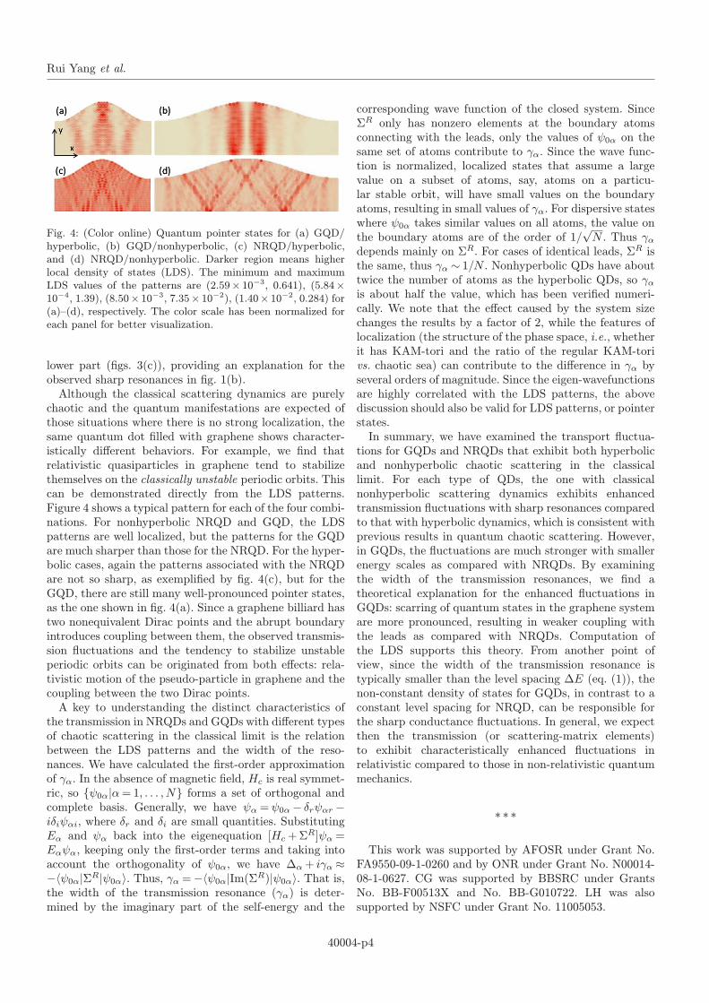
Fig. 4: (Color online) Quantum pointer states for (a) GQD/hyperbolic, (b) GQD/nonhyperbolic, (c) NRQD/hyperbolic,and (d) NRQD/nonhyperbolic. Darker region means higherlocal density of states (LDS). The minimum and maximumLDS values of the patterns are (2.59× 10−3, 0.641), (5.84×10−4, 1.39), (8.50× 10−3, 7.35× 10−2), (1.40× 10−2, 0.284) for(a)–(d), respectively. The color scale has been normalized foreach panel for better visualization.

lower part (figs. 3(c)), providing an explanation for theobserved sharp resonances in fig. 1(b).Although the classical scattering dynamics are purely

chaotic and the quantum manifestations are expected ofthose situations where there is no strong localization, thesame quantum dot filled with graphene shows character-istically different behaviors. For example, we find thatrelativistic quasiparticles in graphene tend to stabilizethemselves on the classically unstable periodic orbits. Thiscan be demonstrated directly from the LDS patterns.Figure 4 shows a typical pattern for each of the four combi-nations. For nonhyperbolic NRQD and GQD, the LDSpatterns are well localized, but the patterns for the GQDare much sharper than those for the NRQD. For the hyper-bolic cases, again the patterns associated with the NRQDare not so sharp, as exemplified by fig. 4(c), but for theGQD, there are still many well-pronounced pointer states,as the one shown in fig. 4(a). Since a graphene billiard hastwo nonequivalent Dirac points and the abrupt boundaryintroduces coupling between them, the observed transmis-sion fluctuations and the tendency to stabilize unstableperiodic orbits can be originated from both effects: rela-tivistic motion of the pseudo-particle in graphene and thecoupling between the two Dirac points.A key to understanding the distinct characteristics of

the transmission in NRQDs and GQDs with different typesof chaotic scattering in the classical limit is the relationbetween the LDS patterns and the width of the reso-nances. We have calculated the first-order approximationof γα. In the absence of magnetic field, Hc is real symmet-ric, so {ψ0α|α= 1, . . . , N} forms a set of orthogonal andcomplete basis. Generally, we have ψα =ψ0α− δrψαr −iδiψαi, where δr and δi are small quantities. SubstitutingEα and ψα back into the eigenequation [Hc+Σ

R]ψα =Eαψα, keeping only the first-order terms and taking intoaccount the orthogonality of ψ0α, we have ∆α+ iγα ≈−〈ψ0α|ΣR|ψ0α〉. Thus, γα =−〈ψ0α|Im(ΣR)|ψ0α〉. That is,the width of the transmission resonance (γα) is deter-mined by the imaginary part of the self-energy and the

corresponding wave function of the closed system. SinceΣR only has nonzero elements at the boundary atomsconnecting with the leads, only the values of ψ0α on thesame set of atoms contribute to γα. Since the wave func-tion is normalized, localized states that assume a largevalue on a subset of atoms, say, atoms on a particu-lar stable orbit, will have small values on the boundaryatoms, resulting in small values of γα. For dispersive stateswhere ψ0α takes similar values on all atoms, the value onthe boundary atoms are of the order of 1/

√N . Thus γα

depends mainly on ΣR. For cases of identical leads, ΣR isthe same, thus γα ∼ 1/N . Nonhyperbolic QDs have abouttwice the number of atoms as the hyperbolic QDs, so γαis about half the value, which has been verified numeri-cally. We note that the effect caused by the system sizechanges the results by a factor of 2, while the features oflocalization (the structure of the phase space, i.e., whetherit has KAM-tori and the ratio of the regular KAM-torivs. chaotic sea) can contribute to the difference in γα byseveral orders of magnitude. Since the eigen-wavefunctionsare highly correlated with the LDS patterns, the abovediscussion should also be valid for LDS patterns, or pointerstates.In summary, we have examined the transport fluctua-

tions for GQDs and NRQDs that exhibit both hyperbolicand nonhyperbolic chaotic scattering in the classicallimit. For each type of QDs, the one with classicalnonhyperbolic scattering dynamics exhibits enhancedtransmission fluctuations with sharp resonances comparedto that with hyperbolic dynamics, which is consistent withprevious results in quantum chaotic scattering. However,in GQDs, the fluctuations are much stronger with smallerenergy scales as compared with NRQDs. By examiningthe width of the transmission resonances, we find atheoretical explanation for the enhanced fluctuations inGQDs: scarring of quantum states in the graphene systemare more pronounced, resulting in weaker coupling withthe leads as compared with NRQDs. Computation ofthe LDS supports this theory. From another point ofview, since the width of the transmission resonance istypically smaller than the level spacing ∆E (eq. (1)), thenon-constant density of states for GQDs, in contrast to aconstant level spacing for NRQD, can be responsible forthe sharp conductance fluctuations. In general, we expectthen the transmission (or scattering-matrix elements)to exhibit characteristically enhanced fluctuations inrelativistic compared to those in non-relativistic quantummechanics.

∗ ∗ ∗

This work was supported by AFOSR under Grant No.FA9550-09-1-0260 and by ONR under Grant No. N00014-08-1-0627. CG was supported by BBSRC under GrantsNo. BB-F00513X and No. BB-G010722. LH was alsosupported by NSFC under Grant No. 11005053.

40004-p4

Quantum chaotic scattering in graphene systems

REFERENCES

[1] See, for example, Gutzwiller M. C., Chaos in Clas-sical and Quantum Mechanics (Springer, New York)1990; Stockmann H. J., Quantum Chaos: An Introduc-tion (Cambridge University Press, Cambridge, UK) 1999;Heller E. J., Phys. Rev. Lett., 53 (1984) 1515.

[2] Wallace P. R., Phys. Rev., 71 (1947) 622.[3] Castro Neto A. H., Guinea F., Peres N. M. R.,Novoselov K. S. and Geim A. K., Rev. Mod. Phys.,81 (2009) 109.

[4] Novoselov K. S., Geim A. K., Morozov S. V.,Jiang D., Zhang Y., Dubonos S. V., Grigorieva

I. V. and Firsov A. A., Science, 306 (2004) 666;Novoselov K. S., Geim A. K., Morozov S. V., Jiang

D., Katsnelson M. I., Grigorieva I. V., Dubonos

S. V. and Firsov A. A., Nature, 438 (2005) 197.[5] Amanatidis I. and Evangelou S. N., Phys. Rev.B, 79 (2009) 205420; Libisch F., Stampfer C. andBurgdofer J., Phys. Rev. B, 79 (2009) 115423; WurmJ. et al., Phys. Rev. Lett., 102 (2009) 056806; Huang L.,Lai Y.-C., Ferry D. K., Goodnick S. M. and AkisR., Phys. Rev. Lett., 103 (2009) 054101; Huang L., LaiY.-C. and Grebogi C., Phys. Rev. E, 81 (2010)055203(R); Chaos, 21 (2011) 013102.

[6] Blumel R. and Smilansky U., Phys. Rev. Lett., 60(1988) 477; Physica D, 36 (1989) 111.

[7] Doron E., Smilansky U. and Frenkel A., Phys. Rev.Lett., 65 (1990) 3072.

[8] Lai Y.-C., Blumel R., Ott E. and Grebogi C., Phys.Rev. Lett., 68 (1992) 3491.

[9] Bardarson J. H., Titov M. and Brouwer P. W.,Phys. Rev. Lett., 102 (2009) 226803.

[10] For quantum-dot systems whose classical dynamics arenonhyperbolic, it was demonstrated using semiclassicaltheory (Ketzmerick R., Phys. Rev. B, 54 (1996) 10841)and in experiments (Taylor R. P. et al., Phys. Rev.Lett., 78 (1997) 1952; Sachrajda A. S. et al., Phys.Rev. Lett., 80 (1998) 1948; Casati G., Guarneri I. andMaspero G., Phys. Rev. Lett., 84 (2000) 63; CrookR. et al., Phys. Rev. Lett., 91 (2003) 246803) that theconductance exhibits fractal fluctuation patterns due to

the hierarchical phase-space structure. An examinationof the Wigner time delay and the resonance width of theconductance profile reveals that, although a power-lawdistribution exists for the resonance width, as in agree-ment with the semiclassical prediction, the energy scale isin contrast far below the mean energy level spacing [11].It was then shown that the narrow resonances are in factcaused by the weak coupling between the localized statesaround the stable periodic orbits and the leads, whichonly couple to the chaotic part of the phase space [12,13],and the resonance line shape is well described by theFano profile (Fano U., Phys. Rev., 124 (1961) 1866).The tunneling between the chaotic part and the stableKAM island has been investigated numerically (BackerA., Ketzmerick R. and Monastra A. G., Phys. Rev.Lett. 94 (2005) 054102; Lock S., Backer A., Ketzmer-ick R. and Schlagheck P., Phys. Rev. Lett., 104 (2010)114101) and experimentally (de Moura A. P. S., LaiY.-C., Akis R., Bird J. and Ferry D. K., Phys. Rev.Lett., 88 (2002) 236804; Backer A. et al., Phys. Rev.Lett., 100 (2008) 174103).

[11] Huckestein B., Ketzmerick R. and LewenkopfC. H., Phys. Rev. Lett., 84 (2000) 5504.

[12] Weingartner B., Rotter S. and Burgdorfer J.,Phys. Rev. B, 72 (2005) 115342.

[13] Mendoza M., Schulz P. A., Vallejos R. O. andLewenkopf C. H., Phys. Rev. B, 77 (2008) 155307.

[14] Zurek W. H., Rev. Mod. Phys., 75 (2003) 715.[15] Huang L., Lai Y.-C., Ferry D. K., Goodnick S. M.

and Akis R., Phys. Rev. Lett., 103 (2009) 054101.[16] Landauer R., Philos. Mag., 21 (1970) 863.[17] Datta S., Electronic Transport in Mesoscopic Systems

(Cambridge University Press, Cambridge, UK) 1995.[18] Rycerz A., Tworzydlo J. and Beenakker C. W. J.,

EPL, 79 (2007) 57003.[19] Trbovic J., Minder N., Freitag F. and

Schonenberger C., Nanotechnology, 21 (2010) 274005.[20] Nakanishi T., Terakura K. and Ando T., Phys. Rev.

B, 69 (2004) 115307.[21] Kobayashi K., Aikawa H., Katsumoto S. and Iye Y.,

Phys. Rev. Lett., 88 (2002) 256806; Phys. Rev. B, 68(2003) 235304.

40004-p5