1

Quantification of fossil fuel CO2 emissions at the building/street scale for a large US city

Kevin R. Gurney, Igor Razlivanov, Yang Song School of Life Sciences, Arizona State University, Tempe, AZ, 85287

kevin.gurney@asu.edu

Yuyu Zhou

Joint Global Change Research Institute, Pacific Northwest National Laboratory, College Park, MD, 20770

Bedrich Benes, Michel Abdul-Massih

Department of Computer Graphics Technology, Purdue University, West Lafayette, IN, 47907 ABSTRACT In order to advance the scientific understanding of carbon exchange with the land surface, build an effective carbon monitoring system and contribute to quantitatively-based U.S. climate change policy interests, fine spatial and temporal quantification of fossil fuel CO2 emissions, the primary greenhouse gas, is essential. Called the ‘Hestia Project’, this research effort is the first to use bottom-up methods to quantify all fossil fuel CO2 emissions down to the scale of individual buildings, road segments, and industrial/electricity production facilities on an hourly basis for an entire urban landscape. a large city (Indianapolis, Indiana USA). Here, we describe the methods used to quantify the on-site fossil fuel CO2 emissions across the city of Indianapolis, Indiana. This effort combines a series of datasets and simulation tools such as a building energy simulation model, traffic data, power production reporting and local air pollution reporting. The system is general enough to be applied to any large U.S. city and holds tremendous potential as a key component of a carbon monitoring system in addition to enabling efficient greenhouse gas mitigation and planning. We compare our estimate of fossil fuel emissions from natural gas to consumption data provided by the local gas utility. At the zip code level, we achieve a bias-adjusted pearson r correlation value of 0.92 (p<0.001). INTRODUCTION Carbon dioxide (CO2) emission from fossil fuel combustion is the largest net annual flux of carbon to the atmosphere and represents the dominant source of greenhouse gas forcing 1,2. Fossil fuel CO2 emissions are often used as a near-certain boundary condition when solving total carbon budgets; an endeavor essential to quantifying other components of the carbon cycle and to improving our understanding of the feedbacks between the carbon cycle and climate change 3. Similarly, in order to construct meaningful projections of greenhouse gas emissions, a mechanistically-based quantification of current emissions is necessary. Finally, greenhouse gas mitigation efforts require improved quantification of fluxes in order to establish emission baselines, verify emission trajectories, and for the identification of efficient, economically-viable mitigation options 4. An important attribute of fossil fuel CO2 quantification is the space and time scale considered. A number of international and national agencies collect and report on emissions at the national and global scales and most commonly at annual timesteps 5. Spatial proxies have been commonly used to quantify spatial distribution of globally comprehensive emissions at the sub-national scales 6-9. Regional efforts at sub-national quantification have also been accomplished, often relying on a mixture of space and time proxies in addition to bottom-up data such as pollution emissions and fuel consumption statistics 10-13.

2

However, recently emerging scientific and decision support needs, require another step in emissions resolution down to the scale of the urban landscape. The density of atmospheric measurements of CO2 and its isotopic signature are increasing and the measurement network is becoming multi-tiered, including satellite, aircraft, flux tower, and surface air sampling 14-16. The increasing density is offering the opportunity to better understand the mechanisms driving land-atmosphere carbon exchange which occur at the scale of a forest plot or urban road segment. The ability to measure atmospheric CO2 and its isotopic signature at scales that might isolate fossil fuel emissions from the biological exchange in addition to discernment of discrete entities such as power plants and roadways, requires us to also build emissions estimates from the “bottom up” through higher resolution source quantification 17,18. Furthermore, construction of higher resolution, mechanistically-based fossil fuel CO2 emission estimation assists in better quantification and understanding of other pollutants such as CO and black carbon 19. These atmospheric/inventory measurement and model needs are driven, in part, by monitoring, reporting and verification (MRV) requirements that are emerging or anticipated to emerge at local, national, and international levels 20-23. Similarly important are information needs to plan and optimize fossil fuel CO2 mitigation strategies. For example, should emissions mitigation policy such as a cap-and-trade system become law, initial allocations and mitigation targets will be established 24. In order to meet such mitigation targets, action will be taken at local levels where industry functions, consumers live and power is produced. It is at these scales that quantitative information on emissions baselines and mitigation options are most readily needed and it is at the urban landscape scale that knowledge about local mitigation options, costs, and opportunities are the greatest 25-29. Focus on the urban domain is driven in no small part by the recognition that 51% of the world’s population resided in cities in 2010 and that share is projected to grow to 68% by 2050 30. Moreover, the rise of the megacity (over 10 million inhabitants) emphasizes the magnitude and trend towards global urbanization 31. Hence, efforts to better understand the carbon cycle and its interaction with climate at the urban landscape scale offer an intellectual connection to the growing research on urban sustainability and urban metabolic systems 32-34. Current research aimed at quantifying fossil fuel CO2 at the urban landscape scale typically stops at the level of the whole city or the census tract. For example, a number of studies have quantified fossil fuel CO2 emissions at the scale of an entire county or city 4,35-40. Other studies have attempted somewhat smaller spatial scales by quantifying emissions at the census tract or “community” level 41. As yet, no peer-reviewed research has attempted comprehensive quantification of fossil fuel CO2 emissions at the scales of individual buildings or neighborhoods for the entirety of an urban landscape. In this study, called the “Hestia” project, we quantify all on-site fossil fuel CO2 emissions at the building/road level every hour for the entire city of Indianapolis, USA. This study aims to establish an approach to quantify high resolution on-site fossil fuel CO2 emissions across an entire urban landscape that can be reproduced across the US while maintaining quantitative linkages to a national-level greenhouse gas accounting system 42. The method and results we describe here reflect the on-site fossil fuel combustion within the physical domain of the city excluding upstream or life-cycle associated emissions. Hence, emissions associated with material consumed within, but produced outside, the city is not reflected in the emissions estimation nor is electricity consumption within the city but which is generated outside of the city. In the Methods section we describe the study area and the methods by which we quantify each emitting economic sector to the building/road spatial scale and hourly time scale. In the Results and Discussion section we provide results and discuss the drivers and the space and time patterns resulting from the estimation approach. We conclude with comparison to independent data from the local natural gas utility.

3

BODY Methods Indianapolis, Indiana is the study area for the estimation approach described in this paper. Indianapolis is the county seat of Marion County which has boundaries nearly identical to those of the city of Indianapolis. Since most of original data sources are reported at the county level, we performed analysis for the Marion County domain, though the results are valid for either the County or City given their close spatial correspondence. The city contains nine Townships: Pike, Washington, Lawrence, Wayne, Center, Warren, Decatur, Perry, and Franklin. The city is located on a flat plain and is relatively symmetrical, with growth extending in all directions. It is an “island” city in the sense that it is surrounded in all directions by rural land-use, primarily cropland. This makes both atmospheric monitoring and CO2 inflow boundary questions more tractable as large upwind fossil fuel sources are well-mixed by the time they reach the Indianapolis area. As the capital of the state of Indiana, Indianapolis was listed as the 12th largest city in the U.S. in 2010 with a population of 820,445 43. The methodology used to quantify fossil fuel CO2 emissions start with the estimates generated by the Vulcan Project in Marion County 10,44. These emissions and the additional methods employed to downscale into the urban domain can be categorized by the original Vulcan data sources which roughly follow economic sectors. Table 1 provides the breakdown of the Vulcan fossil fuel CO2 emissions for Marion County disaggregated by data source, sector and fuel category. Two sectors, in particular, require considerable downscaling effort when starting with the Vulcan estimate. Buildings in which commercial, residential or industrial activities occur are estimated at the individual building level, starting from the census tract scale as estimated by Vulcan. Onroad transportation is downscaled from the county-level Vulcan emissions estimate, characterized by vehicle and road types. The downscaling utilizes local traffic count data. Non-point residential and commercial buildings Fossil fuel CO2 emissions associated with residential and commercial buildings in the city of Indianapolis reflect on-site combustion of fossil fuels only. Consumption of electricity and the associated emissions are located at the electricity generation location. The methodology employed for building emissions has been described in detail elsewhere 45. However, some improvements and corrections have been made to the original approach and those are described in Supplementary Information text along with a summary of the overall non-point residential and commercial building emissions methodology. Industrial non-point buildings Lacking classification in the model used to quantify energy use within buildings, and limited information from the DOE/EIA on industrial EUI values, the non-point industrial buildings in Marion County were estimated using a different approach than used for the residential and commercial sectors. Here, we construct carbon intensity values (mass of carbon emitted per unit floor area) from national statistics and combine this with the building parcel (BP) data layer to arrive at a building-by-building carbon emissions estimate [SI test 1]. Carbon intensity (CI) for industrial buildings was calculated by dividing national total annual CO2 emissions by the national total building floor area within each industrial sector 46,47. Industrial sectors are classified by the The North American Industry Classification System NAICS categories 48. As with the residential and commercial buildings, we can separate industrial buildings with and without natural gas service. Those with natural gas service were allocated the CO2 emissions associated with the county-level non-point industrial natural gas consumption. 1,894 (63%) industrial buildings had no

4

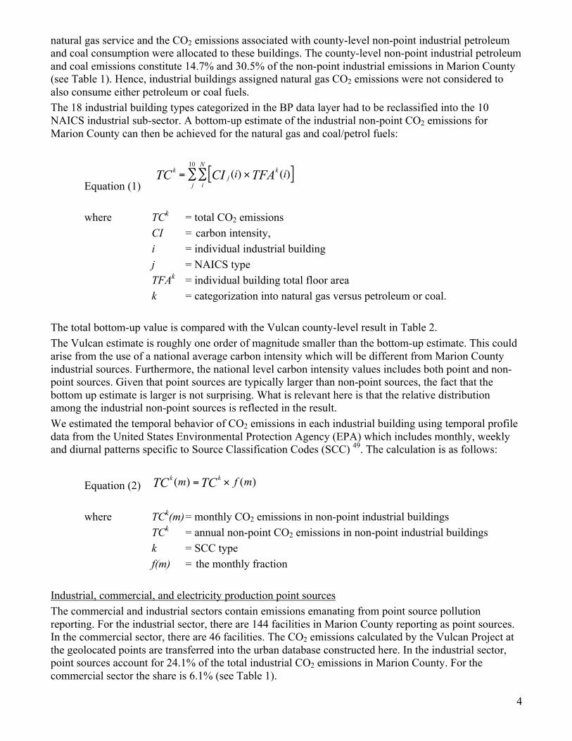
natural gas service and the CO2 emissions associated with county-level non-point industrial petroleum and coal consumption were allocated to these buildings. The county-level non-point industrial petroleum and coal emissions constitute 14.7% and 30.5% of the non-point industrial emissions in Marion County (see Table 1). Hence, industrial buildings assigned natural gas CO2 emissions were not considered to also consume either petroleum or coal fuels. The 18 industrial building types categorized in the BP data layer had to be reclassified into the 10 NAICS industrial sub-sector. A bottom-up estimate of the industrial non-point CO2 emissions for Marion County can then be achieved for the natural gas and coal/petrol fuels:

Equation (1)

€

kTC = jCI (i) × kTFA (i)[ ]i

N

∑j

10

∑

where TCk = total CO2 emissions

CI = carbon intensity, i = individual industrial building j = NAICS type TFAk = individual building total floor area k = categorization into natural gas versus petroleum or coal.

The total bottom-up value is compared with the Vulcan county-level result in Table 2. The Vulcan estimate is roughly one order of magnitude smaller than the bottom-up estimate. This could arise from the use of a national average carbon intensity which will be different from Marion County industrial sources. Furthermore, the national level carbon intensity values includes both point and non-point sources. Given that point sources are typically larger than non-point sources, the fact that the bottom up estimate is larger is not surprising. What is relevant here is that the relative distribution among the industrial non-point sources is reflected in the result. We estimated the temporal behavior of CO2 emissions in each industrial building using temporal profile data from the United States Environmental Protection Agency (EPA) which includes monthly, weekly and diurnal patterns specific to Source Classification Codes (SCC) 49. The calculation is as follows:

Equation (2)

€

kTC (m) = kTC × f (m)

where TCk(m) = monthly CO2 emissions in non-point industrial buildings

TCk = annual non-point CO2 emissions in non-point industrial buildings k = SCC type f(m) = the monthly fraction

Industrial, commercial, and electricity production point sources The commercial and industrial sectors contain emissions emanating from point source pollution reporting. For the industrial sector, there are 144 facilities in Marion County reporting as point sources. In the commercial sector, there are 46 facilities. The CO2 emissions calculated by the Vulcan Project at the geolocated points are transferred into the urban database constructed here. In the industrial sector, point sources account for 24.1% of the total industrial CO2 emissions in Marion County. For the commercial sector the share is 6.1% (see Table 1).

5

The emissions from electricity production are primarily supplied by data obtained from the EPA Clean Air Market Division (CAMD) Emission Tracking System/Continuous Emissions Monitoring system (ETS/CEMs) data for Electrical Generating Units (EGUs) 50,51. Within Marion County, three facilities reporting through the CAMD and an additional seven facilities report through the National Emissions Inventory (NEI) source reporting due the small size of the facility generation. Transportation The Transportation sector contains estimates for onroad, nonroad and air travel transportation. The nonroad and air travel sub-sectors are derived from the Vulcan estimate and no additional downscaling in space or time is performed. Onroad emissions are further downscaled into the urban landscape starting with the Marion County Vulcan estimate specific to month, vehicle type and road type. The Vulcan emissions are based on a combination of county-level data from the National Mobile Inventory Model (NMIM) County Database (NCD) and standard internal combustion engine stoichiometry from the MOBILE6.2 combustion emissions model 10. The Vulcan estimate provides onroad CO2 emissions for six road types (3 urban and 3 rural) and 28 different vehicle classes. In order to distribute these county-level emissions in space, the geographic location of roads and the density of traffic flow were used and result in quantification of onroad emissions by vehicle type, road type, and road segment every hour of the day. Results and Discussion Space and time patterns: residential, commercial, industrial The spatial distribution of the residential, commercial and industrial buildings is presented in Figure 1. In general, the city exhibits a development and land-use pattern reflective of circular outward growth from the older city center to the newer suburban and commercial hubs on the outer transportation artery. The residential sector shows residential clustering in the center portion of the city in addition to satellite clusters on the outer ring interstate that connects newer suburban areas to the city center. The commercial buildings cluster around major arterial intersection nodes on the outer ring interstate in addition to substantial commercial development in the city center. The industrial sector buildings are more randomly clustered though there is correspondence to the major “spoke” interstates emanating from the center of the city, particularly the interstate that runs in a SW – NE trajectory (I-70) which is a major coast-to-coast interstate. Figure 2 shows the seasonal weekly and diurnal temporal structure of the residential, commercial and industrial building emissions aggregated for the whole city. For the diurnal cycle, residential emissions are elevated from roughly 5 pm to 7 am relative to the daytime hours. Peak emissions occur at 7 am and 6 pm when residential activity is considered to be at a maximum (preparing for work/school, dinner/family activities). Commercial/industrial emissions, by contrast, have maximum values during the daylight working hours with peaks at roughly 9 am and 6 pm. The latter is due to the overlap of daytime work shifts and the evening or nighttime work shifts particularly common in the retail commercial sector (Figure 2b). The seasonality of the diurnal patterns show a straightforward scaling of the time profile with Winter values larger than Summer values due to greater space heating needs when outdoor temperatures are lower. The weekly time structures also exhibit both sectoral and seasonal differences. The industrial and commercial sectors exhibit weekend declines relative to weekday values and overall larger emissions during Winter than Summer. The residential sector, by contrast, shows slight increases on weekend days compared to weekend days. Both the seasonal diurnal and weekly time profiles are a combination of the survey-based building “schedules” and the local external surface temperature statistics for Indianapolis in 2002.

6

Space and time patterns: onroad transportation The onroad CO2 emission quantified for each road segment is presented in Figure 3. Due to the fact that Marion County is the center of Metropolitan Area, most of the road types belong to the urban group. The source data contains no emissions for rural interstates and rural arterials though there are non-zero road lengths in those categories. Urban interstate and arterial roads comprise 15% of the total road length but 62% of total CO2 emission due to the much greater traffic volume on these road types. Figure 4 demonstrates this as the large interstate that circles the city (I-465) and the two large interstates that bisect the city (I-65 and I-70) dominate emissions. Urban minor arterials and major collectors represent 9.4% of the total road length but nearly 22% of the total CO2 emissions. By contrast, urban minor collectors and local roads represent 63.4% of the total road length but only 16.3% of the total CO2 emission [SI Table 6]. Among all the vehicle types [SI Table 7], Light-Duty Gasoline Vehicles constitute the largest CO2 emissions (489.9 ktC/year) with Light-Duty Gasoline Trucks (both 0-3750 lbs and 3751-5750 lbs) as the next largest emitting vehicle type category (339.7 ktC/year). Overall, fossil fuel CO2 emissions due to gasoline-fueled vehicles are 8x larger than diesel-fueled emissions. The diurnal cycle of onroad CO2 emissions displays temporal structure defined by aggregate vehicle class and day of the week (Figure 4). During weekdays, the whole-city traffic for light-duty vehicles (passenger cars) shows maxima in the 6 to 9 am and 3 to 8 pm time periods. The evening rush hour is of longer duration with a more gradual onset and decline than the morning rush hour. Heavy-duty vehicles show little to no rush hour pattern but remain elevated from roughly 6 am to 5 pm after which they exhibit a gradual decline between 5 and 8 pm. This is consistent with heavy-duty vehicles being engaged in primarily commercial travel (local and interstate) and hence, active throughout daytime hours 52. Weekend traffic, by contrast, exhibits consistent emissions throughout daytime hours for both the light-duty and heavy-duty vehicle groups with a long increase from 6 am to roughly noon. The weekday nighttime emissions for light-duty vehicles is near-zero whereas heavy-duty vehicles maintain small but non-zero emissions during this time, consistent with the presence of interstate commercial trucking. Interestingly, weekend light-duty vehicle emissions reach a minimum at roughly 4 am, staying somewhat elevated relative to weekday emissions in the late evening/early morning hours, consistent with greater social non-commercial activity on weekend nights. Space and time patterns: total emissions Figure 5 presents the total fossil fuel CO2 emissions for the city of Indianapolis. The large arterial roadways and general building patterns are the dominant features. Also shown is a 3D view of the downtown area showing the dominance of Harding St Station, a 1,996 MW nameplate capacity powerplant. Figure 6 presents the distribution of fossil fuel CO2 emissions by economic sector, township and month . Marion County includes 9 townships of near equal geographic are but varying population and commercial/industrial activity. Decatur township, with the largest overall fossil fuel CO2 emissions, contains the Harding St Station power generation facility. Decatur township is also home to the Indianapolis International Airport. These account for the large electricity production and airport emissions, respectively. The remaining seven townships have onroad emissions as their largest emitting sector with industrial activity notable in Wayne and Center townships. The seasonal profile of the fossil fuel emissions follows a similar Winter/Summer patters with Decatur township reflecting the electricity production variations of the Harding St. Power Station. Comparison to natural gas consumption data Independent data on natural gas consumption was acquired from Citizen’s Gas (CG), the local natural gas utility in Indianapolis serving Marion county. The data supplied by CG was disaggregated to zip

7

code for the year 2009 and as monthly county totals for the years 2000 to 2009. In order to compare the results presented here to the CG data, the fractional values in each zip code for the year 2009 were transferred to the year 2002 total. Hence, actual changes in spatial distribution at scales larger than zip code will generate differences in comparison to the Hestia estimate. Figure 7 provides a comparison of the estimates generated in this study with the CG data. The county-total Hestia estimate is roughly 17% larger than the CG estimate. Two explanations are possible. First, the Hestia estimate at the county level is derived directly from the Vulcan system. The non-point emissions are based on state-level sales of natural gas allocated to the counties in Indiana based on proxies such as number of households (residential sector), commercial employees (commercial sector), and manufacturing employees (industrial sector). The point source contribution is based on the calculation of emissions from CO emissions. Both contributions contain uncertainties: the allocation by proxies could misrepresent the county apportionment across the state; the CO calculation could be using emission factors that are not representative of the specific combustion process conditions. Second, there is anecdotal evidence that CG is not the only natural gas supplier in the county. More specifically, large industrial consumers may have individual contracts with natural gas suppliers. Figure 7a displays the comparison at the annual zip code level after removing the mean county-total difference between the Hestia and CG estimate. The explained variance is high (r2 = 0.84) though five zip codes contain emissions that are greater than, or equal to, 2 standard deviations from the 1:1 line. The county-total monthly distribution similarly shows reasonable correspondence with the total bias showing up primarily during January and February (Figure 7b). The research presented here is now part of a larger experiment in which atmospheric concentrations of CO2, CH4, CO, and Δ14CO2 are being measured from aircraft and ground-based instruments in and around Indianapolis. This experiment, called INFLUX, will constrain and define uncertainty in estimating carbon fluxes through improved measurement techniques, inverse modeling, and comparison to emissions data products. Comparison of a “top-down” approach to the “bottom-up” emissions estimation performed here, will offer an important contraint to the Hestia system results. This will form the first step towards a carbon monitoring system that will ultimately combine satellite, airborne and ground-based measurements with independent emissions estimation and nested atmospheric modeling to verify reported emission reductions. Future work on the Hestia Project will emphasize a number of research avenues. With the exception of transportation and electricity production, quantifying the time structure of emissions remains challenging. Though the time structure in the resdiential, commercial and industrial buildings is based on survey information, there remains considerable uncertainty when applying that information to the spatial domain of Indianapolis. Expansion to include quantification of CH4 emissions is planned and is part of the INFLUX experiment. Estimation will likely rely on assumptions about leak rates from large gas pipeline junctions and landfills. In the case of pipeline leaks, both the location and the temporal structure pose challenges as details about the characteristics of natural gas pipelines is not readily available. Calibration to independent observed data also remains challenging, particularly given the limited availability of utility consumption data. Voluntary collection of a stratified sample of energy consumption data could be one way to overcome this limitation. However, coordination, data reliability and incentives to participate all pose difficulties. Another avenue of future research is to link the Hestia system, focused on carbon emissions, to efforts aimed at quantifying the complete urban metabolism or uban life cycle. Urban metabolism research is typically focused on the consumption of energy and materials, their transformation and ultimate disposition in waste streams or goods. Linking these two approaches would require carbon emissions to be traced both upstream and downstream to the consumption activity driving the fossil fuel combustion. For example, carbon emissions associated with electricity generation are driven by electricity consumption at the end-use, both within Indianapolis and outside. Similarly, carbon emissios associated

8

with the manufacture of physical goods are driven by consumptive demand inside and outside Indianapolis. Conversely, emissions that occur elsewhere but are driven by consumptive activity within Indianapolis would require tracking. A similar effort to the research reported here has begun in the city of Los Angeles, California. Los Angeles is both larger in terms of population and spatial extent. Like the experiment in Indianapolis, comparison to a variety of atmospheric measurements offer further insight into how we can integrate bottom up fossil fuel CO2 emissions estimation with top-down measurement systems.

CONCLUSIONS

The Hestia Project is the first to use bottom-up methods solely to quantify all fossil fuel CO2 emissions down to the scale of individual buildings, road segments, and industrial/electricity production facilities on an hourly basis for an entire urban landscape. We have completeda large city (Indianapolis, Indiana USA). Here, we describe the methods used to quantify the on-site fossil fuel CO2 emissions across the city of Indianapolis, Indiana. This effort combines a series of datasets and simulation tools such as a building energy simulation model, traffic data, power production reporting and local air pollution reporting. The system is general enough to be applied to any large U.S. city and holds tremendous potential as a key component of a carbon monitoring system in addition to enabling efficient greenhouse gas mitigation and planning. We compare our estimate of fossil fuel emissions from natural gas to consumption data provided by the local gas utility. At the zip code level, we achieve a bias-adjusted pearson r correlation value of 0.92 (p<0.001). REFERENCES 1 Canadell, J. G. et al. Contributions to accelerating atmospheric CO2 growth from economic

activity, carbon intensity, and efficiency of natural sinks. Proceedings of the National Academy of Sciences of the United States of America 104, 18866-18870, doi:10.1073/pnas.0702737104 (2007).

2 Hansen, J. E. et al. Climate forcings in the Industrial era. Proceedings of the National Academy of Sciences of the United States of America 95, 12753-12758, doi:10.1073/pnas.95.22.12753 (1998).

3 Gurney, K. R. et al. Research needs for finely resolved fossil carbon emissions. Eos Trans. AGU 88, doi:10.1029/2007eo490008 (2007).

4 Kennedy, C. et al. Methodology for inventorying greenhouse gas emissions from global cities. Energy Policy 38, 4828-4837, doi:10.1016/j.enpol.2009.08.050 (2010).

5 Macknick, J. Energy and CO2 emission data uncertainties. Carbon Management 2, 189-205 (2011).

6 Rayner, P. J., Raupach, M. R., Paget, M., Peylin, P. & Koffi, E. A new global gridded data set of CO2 emissions from fossil fuel combustion: Methodology and evaluation. Journal of Geophysical Research-Atmospheres 115, doi:10.1029/2009jd013439 (2010).

7 Andres, R. J., Marland, G., Fung, I. & Matthews, E. A 1 degrees x1 degrees distribution of carbon dioxide emissions from fossil fuel consumption and cement manufacture, 1950-1990. Global Biogeochemical Cycles 10, 419-429, doi:10.1029/96gb01523 (1996).

8 Oda, T. & Maksyutov, S. A very high-resolution (1 km x 1 km) global fossil fuel CO2 emission inventory derived using a point source database and satellite observations of nighttime lights. Atmospheric Chemistry and Physics 11, 543-556, doi:10.5194/acp-11-543-2011 (2011).

9 Olivier, J. G. J. et al. Recent trends in global greenhouse gas emissions, regional trends 1970–2000 and spatial distribution of key sources in 2000. Environmental Sciences (15693430) 2, 81-99, doi:10.1080/15693430500400345 (2005).

9

10 Gurney, K. R. et al. High Resolution Fossil Fuel Combustion CO2 Emission Fluxes for the United States. Environmental Science & Technology 43, 5535-5541, doi:10.1021/es900806c (2009).

11 Gregg, J. S., Losey, L. M., Andres, R. J., Blasing, T. J. & Marland, G. The Temporal and Spatial Distribution of Carbon Dioxide Emissions from Fossil-Fuel Use in North America. Journal of Applied Meteorology and Climatology 48, 2528-2542, doi:10.1175/2009jamc2115.1 (2009).

12 Blasing, T. J., C.T. Broniak, and G. Marland State-by-state carbon dioxide emissions from fossil fuel use in the United States 1960-2000. Mitigation and Adaptation Strategies for Global Change 10, 659-674 (2005).

13 Ciais, P. et al. The European carbon balance. Part 1: fossil fuel emissions. Global Change Biology 16, 1395-1408, doi:10.1111/j.1365-2486.2009.02098.x (2010).

14 Turnbull, J. et al. On the use of 14CO2 as a tracer for fossil fuel CO2: Quantifying uncertainties using an atmospheric transport model. Journal of Geophysical Research-Atmospheres 114, doi:10.1029/2009jd012308 (2009).

15 Mays, K. L. et al. Aircraft-Based Measurements of the Carbon Footprint of Indianapolis. Environmental Science & Technology 43, 7816-7823, doi:10.1021/es901326b (2009).

16 Pataki, D. E., Bowling, D. R., Ehleringer, J. R. & Zobitz, J. M. High resolution atmospheric monitoring of urban carbon dioxide sources. Geophysical Research Letters 33, doi:10.1029/2005gl024822 (2006).

17 Riley, W. J. et al. Where do fossil fuel carbon dioxide emissions from California go? An analysis based on radiocarbon observations and an atmospheric transport model. Journal of Geophysical Research-Biogeosciences 113, doi:10.1029/2007jg000625 (2008).

18 Duren, R. M. & Miller, C. E. Towards robust global greenhouse gas monitoring. Greenhouse Gas Measurement and Management 1, 80-84, doi:10.1080/20430779.2011.579356 (2011).

19 Turnbull, J. C. et al. Atmospheric observations of carbon monoxide and fossil fuel CO2 emissions from East Asia. Journal of Geophysical Research-Atmospheres 116, doi:10.1029/2011jd016691 (2011).

20 Committee on Methods for Estimating Greenhouse Gas Emissions. Verifying Greenhouse Gas Emissions: Methods to Support International Climate Agreements. Report No. 9780309152112, (The National Academies Press, Washington DC, 2010).

21 Schakenbach, J., Vollaro, R. & Forte, R. Fundamentals of Successful Monitoring, Reporting, and Verification under a Cap-and-Trade Program. Journal of the Air & Waste Management Association 56, 1576-1583 (2006).

22 Vine, E. & Sathaye, J. The Monitoring, Evaluation, Reporting and Verification of Climate Change Projects. Mitigation and Adaptation Strategies for Global Change 4, 43-60, doi:10.1023/a:1009651316596 (1999).

23 Lutsey, N. & Sperling, D. America's bottom-up climate change mitigation policy. Energy Policy 36, 673-685, doi:10.1016/j.enpol.2007.10.018 (2008).

24 Hepburn, C. Carbon Trading: A Review of the Kyoto Mechanisms. Annual Review of Environment and Resources 32, 375-393, doi:doi:10.1146/annurev.energy.32.053006.141203 (2007).

25 Rosenzweig, C., Solecki, W., Hammer, S. A. & Mehrotra, S. Cities lead the way in climate-change action. Nature 467, 909-911 (2010).

26 Fleming, P. D. & Webber, P. H. Local and regional greenhouse gas management. Energy Policy 32, 761-771, doi:10.1016/s0301-4215(02)00339-7 (2004).

27 Salon, D. et al. City carbon budgets: A proposal to align incentives for climate-friendly communities. Energy Policy 38, 2032-2041, doi:10.1016/j.enpol.2009.12.005 (2010).

28 Betsill, M. M. & Bulkeley, H. Cities and the Multilevel Governance of Global Climate Change. Global Governance 12, 141-159 (2006).

29 Dhakal, S. & Shrestha, R. M. Bridging the research gaps for carbon emissions and their management in cities. Energy Policy 38, 4753-4755, doi:10.1016/j.enpol.2009.12.001 (2010).

10

30 United Nations. (United Nations Department of Economic and Social Affairs, Population Division, New York, 2010).

31 Gurjar, B. R. & Lelieveld, J. New Directions: Megacities and global change. Atmospheric Environment 39, 391-393, doi:10.1016/j.atmosenv.2004.11.002 (2005).

32 Kennedy, C., Cuddihy, J. & Engel-Yan, J. The Changing Metabolism of Cities. Journal of Industrial Ecology 11, 43-59, doi:10.1162/jie.2007.1107 (2007).

33 Decker, E. H., Elliott, S., Smith, F. A., Blake, D. R. & Rowland, F. S. Energy and Material Flow Through the Urban Ecosystem. Annual Review of Energy and the Environment 25, 685-740, doi:doi:10.1146/annurev.energy.25.1.685 (2000).

34 Grimm, N. B. et al. Global Change and the Ecology of Cities. Science 319, 756-760, doi:10.1126/science.1150195 (2008).

35 Parshall, L. et al. Modeling energy consumption and CO2 emissions at the urban scale: Methodological challenges and insights from the United States. Energy Policy 38, 4765-4782, doi:10.1016/j.enpol.2009.07.006 (2010).

36 Hillman, T. & Ramaswami, A. Greenhouse Gas Emission Footprints and Energy Use Benchmarks for Eight U.S. Cities. Environmental Science & Technology 44, 1902-1910, doi:10.1021/es9024194 (2010).

37 Sovacool, B. K. & Brown, M. A. Twelve metropolitan carbon footprints: A preliminary comparative global assessment. Energy Policy 38, 4856-4869, doi:10.1016/j.enpol.2009.10.001 (2010).

38 Ramaswami, A., Hillman, T., Janson, B., Reiner, M. & Thomas, G. A Demand-Centered, Hybrid Life-Cycle Methodology for City-Scale Greenhouse Gas Inventories. Environmental Science & Technology 42, 6455-6461, doi:10.1021/es702992q (2008).

39 Baldasano, J. M., Soriano, C. & Boada, L. s. Emission inventory for greenhouse gases in the City of Barcelona, 1987–1996. Atmospheric Environment 33, 3765-3775, doi:10.1016/s1352-2310(99)00086-2 (1999).

40 Ngo, N. & Pataki, D. The energy and mass balance of Los Angeles County. Urban Ecosystems 11, 121-139, doi:10.1007/s11252-008-0051-1 (2008).

41 VandeWeghe, J. R. & Kennedy, C. A Spatial Analysis of Residential Greenhouse Gas Emissions in the Toronto Census Metropolitan Area. Journal of Industrial Ecology 11, 133-144, doi:10.1162/jie.2007.1220 (2007).

42 Gurney, K. R. Policy Update: Observing human CO2 emissions. Carbon Management 2, 223-226, doi:10.4155/cmt.11.28 (2011).

43 United States Census Bureau. <http://2010.census.gov/2010census/popmap/ipmtext.php?fl=18> (2010).

44 Gurney, K. R. et al. Vulcan Science Methods Documentation, Version 2.0, <http://vulcan.project.asu.edu/pdf/Vulcan.documentation.v2.0.online.pdf> (2011).

45 Zhou, Y. & Gurney, K. A new methodology for quantifying on-site residential and commercial fossil fuel CO2 emissions at the building spatial scale and hourly time scale. Carbon Management 1, 45-56, doi:10.4155/cmt.10.7 (2010).

46 United States Energy Information Administration. 2006 Energy Consumption by Manufacturers--Data Tables, <http://www.eia.gov/emeu/mecs/mecs2006/2006tables.html> (2006).

47 Schipper, M. (ed Energy Information Administration (EIA)) (Washington DC, 2006). 48 United States Census Bureau. North American Industry Classification System,

<http://www.census.gov/eos/www/naics/> (2007). 49 United States Environmental Protection Agency. Emissions Modeling Clearinghouse Temporal

Allocation, <http://www.epa.gov/ttn/chief/emch/temporal/index.html> (2002). 50 Ackerman, K. V. & Sundquist, E. T. Comparison of Two U.S. Power-Plant Carbon Dioxide

Emissions Data Sets. Environmental Science & Technology 42, 5688-5693, doi:10.1021/es800221q (2008).

11

51 Petron, G., Tans, P., Frost, G., Chao, D. & Trainer, M. High-resolution emissions of CO2 from power generation in the USA. J. Geophys. Res. 113, G04008, doi:10.1029/2007jg000602 (2008).

52 Lindhjem, C. E. & Shepard, S. (ed USEPA) (ENVIRON Corporation, Novato, CA, 2007).

KEY WORDS High resolution greenhouse gas emissions Urban CO2 emissions Emission inventory

12

Table 1: Fossil fuel CO2 emissions for Marion County categorized by data source, sector and fuel. Units: MtC/yr Data

Source Non-point NEI† Point NEI

Point NEI/Point CAMD¶

NMIM NCD§ Transportation

Airport NEI

Sector Industrial Commercial Residential Industrial Commercial Electricity Production Onroad Nonroad Airport

Fuel Coal

Petrol

NG Coal

Petrol NG Coal Petrol NG Coal

Petrol NG Coal

Petrol NG Coal

Petrol NG Petrol Petrol Petrol

Emissions 0.10 0.05 0.19 0 0.06 0.27 0.004 0.009 0.35 0 0.017 0.092 0 0.003 0.018 1.0 0.008 0.030 1.07 0.13 0.17

† NEI refers to the United States Environmental Protection Agency National Emissions Inventory CO emissions reporting. See 10 for more information ¶ CAMD refers to the United States Environmental Protection Agency Clean Air Markets Division. § NMIM NCD refers to the National Mobile Inventory Model National County Database. Table 2: Indianapolis non-point industrial building fossil fuel CO2 emissions comparison

Sector Vulcan† (kgC/yr)

Bottom up (kgC/yr)

Vulcan-bottom up difference (%)

Vulcan/BU Ratio

IND (NG) 1.88E+08 8.62E+09 191.5 0.022

IND (Petrol/Coal) 1.55E+08 1.57E+09 164.0 0.099 † Marion County result from 10

13

Figure 1: Annual fossil fuel CO2 emissions for the a) residential, b) commercial and c) industrial sectors in Marion County, Indiana. Note the different scale in each panel. Units: Log10 kgC/yr.

14

Figure 2: Seasonal fossil fuel CO2 emissions for buildings in Indianapolis, Indiana. a) weekly temporal profiles for the residential, commercial and industrial sectors; b) diurnal temporal profiles for the residential, commercial and industrial sectors. Industrial (black), Commercial (blue), Residential (red), Summer (dashed), Winter (solid). The insets in b) show commercial (downtown) and residential sectors at 9 a.m and 6 p.m. Units: ktC/yr.

a) b)

15

Figure 3: Annual onroad CO2 emissions for Marion County, 2002. Major interstates are noted. Units: Log10 tC/yr

16

Figure 4: Onroad transportation annual mean diurnal fossil fuel CO2 emissions hourly fraction for light-duty (solid) and heavy-duty (dashed) vehicle class aggregates. a) weekday emissions; b) weekend emissions. Units: fraction of daily total.

a) b) Figure 5: Total fossil fuel CO2 emissions for Marion County, Indiana for the year 2002. a) top view with numbered zones. b) blowups of the numbered zones. Color units: Log10 kgC/yr; Box height units: Linear.

a) b)

17

Figure 6: 2002 Fossil fuel CO2 emissions for Marion County, Indiana. a) by sector for the 9 townships; b) monthly profile by township.

a) b)

Figure 7: Comparison of the summed residential, commercial and industrial building CO2 emissions from Citizen’s Gas versus this study due to natural gas consumption in Marion County. a) annual zip code comparison. Hestia values have been bias-adjusted. Also shown: 1:1 line (solid), 1 standard deviation (dashed), 2 standard deviation (dotted). Outlier zip codes noted. b) Monthly, county-total comparison; this study (solid), Citizen’s Gas (dashed). No bias adjustment.

a) b)