Linköping University Medical Dissertations No. 1374

Quantification of 4D Left Ventricular Blood Flow in Health and Disease

Jonatan Eriksson

Division of Cardiovascular Medicine Department of Medical and Health Sciences

Faculty of Health Sciences Center for Medical Image Science and Visualization

Linköping University, Sweden

Linköping, October, 2013

II

This work has been conducted within the Center for Medical Image Science and Visualization (CMIV) at Linköping University, Sweden. CMIV is acknowledged for provision of financial support and access to leading edge research infrastructure. Furthermore, the Swedish Heart-Lung foundation, the Swedish Research Council, the Emil and Vera Cornell Foundation, the Heart Foundation, the Center for Industrial Information Technology (CENIIT) and Eleanora Demeroutis Foundation are acknowledged for financial support. Quantification of 4D Left Ventricular Blood Flow in Health and Disease Linköping University Medical Dissertations No. 1374 Copyright © 2013 by Jonatan Eriksson unless otherwise stated No part of this work may be reproduced, stored in a retrieval system, or be transmitted, in any form or by any means, electronic, mechanic, photocopying, recording or otherwise, without prior written permission from the author. Division of Cardiovascular Medicine Department of Medical and Health Sciences Linköping University SE-581 85 Linköping Sweden http://www.liu.se/cmr ISBN 978-91-7519-542-1 ISSN 0345-0082 Printed by LiU-Tryck, Linköping, Sweden, 2013 Cover: Pathline visualization of systemic and pulmonary blood flow. Red through yellow is left heart flow (i.e. left atrium, left ventricle and aorta). While, blue is right heart flow (i.e. right atrium, right ventricle and pulmonary aorta). The morphological four-chamber image provides anatomical orientation.

III

“A good doctor looks at both, the pictures and the numbers. Science needs to work that way, too”

– Benoit Mandelbrot

IV

I

Abstract

The main function of the heart is to pump blood throughout the cardiovascular system by generating pressure differences created through volume changes. Although the main purpose of the heart and vessels is to lead the flowing blood throughout the body, clinical assessments of cardiac function are usually based on morphology, approximating the flow features by viewing the motion of the myocardium and vessels. Measurement of three-directional, three-dimensional and time-resolved velocity (4D Flow) data is feasible using magnetic resonance (MR). The focus of this thesis is the development and application of methods that facilitate the analysis of larger groups of data in order to increase our understanding of intracardiac flow patterns and take the 4D flow technique closer to the clinical setting. In the first studies underlying this thesis, a pathline based method for analysis of intra ventricular blood flow patterns has been implemented and applied. A pathline is integrated from the velocity data and shows the path an imaginary massless particle would take through the data volume. This method separates the end-diastolic volume (EDV) into four functional components, based on the position for each individual pathline at end-diastole (ED) and end-systole (ES). This approach enables tracking of the full EDV over one cardiac cycle and facilitates calculation of parameters such as e.g. volumes and kinetic energy (KE). Besides blood flow, pressure plays an important role in the cardiac dynamics. In order to study this parameter in the left ventricle, the relative pressure field was computed using the pressure Poisson equation. A comprehensive presentation of the pressure data was obtained dividing the LV blood pool into 17 pie-shaped segments based on a modification of the standard seventeen segment model. Further insight into intracardiac blood flow dynamics was obtained by studying the turbulent kinetic energy (TKE) in the LV. The methods were applied to data from a group of healthy subjects and patients with dilated cardiomyopathy (DCM). DCM is a pathological state where the cardiac function is impaired and the left ventricle or both ventricles are dilated. The validation study of the flow analysis method showed that a reliable user friendly tool for intra ventricular blood flow analysis was obtained. The application of this tool also showed that roughly one third of the blood that enters the LV, directly leaves the LV again in the same heart beat. The distribution of the four LV EDV components was altered in the DCM group as compared to the healthy group; the component that enters and leaves the LV during one cardiac cycle (Direct Flow) was significantly larger in the healthy subjects. Furthermore, when the kinetic energy was normalized by the volume for each component, at time of ED, the Direct Flow had the highest values in the healthy subjects. In the DCM group, however, the Retained Inflow and Delayed Ejection Flow had higher values. The relative pressure field showed to be highly heterogeneous, in the healthy heart. During diastole the predominate pressure differences in the LV occur along the long axis from base to apex. The distribution and variability of 3D pressure fields differ between early and late diastolic filling

II

phases, but common to both phases is a relatively lower pressure in the outflow segment. In the normal LV, TKE values are low. The highest TKE values can be seen during early diastole and are regionally distributed near the basal LV regions. In contrast, in a heterogeneous group of DCM patients, total diastolic and late diastolic TKE values are higher than in normals, and increase with the LV volume. In conclusion, in this thesis, methods for analysis of multidirectional intra cardiac velocity data have been obtained. These methods allow assessment of data quality, intra cardiac blood flow patterns, relative pressure fields, and TKE. Using these methods, new insights have been obtained in intra cardiac blood flow dynamics in health and disease. The work underlying this thesis facilitates assessment of data from a larger population of healthy subjects and patients, thus bringing the 4D Flow MRI technique closer to the clinical setting.

III

Populärvetenskaplig sammanfattning

Hjärt- och kärlsjukdomar hör till de vanligaste dödsorsakerna i Sverige och övriga västvärlden. Hjärtats huvudfunktion är att pumpa blod genom hjärt- och kärlsystemet. Blodflödet genom hjärt- och kärlsystemet drivs av tryckskillnader som skapas när hjärtmuskeln spänns och slappnar av. Blodet tar komplexa vägar genom hjärtats fyra rum där interaktion sker mellan olika flödesskikt och även mellan blodet och hjärtväggen. Blodet som pumpas ut i kroppen för med sig syre, näringsämnen och hormoner till cellerna och på sin väg tillbaka mot hjärta och lungor tar det med sig koldioxid och avfallsprodukter. Trots att hjärtats huvudsyfte är att driva blodflödet är majoriteten av den kliniska funktionsbedömningen baserad på väggrörelse. När flödesinformation används är den ofta mätt med hjälp av metoder där enbart en av de tre hastighetsriktningarna används. Med hjälp av magnetresonanskamera kan man mäta så kallat fyrdimensionellt flöde. Det vill säga att i en tredimensionell volym kan man tidsupplöst mäta blodets hastighet i tre riktningar. Den här avhandlingen fokuserar på utveckling och tillämpning av robusta och användarvänliga analysverktyg för denna typ av data, i syfte att kunna utnyttja den stora mängd information som finns och på sikt kunna ta denna typ av flödesinsamlingar närmare kliniken. I avhandlingens första tre studier implementeras, utvärderas och tillämpas en analysmetod för att studera blodets väg genom hjärtats vänstra kammare. Kortfattat går metoden ut på att rita ut konturerna av vänster kammare i anatomisk data och sedan beräkna så kallade partikelspår från hela kammarvolymen. Detta görs framåt (som att fråga varje del: vart ska du ta vägen?) och bakåt i det omvända flödet (som att fråga varje del: var kom du ifrån?) för att spåra hur blodet i vänster kammare färdats under en hjärtcykel. Ett partikelspår visar vägen som en masslös partikel skulle ta genom den tidsupplösta datavolymen. Den föreslagna metoden delar in den slutdiastoliska volymen i fyra funktionella komponenter baserat på varje partikelspårs position vid slutet av hjärtcykeln. I studie II, byggs denna metod ut med beräkningar av bl a kinetisk energi och tillämpas på en grupp friska personer. I studie III tillämpas verktygen på en grupp patienter med dilaterad kardiomyopati (DCM), detta är en sjukdom där hjärtats funktion försämras och hjärtats vänster och ibland även höger kammare förstoras och får mer rundad form. Fördelningen av de fyra funktionella komponenterna skiljde sig mellan friska och DCM-patienter. I studie IV används en tidigare presenterad metod för att beräkna relativa tryckfält i hjärtat och ett verktyg för att smidigare kunna utnyttja detta i flera dataset skapades. Vidare delas vänster kammare in i mindre segment för att göra analysresultaten mer översiktliga. I studie V summeras vänster kammarens turbulenskinetiska energi (TKE) som mätts med magnetresonans. Turbulens innebär att hastigheten i en punkt varierar kraftigt med snabba slumpmässiga svängningar. TKE är ett mått på hur intensiv denna variation är och kan ses som ett effektivitetsmått, eftersom TKE förloras som värme. En grupp med friska personer och en grupp med DCM inkluderades i denna studie. För att sammanfatta, studierna som utgör denna avhandling har visat att de utvecklade programmen tillåter studier av blodflödesmönster i större grupper av individer. Det i

IV

sin tur gör det möjligt att fastställa referensmaterial för friska personer och även på sikt för patienter. Även om det fortfarande finns begränsningar i alla steg har arbetena i denna avhandling tagit flerdimensionella flödesinsamlingar med MRI några steg närmare klinisk tillämpning.

V

List of papers

This thesis is based on the following five papers, which will be referred to by their roman numerals:

I. Semi-automatic quantification of 4D left ventricular blood flow. Jonatan Eriksson, Carl-Johan Carlhäll, Petter Dyverfeldt, Jan Engvall, Ann F. Bolger, Tino Ebbers. J Cardiovasc Magn Reson 2010;12(1):9.

II. Quantification of presystolic blood flow organization and energetics in the human left ventricle. Jonatan Eriksson, Petter Dyverfeldt, Jan Engvall, Ann F. Bolger, Tino Ebbers, Carl-Johan Carlhäll. Am J Physiol Heart Circ Physiol. 2011;300:H2135-H2141.

III. Four-dimensional blood flow-specific markers of LV dysfunction in dilated cardiomyopathy. Jonatan Eriksson, Ann F. Bolger, Tino Ebbers, and Carl-Johan Carlhäll. European Heart Journal – Cardiovascular Imaging. 2013;14:417–424

IV. Spatial heterogeneity of 4D relative pressure fields in the human left ventricle. Jonatan Eriksson, Ann F. Bolger, Carl-Johan Carlhäll, Tino Ebbers. In manuscript.

V. Turbulent kinetic energy in normal and myopathic left ventricles. Jacub Zajac, Jonatan Eriksson, Petter Dyverfeldt, Ann F. Bolger, Tino Ebbers, Carl-Johan Carlhäll. In manuscript.

VII

Abbreviations

3D = Three-dimensional 4D = Four-dimensional, here it is meant three-directional, time-resolved in a three-dimensional volume A-wave = Filling during the late phase of diastole, filling due to atrial contraction AoV = Aortic Valve BPM = Beats per minute CFD = Computational fluid dynamics Cine = Cinematography, refers to the collection of data over a complete cardiac cycle CO = Cardiac output CT = Computer tomography DCM = Dilated cardiomyopathy E-wave = Filling during the early phase of diastole, the relaxation dependent filling ED = End diastole EDV = End diastolic volume EF = Ejection fraction ES = End systole ESV = End systolic volume HR = Heart rate IVC = Isovolumetric contraction IVR = Isovolumetric relaxation IVSD = Intravoxel velocity standard deviation IVVV = Intravoxel velocity variation LVOT = Left ventricular outflow tract mmHg = Milli meters of mercury, a unit for pressure used clinically referring to the force per unit area to keep a column of one mm of mercury (Hg). 1 mmHg = 133 Pa MRI = Magnetic resonance imaging PC-MRI = Phase contrast magnetic resonance imaging Pixel = Picture element Std = Standard deviation SV = Stroke volume Voxel = Volume element, the three-dimensional equivalent of a pixel.

IX

Table of contents

ABSTRACT ............................................................................................................................................ I

POPULÄRVETENSKAPLIG SAMMANFATTNING.................................................................... III

LIST OF PAPERS................................................................................................................................. V

ABBREVIATIONS.............................................................................................................................VII

TABLE OF CONTENTS .................................................................................................................... IX

1 INTRODUCTION.........................................................................................................................1

2 AIMS..............................................................................................................................................3

3 BACKGROUND ...........................................................................................................................5

3.1 PHYSIOLOGICAL BACKGROUND..............................................................................................5 3.1.1 The heart...........................................................................................................................5 3.1.2 Cardiac function ...............................................................................................................6 3.1.3 Assessment of cardiac function.........................................................................................7 3.1.4 Dilated cardiomyopathy ...................................................................................................8

3.2 TECHNICAL BACKGROUND .....................................................................................................9 3.2.1 Magnetic resonance imaging and phase contrast MRI.....................................................9 3.2.2 Pressure..........................................................................................................................10 3.2.3 Turbulent kinetic energy .................................................................................................11

3.3 BLOOD FLOW VISUALIZATION ..............................................................................................12 3.3.1 Particle trace visualization.............................................................................................12 3.3.2 Isosurfaces ......................................................................................................................13

3.4 STATISTICS...........................................................................................................................14

4 DATA ACQUISITION AND POSTPROCESSING ................................................................17

5 PATIENTS AND HEALTHY SUBJECTS...............................................................................19

6 FLOW PATTERN QUANTIFICATION, VALIDATION AND APPLICATION ...............21

6.1 INTRA CARDIAC BLOOD FLOW COMPONENTS ........................................................................21 6.1.1 A new approach to separation into blood flow components ...........................................22 6.1.2 Validation .......................................................................................................................24

6.2 LV BLOOD FLOW IN HEALTHY SUBJECTS ..............................................................................24 6.2.1 Kinetic energy.................................................................................................................24 6.2.2 Distance..........................................................................................................................25 6.2.3 Angle...............................................................................................................................25 6.2.4 Linear momentum ...........................................................................................................25 6.2.5 Early inflow vs. atrial contraction..................................................................................26

6.3 LV BLOOD FLOW IN DILATED CARDIOMYOPATHY ................................................................26

7 ASSESSMENT OF LEFT VENTRICULAR PRESSURE......................................................27

8 ASSESSMENT OF TURBULENT KINETIC ENERGY........................................................29

9 RESULTS ....................................................................................................................................31

9.1 FLOW PATTERN QUANTIFICATION.........................................................................................31 9.2 NORMAL LV BLOOD FLOW CHARACTERISTICS .....................................................................33 9.3 BLOOD FLOW IN THE MYOPATHIC LEFT VENTRICLE ..............................................................36 9.4 LEFT VENTRICULAR RELATIVE PRESSURE.............................................................................41 9.5 TURBULENT KINETIC ENERGY IN MYOPATHIC AND HEALTHY VENTRICLES...........................45

X

10 DISCUSSION ..............................................................................................................................47

10.1 STUDYING CARDIOVASCULAR BLOOD FLOW USING 4D FLOW MRI ......................................47 10.2 FLOW COMPONENT STUDIES USING OTHER APPROACHES......................................................48 10.3 ACCURACY OF PATHLINES....................................................................................................49 10.4 TURBULENT KINETIC ENERGY ..............................................................................................50 10.5 PRESSURE.............................................................................................................................50 10.6 LIMITATIONS AND FUTURE WORK.........................................................................................50 10.7 POTENTIAL IMPACT ..............................................................................................................52

11 CONCLUSION ...........................................................................................................................53

12 ACKNOWLEDGMENTS ..........................................................................................................55

13 BIBLIOGRAPHY.......................................................................................................................57

1

1 Introduction

The heart is the pump of the cardiovascular system, generating pressure differences by contraction and relaxation. These pressure differences are the main driving force of blood flow, where blood accelerates from areas of high to areas of low pressure. Blood flowing through arteries and veins is the connector at cell level, providing the cells with oxygen, hormones and metabolites, while removing waste products, such as carbon dioxide (98). The average heart will in a person at rest, pump about nine liters per minute, day in and day out, never resting. Even small functional disturbances may, in the course of time, have catastrophic consequences. Where short term compensatory mechanisms are used over a longer period of time, they will be involved in a vicious downward spiral, maintained myocardial remodeling will become maladaptive and the risk of heart failure increases (99). Heart failure patients have five year survival rates, lower than many common forms of cancer (86). Cardiovascular disease is the single largest cause of death in Sweden (83) and the western world. Treatment is an enormous financial burden for the health care system as well as for individual patients. Image based diagnostics continue to focus mainly on the assessment of cardiac function from a morphological perspective, although the actual parameter of interest is flow (80). In cases where flow is assessed, the data are based on measurements from one-directional modalities such as Doppler ultrasound or volume flow from MRI. Since computer and hardware capacities are increasing rapidly, and research within the medical imaging sector progresses, measurements of fully four-dimensional velocity (4D flow) data (i.e. three-directional, time-resolved data in a three-dimensional volume) within reasonable times should be possible in the near future (28, 62, 82). Analysis of 4D flow data has so far been quite time-consuming. Therefore, user friendly and reproducible analysis approaches are needed. This will allow multicenter and multivendor studies to be conducted in order to establish normal material and reference material for patient groups.

3

2 Aims

The aim of the research presented in this thesis was to obtain and utilize analysis methods for multidirectional intracardiac velocity data: Thus, bringing the 4D flow acquisition closer to the clinical setting. This main aim was divided into more specific sub aims:

i. Develop a semi-automatic approach for quantification and visualization of intracardiac flow patterns.

ii. Obtain a method to evaluate data quality of 4D flow MRI data for intra cardiac blood flow assessment.

iii. Obtain novel insight in left ventricular blood flow patterns in the healthy and diseased left ventricle.

iv. Investigate the relative pressure field in the healthy left ventricle. v. Assess the turbulent kinetic energy in the healthy and diseased left ventricle.

5

3 Background

3.1 Physiological background The cardiovascular system consists of two sub systems (figure 1). The pulmonary system brings unsaturated blood from the heart through the lungs for oxygenation and back to the heart for further transport out into the body. The second sub system, the systemic circulation, where oxygenated blood is ejected from the heart and transported out in the body providing the cells with oxygen, metabolites and hormones and removing waste products such as carbon dioxide.

Figure 1. Schematic image outlining the cardiovascular system. The Pulmonary circulation starts in the RV, where deoxygenated blood is ejected through the pulmonary artery that branches and guides some of the blood to the right lung and some to the left lung. Blood passes through the capillary beds of the lungs, exchanging oxygen and carbon dioxide. After passing through the lungs, the blood returns to the heart through the pulmonary veins, into the left atrium and further on to the left ventricle and then out through the aorta into the body. LA, Left Atrium; LV, Left Ventricle; RA, Right Atrium; and RV, Right Ventricle.

3.1.1 The heart The human heart consists of four chambers (figure 2), two atria, left and right (LA and RA, respectively); and two ventricles, left and right (LV and RV, respectively). The heart generates pressure differences that drive the blood flow throughout the cardiovascular system, by means of its two pumps: the RV (driving the low pressure pulmonary circulation) and the LV (driving the high pressure systemic circulation). As the two ventricles are interlinked, disturbances in one will eventually affect the other as well. The LA receives the reoxygenated blood from the lungs via the four pulmonary veins and guides it into the left ventricle (LV) during the diastolic phase (filling phase). The LV contracts and ejects the blood out into the aorta during the

6

ejection phase called systole. The right atrium collects the blood returning from the body through the vena cavae, the superior (SVC) and the inferior vena cava (IVC), and guides it into the RV during diastole. The RV contracts during systole and ejects the blood out into the pulmonary artery, which branches and guides the blood to the lungs.

Figure 2. The human heart consists of four chambers, two atria and two ventricles. Morphological grayscale images in standard A) two-chamber view, B) three-chamber view and C) four-chamber view displaying all four chambers of the heart. LA, Left Atrium; LV, Left Ventricle; RA, Right Atrium; RV, Right Ventricle.

3.1.2 Cardiac function The cardiac cycle consists of four phases from the point of view of the LV (figure 3): Diastole: The filling phase, which may be divided into three different sub phases:

i. Early filling (E-wave): As the LV relaxes, the pressure will decline below the LA pressure, the mitral valve will open and a rapid filling phase will occur (figure 3b). In the normal heart, the majority of the normal LV filling occurs during the E-wave.

ii. Diastasis: As the atrioventricular pressure reaches equilibrium, the atrioventricular flow comes to a halt (figure 3b). If the heart rate is high enough this phase will disappear (53) and phases i) and iii) will merge.

iii. Atrial contraction (A-wave): The atrium contracts and blood once again flows through the MV. The A-wave provides filling in two ways; one is by accelerating the LA blood and the other by lifting the atrioventricular plane above a part of the atrial blood, in an engulfing motion, moving the boundary of the LV above the LA blood.

Isovolumetric Contraction (IVC): Isovolumetric means unchanging volume. In this phase, both the mitral and aortic valves are closed and the pressure increases (figure 3). Systole: As the LV contracts, the pressure will increase, until the point is reached when the LV pressure exceeds that in the aorta, the aortic valve then opens and systolic ejection occurs. Isovolumetric Relaxation (IVR): As the LV empties and the LV pressure decreases, ejection ends and the aortic valve closes. The LV relaxes after systolic ejection, lowering the pressure while keeping the volume constant (figure 3).

7

The IVC phase may also be considered a part of the systolic phase and the IVR phase as a part of diastole, dividing the cardiac cycle into two main phases instead of four (9).

0 0.2 0.4 0.6 0.8 10

0.2

0.4

0.6

0.8

1

Time [s]

Vel

ocity

[m/s

]

Velocity over AoV [m/s]

Velocity over MV [m/s]

LV volume

LV p

ress

ure

A B

E-Wave

Diastasis

A-Wave

Systole

IVR

IVC

3. Systole

2. IVC4. IVR

1. Diastole

Figure 3. A) Schematic drawing of a so called pressure-volume loop, over a cardiac cycle. In this, four phases may be defined 1) Diastole, 2) Isovolumetric contraction (IVC), 3) Systole, and 4) Isovolumetric relaxation (IVR). B) Velocity over the mitral valve (MV, dashed line) and aortic valve (AoV, solid line), in a healthy 42 year old male. In a healthy subject, the ability to deliver enough oxygen to the cells in the body is limited by the amount of blood that may pass through the cardiovascular system. This amount is determined by the cardiac output (CO), defined as:

HRSVCO ⋅= [eq 1] where SV is the stroke volume and HR, the heart rate. Both the HR and the SV are controlled by the autonomic nervous system (sympathetic and parasympathetic). Further mechanisms of increased SV may be:

- Increasing the end diastolic volume (EDV) according to the Starling principle and hence the force at which the heart contracts (preload).

- Decreasing the resistance the heart has to overcome in order to eject blood, i.e. arterial pressure (afterload)

- Increasing the force of contraction (contractility). To some extent, HR and SV are interlinked as e.g. higher HR will shorten the diastolic phase and lower the EDV (9).

3.1.3 Assessment of cardiac function In the clinical setting, assessment of cardiac function is based on a number of different parameters, of which some are based on medical imaging modalities such as e.g. ultrasound (US), magnetic resonance imaging (MRI) and computer tomography (CT). The most frequent measure of systolic ventricular function is the ejection fraction (EF), which is the fraction of the EDV that is ejected during systole. Hence,

EDV

SV

EDV

ESVEDVEF =−= )( [eq 2]

where ESV is the end-systolic volume (9), and another measure is atrioventricular plane displacement. Diastolic dysfunction is divided into three different filling patterns corresponding to different grades of severity: relaxation abnormality, pseudonormal and restrictive. These different patterns are defined by a number of

8

parameters from different US methods such as pulsed wave Doppler, and Tissue Doppler (73), although some controversy exists regarding the borders of the different states (65). Relaxation abnormality: As the LV relaxation is impaired, the resulting LA-LV pressure gradient will decrease and the velocity over the MV will also decrease during the E-wave. As filling occurs mostly during the E-wave, compensation for this is needed and the atrial contraction will provide the majority of ventricular filling, resulting in a higher velocity during the A-wave (figure 4a). Pseudonormal filling: The LV filling pressures increases and the atrium responds by increasing pressures as well. The velocity curve over the MV will look similar to the one for normal diastolic function (figure 4b). Restrictive filling: As the LV and LA pressures are elevated, all of the filling occurs during the early phase of diastole. The atrial contraction cannot generate enough pressure to start the A-wave and as the remodeling proceeds, the mechanical contraction will disappear (figure 4c).

Velo

city

Velo

city

Velo

city

Time Time Time

A B CImpaired relaxation Pseudonormal Restrictive

Figure 4. Schematic drawing of velocity curves over the mitral valve in A) Relaxation abnormal filling, when the LV relaxation is impaired, the A-wave velocities are higher; B) Pseudonormal filling pattern, the LV and LA pressures are elevated which gives a velocity curve of normal appearance; and C) Restrictive filling pattern, the LV filling pressures are elevated and so are the LA pressures, when blood flows in to the LA, the blood is pushed into the LV in a short “burst”, the atrial contraction is too weak to eject blood into the LV during atrial contraction.

3.1.4 Dilated cardiomyopathy The patients included in papers I, II, III and V are all clinically compensated dilated cardiomyopathy (DCM) patients. The definitions of the different forms of cardiomyopathy have been changed and updated over the years, as the understanding of physiological mechanisms and etiology have increased over time, following the development of diagnostic methods and technology (2, 79). In 2006 the American Heart Association (AHA) published new guidelines (64), while guidelines were issued by the European Society of Cardiology (ESC) in 2008 (33). Although describing the same diseases, consensus about definitions seems to be lacking (32, 63). DCM is among one of the most common causes of heart failure (41). The main phenotype of DCM is that one or both of the ventricles are dilated and that ventricular function is impaired (103). The patients in papers I, II, III and V are diagnosed with idiopathic DCM, where idiopathic means that the cause is unknown. DCM can also be seen as primary or secondary, where primary DCM is caused by e.g. mutations affecting the cytoskeleton or contractile proteins. Secondary DCM means that the

9

DCM symptoms are caused by another disease. There are at least 75 heart muscle diseases, along with e.g. system overload in pregnant women, viral, alcohol and drug abuse that may cause the symptoms of DCM. In secondary DCM the condition seems to be the end result of myocardial damage (103). When hemodynamic demands are increased over a longer period of time, remodelling occurs in the normal adult heart as an adaption in order to maintain pumping function (16, 45). Increased hemodynamic demands causes abnormal mechanical wall stress, promoting the remodelling process, which alters size, geometry and function of the heart (45). A consequence may be further increase in wall stress, promoting further remodelling. Chronically maintained pathological remodelling, becomes maladaptive, and is associated with an increased risk of adverse events such as heart failure and sudden cardiac death (99).

3.2 Technical background In order to assess the characteristics of cardiac function and to procure further knowledge, technical development in a wide variety of areas has been crucial. The main modality used in this thesis is MRI. Additionally, some parameters assessed by US have been used. As the studies underlying this thesis are mainly concerned with analysis, and to some extent postprocessing of data, the acquisition will only be described briefly.

3.2.1 Magnetic resonance imaging and phase contrast MRI The concept of magnetic resonance has been used for a relatively long time in chemistry e.g. in order to determine molecular structure (5). MRI is based on a physical property called spin. All atoms with unpaired protons in their nucleus possess a net spin. When atoms possessing net spin are exposed to a magnetic field, they will align according to the magnetic field randomly ordered upward (high energy state) or downward (low energy state) and will start precessing around their axis, with a frequency proportional to the strength of the magnetic field, called the Larmor frequency, ν. Where,

ν=γB [eq 3] where γ is the gyromagnetic ratio of the specific particle and B is the magnetic field strength [T]. When a pulse in the radio frequency range (RF pulse) is applied to this field, the spins will shift their orientation, up spins will be down spins and vice versa. As the RF pulse is removed, the field will return to its original state over a period of time, called the relaxation time. As this happens returning to upspin state costs energy and returning to a downspin state will release energy. The net sum of the energy emitted when upspins and downspins return to their original state constitutes the signal that is registered by the coil. The general MRI sequences rely on the abundance of hydrogen in the human body. As the Larmor frequency (eq 3) depends on the magnetic field, magnetic gradients in the three spatial directions x, y and z may be used to choose areas of interest for imaging, e.g. a plane. Images are obtained after Fourier transformation and other postprocessing of the signal. By interleaving flow encoding, bipolar gradients, MRI facilitates the acquisition of time-resolved, three-directional velocity data in a three-dimensional volume (74-76), referred to as 4D flow data. The acquisition technique is sometimes referred to as 3Dcine phase-contrast MRI. By adding bipolar gradients in different schemes (74) a phase shift is induced in the signal. If the spins are stationary, they will return to their original state when the entire bipolar gradient is applied; if the spins have moved, the phase shift will remain in the signal (figure 5). This phase shift will be proportional to

10

the velocity. This way of imaging, is behind the name phase-contrast. The phenomenon phase-contrast MRI was first presented by Moran et al in 1982 (70). The first fully 3DcinePC MRI sequences were presented by Firmin et al (34) and Wigström et al. (97).

Figure 5. Illustration of a bipolar gradient over time and the effect on spin containing regions, one stationary and one moving, at three points in time. The signal from the moving part will acquire a phase shift φ proportional to the velocity in the encoding direction.

3.2.2 Pressure In 1733, Stephen Hales measured blood pressure by inserting a glass tube with a brass top in to the carotid artery of an old horse and witnessed the column of blood rising in the glass tube. As Hales witnessed the blood column rise and sink, an important feature of blood pressure was observed, namely that it is pulsatile (90). Pressure is the force applied to each area unit [N/m2]. In medicine, pressure is often described in mmHg (1 mmHg is the force needed to keep a column of 1 mm of Mercury steady). Pressure differences drive the blood flow throughout the cardiovascular system; blood accelerates from areas of high pressure toward areas of lower pressure. High pressure in the cardiovascular system, i.e. high blood pressure, is identified as a risk factor for several severe medical complications e.g. stroke and myocardial infarction (77). Assessment of pressure in the heart is an invasive procedure which is e.g. used to determine filling pressures. Elevated filling pressure is a risk indicator of e.g. fluid retention in the lungs. If the pressure on the systemic side of the capillary bed exceeds that on the pulmonary side, the exchange of gases in the blood will impeded (41). The most common assessment of blood pressure is the auscultatory cuff measurement, performed regularly during physiological examinations. A cuff is inflated around the upper left arm, a pressure gauge measures the applied pressure, and a stethoscope is used. At first the cuff is inflated so that the pressure exceeds the systolic pressure, hence all flow will be stopped. As the pressure is lowered by deflating the cuff, a wheezing sound will be heard at systole when the cuff reaches systolic pressure and the vessel is expanded. The vessel will collapse again during diastole, so in order to

t

G(t)

Stationary Spin

Moving Spin

11

acquire the diastolic pressure measurement, the cuff is further deflated until the sound disappears. (77, 90) Intra cardiac pressure measurements are usually performed by inserting a catheter into either the basilic or the cephalic vein in the arm, entering the right atrium through the superior vena cava or through the femoral artery in the groin, entering the LV through the aortic valve. A catheter is normally connected to some sort of membrane and has atmospheric pressure on the inside. The membrane deformation is measured and, since the pressure on the inside is known, the pressure outside, i.e. in the heart can be measured. Intracardiac pressure cannot be measured non-invasively; however, relative pressure can be calculated from measured velocity data (15, 31, 89, 102).

3.2.3 Turbulent kinetic energy Turbulent blood flow causes energy dissipation and exposes surrounding tissue to abnormal fluid mechanical forces. The term turbulence is heard fairly often, describing randomness, chaos and unexpected events, e.g. on the stock market. In fluid mechanics, turbulence may be described as “a state of motion in which flow properties, including velocity, pressure, and vorticity, vary rapidly and randomly in space and time” (88). Turbulence lacks a strict definition, but its randomness permits calculation of statistically distinct average values. In a classic statistical manner, velocity can, for each direction, i, be decomposed into a mean (Ui) and a fluctuating part (ui). In fluid mechanics, this is called Reynolds decomposition (78). The intensity of turbulent velocity fluctuations for each direction is defined as the standard deviation, σi, of the fluctuating velocity component around the mean value. The deviation from the mean velocity Ui, may be written as iii Uuu −=' . From this

definition, it follows that the mean value of 'iu is zero. The standard deviation of the

fluctuating velocity component, σi, can be calculated: 2'

ii u=σ [m/s] [eq 4]

From the standard deviation, σi, the turbulent kinetic energy (TKE) can be defined as

[ ]33

1

2

2

1 −

== mJTKEi

iσρ [eq 5]

where ρ is the density of blood (1060kg/m3 (20). TKE may be seen as a measure of efficiency as it will by dissipated as heat. Turbulence implies that blood constituents and the vessel walls are exposed to abnormal shear forces. The presence of elevated turbulence intensity has been associated with platelet activation and hemolysis (49, 85, 87). The PC-MRI technique was recently extended to permit measurements of not only mean voxel velocities but also the intravoxel velocity standard deviation (IVSD), which corresponds to σ in disturbed or turbulent flows (20, 21, 25, 26). This is achieved by exploiting the effect of turbulence on the amplitude, rather than the phase, of the PC-MRI signal. A three-directional PC-MRI experiment with asymmetric four-point motion-encoding permits estimation of the IVSD in three-directions. This approach to PC-MRI turbulence mapping has been validated against laser-Doppler and particle image velocimetry, as well as computational fluid dynamics (CFD) both in-vitro and in-vivo (4, 24, 26, 58). PC-MRI turbulence mapping is used in paper V to assess the degree of TKE in the LV of DCM patients and healthy subjects. TKE is

12

considered a measure of efficiency where a high value of turbulent kinetic energy will render energy losses.

3.3 Blood flow visualization Visualization is an important and often challenging task. Basically visualization is a collection of methods for the extraction and distinction of desired features in a multidimensional, complex data amount; and to present these features in a manner that are adapted for interpretation by the human sense of vision. Blood flow visualization may range from presenting stroke volumes as bar graphs, to computationally demanding volume renderings. A 4D flow data set contains an extensive amount of information. The 4D flow data in the studies underlying this thesis contain about 96x96x38=350208 voxels in 40 time frames and for each voxel three velocity directions, magnitude, TKE, pressure etc. Simply showing e.g. the velocity vector in each voxel would be incomprehensive (figure 6), where the information of interest would drown in all the surrounding information, a sort of “can’t see the forest for all the trees” problem.

Figure 6. A) Vector representation of the full 4D flow volume in a double oblique field of view. Each voxel in the volume is represented by a streamline. The data volume consists of 350208 voxels for each of the 40 time frames. B) The red box outlines the borders of the data volume. A morphological four-chamber image provides anatomical orientation. RA, Right Atrium; RV, Right Ventricle; LA, Left Atrium; and LV, Left Ventricle.

3.3.1 Particle trace visualization Particle trace methods are a group of numerical tools that may be used to assess flow features. Particle trace visualization is considered to contain three different types of particle traces. Streamlines (71), pathlines (10, 96) and streaklines. A streamline is at all points in space tangential to the velocity field; these are calculated from one time frame and do not take time variations of the flow into account (figure 7). A pathline shows the path an imaginary, massless particle would take through a three-directional, time-resolved data volume (figure 8). There are different interpolation and integration schemes that may be used to calculate pathlines (19). Streaklines are a sort of virtual ink, showing a stream of points continuously emitted from a fixed point. Streaklines represent the locations of all particles at a certain time that passed through a specific

13

point. When emitted in a stationary velocity field streamlines, pathlines and streaklines will be equal. Visualization of MRI blood flow data using different particle trace methods started in 1992, where velocity data acquired in a stack of time-resolved, three-directional, 2D slices in the carotid arteries and aorta was visualized using streamlines (71), blood flow in the carotid arteries, aorta and renal arteries was visualized by the use of arrows, streamlines and pathlines (10).

Figure 7. Streamline visualization of the instantaneous velocity field at A) peak E-wave; B) peak A-wave and C) systole. A three-chamber image provides anatomical orientation. Streamlines emitted for 0.1 seconds from three planes aligned with the three-chamber image. Ao, Aorta; LA, Left Atrium; and LV, Left Ventricle.

Figure 8. Pathline visualization of left (red) and right (blue) ventricular blood flow at A) early diastole, B) late diastole and C) systole. RA, Right Atrium, RV, Right Ventricle; LA, Left Atrium and LV, Left Ventricle.

3.3.2 Isosurfaces Other ways of visualizing blood flow characteristics include using e.g. isosurfaces which represents surfaces where the data have equal values (figure 9). These may be

14

used to show e.g. velocity, vorticity, pressure or temperature in a three-dimensional volume. Töger et al (92) used the mathematics behind lagrangian coherent structures to develop volume tracking. This uses pathlines and at the boundary where two pathlines show different characteristics a certain value is given. This makes it possible to track a deforming volume of blood in a data volume throughout time and space and visualize it by the use of isosurfaces.

Figure 9. Isosurface visualization of vorticity and streamlines outlining the velocity at a specific point in time, in proximity to the mitral valve during early diastole. LA, Left Atrium; LV, Left Ventricle.

3.4 Statistics Statistical tools are often used in study design and for assessment of research results (18). When designing a study, there are always trade offs and it is important to have a clear assessment of what type of risks are the more important ones: Type 1 error: The error made when the null hypothesis is rejected, even though it is true. The significance level, α, gives the highest probability of rejecting the null hypothesis when it is true. A significance level of α, gives the test the confidence level 1-α (6, 69). Type 2 error: The opposite of the type 1 error; when the null hypothesis is accepted, even though it is false and should be rejected, β is commonly used to describe the largest probability of making a type 2 error. Sometimes it is more convenient to talk about the power, which is 1-β (6, 69). Power is usually calculated before a study, a certain power is desirable and the number of observations acquired to get that power is calculated based on assumptions of the population and distribution. These assumptions, regarding mean value and standard deviation (std) may be based on a smaller pilot study. One of the most common tests is the student’s t-test, either for group comparisons or for paired comparisons. This is considered basic statistics even though some rather elaborate mathematics underlie the test. The t-test is based on the t-distribution which is defined for a sample size of n ≥ 2, even though populations as small as two subjects are not recommended. The t-distribution has a shape similar to the Gaussian of the

15

normal distribution, although the shape is changed based on the number of degrees of freedom, i.e. the number of included subjects. In paper I, the data were tested by the use of paired t-tests. In order to keep a simultaneous significance level (αsim) of 0.05, the five tests included Bonferroni adjustment by dividing the desired αsim by the number of comparisons to be made. Hence, the significance level for each test was set to α= αsim /5=0.01. Bonferroni correction is used when the parameters in the test depend on each other, in order to avoid type 1 error. However, the Bonferroni correction may sometimes be too conservative (69). In scientific publications the significance level α, is most often set to 0.05. This is the value we have chosen in the studies included in this thesis. In papers II and III, the different parameters were tested against each other by the use of a two way analysis of variance (ANOVA) with Tukey’s test as a post hoc test (69). The use of a two way test divides the variance due to group differences and due to the factor that is tested into two different sums of squares, in a manner similar to the advantages with using a paired t-test. The Tukey test is designed to give a simultaneous significance level when sample sizes are equal. For comparisons between early and late diastole, paired t-tests with Bonferroni correction was used. In study IV, the data was analyzed using non-parametric methods, where different segments in a seventeen segment model are analyzed by the use of Wilcoxon’s signed rank test, which is the non-parametric equivalent to the paired student’s t-test (56). The Wilcoxon signed rank test involves subtracting the corresponding values from the different groups and then order the differences in ascending order, taking no regard to the sign. The differences are then numbered in ascending order, so the smallest difference will receive the value one and the next two etc. The positive differences will be summed as one group and the values with negative will be the other group. From this the test variable will be created and the test will check if the test variable lies within a reasonable interval around zero. In study V, the data were analyzed by using the Student’s t-test for unpaired observations. Further, Pearson’s correlations were calculated between peak TKELV and LV diameter, mitral annular diameter, and transmitral peak velocity during early and late diastolic filling, respectively. The statistical significance was set to P < 0.05.

17

4 Data acquisition and postprocessing

All MRI data in studies I-V were acquired on a clinical 1.5 [T] Philips Achieva scanner (Philips Medical Systems, Best, the Netherlands). The 4D flow data were acquired using a sequence with interleaved flow encoding bipolar gradients in all three velocity directions and one encoding segment without bipolar gradients, in order to obtain a reference for absolute velocities, this is called simple four-point method. The data were acquired using a retrospective respiratory navigator, acquiring at end expiration. General scan parameters applied were: Echo time (TE), 3.7 ms; Repetition time (TR), 6.3 ms; velocity encoding (VENC), 100 cm/s; spatial resolution, was 3x3x3 mm3, temporal resolution, 50.4 ms, two lines of k-space was acquired per heart beat and k-space (k-space segmentation factor 2). Parallel imaging was applied with a SENSE factor of 2, in the phase-encoding direction. The field-of-view was encompassed to enclose the whole left heart, with the volume fitted in a double oblique position. These settings rendered a temporal resolution of 50.4 ms. The acquired 4D flow data was reconstructed, into a mean of all the acquired heart beats, into 40 time frames on the scanner, by the use of a non-linear stretching of each individual R-R-interval. Furthermore, corrections were made for concomitant gradient field effects. For anatomical orientation morphological balanced steady state free precession (bSSFP) data was acquired, in two-, three- and four-chamber views, as well as in a stack of short axis (SA) images. The bSSFP images were acquired at end-expiratory breath holds in 30 time frames, with a slice thickness of 8 mm and the following spatial resolution in the image plane: long axis images were acquired using a pixel size of 1.67 × 1.78 mm2 and reconstructed into 1.252 mm2; and the short axis images were acquired in 2.19 x 1.78 mm2 and reconstructed into 1.372 mm2. After reconstruction of the 4D flow data on the scanner, data were exported to an offline workstation and post processed by in house developed software written in Matlab (The MathWorks Inc., Natick, Massachusetts, USA). The velocity data were corrected for phase-wraps (figure 10).

18

Figure 10. Uncorrected (red dashed line) and corrected velocity data (black solid line) over time in a voxel approximately in the aortic valve. The velocity data have been wrapped at two time frames (time frames 5 and 6). Flow direction is the main flow direction in the aorta. FH, Feet Head direction. As the phase shift in the signal is proportional to the velocity. The phase shift will depend on the velocity encoding (VENC). Setting the VENC is usually a trade off, a VENC set too low will yield more phase wrapping but will be more sensitive to low velocities. A VENC set too high will most likely give no phase wraps, while low velocities may drown in noise. The acquisition must be fitted to the specific question at hand. Phase wraps may be unwrapped by different methods. The method used for the data sets included in this thesis is based on the method presented by Xiang (100). This uses the temporal data over each voxel in order to find phase wraps. Further, the correction of background errors consisted of a 4th order least squares weighted fit to the static tissue in the 4D flow volume (30). After corrections the data were converted to a format compatible with commercial visualization software Ensight (CEI Inc, Research Triangle Park, NC, USA). In order to check whether or not the subjects met the inclusion criteria, they underwent an echocardiographic examination. This examination was carried out on a Vivid 7 scanner with a 2 MHz probe (GE, Vingmed, Horten, Norway).

0 5 10 15 20 25 30 35 40

8

6

4

2

0

0.2

0.4

0.6

0.8

1

Time Frame

Velo

city

in F

H d

irect

ion

[m/s

]

Uncorrected

Corrected

VENC

19

5 Patients and healthy subjects

This chapter describes the two study populations, consisting of a group of healthy subjects and one group of DCM patients, included in this thesis. All subjects gave written informed consent before participation. The studies were approved by the regional ethics committee in Linköping. In order to be classed as a healthy subject, a person had to show normal echocardiographic, as well as electrocardiographic examinations, be in sinus rhythm, with no history of prior or current heart disease or the use of cardiac medication. Furthermore, healthy subjects or patients with contraindication to MRI examination were not included. The healthy population is described in table 1 and the DCM population in table 2.

Table 1. Clinical data for the 12 healthy subjects in the study

Healthy subject

Gender Age HR BP S BP D LVEDD LVEF

H1 M 61 61 125 75 44 57 H2 M 61 57 115 80 48 60 H3 F 56 72 130 80 40 58 H4 F 57 78 120 75 44 63 H5 M 59 58 130 80 47 58 H6 F 50 66 145 90 46 60 H7 F 22 72 115 60 46 67 H8 M 54 63 130 75 47 63 H9 F 19 81 120 75 45 63

H10 M 22 67 150 80 55 67 H11 M 22 84 125 80 45 60 H12 M 42 56 120 80 49 60

Mean ± std 5:7 (F:M) 44 ± 17 68 ± 10 127 ± 11 78 ± 7 46 ± 4 61 ± 3 HR, Heart Rate; BP, Blood Pressure; D, Diastole; S, Systole; LV, Left Ventricle; EDD, End-diastolic diameter; EF, Ejection Fraction

The DCM patients were all clinically compensated and were recruited from patients seen at the Department of Cardiology, Linköping University Hospital. DCM was defined as: symptoms and signs of heart failure and echocardiographic findings of ventricular dilatation, depressed EF and mitral annular movement. In order for a DCM patient to be included they had to be in sinus rhythm, not older than 65 years and have no history of myocardial infarction. If a patient had moderate or more arterial hypertension and moderate or more valvular disorder they were excluded. Further, criteria for exclusion were less than mild LV dilatation and less than mild LV systolic dysfunction.

20

Table 2. Clinical data for the 10 Dilated Cardiomyopathy patients in the study Patient Gender Age HR BP S BP D LVEDD LVEF DCM1 F 59 67 115 65 57 50 DCM2 F 57 58 115 70 54 42 DCM3 M 55 78 130 85 56 40 DCM4 M 49 52 140 95 68 45 DCM5 F 61 60 145 80 59 45 DCM6 M 62 64 130 80 64 35 DCM7 F 22 43 100 70 59 43 DCM8 M 43 70 115 80 69 35 DCM9 F 51 46 110 70 62 35

DCM10 F 27 68 120 75 56 40 Mean ± std 6:4 (F:M) 49 ± 14 61 ± 11 122 ± 14 77 ± 9 60 ± 5 41 ± 5

HR, Heart Rate; BP, Blood Pressure; D, Diastole; S, Systole; LV, Left Ventricle; EDD, End- diastolic diameter; EF, Ejection Fraction

21

6 Flow pattern quantification, validation and

application

A 4D flow acquisition contains an extensive amount of data (figure 6). In order to take advantage of the vast information a 4D flow data set provides, and utilize it in larger studies, fast, and easy to use methods are needed. Furthermore, low inter- and intra-user variability is preferred. In this section the method developed and applied in papers I, II and III is presented.

6.1 Intra cardiac blood flow components Bolger et al (8) presented a study in which they separated the LV EDV into four separate functional components. This method was based on emitting pathlines from a grid positioned in the mitral annulus and also to emit pathlines backwards from the left ventricular outflow tract (LVOT). The four components (figure 11) were physiologically defined as:

• Direct Flow: The compartment of blood that enters the LV during the diastolic phase and is ejected through the aortic valve during systole in the same cardiac cycle. (Green arrow in figure 11.)

• Retained Inflow: The compartment of blood that enters the LV during the diastolic phase and resides in the LV throughout the cardiac cycle. (Yellow arrow in figure 11.)

• Delayed Ejection Flow: Blood that already resides within the LV during the diastolic phase of the analyzed cardiac cycle and is ejected during the systolic phase. (Blue arrow in figure 11.)

• Residual Volume: Blood that resides in the LV throughout the entire cardiac cycle under analysis. Hence, it will reside in the LV for at least two cardiac cycles. (Red arrow in figure 11.)

22

Figure 11. Arrows illustrating the four components of LV blood flow on a morphological three-chamber image. Green, Direct Flow; Yellow, Retained Inflow; Blue, Delayed Ejection Flow; and Red, Residual Volume. LA, Left Atrium; LV, Left Ventricle. In order to make the data analysis easier, less user dependent, faster and more reproducible the method presented in paper I was developed.

6.1.1 A new approach to separation into blood flow components The new approach is based on outlining the LV at time of ED, when the ventricle has its maximum volume. In a person with no valvular insufficiencies, all blood involved in one cardiac cycle will be inside the LV at ED. The ED segmentation was used to emit pathlines from the full EDV (figure 12), where each of these pathlines represents a volume of blood. The pathlines were emitted forwards (covering systole) and backwards (covering diastole), covering the full cardiac cycle. The LV was also segmented at the time of ES; this was used to determine whether or not the pathline was emitted during diastole and systole. This new method was presented in paper I and consists of four steps (figure 12):

i. The LV endocardium was segmented from short axis images at times of ED and ES by using the freely available software Segment (Medviso AB, Lund) (43).

ii. Pathlines were emitted from the center of each voxel in the ED segmentation. This was done forwards until the end of systole which is like asking the blood “Where are you going?” and backwards, until time of ES which is like asking the blood “Where did you come from?” By doing this, it is assumed that all blood involved in one cardiac cycle has been accounted for, for the entire cardiac cycle. Each pathline is assumed to represent a volume of blood corresponding to the density of the emitter grid.

iii. Using the ES segmentation and checking each pathline at the time of ES, in both the backwards and forwards analysis, the pathlines are divided into the four components. Furthermore, pathlines not fulfilling the criteria for these components are removed from further calculations. Criteria are defined in table 3.

23

iv. Separation of different components facilitates visualization and calculation of separate parameters such as e.g. volumes and kinetic energy.

Figure 12. Schematic view of the pathline analysis method proposed in paper I. I) segmentation of the left ventricle (LV) from short axis images at times of end-diastole (ED) and end-systole (ES). II) Emitting pathlines from the full ED segmentation in an isotropic grid. This is carried out forwards and backwards until time of ES. In this way, it is assumed that all blood involved in one cardiac cycle in the LV is accounted for, at every time point in the cardiac cycle. III) By using the ES segmentation, the pathlines are divided into the four EDV components and pathlines not fitting the criteria are removed from further calculation (definitions in table 1). IV) After component division, these may be visualized and parameters such as volumes and kinetic energy may be calculated. Table 3 Definition of intracardiac flow components

Component Forward pathlines Backward pathlines Direct Flow Above most basal plane of ES

segmentation at time of ES Above most basal plane of ES segmentation at time of ES

Retained Inflow Below most basal plane in ES segmentation and inside the ES volume, at time of ES

Above most basal plane of ES segmentation at time of ES

Delayed Ejection Flow

Above most basal plane of ES segmentation, at time of ES

Below most basal plane in ES segmentation and inside the ES volume at time of ES

Residual Volume Below most basal plane in ES segmentation and inside the ES volume, at time of ES

Below most basal plane in ES segmentation and inside the ES volume, at time of ES

Removed from further calculations

Below most basal plane in ES segmentation and outside the ES volume, at time of ES, in at least one of the forward and backward pathline emissions.

ES, End systole

24

6.1.2 Validation In paper I, six healthy subjects and three patients with DCM were included. They were treated as one group as this is a validation study and not a comparison between normal and pathological flow. A test of inter and intra user variability was included: two users analyzed the nine data sets, with one of them repeating the analysis after two weeks. The parts of the method that are dependent on the user are: the ED and ES segmentation and the setting of the timing. The components in relation to EDV and the EDV obtained from the 4D flow analysis were compared between the users and between the analyses. Furthermore, in order to relate to clinically used modalities, stroke volumes (SV) from the 4D flow data (Direct Flow and Delayed Ejection Flow) were compared to those obtained from 2Dcine PC-MRI and Doppler US. Another parameter used for validation of both method and data is the fact that without any significant valvular insufficiencies, equal amounts of blood should enter the LV through the MV and leave through the aortic valve during one cardiac cycle.

6.2 LV blood flow in healthy subjects In paper II, the method from paper I has been expanded, by further division of the inflow components into early (E-wave) and late (A-wave) inflow. Moreover, calculations of kinetic energy (KE) and distance from pathline to center of LVOT, velocity vector angle in relation to the center of the LVOT and linear momentum was added to the method.

6.2.1 Kinetic energy In order to assess conservation of energy within the blood flow, the method has expanded to include the calculation of KE for the components. KE is defined as the mass of the moving object multiplied by the velocity squared, divided by two and has the unit Joule [kgm2/s2]. As each pathline is assumed to represent a volume of blood, the KE is calculated per pathline and then summarized for each component.

5.02 ⋅⋅⋅= PathlineBloodPathline VeVoxelVolumKE ρ [eq 6]

The VoxelVolume is set to the spatial resolution of the 4D flow data, i.e. 3x3x3 mm3, ρblood is the density of blood (1060 kg/m3) and VPathline is the velocity of the pathline for the time frame calculated.

25

Figure 13. Schematic drawing on a morphological three-chamber image, illustrating the additional parameters assessed in paper II. PLVOT is the center point of the LVOT; Ppathline, is the position of the individual pathline; d, is the shortest path between the pathline and the LVOT point (PLVOT); φ is the angle between the velocity vector of the individual pathline and d.

6.2.2 Distance In order to describe the flow components further, a plane encompassing the systolic outflow jet in the height of the LVOT was set, and the center point of the LVOT was calculated. In addition, a line constituting the shortest distance from each pathline to this point, d (figure 13) was calculated at time of ED, the length of d was calculated and gave the distance between each pathline and the center of the LVOT. The mean length of this line for each pathline in a component and its subcomponents was further calculated. This gave rise to a measure similar to center of mass in relation to LVOT for each component

6.2.3 Angle In order to assess the “presystolic preparation” we hypothesized that pathlines representing blood about to be ejected would, already at ED, be directed towards the LVOT to a higher extent. Hence, the angle, φ, between each pathline’s velocity vector and the line d was calculated by using the definition of the scalar product between two vectors vpathline and d.

vpathline·d = |vpathline| ·|d|·cosφ [eq 7] The angle φ was calculated by:

⋅⋅

=||||

arccosdv

dv

pathline

pathlineϕ [eq 8]

This gives an angle between 0 and 180º, where a zero angle means that the pathline is directed along the shortest path towards the LVOT.

6.2.4 Linear momentum Linear momentum is defined as the velocity of a moving object multiplied by its mass [kgm/s]. As the KE does not take the direction of the flow into account, an attempt to

26

quantify the linear momentum preserved from diastole and directed towards or away from the LVOT was made. The linear momentum for each pathline, MPathline, was calculated by projecting the velocity vector of each pathline at time of ED on the d line and calculating the length of the vector. Further, if

ZeroisM

NegativeisM

PositiveisM

Pathline

Pathline

Pathline

°=°>°<

90

90

90

ϕϕϕ

The momentum was then summarized for all the different components and subcomponents.

6.2.5 Early inflow vs. atrial contraction It is known from a study by Bolger et al (8) that the flow transit through the LV would differ between early and late inflow. Courtois et al (17) found in a canine model that the E-wave would go deeper into the LV, i.e. more apically. To further investigate the characteristics of the different inflow components, the Direct Flow and Retained Inflow were separated into early and late inflow. This was achieved by visually defining a time frame during diastole where the least amount of flow would cross the MV, i.e. a time frame during the diastasis. In healthy subjects, there were at least a couple of time frames with no flow as the diastatic part of the diastolic phase is about 250 ms in a healthy subject with a heart rate of 60 bpm. Volumes, KE, φ, distances and linear momentum were calculated for the early and late inflow components, as well as for the full components.

6.3 LV blood flow in dilated cardiomyopathy In Paper III, a group of ten clinically compensated patients with DCM were compared to a group of age and gender matched healthy subjects. In this paper, the components are compared within the group, as well as to the corresponding component in the other population. As the magnitude of the components was expected to differ between the healthy and the DCM groups, the KE for each component was normalized by the volume of the blood possessing the energy, in order to facilitate comparison. Furthermore, parameters assessed in study III are the components and the proportion of Direct Flow in the total inflow.

27

7 Assessment of left ventricular pressure

In paper IV, a method to calculate relative pressure fields in the LV and LA was implemented. This method was based on previous work (29, 31). In the study, a group of twelve healthy subjects was included (table 1). 4D flow and morphological bSSFP short and long axis images were acquired. The LV endocardium was outlined in all time frames of the cardiac cycle. For the diastolic phase, the LA was outlined as well. A binary mask was created from the segmentation and this mask was later resampled into a mesh fitting the 4D flow data. This resampled mesh was used as boundary conditions for calculating the relative pressure fields, obtained by solving the pressure Poisson equation with a multigrid solver (29).

fvvvt

vp +∇+∇−

∂∂−=∇ 2μρρ [eq 9]

p∇ is a spatial derivative, where the∇ -operator is

∂∂

∂∂

∂∂

zyx,, . The first right hand

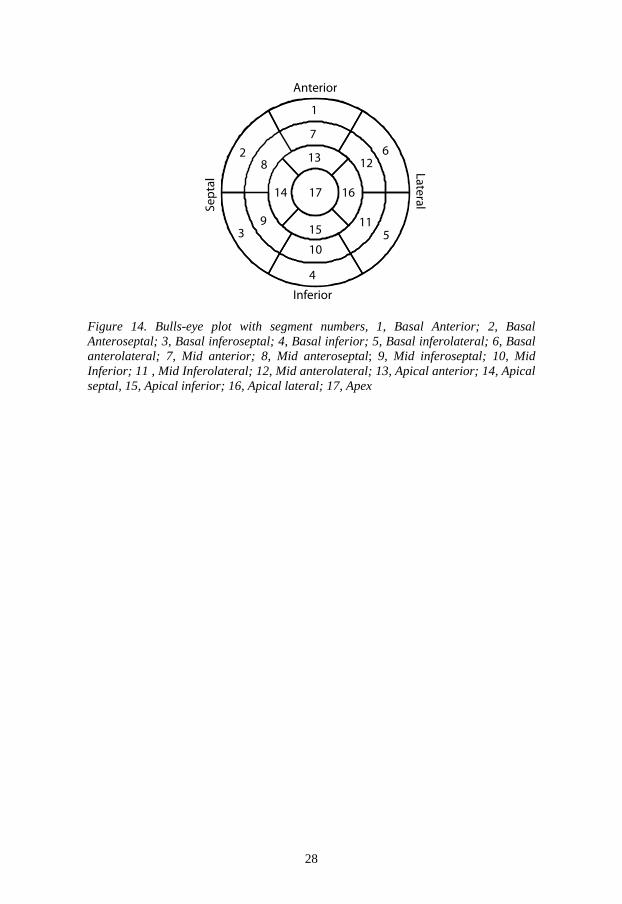
term is called the transient inertia (the time derivative), the second term is called the convective inertia (the spatial derivative), the third term is called the viscous inertia and the last term is the body forces. The latter was ignored in this study because it should be canceled out in a closed system (31). µ is the viscosity of blood (0.004 Ns/m2) and ρ is the density of blood (1060 kg/m3) (31). In order to present the data in a comprehensive way, the LV lumen was divided according to a seventeen segment model (14), which is usually applied to study the wall motion. In this study however, the segments are pie shaped instead of circular arches. The segments are presented in figure 14. Furthermore, the pressure data were converted to a file format compatible with the commercial visualization software Ensight (CEI Inc, Research Triangle Park, NC, USA) and visualized by the use of clip planes and volume renderings. Moreover, in order to assess the pressure dynamics of diastole and its sub phases, key time frames of the diastolic phase were defined from the velocity curves over the mitral and aortic valves (figure 3b). These curves were plotted from velocity data extracted from points in the aortic and mitral valves. The pressure data along a line from MV to LV apex was exported at times of half up- and down-slopes of diastolic E- and A-waves as well as at the peaks.

28

Figure 14. Bulls-eye plot with segment numbers, 1, Basal Anterior; 2, Basal Anteroseptal; 3, Basal inferoseptal; 4, Basal inferior; 5, Basal inferolateral; 6, Basal anterolateral; 7, Mid anterior; 8, Mid anteroseptal; 9, Mid inferoseptal; 10, Mid Inferior; 11 , Mid Inferolateral; 12, Mid anterolateral; 13, Apical anterior; 14, Apical septal, 15, Apical inferior; 16, Apical lateral; 17, Apex

1

2

3

4

5

67

13 12

11

10

9

8

14

15

1617

Anterior

Inferior

Sept

alLateral

29

8 Assessment of turbulent kinetic energy

In order to utilize the extension of the 4D flow MRI technique (20, 21, 24-26), and assess TKE in the LV of DCM patients, as well as healthy subjects, a tool for assessment of LV TKE was implemented. The LV was segmented at all diastolic time frames using the freely available software Segment (Medviso, Lund, Sweden) (43). The timing of ED and ES was defined as the first time frame after closure of the mitral or aortic valve, respectively. These time frames were determined from visual inspection of the three-chamber view for each subject. In order to guarantee that all blood was included, the segmentation included some myocardium: the TKE values are negligible in the myocardium and a pilot study confirmed that this approach would not impact the results to a great extent. The segmentation was used to create a binary mask that was resampled to a mesh fitting that fitted the 4D flow data (figure 15). Every voxel outside this mask was excluded.

Figure 15. A three-chamber image with an isosurface visualization of the LV segmentation used to separate the LV voxels. The TKE was integrated over the volume in order to get the TKELV, in other words, the sum of TKE for all voxels in the LV volume, for any one arbitrary time frame, calculated as:

[ ]JvolumevoxelTKETKETFatLVinvoxelsofnumber

iiLV

=

⋅=1

[eq 10]

The TKELV was also summed over all diastolic time frames. Peak TKELV was identified at E-wave and A-wave and compared between the healthy and DCM group. The peak TKELV values were compared to transmitral peak velocity and dimensions of the LV at anteroseptal-posterolateral and mitral annulus.

31

9 Results

As a first step in this thesis work, a method for analysis of LV intracardiac 4D flow data was implemented, this was validated against other modalities rendering comparable parameters. An intra- and inter-user variability study was conducted. The proposed 4D flow method was then expanded and applied to a group of healthy subjects (paper II) and to a group of DCM patients (paper III). In the two last studies, analysis tools that facilitated faster analysis and inclusion of more data sets were implemented. In study IV: a multigrid solver was used to solve the pressure Poisson equation in order to calculate the relative pressure fields in the LV of healthy subjects. Further, the data was divided according to a 17-segment model for a more comprehensive presentation. In paper V: the TKE in the LVs of DCM patients and healthy subjects were assessed.

9.1 Flow pattern quantification

Figure 16. Pathline visualization of the four flow components constituting the EDV (Direct Flow, green; Retained Inflow, yellow; Delayed Ejection Flow, blue and Residual Volume, red) in a healthy 42 year old male at time of A) Onset diastole and B) End systole. A semi-transparent three-chamber image provides anatomical orientation. LA, Left Atrium; and LV, Left Ventricle. The pathline analysis method was validated by:

i. Comparison of in- and outflow volumes (figures 16 and 17) ii. Contrasting and comparing the SVs from the pathline method to SVs from

2Dcine PC-MRI and Doppler US in the same subjects (figure 18). iii. An inter- and intra-observer variability study was conducted (figure 19).

32

The left ventricular EDV was divided into four different components (figure 16). The inflow (constituted by Direct Flow and Retained Inflow) compared to the outflow (constituted by Direct Flow and Delayed Ejection Flow) showed no significant difference in any of the three rounds the data was analyzed (figure 17).

Figure 17. Mean and std of inflow (white) and outflow (black) volumes [ml] for the nine subjects. None of the three tests rendered significant differences between inflow and outflow. I1 A1, Investigator One Analysis One; I1 A2, Investigator One Analysis Two and; I2, Investigator Two. Further, the SV from the 4D flow method has a value between the SV from Doppler US and 2Dcine PC-MRI (Figure 18). The SVs from 2Dcine PC-MRI was significantly larger than the 4D flow derived SVs (p-value=0.004). While the 4D flow derived SV was significantly larger than the SV from Doppler US (p-value=0.005) (figure 18). The inter- and intra-observer variability study showed that there were basically no differences between the three sets of analysis results. The EDV obtained from 4D flow by Investigator I, second analysis and that from Investigator II showed a borderline significance, p-value=0.01 which was the significance value (figure 19).

I1 A1 I1 A2 I20

10

20

30

40

50

60

70

80

90[m

l]

Inflow Outflow

33

Figure 18. A) The individual outflow volumes [ml] from the pathline method (* 4D Flow), 2DcinePC-MRI (Δ 2D Flow) and Doppler ultrasound (+ US). B) The group mean and std for the nine subjects for each different modality. By the use of pairwise t-tests, 4D flow was significantly smaller than 2D flow (* p-value = 0.004) and significantly larger than US († p-value = 0.005). H, healthy subject; DCM, patient with dilated cardiomyopathy.

I1A1 I1A2 I20

20

40

60

80

100

120

140

160

180

DF RI DEF REV0

5

10

15

20

25

30

35

40

45

I1 A1

I1 A2

I2

End-

dias

tolic

vol

ume

[ml]

Perc

ent o

f end

-dia

stol

ic v

olum

e

A B

Figure 19. Results from the inter- and intra-observer variability study, for each investigator and analysis. A) Mean and std of the EDV (from the nine included subjects) obtained from the 4D flow pathline method. B) Mean and std of the four flow components (DF, Direct Flow; RI, Retained Inflow; DEF, Delayed Ejection Flow; and REV Residual Volume) as a percentage of each subject’s EDV, for each of the three analysis sets. I1 A1, Investigator One Analysis One; I1 A2, Investigator One Analysis Two and; I2, Investigator Two.

9.2 Normal LV blood flow characteristics In Paper II, the EDV was successfully divided into the four different functional flow components: Direct Flow, Retained Inflow, Delayed Ejection Flow and Residual Volume (figure 20 and 21). Furthermore, the inflow components (Direct Flow and Retained Inflow) were divided into early and late inflow (figure 20 and 22).

H1 H2 H3 H4 H5 H6 DCM1 DCM2 DCM30

20

40

60

80

100

120

4D Flow 2D Flow US

4D Flow 2D Flow US0

20

40

60

80

100

Stro

ke v

olum

e [m

l]St

roke

vol

ume

[ml]

A

B

*†

34

Figure 20. The four EDV components (Direct Flow, Retained Inflow, Delayed Ejection Flow and Residual Volume) as a percentage of EDV. The two inflow components (Direct Flow and Retained Inflow) were further divided into early and late filling (represented by darker tones of green and yellow, respectively).* p < 0.01 vs. Direct Flow, † p=0.00 vs. Retained Inflow, ‡ p=0.00 vs. Delayed Ejection Flow and § p=0.00 vs. Retained Inflow Early. EDV, End-diastolic volume. The Delayed Ejection Flow component seems to reside in the basal and mid parts towards the septum side of the heart, while the Residual Volume is spread around the LV walls and towards the apical third of the LV during diastole (figure 21). The inflow components seem to separate during diastole: the Retained Inflow will be positioned on the posterior side of the LV and enter deeper towards apex while the Direct Flow will enter more basally and on the anteroseptal side. For, the full components, as well as the early and late parts of the inflow components the KE, distance, φ and the linear momentum were calculated (figure 22).

Direct (Early) 19 ± 4%

Direct (Late) 18 ± 4%

Retained (Early) 11 ± 3%

Retained (Late)

6

± 2%§

Delayed Ejection Flow 16 ± 3%*

Residual Volume 30 ± 5%*,†,‡

Direct Flow37 ± 5 %

17 ± 4 %*

EDV 143 ± 22 ml

35

Figure 21. Pathline visualization of diastolic LV flow in a healthy 50 year old female. A semi-transparent three-chamber image provides morphological orientation. Left column, early diastole; center column, diastasis and right column, atrial contraction. A-C) Inflow components: Direct Flow (green) and Retained Inflow (yellow). D-F) Components residing in the LV during diastole: Delayed Ejection Flow (blue) and Residual Volume (red). LA, Left Atrium; and LV, Left Ventricle.

36

Direct Retained Delayed Residual0

0.5

1

[mJ]

Direct Retained0

0.5

1

[mJ]

Total Early Late

Direct Retained Delayed Residual0

0.05

0.1

[m]

Direct Retained0

0.05

0.1

[m]

A B

C D

E F

G H

Direct Retained Delayed Residual0

50

100

150

200

[deg

rees

]

Direct Retained0

50

100

150

200

[deg

rees

]

Direct Retained Delayed Residual

0

1

2x 10

[kgm

/s]

Direct Retained

0

1

2x 10

[kgm

/s]

p=0.000

p=0.000 p=0.000

p=0.000 p=0.004

p=0.008 p=0.002

p=0.000

*

*†

‡

* †

*

‡

†

‡

Figure 22. The left column shows kinetic energy [J] (A), distances [m] (C), angles [degrees] (E) and linear momentum [kgm/s] (G) for the full components at time of ED. The right column shows Direct Flow and Retained Inflow, total, early and late at time of ED for the same parameters as the left column.* p ≤ 0.0251 vs. Direct Flow, † p ≤ 0.0002 vs. Retained Inflow and ‡ p≤0.006 vs. Delayed Ejection Flow. There was no significant difference between LV inflow and outflow 77 ± 17 ml vs. 77 ± 16 ml (p-value = 0.75).

9.3 Blood flow in the myopathic left ventricle In one group of ten DCM patients (table 2), the LV was segmented at times of ES and ED and the analysis from studies I and II was applied to all data sets. A group of ten healthy subjects was also included (table 1). The EDV was separated into the four components Direct Flow, Retained Inflow, Delayed Ejection Flow and Residual Volume (figure 23). The blood flow components were visualized by the use of the commercially available software Ensight (CEI Inc, Research Triangle Park, NC, USA) (figure 24). Diastolic KE was calculated for each component and normalized by the volume for each component (figure 25). Two peaks could be identified in the KE plots from inflow components, while the residing components showed lower KE and one lower peak could be identified during the E-wave.

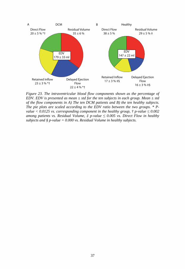
37

Direct Flow 20 ± 5 % *†

Direct Flow 38 ± 5 %

Residual Volume 35 ± 6 %

Residual Volume 29 ± 5 % ‡

Delayed EjectionFlow

16 ± 3 % ‡§

Delayed EjectionFlow

22 ± 4 % *†

EDV 179 ± 33 ml

EDV 147 ± 22 ml

DCM HealthyA B

Figure 23. The intraventricular blood flow components shown as the percentage of EDV. EDV is presented as mean ± std for the ten subjects in each group. Mean ± std of the flow components in A) The ten DCM patients and B) the ten healthy subjects. The pie plots are scaled according to the EDV ratio between the two groups. * P-value < 0.0125 vs. corresponding component in the healthy group, † p-value ≤ 0.002 among patients vs. Residual Volume, ‡ p-value ≤ 0.005 vs. Direct Flow in healthy subjects and § p-value = 0.000 vs. Residual Volume in healthy subjects.

38

Figure 24. Pathline visualization of the four EDV components: Direct Flow (green), Retained Inflow (yellow), Delayed Ejection Flow (Blue) and Residual Volume (Red). A-C) Healthy 56 year old female, D-F) 62 year old male DCM patient with relaxation abnormal diastolic filling pattern; G-I) 49 year old male DCM patient with pseudonormal diastolic filling pattern and J-L) 61 year old female with restrictive diastolic filling pattern. A morphological three-chamber image provides anatomical orientation. Ao, aorta; LA, Left Atrium; LV, Left Atrium.

39

0 50 1000

0.5

1

x 10[J

/ml]

% of EDV

DCM Patients

0 50 1000

0.5

1

x 10

[J/m

l]

% of EDV

Healthy

0 50 1000

0.5

1

x 10

[J/m

l]

% of EDV0 50 100

0

0.5

1

x 10

[J/m

l]

% of EDV

0 50 1000

0.5

1

x 10

[J/m

l]

% of EDV0 50 100

0

0.5

1

x 10

[J/m

l]

% of EDV

0 50 1000

0.5

1

x 10

[J/m

l]

% of EDV0 50 100

0

0.5

1

x 10

[J/m

l]

% of EDV

A B

C D

E F

G H

Dire

ct F

low

Del

ayed

Eje

ctio

n Fl

owRe

sidu

al V

olum

e

Figure 25. Kinetic energy per ml of blood for all subjects over the diastolic phase, normalized by the individual length of the diastolic phase. Left column shows the ten patients and right column the ten healthy subjects. A-B) Direct Flow, C-D) Retained Inflow E-F) Delayed Ejection Flow and G-H) Residual volume. The KE per ml for each component was compared at time of ED within each group as well as between the two groups (figure 26). The exchange components: Retained Inflow and Delayed Ejection Flow were higher than the Direct Flow in the patient group, while in the healthy group the Direct Flow KE was the highest.

40

Figure 26. Kinetic energy per ml of blood for each of the four components at time of ED. The left group shows data for the ten DCM patients mean ± std and the right group the corresponding values for the healthy subjects. * p-value < 0.0125 vs. the corresponding component in healthy subjects, † p-value ≤ 0.0001 vs. Direct Flow and ‡ p-value ≤ 0.0001 vs. Residual Volume, within the same group. In addition, the early and late Direct Flow as percentage of total inflow was compared. In the DCM group, the total Direct Flow as the percentage of total inflow was significantly smaller than it was in the healthy group (46+9 % vs. 70+6%, P=0.000). The Direct Flow entering during the A-wave was significantly smaller in the DCM group, as compared to the healthy group. The KE preserved at ED for the Direct Flow did not show any significant difference in the DCM group, while in the healthy group the KE from the A-wave was larger (figure 27).

Figure 27. A) Early and late Direct Flow as a percentage of the total inflow. B) The KE per ml, preserved at ED for Direct Flow. DF E, Direct Flow Early; DF A, Direct Flow Atrial contraction. * P-value = 0.000 for Direct Flow A-wave in DCM vs. healthy and † P-value = 0.003 for Direct Flow E-wave vs. Direct Flow A-wave in healthy subjects.

DCM Healthy0

0.005

0.01

0.015

0.02

0.025

[mJ/

ml]

DF

RI

DEF

ReV

*‡ *‡ *†

†‡ †‡ †

DF E DF A0

20

40

60

A

B

DCM Healthy

DF E DF A0

0.005

0.01

0.015

0.02

[mJ/

ml]

*

†

41

9.4 Left ventricular relative pressure Pressure was computed in 12 healthy subjects. Key time frames were identified based on the velocity curves over the MV and aortic valve. The pressure fields were visualized using Ensight (figure 28). The LV lumen was, at all time frames, divided according to a 17-segment model (figures 29 and 30); in order to relate different time frames to each other, the median of the apex segment (segment no 17 in figure 14) was subtracted from the median in the other 16 segments, and the data were plotted over the entire cardiac cycle (figure 29), along with the velocities at the aortic and mitral valves. The median and range of each of the 16 segments relative the apical segment for the 12 healthy subjects are presented in figure 30. At time of downslopes of E-wave all segments had significantly smaller values compared to the corresponding time of A-wave. Furthermore, pressure data along a line from MV to LV apex was extracted from all subjects at times of: upslope, peak and downslope of the E- and A-waves (figure 31). The up- and downslopes showed similar patterns, while the peak curves differed more.

Figure 28. Visualization of atrioventricular pressure maps at times of A) upslope of the E-wave, B) downslope of the E-wave, C) upslope of the A-wave and D) downslope of the A-wave. NB: the gradients are shifted. LA, Left Atrium; LV, Left Ventricle.

42

2.5

1.5

0.5

0

0.5

1

1.5

0 0.2 0.4 0.6 0.8 10

0.2

0.4

0.6

2.5

1.5

0.5

0

0.5

1

1.5

0 0.2 0.4 0.6 0.8 10

0.2

0.4

0.6

2.5

1.5

0.5

0

0.5

1

1.5

0 0.2 0.4 0.6 0.8 10

0.2

0.4

0.6

2.5

1.5

0.5

0

0.5

1

1.5

0 0.2 0.4 0.6 0.8 10

0.2

0.4

0.6

2.5

1.5

0.5

0

0.5

1

1.5

0 0.2 0.4 0.6 0.8 10

0.2

0.4

0.6

2.5

1.5

0.5

0

0.5

1

1.5

0 0.2 0.4 0.6 0.8 10

0.2

0.4

0.6

Time [s]

Time [s]Time [s]

Time [s]Time [s]

Time [s]

[mm

Hg]

[mm

Hg]

[mm

Hg]

[m/s]

[ m/s]

[ m/s]

[mm

Hg]

[mm

Hg]

[mm

Hg]

[m/s]

[ m/s]

[m/s]

A

C

B

D

F

E

2.5

1.5

0.5

0

0.5

1

1.5

0 0.2 0.4 0.6 0.8 10

0.2

0.4

0.6

Time [s]

[mm

Hg]

[m/s]

H

2.5

1.5

0.5

0

0.5

1

1.5

0 0.2 0.4 0.6 0.8 10

0.2

0.4

0.6

Time [s]

[mm

Hg]

[m/s]

G

2.5

1.5

0.5

0

0.5

1

1.5

0 0.2 0.4 0.6 0.8 10

0.2

0.4

0.6

Time [s]

[m/s]

[mm

Hg]

I

2.5

1.5

0.5

0

0.5

1

1.5

0 0.2 0.4 0.6 0.8 10

0.2

0.4

0.6

Time [s]

[mm

Hg]

[m/s]

J

2.5

1.5

0.5

0

0.5

1

1.5

0 0.2 0.4 0.6 0.8 10

0.2

0.4

0.6

Time [s]

[mm

Hg]

[m/s]

K

2.5

1.5

0.5

0

0.5

1

1.5

0 0.2 0.4 0.6 0.8 10

0.2

0.4

0.6

Time [s]

[mm

Hg]

[m/s]

L

Figure 29. Pressure relative to the apical segment in 16 segments over the cardiac cycle for all subjects. Left y-axis: Median pressure [mmHg] in each segment relative to the median pressure in the apical segment over time [s]. Right y-axis: Velocity [m/s] over time [s] at position of the mitral valve. All twelve healthy subjects are represented (A-L). Pressures from basal segments (segments 1 through 6) are shown in black, mid segments (7 through 12) in blue and apical segments (13 through 16) in red.

43

(0.74)

(1.0

8) *†

(0.95)

(1.06)*(0

.97)

*

(0.78)*

(0.68)*

(0.7

8)*

(0.93)*

(0.85)*

(0.7

4)

(0.67)*

(0.48)

(0.3

9)†

(0.52)

(0.5

4)

0.00

(0.49)

(0.6

9)†

(0.71)(0.53)

(0.4

4)

(0.44)(0.34)

(0.3

4)

(0.30)(0.29)

(0.3

2)

(0.37)(0.13)

(0.1

2)

(0.12)

(0.1

7)0.00

E-wave A-waveA B

Figure 30. Bull’s-eye plots showing the median of the median pressure relative to the apex and the range of medians in the 12 healthy subjects at half of the downslope of the E-wave (A) and A-wave (B). * p-value < 0.0031 same segment number E-wave vs. A-wave. † p-value < 0.0056 same time frame SA comparisons. Antero-septal and infero-lateral long-axis comparisons all gave a p-value < 0.0005.

44

Figure 31. Pressure [mmHg] relative to apex along a line from mitral valve (MV) to apex at time of A) upslope of E- and A-waves, respectively, B) peak of E- and A-waves and C) downslope of E- and A-waves. Note the similar patterns at upslope and downslope while the peak E- and A-waves seems to differ more.

0 0.2 0.4 0.6 0.8 1

0

0.5

1

Relative distance from MV

[mm

Hg]

E waveA wave

0 0.2 0.4 0.6 0.8 1

0

0.5

1

Relative distance from MV

[mm

Hg]

E waveA wave

0 0.2 0.4 0.6 0.8 1

0

0.5

1

Relative distance from MV

[mm

Hg]

E waveA wave

Half upslope

Peak

Half downslope

A

B

C

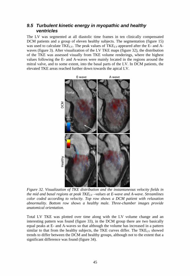
45

9.5 Turbulent kinetic energy in myopathic and healthy ventricles

The LV was segmented at all diastolic time frames in ten clinically compensated DCM patients and a group of eleven healthy subjects. The segmentation (figure 15) was used to calculate TKELV. The peak values of TKELV

appeared after the E- and A- waves (figure 3). After visualization of the LV TKE maps (figure 32), the distribution of the TKE was assessed visually from TKE volume renderings, where the highest values following the E- and A-waves were mainly located in the regions around the mitral valve, and to some extent, into the basal parts of the LV. In DCM patients, the elevated TKE areas reached further down towards the apical LV.

Figure 32. Visualization of TKE distribution and the instantaneous velocity fields in the mid and basal regions at peak TKELV –values at E-wave and A-wave. Streamlines color coded according to velocity. Top row shows a DCM patient with relaxation abnormality. Bottom row shows a healthy male. Three-chamber images provide anatomical orientation. Total LV TKE was plotted over time along with the LV volume change and an interesting pattern was found (figure 33), in the DCM group there are two basically equal peaks at E- and A-waves so that although the volume has increased in a pattern similar to that from the healthy subjects, the TKE curves differ. The TKELV showed trends to differ between the DCM and healthy groups, although not to the extent that a significant difference was found (figure 34).

46

0% 50% 100%

0

1

2

3

4T

KE

[mJ]

Percentage of Diastole0% 50% 100%

0

100

LV V

olum

e C

hang

e [m

l]

0% 50% 100%

0

1

2

3

4

TK

E [m

J]

Percentage of Diastole0% 50% 100%

0

100

LV V

olum

e C

hang

e [m

l]

A BDCM Healthy

Figure 33. TKE total (blue) and LV volume change over diastole (red) (mean ± std) for DCM patients (left panel) and healthy subjects (right panel).

Figure 34. Mean and std of peak TKELV at early (E) and late (A) diastolic filling, for the eleven healthy subjects and the ten DCM patients.

0

0.5

1

1.5

2

2.5

3

3.5

4

4.5

5x 10

DCM Healthy

TK

E [J]

47

10 Discussion

When the MRI examination is finished and the patient has left the scanner, the thousands of heartbeats, each partially stored as lines of k-space data are processed, and reconstructed into one single cardiac cycle and then exported from the scanner for further processing offline. The CMR group at Linköping University has been working for over a decade on both acquisition and postprocessing. This thesis includes studies aiming to bring the 4D flow MRI technique closer to the clinical setting. In this thesis, methods for analysis and applications of these have been presented in the underlying studies. Cardiac 4D flow applications to the full cardiac cycle have been lacking over the years, the reason being that only one vendor has implemented a retrospective cardiac gating in the scanner software for 4D flow sequences, which we have used in this work. Prospectively gated sequences do not allow reconstruction of the full cardiac cycle; about 80-90 percent of the cardiac cycle is reconstructed (39, 61). Despite this some cardiac applications have been published using these sequences (60). The VIPR sequence, first applied to brain vessels have shown potential to provide cardiac 4D flow data with high resolution (40, 47).

10.1 Studying cardiovascular blood flow using 4D flow MRI Over the last century, technical advancements have been extreme, which has led to development at all levels in society. Though, assessments of cardiovascular velocity fields are not as old. Blood flow measurements using US were first presented in the 1960s (81). In 1982, Moran presented a work about measuring blood flow velocities using MRI (70). As a consequence of the advances in technique, different modalities such as US, MRI and CFD have given us a deeper insight into cardiovascular physiology and blood flow. Prior to these advances, the only available flow measurements were invasive measurements, using as e.g. pressure catheters and thermo dilution. Velocity measurements with MRI were initially mainly used to obtain the through plane velocity for assessment of volume flow through a vessel. Later the in-plane or sometimes three components of the velocity vector were measured in a 2D plane. A qualitative study, assessing flow properties in the heart from slices of flow data concluded that the asymmetry of the heart saves energy over time by preserving the linear momentum of the blood flow (54). This was later challenged in a numerical model (94), studying LV blood flow in a healthy subject and a DCM patient with a single leaflet mechanical valve, changing the direction of the inflow and reversing the central LV vortex. The hypothesis that the asymmetric heart would conserve energy by conserving momentum was tested and the conclusion was that the heart does not save energy by conserving momentum. This led to some debate regarding the definition of a looped heart (52, 95). Kim (55), assessed vortex formation and vortical kinetic energy from a three-directional, two-dimensional acquisition in a group of 26 healthy subjects. Their KE findings were approximately a

48

factor of five lower than ours, which might be explained by the fact that they assessed vortical KE in a 2D slice. Mohiaddin (68) presented a study with streamline visualization in a group of dilated cardiomypathy patients. Data were obtained from a three-chamber view, describing the larger mid ventricular vortex in the LV in the DCM patients. These findings are also supported by our data. The first full 4D flow MRI sequence was presented at a conference proceeding in 1993 (34). Later, in 1996, another sequence was presented in a full length paper (97), this technique proved to hold potential for pathline visualization of atrioventricular blood flow patterns over a full cardiac cycle (96). LA blood flow characteristics were assessed by the use of streamlines and pathlines, where propagation time and size of vortices were measured and the path from different pulmonary veins was calculated and related to the absolute distance between pulmonary vein and mitral valve. In this early study, not only were pathlines and streamlines used for visualization, they were used for quantification as well (38). Later others have used the technique to estimate e.g. KE. Carlsson et al (13) segmented the LV and RV and calculated kinetic energy from the velocity over the cardiac cycle. Arvidsson et al (3) segmented the LA and RA and calculated the KE over the cardiac cycle. The magnitude of their KE findings were in the same range as in paper II presented in this thesis. Vortical structures in the flow in the different chambers of the heart have been attributed several important functions, e.g. aiding valve opening (15) and closure. Different methods and approaches have been applied to assess the vortical flow in the different heart chambers (51), including automatic vortex detection techniques (42). Besides 4D flow MRI, echocardiographic particle image velocimetry (PIV) has been used to assess the vortical nature of LV flow (46, 50). Lagrangian coherent structures were used to assess the volume of the mitral vortex ring (93).

10.2 Flow component studies using other approaches Bolger et al. (8) presented a study where the EDV in healthy subjects was divided into the four components Direct Flow, Retained Inflow, Delayed Ejection Flow and Residual Volume; their results differed in some aspects from the ones in papers I-III. This may be due to several factors, the MRI data were acquired on a different system, with different parameters, the data were acquired without respiratory gating, risking that the data is more smeared. The temporal and spatial resolution and the analysis method were also different. But probably most important, the analysis approach used in this thesis is less prone to errors. Hendabadi et al. (44) applied our definition of the four flow components to the LV using bi-directional velocity field maps acquired using US combined with trajectory-based computation of lagrangian coherent structures. Their study resulted in a slightly higher relative Direct Flow than in the healthy subjects and patients in our studies, but there is fairly good agreement; the ratio of total inflow that Direct Inflow constitutes agreed fairly well as well. They assessed the exchange of the Residual Volume as well. Mangual et al (59) used 3D echo to acquire the anatomy of the heart in order to have anatomical input data for simulations. Their findings were more in line with those from Bolger et al (8). Simulations may provide important information, although several assumptions underlie a simulation, which make cardiac simulations extremely difficult and computationally demanding. Fredriksson et al (35), applied the method presented in papers I and II, on the RV in healthy subjects, describing the distribution regarding the four components of the EDV of the right ventricle, they found that the

49

EDV was slightly smaller, while the Direct Flow as a percentage of the EDV was significantly larger and the Residual Volume was significantly smaller. In severely dilated LVs with low EFs, the Residual Volume represents a large part of the EDV, so even if the LV volume is large “the functional ventricle”, i.e. the areas where exchange occur, is a lot smaller than in the healthy ventricle and the rest is “padded” with Residual Volume (12). Maze et al (66) studied the LV flow characteristics in a group of DCM patients with and a group without LV thrombus. They assessed ventricular velocities with Doppler ultrasound and found that velocities were lower or even lacking in the apical regions of the LV in the thrombus prone group. When this study was published no other method of assessing apical flow was available. However, with the method used in papers I-III, this would be possible to assess. Furthermore, Maze et al, pointed out that, although the phenomenon was observable, they could not determine whether it was the cause of the thrombus formation or a consequence of it. Watanabe and colleagues stated that blood flow in the heart follows a first in first out principle (94). This has not been observed in the papers underlying this thesis. When dividing components into early and late inflow it appears that the Direct Flow entering early and late will leave at approximately the same time. This is also in line with the findings from Bolger et al (8) who also looked at early and late inflow.

10.3 Accuracy of pathlines Papers I-III are based on the use of pathlines. When integrating pathlines, truncation errors due to spatial and temporal interpolation, and offsets in velocity data will progress and add over time. Too low spatial and temporal resolution will also make pathlines stray off from the actual path. Hence, the certainty of a pathline will decrease the longer it is integrated (36, 37). Probability maps from an aortic data set were generated. Pathlines were emitted from the same points and the data was changed according to a Monte Carlo model (36, 37). Darmofal and Haimes (19) evaluated several algorithms for calculation of pathlines, they assumed that the only interpolation needed was temporal and one of the algorithms they evaluated was the fourth order Runge-Kutta algorithm that utilized by Ensight (1, 19). Their conclusion was that this algorithm as well as several other algorithms provides accurate pathlines. One advantage with the approach chosen in papers I-III is that the pathlines are not calculated for one full cardiac cycle at once, they are emitted at time of ED and calculated for systole and diastole separately. This ensures that components that end up outside the LV will spend the end time, i.e. the most uncertain time outside the LV. Most of the numerical comparisons are from ED, which is the first time frame that the pathlines are emitted from: this should minimize the effect of summed errors. LV in- and out-flow should be equal and the EDV should be close to that from the EDV obtained from the segmentation of the SA-axis images. Furthermore, LV in-flow and out-flow should be equal to stroke volume estimates obtained from other methods, like volume flow measurements from velocity measurements in ascending aorta, as shown in paper I. This can be used to detect low quality datasets. This pathline method has been used for quality control of 4D flow data, when testing different settings and new sequences. Visualization of the components has the potential to reveal drift due to velocity offsets and noise.

50

10.4 Turbulent kinetic energy There are only a few studies utilizing MRI rendered TKE-data in the heart. Dyverfeldt et al. (23), looked at a group of five patients with mitral valve prolapse of the middle scallop, they found a linear correlation between TKE values and regurgitant volume. Otherwise, TKE studies in the current literature have presented aortic flow. Simulations of TKE in a patient with aortic coarctation have been carried out (4). Dyverfeldt el al studied the relation between pressure drop through a stenotic aortic valve and TKE (22). In an attempt to assess disturbed blood flow in the aorta the Reynolds number has been examined, based on velocities and the aortic geometry from MRI (84).

10.5 Pressure So far there have not been many studies presented concerning LV relative pressure fields calculated from 4D flow data; in (31) one healthy subject was included presenting the feasibility of relative pressure fields. Our data seem to be consistent with this subject in terms of pressure range and general characteristics, such as minimum and maximum value distribution. Buyens et al used acceleration encoded MRI data to assess left ventricular pressure (11). Vascular applications have mainly focused on the aorta (7, 57, 91, 101) although other applications exist as well e.g. (67). Elevated turbulence intensity, i.e. elevated values of TKE, will render energy losses from the flow, as TKE dissipated into heat. A coarctation or a stenotic valve is a region with higher probability of elevated turbulence intensity. In such a constriction, the velocity will increase and the pressure will decrease, and, as the path widens again, the velocity decreases and the pressure will increase. However, if the flow has transitioned from laminar to disturbed flow, energy losses will cause decreased pressure recovery. In order to compensate for such losses, the pump will have to work harder to maintain pressure in the areas downstream of the flow impeding structure. The measured velocity in a regular 4D flow MRI acquisition is the mean velocity for each voxel. When using the pressure Poisson equation with MRI data, the pressure will be accurate as long as the fluctuating part is small. As the fluctuating component increases, the accuracy will decrease as this part is omitted from the calculations. The resolution is too poor to resolve all the scales of disturbed flow. Fully developed turbulence is not likely to appear in the cardiovascular system. In turbulent and disturbed flow, vortices break down into smaller and smaller vortices that, in the end, dissolve and their kinetic energy are lost as viscous dissipation. The TKE levels in paper V should not be so high that they hamper the pressure calculation in paper IV.

10.6 Limitations and future work In the studies underlying this thesis, analysis methods have been implemented and applied to both a healthy population and a DCM patient population. The studies have gone all the way from development of analysis tools to their application, in an effort to bring the 4D flow acquisition technique closer to larger studies and ultimately to the clinical setting. Although this work has brought this aim closer, much still remains to be done in virtually all of the steps. Faster data acquisition is needed; which was outside of the scope of this thesis. Promising progress has been shown with spiral k-space readouts (82). Data acquisitions in patients with stenotic or otherwise insufficient valves can also be challenging, due to the wide range of the velocity distribution and one solution may be the use of dual VENC sequences (48, 72).

51

Faster reconstruction on the scanner, the possibility of automatic segmentation on the 4D flow data directly, or as a step on the way, co-registration of the morphological images to the 4D flow data are also areas in need of improvement. The method used in papers I-III has been using pathlines calculated in Ensight, although now a faster approach has been implemented, where the pathlines are calculated directly in the analysis software, lowering the analysis time by approximately ten minutes. One limitation is the segmentation part of the analysis in all papers presented in this thesis, relying on data from another data acquisition results in uncertainty. Attempts to segment the 4D flow data directly have been made (27), but contrast of the signal magnitude of the 4D flow MRI has, so far, been too poor (figure 35). With other acquisitions and improvement in hardware, segmentation of the 4D flow data directly may be possible in the future. In the studies underlying this thesis, the challenge of mismatch between data sets was addressed by acquiring one stack of SA-images before 4D flow data and one SA-stack after. This approach gives the possibility of assessing whether the subject moved during the examination and of selecting the SA-stack which shows the best fit. An improved approach for segmentation of 4D flow data or registration of 4D flow data and morphological data are thus a prerequisite of future studies. A larger inter- and intra-observer variability study should be undertaken, with blinded analysis of the data sets and perhaps even different segmentation approaches. Inter vendor studies are also needed to compare vendor and site variability and to establish normal material.

Figure 35. Top row show morphological bSSFP images, bottom row show the same view in a cut plane from the magnitude data of the 4D flow data. Left column show a three-chamber view; and right column show short-axis view in the mid of the LV. The black line crossing the SA-image shows where the three-chamber plane crosses the SA-image. NB that the full RV is not included in the 4D flow data. Hence, the black band at the top of that image. Note the poor contrast between myocardium and blood pool, in the 4D flow magnitude. LV, Left Ventricle; LA, Left Atrium; RV, Right Ventricle.

52

10.7 Potential impact This thesis shows that 4D flow data can be used to present quantitative results from 4D flow data that may add to the understanding of both normal physiology and pathophysiology. It presents streamlined analysis methods, which could, in time, be used in the clinical setting. LV blood flow patterns from patients more prone to thrombus should be further assessed. Furthermore, the pressure data can be used to assess patients with regional wall motion abnormalities and hypertrophic ventricles.

53

11 Conclusion

In this thesis a semi-automatic approach, for quantification and visualization of intracardiac blood flow patterns was developed. Furthermore, this method facilitates the evaluation of intra cardiac 4D flow MRI data quality and eliminates some user dependent steps from previous methods. Using this approach, new insight into blood flow patterns in the healthy, as well as the myopathic, left ventricle was obtained. Further insight into intra cardiac blood flow dynamics was obtained by assessment of the distribution of relative pressure fields in healthy left ventricles. The used method is applicable to a larger amount of data sets and is also a way to present the data in a more comprehensive manner. Assessment of turbulent kinetic energy in the left ventricle showed increased values in the diseased, as compared to the healthy. The methods and applications presented in this thesis facilitate quantification and visualization of intra cardiac blood flow dynamics, leading to enhanced understanding of normal physiology, as well as pathophysiology, ultimately bringing 4D flow data closer to the clinical setting.

55

12 Acknowledgments

The thesis work has been undertaken at the Division of Cardiovascular Medicine at the Department of Medical and Health Sciences and at the Center for Medical Image Science and Visualization (CMIV). During all the hours behind the studies, as well as the writing of this thesis, I have had the privilege and honor to be surrounded by great and inspiring persons. I would like to express my sincere gratitude to each of these persons. First of all I would like to acknowledge my supervisor Tino Ebbers, who gave me the opportunity to go through the PhD studies, inspired and encouraged me and shared his knowledge in the MRI technique, method development and scientific methodology. Further, I would like to acknowledge Carl-Johan Carlhäll, my co-supervisor, for inspiration and support and for sharing his insights into physiology, pathophysiology and research methodology as well as for showing the focus and discipline needed to produce good research. Ann Bolger is a never ending source of ideas and inspiration and has had a large impact on this work, thank you. Jan Engvall has given valuable input and support in questions regarding physiology and clinical routine. John-Peder Escobar Kvitting has discussed and shown me parts of the world of thoracic surgery. Thank you Matts Karlsson, for valuable input. Thanks to Petter Dyverfeldt, Henrik Haraldsson and Andreas Sigfridsson for good input, discussions and support throughout the years. I would like to extend my thanks to other past and present members of the cardiovascular MR group, Jakub Zajac, Alexandru Grigorescu Fredriksson, Jonas Lantz, Mariana Bustamante, Belén Garcia Casas and Sofia Kvernby. Sven Petersson and I started our master thesis projects at the same time and have since been working parallel on our PhD projects, thank you for good discussions, input and ideas. Thanks to Johan Kihlberg for support regarding MRI data acquisition and data export. Thanks to Eva Nylander for valuable input and Lena Forsberg and Kristoffer Hedman for several interesting discussions. Thank you, Elin Wistrand for always being helpful and finding solutions to administrative problems large and small. Thanks to everyone at CMIV and Division of Cardiovascular Medicine. Thanks to all of my friends who have given me a lot of joy and support over the years Elin, Trevor, Malin, Kristofer, Linnéa, Jennifer and Per, who also had the unfortunate task to read and give feedback on an early draft of this thesis. I would like to acknowledge my family; especially, my mother Susann, my father Leif and my brother Rikard and his girlfriend Rosanna, for continuous support and love no matter what paths in life I have chosen to tread. Thank you Sanna, for patience, support and love and for cheering me up during heavy moments. I’m looking forward to exploring the future together.

Jonatan Eriksson Linköping, October 2013

57

13 Bibliography

1. EnSight User Manual for version 10.0. 2. Report of the WHO/ISFC task force on the definition and classification of

cardiomyopathies. Br Heart J 44: 672-673, 1980. 3. Arvidsson PM, Töger J, Heiberg E, Carlsson M, and Arheden H.

Quantification of left and right atrial kinetic energy using four-dimensional intracardiac magnetic resonance imaging flow measurements. Journal of Applied Physiology 114: 1472-1481, 2013.

4. Arzani A, Dyverfeldt P, Ebbers T, and Shadden SC. In vivo validation of numerical prediction for turbulence intensity in an aortic coarctation. Annals of biomedical engineering 40: 860-870, 2012.

5. Atkins P, and De Paula J. Atkins physical chemistry. In: Seventh Ed Oxford University Press, 2002.

6. Blom G, Enger J, Englund G, Grandell J, and Holst L. Sannolikhetsteori och statistikteori med tillämpningar. 2005.

7. Bock J, Frydrychowicz A, Lorenz R, Hirtler D, Barker AJ, Johnson KM, et al. In vivo noninvasive 4D pressure difference mapping in the human aorta: phantom comparison and application in healthy volunteers and patients. Magnetic Resonance in Medicine 66: 1079-1088, 2011.

8. Bolger AF, Heiberg E, Karlsson M, Wigström L, Engvall J, Sigfridsson A, et al. Transit of blood flow through the human left ventricle mapped by cardiovascular magnetic resonance. J Cardiovasc Magn Reson 9: 741-747, 2007.

9. Boron WF, and Boulpaep EL. Medical Physiology. Elsevier Health Sciences, 2003.

10. Buonocore MH. Visualizing blood flow patterns using streamlines, arrows, and particle paths. Magn Reson Med 40: 210-226, 1998.

11. Buyens F, Jolivet O, Cesare AD, Bittoun J, Herment A, Tasu JP, et al. Calculation of left ventricle relative pressure distribution in MRI using acceleration data. Magnetic Resonance in Medicine 53: 877-884, 2005.

12. Carlhäll CJ, and Bolger A. Passing strange: Flow in the failing ventricle. Circ Heart Fail 3: 326-331, 2010.

13. Carlsson M, Heiberg E, Töger J, and Arheden H. Quantification of left and right ventricular kinetic energy using four-dimensional intracardiac magnetic resonance imaging flow measurements. American Journal of Physiology-Heart and Circulatory Physiology 302: H893-H900, 2012.

14. Cerqueira MD, Weissman NJ, Dilsizian V, Jacobs AK, Kaul S, Laskey WK, et al. Standardized myocardial segmentation and nomenclature for tomographic imaging of the heart a statement for healthcare professionals from the cardiac imaging committee of the Council on Clinical Cardiology of the American Heart Association. Circulation 105: 539-542, 2002.

58

15. Charonko JJ, Kumar R, Stewart K, Little WC, and Vlachos PP. Vortices formed on the mitral valve tips aid normal left ventricular filling. Ann Biomed Eng 41: 1049-1061, 2013.

16. Cohn JN, Ferrari R, and Sharpe N. Cardiac remodeling--concepts and clinical implications: A consensus paper from an international forum on cardiac remodeling. J Am Coll Cardiol 35: 569-582, 2000.

17. Courtois M, Kovacs Jr SJ, and Ludbrook P. Transmitral pressure-flow velocity relation. Importance of regional pressure gradients in the left ventricle during diastole. Circulation 78: 661-671, 1988.

18. Curran-Everett D, and Benos DJ. Guidelines for reporting statistics in journals published by the American Physiological Society. American Journal of Physiology - Heart and Circulatory Physiology 287: H447-H449, 2004.

19. Darmofal DL, and Haimes R. An analysis of 3D particle path integration algorithms Journal of Computational Physics 123: 182-195, 1996.

20. Dyverfeldt P. Extending MRI to the Quantification of Turbulence Intensity. Linköping, 2010.

21. Dyverfeldt P, Gårdhagen R, Sigfridsson A, Karlsson M, and Ebbers T. On MRI turbulence quantification. Magnetic resonance imaging 27: 913-922, 2009.

22. Dyverfeldt P, Hope MD, Tseng EE, and Saloner D. Magnetic Resonance Measurement of Turbulent Kinetic Energy for the Estimation of Irreversible Pressure Loss in Aortic Stenosis. JACC: Cardiovascular Imaging 6: 64-71.

23. Dyverfeldt P, Kvitting J-PE, Carlhäll CJ, Boano G, Sigfridsson A, Hermansson U, et al. Hemodynamic aspects of mitral regurgitation assessed by generalized phase-contrast MRI. Journal of Magnetic Resonance Imaging 33: 582-588.

24. Dyverfeldt P, Kvitting JP, Sigfridsson A, Engvall J, Bolger AF, and Ebbers T. Assessment of fluctuating velocities in disturbed cardiovascular blood flow: in vivo feasibility of generalized phase-contrast MRI. J Magn Reson Imaging 28: 655-663, 2008.

25. Dyverfeldt P, Sigfridsson A, Knutsson H, and Ebbers T. A novel MRI framework for the quantification of any moment of arbitrary velocity distributions. Magnetic Resonance in Medicine 65: 725-731.

26. Dyverfeldt P, Sigfridsson A, Kvitting JP, and Ebbers T. Quantification of intravoxel velocity standard deviation and turbulence intensity by generalizing phase-contrast MRI. Magn Reson Med 56: 850-858, 2006.

27. Ebbers T. Cardiovascular fluid dynamics: methods for flow and pressure field analysis from magnetic resonance imaging. 2001.

28. Ebbers T. Flow Imaging: Cardiac Applications of 3D Cine Phase-Contrast MRI. Current Cardiovascular Imaging Reports 1-7, 2011.

29. Ebbers T, and Farnebäck G. Improving computation of cardiovascular relative pressure fields from velocity MRI. Journal of Magnetic Resonance Imaging 30: 54-61, 2009.

30. Ebbers T, Haraldsson H, Dyverfeldt P, Sigfridsson A, Warntjes MJB, and Wigström L. Higher order weighted least-squares phase offset correction for improved accuracy in phase-contrast MRI. In: Proc Intl Soc Mag Reson Med 16, 2008.

31. Ebbers T, Wigström L, Bolger AF, Wranne B, and Karlsson M. Noninvasive measurement of time-varying three-dimensional relative pressure fields within the human heart. J Biomech Eng 124: 288-293, 2002.

59

32. Elliott P. The 2006 American Heart Association classification of cardiomyopathies is not the gold standard. Circulation: Heart Failure 1: 77-80, 2008.

33. Elliott P, Andersson B, Arbustini E, Bilinska Z, Cecchi F, Charron P, et al. Classification of the cardiomyopathies: a position statement from the European Society Of Cardiology Working Group on Myocardial and Pericardial Diseases. European heart journal 29: 270-276, 2008.

34. Firmin D, Gatehouse P, Konrad J, Yang G, Kilner P, and Longmore D. Rapid 7-dimensional imaging of pulsatile flow. In: Computers in Cardiology 1993, ProceedingsIEEE, 1993, p. 353-356.

35. Fredriksson AG, Zajac J, Eriksson J, Dyverfeldt P, Bolger AF, Ebbers T, et al. 4-D blood flow in the human right ventricle. Am J Physiol Heart Circ Physiol 301: H2344-2350, 2011.

36. Friman O, Hennemuth A, Harloff A, Bock J, Markl M, and Peitgen HO. Probabilistic 4D blood flow mapping. Med Image Comput Comput Assist Interv 13: 416-423.

37. Friman O, Hennemuth A, Harloff A, Bock J, Markl M, and Peitgen HO. Probabilistic 4D blood flow tracking and uncertainty estimation. Med Image Anal 15: 720-728, 2011.

38. Fyrenius A, Wigström L, Ebbers T, Karlsson M, Engvall J, and Bolger AF. Three dimensional flow in the human left atrium. Heart 86: 448-455, 2001.

39. Föll D, Taeger S, Bode C, Jung B, and Markl M. Age, gender, blood pressure, and ventricular geometry influence normal 3D blood flow characteristics in the left heart. European Heart Journal Cardiovascular Imaging 14: 366-373, 2013.

40. Gu T, Korosec FR, Block WF, Fain SB, Turk Q, Lum D, et al. PC VIPR: a high-speed 3D phase-contrast method for flow quantification and high-resolution angiography. American journal of neuroradiology 26: 743-749, 2005.

41. Hannon RA, Pooler C, and Porth C. Porth pathophysiology: concepts of altered health states. Wolters Kluwer Health, 2009.

42. Heiberg E, Ebbers T, Wigström L, and Karlsson M. Three-dimensional flow characterization using vector pattern matching. Visualization and Computer Graphics, IEEE Transactions on 9: 313-319, 2003.

43. Heiberg E, Sjögren J, Ugander M, Carlsson M, Engblom H, and Arheden H. Design and validation of Segment--freely available software for cardiovascular image analysis. BMC Med Imaging 10: 1, 2010.

44. Hendabadi S, Bermejo J, Benito Y, Yotti R, Fernández-Avilés F, del Álamo JC, et al. Topology of Blood Transport in the Human Left Ventricle by Novel Processing of Doppler Echocardiography. Annals of biomedical engineering 1-14, 2013.

45. Hill JA, and Olson EN. Cardiac plasticity. N Engl J Med 358: 1370-1380, 2008.

46. Hong GR, Pedrizzetti G, Tonti G, Li P, Wei Z, Kim JK, et al. Characterization and quantification of vortex flow in the human left ventricle by contrast echocardiography using vector particle image velocimetry. JACC Cardiovasc Imaging 1: 705-717, 2008.

60

47. Johnson KM, Lum DP, Turski PA, Block WF, Mistretta CA, and Wieben O. Improved 3D phase contrast MRI with off-resonance corrected dual echo VIPR. Magnetic Resonance in Medicine 60: 1329-1336, 2008.

48. Johnson KM, and Markl M. Improved SNR in phase contrast velocimetry with five-point balanced flow encoding. Magnetic Resonance in Medicine 63: 349-355.

49. Kameneva MV, Burgreen GW, Kono K, Repko B, Antaki JF, and Umezu M. Effects of turbulent stresses upon mechanical hemolysis: experimental and computational analysis. ASAIO journal 50: 418-423, 2004.

50. Kheradvar A, Houle H, Pedrizzetti G, Tonti G, Belcik T, Ashraf M, et al. Echocardiographic particle image velocimetry: a novel technique for quantification of left ventricular blood vorticity pattern. J Am Soc Echocardiogr 23: 86-94, 2010.

51. Kheradvar A, and Pedrizzetti G. Vortex formation in the cardiovascular system. Springer, 2012.

52. Kilner PJ. Letter to the editor: "Postulated functional advantages of a looped as opposed to a linearly arranged heart". Am J Physiol Heart Circ Physiol 298: H726; author reply H727, 2010.

53. Kilner PJ, Henein MY, and Gibson DG. Our tortuous heart in dynamic mode--an echocardiographic study of mitral flow and movement in exercising subjects. Heart Vessels 12: 103-110, 1997.

54. Kilner PJ, Yang GZ, Wilkes AJ, Mohiaddin RH, Firmin DN, and Yacoub MH. Asymmetric redirection of flow through the heart. Nature 404: 759-761, 2000.

55. Kim WY, Walker PG, Pedersen EM, Poulsen JK, Oyre S, Houlind K, et al. Left ventricular blood flow patterns in normal subjects: a quantitative analysis by three-dimensional magnetic resonance velocity mapping. J Am Coll Cardiol 26: 224-238, 1995.

56. Kirkwood BR. Essentials of medical statistics. Blackwell Scientific Publications, 1988.

57. Krittian S, Lamata P, Michler C, Nordsletten DA, Bock J, Bradley CP, et al. A finite-element approach to the direct computation of relative cardiovascular pressure from time-resolved MR velocity data. Medical Image Analysis 16: 1029-1037, 2012.

58. Kvitting J-PE, Dyverfeldt P, Sigfridsson A, Franzén S, Wigström L, Bolger AF, et al. In vitro assessment of flow patterns and turbulence intensity in prosthetic heart valves using generalized phase-contrast MRI. Journal of Magnetic Resonance Imaging 31: 1075-1080, 2010.

59. Mangual JO, Kraigher-Krainer E, De Luca A, Toncelli L, Shah A, Solomon S, et al. Comparative numerical study on left ventricular fluid dynamics after dilated cardiomyopathy. Journal of biomechanics 46: 1611-1617, 2013.

60. Markl M, Geiger J, Arnold R, Stroh A, Damjanovic D, Föll D, et al. Comprehensive 4-dimensional magnetic resonance flow analysis after successful heart transplantation resolves controversial intraoperative findings and reveals complex hemodynamic alterations. Circulation 123: e381-e383.

61. Markl M, Harloff A, Bley TA, Zaitsev M, Jung B, Weigang E, et al. Time-resolved 3D MR velocity mapping at 3T: Improved navigator-gated assessment of vascular anatomy and blood flow. Journal of Magnetic Resonance Imaging 25: 824-831, 2007.

61

62. Markl M, Kilner PJ, and Ebbers T. Comprehensive 4D velocity mapping of the heart and great vessels by cardiovascular magnetic resonance. Journal of Cardiovascular Magnetic Resonance 13: 1-22, 2011.

63. Maron BJ. The 2006 American Heart Association classification of cardiomyopathies is the gold standard. Circulation: Heart Failure 1: 72-76, 2008.

64. Maron BJ, Towbin JA, Thiene G, Antzelevitch C, Corrado D, Arnett D, et al. Contemporary definitions and classification of the cardiomyopathies: An American heart association scientific statement from the council on clinical cardiology, heart failure and transplantation committee; quality of care and outcomes research and functional genomics and translational biology interdisciplinary working groups; and council on epidemiology and prevention. Circulation 113: 1807-1816, 2006.

65. Maurer MS, Spevack D, Burkhoff D, and Kronzon I. Diastolic dysfunction: Can it be diagnosed by Doppler echocardiography? Journal of the American College of Cardiology 44: 1543-1549, 2004.

66. Maze SS, Kotler MN, and Parry WR. Flow characteristics in the dilated left ventricle with thrombus: qualitative and quantitative Doppler analysis. J Am Coll Cardiol 13: 873-881, 1989.

67. Moftakhar R, Aagaard-Kienitz B, Johnson K, Turski P, Turk A, Niemann D, et al. Noninvasive measurement of intra-aneurysmal pressure and flow pattern using phase contrast with vastly undersampled isotropic projection imaging. American journal of neuroradiology 28: 1710-1714, 2007.

68. Mohiaddin RH. Flow patterns in the dilated ischemic left ventricle studied by MR imaging with velocity vector mapping. J Magn Reson Imaging 5: 493-498, 1995.

69. Montgomery DC. Design and Analysis of Experiments. Atlanta: John Wiley & Sons, Inc., 2005.

70. Moran PR. A flow velocity zeugmatographic interlace for NMR imaging in humans. Magnetic resonance imaging 1: 197-203, 1982.

71. Napel S, Lee DH, Frayne R, and Rutt BK. Visualizing three-dimensional flow with simulated streamlines and three-dimensional phase-contrast MR imaging. Journal of Magnetic Resonance Imaging 2: 143-153, 1992.

72. Nett EJ, Johnson KM, Frydrychowicz A, Del Rio AM, Schrauben E, Francois CJ, et al. Four-dimensional phase contrast MRI with accelerated dual velocity encoding. Journal of Magnetic Resonance Imaging 35: 1462-1471.

73. Oh JK, Hatle L, Tajik AJ, and Little WC. Diastolic heart failure can be diagnosed by comprehensive two-dimensional and Doppler echocardiography. J Am Coll Cardiol 47: 500-506, 2006.

74. Pelc NJ, Bernstein MA, Shimakawa A, and Glover GH. Encoding strategies for three-direction phase-contrast MR imaging of flow. Journal of Magnetic Resonance Imaging 1: 405-413, 1991.

75. Pelc NJ, Herfkens RJ, Shimakawa A, and Enzmann DR. Phase contrast cine magnetic resonance imaging. Magnetic resonance quarterly 7: 229-254, 1991.

76. Pelc NJ, Sommer F, Li K, Brosnan TJ, Herfkens RJ, and Enzmann DR. Quantitative magnetic resonance flow imaging. Magnetic resonance quarterly 10: 125-147, 1994.

62

77. Pickering TG, Hall JE, Appel LJ, Falkner BE, Graves J, Hill MN, et al. Recommendations for blood pressure measurement in humans and experimental animals part 1: blood pressure measurement in humans: a statement for professionals from the Subcommittee of Professional and Public Education of the American Heart Association Council on High Blood Pressure Research. Circulation 111: 697-716, 2005.

78. Pope SB. Turbulent flows. Cambridge university press, 2000. 79. Richardson P, McKenna W, Bristow M, Maisch B, Mautner B, O'Connell

J, et al. Report of the 1995 World Health Organization/International Society and Federation of Cardiology Task Force on the Definition and Classification of cardiomyopathies. Circulation 93: 841-842, 1996.

80. Richter Y, and Edelman ER. Cardiology Is Flow. Circulation 113: 2679-2682, 2006.

81. Sigel B. A brief history of Doppler ultrasound in the diagnosis of peripheral vascular disease. Ultrasound in medicine & biology 24: 169-176, 1998.

82. Sigfridsson A, Petersson S, Carlhäll C, and Ebbers T. Spiral readouts for 4D flow MRI. Journal of Cardiovascular Magnetic Resonance 14: 1-2, 2012.

83. Socialstyrelsen. Dödsorsaker 2011 - Causes of Death 2011. 2012. 84. Stalder AF, Frydrychowicz A, Russe MF, Korvink JG, Hennig J, Li K, et

al. Assessment of flow instabilities in the healthy aorta using flow-sensitive MRI. Journal of Magnetic Resonance Imaging 33: 839-846, 2011.

85. Stein PD, and Sabbah HN. Measured turbulence and its effect on thrombus formation. Circulation Research 35: 608-614, 1974.

86. Stewart S, MacIntyre K, Hole DJ, Capewell S, and McMurray JJ. More 'malignant' than cancer? Five-year survival following a first admission for heart failure. Eur J Heart Fail 3: 315-322, 2001.

87. Sutera S, and Mehrjardi M. Deformation and fragmentation of human red blood cells in turbulent shear flow. Biophysical Journal 15: 1-10, 1975.

88. Tavoularis S. Measurement in fluid mechanics. Cambridge University Press, 2005.

89. Thompson RB, and McVeigh ER. Fast measurement of intracardiac pressure differences with 2D breath-hold phase-contrast MRI. Magnetic Resonance in Medicine 49: 1056-1066, 2003.

90. Thulin T, Andersson G, and Schersten B. Measurement of blood pressure -- a routine test in need of standardization. Postgraduate medical journal 51: 390-395, 1975.

91. Tyszka JM, Laidlaw DH, Asa JW, and Silverman JM. Three-dimensional, time-resolved (4D) relative pressure mapping using magnetic resonance imaging. Journal of Magnetic Resonance Imaging 12: 321-329, 2000.

92. Töger J, Carlsson M, Söderlind G, Arheden H, and Heiberg E. Volume Tracking: A new method for quantitative assessment and visualization of intracardiac blood flow from three-dimensional, time-resolved, three-component magnetic resonance velocity mapping. BMC medical imaging 11: 10, 2011.

93. Töger J, Kanski M, Carlsson M, Kovacs SJ, Söderlind G, Arheden H, et al. Vortex ring formation in the left ventricle of the heart: analysis by 4D flow MRI and Lagrangian coherent structures. Annals of biomedical engineering 40: 2652-2662.

63

94. Watanabe H, Sugiura S, and Hisada T. The looped heart does not save energy by maintaining the momentum of blood flowing in the ventricle. Am J Physiol Heart Circ Physiol 294: H2191-2196, 2008.

95. Watanabe H, Sugiura S, and Hisada T. Reply to "Letter to the editor: 'Postulated functional advantages of a looped as opposed to a linearly arranged heart'". Am J Physiol Heart Circ Physiol 298: H727, 2010.

96. Wigström L, Ebbers T, Fyrenius A, Karlsson M, Engvall J, Wranne B, et al. Particle trace visualization of intracardiac flow using time-resolved 3D phase contrast MRI. Magn Reson Med 41: 793-799, 1999.

97. Wigström L, Sjöqvist L, and Wranne B. Temporally resolved 3D phase-contrast imaging. Magn Reson Med 36: 800-803, 1996.

98. Wilcken DE. Physiology of the normal heart. Medicine 38: 336-339, 2006. 99. Wong M, Staszewsky L, Latini R, Barlera S, Glazer R, Aknay N, et al.

Severity of left ventricular remodeling defines outcomes and response to therapy in heart failure: Valsartan heart failure trial (Val-HeFT) echocardiographic data. J Am Coll Cardiol 43: 2022-2027, 2004.

100. Xiang QS. Temporal phase unwrapping for CINE velocity imaging. Journal of Magnetic Resonance Imaging 5: 529-534, 2005.

101. Yang GZ, Kilner PJ, Wood NB, Underwood SR, and Firmin DN. Computation of flow pressure fields from magnetic resonance velocity mapping. Magnetic Resonance in Medicine 36: 520-526, 1996.

102. Yotti R, Bermejo J, Antoranz JC, Desco MM, Cortina C, Rojo-Alvarez JL, et al. A noninvasive method for assessing impaired diastolic suction in patients with dilated cardiomyopathy. Circulation 112: 2921-2929, 2005.

103. Zipes DP, Libby P, Bonow RO, and Braunwald E editors. Braunwald's Heart Disease: A textbook of cardiovascular medicine. ElsevierSaunders, 2005.

Papers

The articles associated with this thesis have been removed for copyright

reasons. For more details about these see:

http://urn.kb.se/resolve?urn=urn:nbn:se:liu:diva-98786