Q uick S tar G de - FluidFlo · 4 Q u i c k S t a r t G u i d e ...

®

Quick Start Guide

USER MANUAL

© 2017 Flite Software NI LtdFlite Software NI Ltd

2

Quick Start Guide © 2017 Flite Software NI Ltd

Table of Contents

1. Piping Systems FluidFlow 3

1.1 Welcome .............................................................................................................................. 4

1.2 Installation ........................................................................................................................... 4

1.3 Activation ............................................................................................................................ 4

1.4 Keeping your Software Current ....................................................................................... 13

1.5 Network Issues .................................................................................................................. 14

1.6 Starting the Application (Network Module) .................................................................. 21

1.7 Changing User Access Information (Network Module) .................................................. 23

1.8 Application Layout ............................................................................................................ 25

1.9 Auto Equipment Sizing Example ...................................................................................... 26

1.10 Design of a Cooling Water System - Part 1 ..................................................................... 31

1.11 Design of a Tank Farm Gas Collection System ................................................................ 50

1.12 Design of a Cooling Water System - Part 2. .................................................................... 52

1.13 Configuration and Environment ...................................................................................... 59

1.14 Databases ........................................................................................................................... 61

1.15 Fluids Database .................................................................................................................. 61

1.16 Database of Manually Operated Valves .......................................................................... 63

1.17 Add a New Pump .............................................................................................................. 67

Index 69

Piping Systems FluidFlow

4



1 Piping Systems FluidFlow

1.1 Welcome

Welcome to Piping Systems FluidFlow a state-of-the-art fluid flow simulator. This software applicationallows you to simulate the flow of fluids in complex networks, taking into account the phase state of thefluid and determining heat changes. FluidFlow is more than a pipe network analysis program, it is a fullydeveloped steady-state process-flow simulator.

System Requirements § 1024 MB RAM (2048 MB recommended).§ All versions of Microsoft Windows & MS Windows Server since 2000.§ 80MB of free hard disk space.§ SVGA or higher resolution monitor (XGA recommended).§ Mouse or other pointing device.

Remember, when conducting your evaluation of FluidFlow, help is always available. Contactus with any queries at; [email protected]. We would be delighted to hear from you.

1.2 Installation

FluidFlow is supplied as a single compressed installation file - FF3SETUP.EXE. This file is available via adownload from our website www.fluidflowinfo.com (preferred method).

This is a common installation file for all possible modules. Simply run the file FF3SETUP.EXE and theinstaller will start and take you through the setup process. You can also use the setup program to installupdates into your installation folder (only executable, help files etc are updated, databases and yourproject files are not overwritten).

It is possible to install remotely if you are a network administrator. The installation does not require anyregistry entries and for users not wishing to use an installer (for example in locked environments) thereis a zipped version of the application and associated folders.

This product has been fully tested and can also be installed to run under Citrix or Terminal Services.

If you intend to run many concurrent users across remote locations outside of a LAN, (i.e. a WAN acrosscountry borders) you need to purchase a global licence.

Once installed the software reverts to demo mode until it is activated. So the first thing you need to doafter installation is to Activate the software. There is a simple activation process for both installed andunzipped installations.

In order to activate and run the software you MUST have read/write access to the folder whereFluidFlow is installed. You cannot activate over a LAN or WAN without using terminal services, remotedesktop, citrix etc, since for activation the application MUST be running in the server process workspace.For more information about the activation process see the activation chapter.

1.3 Activation

When you first start FluidFlow3 it will be automatically activated for you for a two week (trial) period.After that you will need to activate FluidFlow3. Here are the various ways to activate the software (posttrial period):

1) License Manager Activation.

mailto:[email protected]

http://www.fluidflowinfo.com

5



Once you have installed FluidFlow, the software must be activated to unlock the full functionality.Activation is the process of configuring access to the available FluidFlow modules. After a new installationthere are no active modules.

From FluidFlow V3.3, the product activation can be carried out automatically. When FluidFlow is startedfor the first time the following dialog appears

If you wish to defer activation or do not have an internet connection then press No and you can activatevia email or directly from our website. If you have an internet connection then select the Yes button andthe activation process will be completed as described below.

When you purchase the software or obtain a demo licence you will be provided with a Username andPassword. Use the information provided in the Licence Manager as shown.

Press the Activate FluidFlow3 button and the software will automatically obtain an activation code andactivate the software. If a successful activation occurs the following message appears

6



All of the alternative activation methods that were available prior to V3.3 are still available and these aredescribed below.

You can use the 'Help | Activate FluidFlow...' menu option, which will display the dialog below.

Click on the "How to Register" tab and select one of the available registration methods.

7



The software generates a Product Id (9DFC-D803 in the example above) directly from your computer.Simply email this Product Id together with the calculation modules you need, or have purchased, [email protected] and an activation code and registration name will be provided (usually byreturn).

On receipt of your activation code and registration name (you can specify the registration name if youwish in the email you send to us), click on the "Activate" tab and enter the information you havereceived as shown below.

Assuming we have received the following activation data:

Registration Name:

Flite Software NI Ltd

Activation Code:

0A0306A5365AAF07A3F28D3FA20BFB5C7BE5682AB8571C550EBF57FD384AB966A91D7A987EE0338F7EDFBF57FD384AB966A922ADEA59EF25E4187DBF57FD384AB966A9A3BFF345B0BA0CEACBAF6A2F9111094829563E472CE22F9180EFAF6A2F911109482940AF7E349247A69F8BF57FD384AB966A932CCEDCABF38D8F

8



F4AF6A2F9111094829DBAEB3D1623F8B8BFAF6A2F9111094829256BDC8D142CD1ED6AF6A2F911109482918FF732900F4D7F42AF6A2F91110948291

Copy and paste this information from your email.

Press the 'Activate FluidFlow' button and the Registration Id will now contain a code instead of EvaluationVersion and the modules that you have purchased will become available.

If you are activating a network version then you should also read the network activation and setupsection for additional information.

2) Website Activation.

When using the website activation method, we firstly need to visit the FluidFlow website www.fluidflowinfo.com and login by selecting the "Login" option (Figure 1) on the top right hand corner ofthe homepage. Note, this must be completed BEFORE we start the software.


9



Figure 1: Login option available on FluidFlow website.

Once you have selected "Login", you will be presented with a new dialogue (Figure 2) where you canenter your customer Username and Password. Note, the Username and Password will be providedseparately by the FluidFlow team.

Figure 2: Customer Username & Password Login.

When you have successfully logged into your account, you can then start FluidFlow. When FluidFlow isrunning, select; Help | Activate FluidFlow which will display the dialog in Figure 3. Note, a "-1" appearsadjacent each module which indicates that the module is not activated.

10



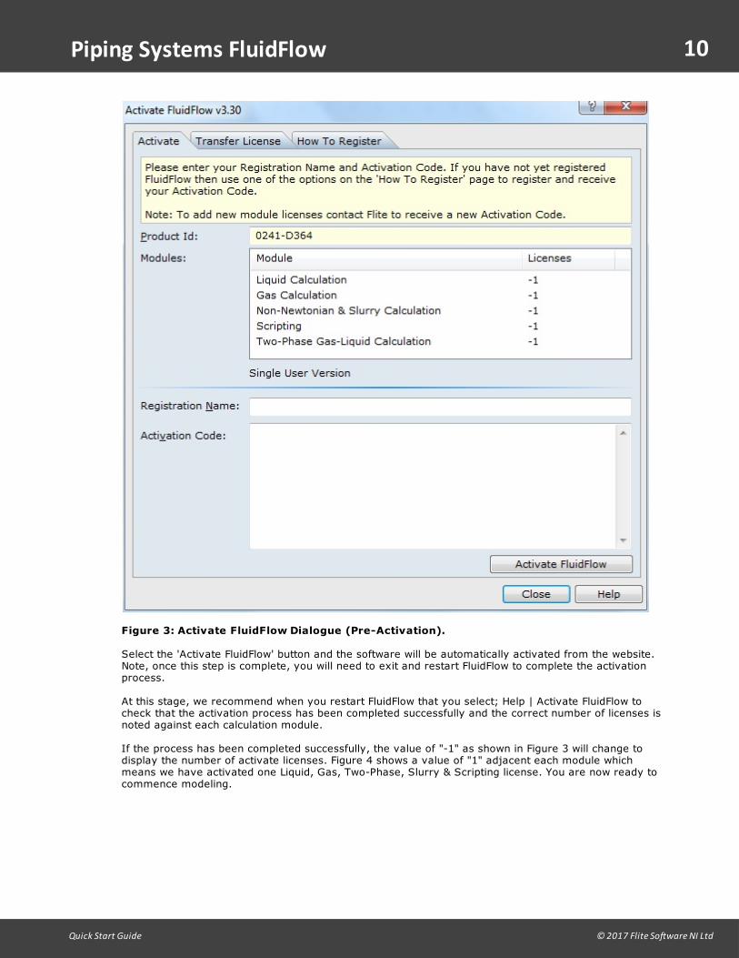
Figure 3: Activate FluidFlow Dialogue (Pre-Activation).

Select the 'Activate FluidFlow' button and the software will be automatically activated from the website.Note, once this step is complete, you will need to exit and restart FluidFlow to complete the activationprocess.

At this stage, we recommend when you restart FluidFlow that you select; Help | Activate FluidFlow tocheck that the activation process has been completed successfully and the correct number of licenses isnoted against each calculation module.

If the process has been completed successfully, the value of "-1" as shown in Figure 3 will change todisplay the number of activate licenses. Figure 4 shows a value of "1" adjacent each module whichmeans we have activated one Liquid, Gas, Two-Phase, Slurry & Scripting license. You are now ready tocommence modeling.

11



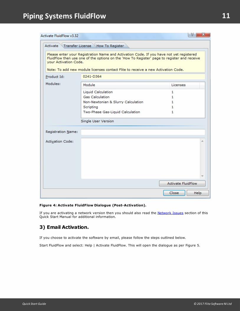
Figure 4: Activate FluidFlow Dialogue (Post-Activation).

If you are activating a network version then you should also read the Network Issues section of thisQuick Start Manual for additional information.

3) Email Activation.

If you choose to activate the software by email, please follow the steps outlined below.

Start FluidFlow and select: Help | Activate FluidFlow. This will open the dialogue as per Figure 5.

12



Figure 5: Activate FluidFlow Dialogue (Pre-Activation).

Email the Product ID to [email protected]. In the case of Figure 5, the Product ID is 0241-D364.The FluidFlow team will then reply with a Registration Name and Activation Code which you can useto activate the software.

Copy and paste the Registration Name and Activation Code into the relevant sections of the"Activate FluidFlow" dialogue box, taking care to ensure there are no spaces between characters of theactivation code. Now you can select the "Activate FluidFlow" button and then close the dialogue box.

Note, you will need to exit and restart FluidFlow to complete the activation process.

At this stage, we recommend when you restart FluidFlow that you select; Help | Activate FluidFlow tocheck that the activation process has been completed successfully and the correct number of licenses isnoted against each calculation module.

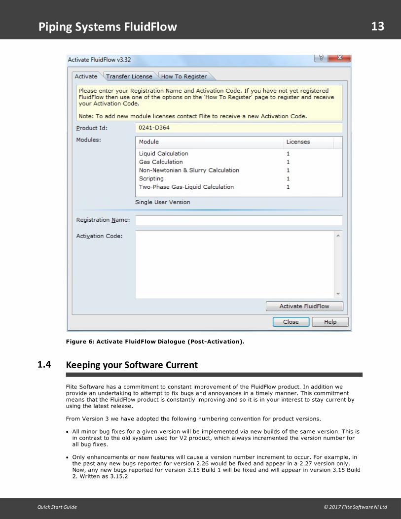
If the process has been completed successfully, the value of "-1" as shown in Figure 5 will change todisplay the number of activate licenses. Figure 6 shows a value of "1" adjacent each module whichmeans we have activated one Liquid, Gas, Two-Phase, Slurry & Scripting license. You are now ready tocommence modeling.


13



Figure 6: Activate FluidFlow Dialogue (Post-Activation).

1.4 Keeping your Software Current

Flite Software has a commitment to constant improvement of the FluidFlow product. In addition weprovide an undertaking to attempt to fix bugs and annoyances in a timely manner. This commitmentmeans that the FluidFlow product is constantly improving and so it is in your interest to stay current byusing the latest release.

From Version 3 we have adopted the following numbering convention for product versions.

· All minor bug fixes for a given version will be implemented via new builds of the same version. This isin contrast to the old system used for V2 product, which always incremented the version number forall bug fixes.

· Only enhancements or new features will cause a version number increment to occur. For example, inthe past any new bugs reported for version 2.26 would be fixed and appear in a 2.27 version only.Now, any new bugs reported for version 3.15 Build 1 will be fixed and will appear in version 3.15 Build2. Written as 3.15.2

14



· All version numbers have the format [Major Version].[Minor Version] Build Number, for example, 3.22Build 5 means a Version 3 product with a Minor Version number of 22 and a Build Number of 5. Writtenas 3.22.5

It is your responsibility to keep your software current via our website. We have a Software AssurancePolicy that enables continued access to the downloads area of our website:


1.5 Network Issues

Note: This section is only relevant if you have the Network module.

Installation Instructions

· Download FF3SETUP.EXE and either physically at your server or connecting via Remote Desktop

Connection (or similar software), Run the application.

· When installing FluidFlow3 on your network server, select Yes when prompted “Are you

installing on a NETWORK server?” . This will create a PSFF.INI (text) file, with a NetworkAccessFolderentry that points to the location of the license file on your server.

Refer to NOTE 1 below for information about configuring your FluidFlow3 network installation.

Activate FluidFlow3 on your network server to create the license file in the folder pointed to be PSFF.INI |NetworkAccessFolder. Note: You will need to do this either physically directly at the server machine, orvia Terminal Services/RDC.

Activation Instructions

· Start the FluidFlow3 License Manager (FluidFlow3LM.EXE) located in the same folder as PSFF.EXE

on your server.

· Go to the ‘Activate’ page.

· Enter:

Username: ******

Password: ******

· Click the 'Activate FluidFlow3' button.

Refer to NOTE 2 below for information about activating your FluidFlow3 network installation.

· Start FluidFlow3 on your server – username: Administrator; password: psff

· Select the ‘Database | Configure Users…’ menu item and add your FluidFlow3 users.

· Provide your users with a link to PSFF.EXE on your server.

http://www.fluidflowinfo.com/Downloads/Downloads.asp

15



NOTE 1: Configuring your Network Installation (Sharing Folders andSetting Permissions).

When you install FluidFlow3 the setup program creates a configuration text file - PSFF.INI - in the samefolder as the application (PSFF.EXE), typically C:\Program Files (x86)\Flite\FluidFlow3.

This file will contain three entries: the location of the equipment data (DataFolder); the location of theuser preferences (PreferencesFolder), and the location of the license file (NetworkAccessFolder). Theseare the only folders in FluidFlow3 that users *need* to have read-write access to for the application tofunction correctly. The FluidFlow3 application folder (and subfolders) require only read access.

FYI: The DataFolder needs to be read-write so that you can edit Line Equipment items such as valvesand Pumps via the ‘Databases’ menu item. The PreferencesFolder is where FluidFlow3 stores user-specific settings, e.g., ‘Options | Calculation’. The NetworkAccessFolder is where the application trackswho is logged on against what is valid for their license.

The PSFF.INI entries default to folders under “[Public Documents]\Flite”. The “Public Documents” folder istypically C:\Users\Public\Documents – you can determine where it is on your machine by putting %PUBLIC% into the Address Bar of Windows Explorer.

When you do a network installation – by answering Yes to the “Are you installing on a NETWORKserver?” prompt - your PSFF.INI will look like (with YourServer replaced by the name of your serverm/c):

[Options]DataFolder=\\YourServer\C$\Users\Public\Documents\Flite\FluidFlow3\DataPreferencesFolder=\\YourServer\C$\Users\Public\Documents\Flite\FluidFlow3\PreferencesNetworkAccessFolder=\\YourServer\C$\Users\Public\Documents\Flite\FluidFlow3

This is where an issue might arise as FluidFlow3 assumes the C drive will be shared when you do anetwork installation. We would recommend that you do *not* share the C drive itself, but share the“[Public Documents]\Flite\FluidFlow3” folder instead.

To do this: right-mouse click the FluidFlow3 folder name in Windows Explorer. Select ‘Properties |Sharing | Advanced Sharing’ and check the ‘Share this folder’ option:

16



C lick the ‘Permissions’ button and give full control to the ‘Everyone’ group:

17



If you share the FluidFlow3 folder (as described above), you need to modify PSFF.INI to reflect that. Forexample:

[Options]DataFolder=\\YourServer\FluidFlow3\DataPreferencesFolder=\\YourServer\FluidFlow3\PreferencesNetworkAccessFolder=\\YourServer\FluidFlow3

NOTE 2: Activating FluidFlow3

There are a few ways to activate FluidFlow3, however, for a Network license activation, you *do* needto have access to the server machine (either physically, or via Terminal Server/Remote DesktopConnection/similar software.) This access is required to be able to get the correct Product Id (i.e., theHard Disk Serial No.) for the server, or to run the FluidFlow3 License Manager.

Activating FluidFlow3 (via Activation Code):

· Start FluidFlow3 on the server machine (either physically or remotely logging in.)

· Select the ‘Help | Activate FluidFlow…’ menu item and make a note of the Product Id.

· Send this Product Id to [email protected] (or your local distributor) and an Activation Code

will be generated and emailed back to you.


18



· In the ‘Activate FluidFlow’ dialog, paste the code into the ‘Activation Code’ input area, along with

the ‘Registration Name’ provided.

· Restart FluidFlow3.

NOTE: You can generate the Activation Code yourself by logging into the your account on our server:

· Start FluidFlow3 on the server machine and get the Product Id from the ‘Help | Activate

FluidFlow…’ menu item.

· Log in to your account on our server (http://www.fluidflowinfo.com/portal/login.php). Please

contact [email protected] (or your local distributor) for your Username and Password, if you donot have them.

· Select ‘Generate Code’ from the ‘Your Info’ drop-down.

· Ensure the correct Product Id is entered.

· Click the ‘Generate Activation Code’ button.

· Copy and paste the generated code into the ‘Activate FluidFlow’ dialog in FluidFlow3 and restart

the application.

Activating FluidFlow3 (via License File, FF3.LIC):

· Start FluidFlow3 on the server machine (either physically or remotely logging in.)

· Select the ‘Help | Activate FluidFlow…’ menu item and make a note of the Product Id.

· Send this Product Id to [email protected] and a License File (FF3.LIC) will be created and

emailed back to you.

· Stop FluidFlow3.

· Copy the FF3.LIC License file to the NetworkAccessFolder on the server.

· Restart FluidFlow3.

NOTE: The “NetworkAccessFolder” is where the FF3.LIC License file should be located. The location ofthis folder will vary depending on the version of FluidFlow3 on your installation, or if you are using aPSFF.INI:

· If a PSFF.INI has been created in the application folder (by default, C:\Program Files (x86)

\Flite\FluidFlow3), the NetworkAccessFolder entry should hold the location of where FF3.LIC should beplaced.

· If using FluidFlow v3.31 or lower, and there is no PSFF.INI/NetworkAccessFolder entry, the

FF3.LIC file should be placed in the application folder, typically, C:\Program Files (x86)\Flite\FluidFlow3.

· If using FluidFlow v3.32 or higher, and there is no PSFF.INI/NetworkAccessFolder entry, the

FF3.LIC file should be placed in the “[Public Documents]\Flite\FluidFlow3” folder, typically, C:\Users\Public\Documents\Flite\FluidFlow3. You can determine the “base” Public Documents folderby putting %PUBLIC% in the Windows Explorer address bar and searching from there.

http://www.fluidflowinfo.com/portal/login.php



19



Activating FluidFlow3 (via the FluidFlow3 License Manager, FluidFlow3LM.EXE):

NOTE: Depending on the version of your existing installation, you may not have this application. It canbe downloaded from http://www.fluidflowinfo.com/ffdownloads/v3/FluidFlow3LM.zip. Unzip this to thesame folder as the FluidFlow3 application (PSFF.EXE) on your server.

· Ensure that FluidFlow3 is not running on the server machine.

· Start the FluidFlow3 License Manager (FluidFlow3LM.EXE) on the server machine (either

physically or remotely logging in.)

· Select the ‘Activate’ page, and enter your Username and Password. Please contact

[email protected] (or your local distributor) for your Username and Password, if you do not havethem.

· Click the ‘Activate FluidFlow3’ button.

Client Setup

After installing and activating FluidFlow on the network server you can set up the client machine byplacing a link on the client's desktop to FluidFlow. To do this, assuming that FluidFlow3 is the name of theshared folder:

1. Right-click on the desktop and select the 'New | Shortcut' menu item.

2. Type the location of the PSFF.EXE file, e.g., '\\Server\FluidFlow3\PSFF.exe' and click 'Next'.

3. Enter the title for the shortcut, e.g., 'FluidFlow3 (Network)' and click 'Finish'.

Note: If you do place a link on the desktop to FluidFlow on the network server, then this may affect thestartup speed of the client machine. This is because on startup the client will search the NetworkNeighbourhood to find the link's target. Normally, if the network server is always on, this will take nonoticeable time; however, if the network server is down, you may notice some small extra delay instartup. (Note: This is not specific to FluidFlow, but is true of all applications linked to a networkresource.)

Help Files on the Network

Security updates to Microsoft Windows have introduced some severe restrictions for accessing HTML Help(CHM) files across network drives. Under Windows most file links in HTML Help files will now generallynot work at all and HTML Help itself is also severely restricted. Without registry changes on the user'scomputer, HTML Help now cannot be used at all on networks. This has an effect on the FluidFlow3Network Version as all client machines that try to display the Help file will receive a "Page not found"message.

More details and a fix for this problem are available on the Help & Manual(http://www.helpandmanual.com/products_hhreg.html) website.

Alternatively, there is a workaround to allow a client machine to display Network-based HTML Help files,but it does involve modifying the Registry on the client machine. To do this:

1. Click 'Start', click 'Run', type 'regedit', and then click 'OK'.

2. Locate and then click the following subkey:

HKEY_LOCAL_MACHINE\SOFTWARE\Microsoft\HTMLHelp\1.x\ItssRestrictions

Note: If this registry subkey does not exist, create it. To do this, follow these steps:

a. On the 'Edit' menu, point to 'New', and then click 'Key'.

b. Type 'ItssRestrictions', and then press 'ENTER'.

http://www.fluidflowinfo.com/ffdownloads/v3/FluidFlow3LM.zip


20



4. Right-click the ItssRestrictions subkey, point to 'New', and then click 'DWORD Value'.

5. Type 'MaxAllowedZone', and then press 'ENTER'.

6. Right-click the MaxAllowedZone value, and then click 'Modify'.

7. In the Value data box, type '1', and then click 'OK'.

This will allow you to access CHM files on a shared network folder. For more information see:http://support.microsoft.com/?kbid=896054

Note: Always make a backup of the Registry before making any modifications so that you can 'rollback'the changes if anything goes awry. To do this, run Regedit, select the 'File | Export' menu item, selectthe 'All' option from 'Export Range', enter a filename and click 'Save'. You can later use the 'File |Import' menu item if you want to revert to your original Registry.

Help Files on the Network - Alternative Solution

FluidFlow3 also supports browser-based help. If you wish to use this please download the FF3BHELP.ZIPfile from our website - http://www.fluidflowinfo.com/ffdownloads/v3/FF3BHelp.zip - and unzip it to theFluidFlow3\Help folder to give \FluidFlow3\Help\FFEnglish and \FluidFlow3\Help\QuickStart folders.

For FluidFlow3 to use this, create PSFF.INI (if it does not already exist) in the same folder as PSFF.EXEand add an Options | UseBrowserHTMLHelp entry:

[Options]

UseBrowserHTMLHelp=1

Troubleshooting

The most usual issues reported for network installations and their resolutions are given below...

1. Unable to ActivateThis is because you are trying to activate from a client machine. This is not possible because

you are running the application in the client workspace and not the server workspace. For the purpose ofactivation ONLY, you can overcome this issue by connecting to the server via remote desktop (terminalservices, citrix etc) or being physically present at the server to activate. So to activate a networkversion, run the application via remote desktop, or be physically at the server.

Another possible reason for "unable to activate" is because you do not have the correctread/write/modify permissions to the folder (and all sub folders) where FluidFlow is installed.

2. "User Limit [1] reached. No more users allowed." message always displayed no matter how manylicenses. This is caused by the incorrect sharing of the FluidFlow folder. For more information see theNetwork Installation section above.

21



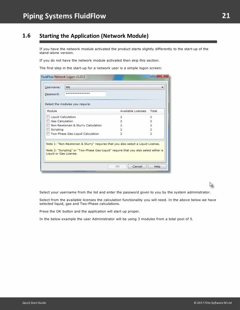
1.6 Starting the Application (Network Module)

If you have the network module activated the product starts slightly differently to the start-up of thestand-alone version.

If you do not have the network module activated then skip this section.

The first step in the start-up for a network user is a simple logon screen:

Select your username from the list and enter the password given to you by the system administrator.

Select from the available licenses the calculation functionality you will need. In the above below we haveselected liquid, gas and Two-Phase calculations.

Press the OK button and the application will start up proper.

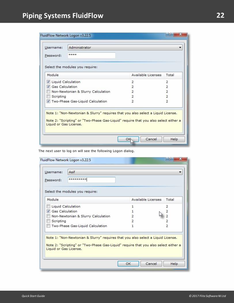
In the below example the user Administrator will be using 3 modules from a total pool of 5.

22



The next user to log on will see the following Logon dialog.

23



Notice that there are now less licence's available as liquid, gas and Two-Phase modules were taken byAdministrator who logged on first.

You can skip to the next section unless you are the administrator and wish to set up a group of users,delete a user, or change a password.

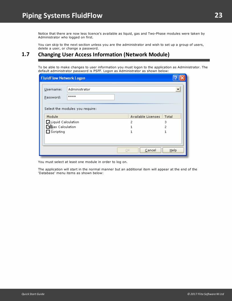
1.7 Changing User Access Information (Network Module)

To be able to make changes to user information you must logon to the application as Administrator. Thedefault administrator password is PSFF. Logon as Administrator as shown below:

You must select at least one module in order to log on.

The application will start in the normal manner but an additional item will appear at the end of the'Database' menu items as shown below:

24



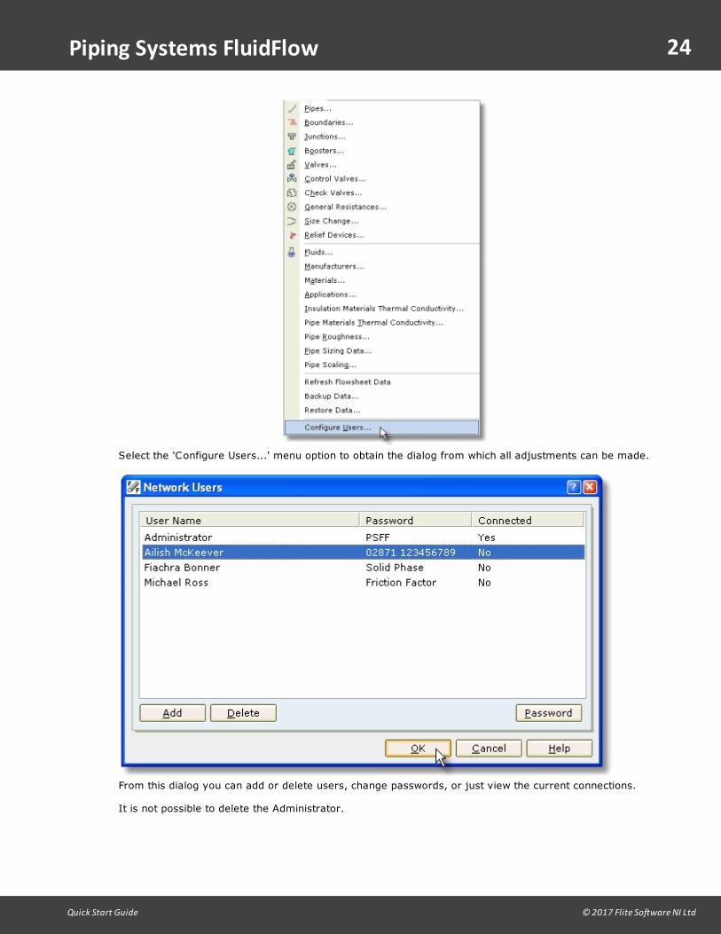
Select the 'Configure Users...' menu option to obtain the dialog from which all adjustments can be made.

From this dialog you can add or delete users, change passwords, or just view the current connections.

It is not possible to delete the Administrator.

25



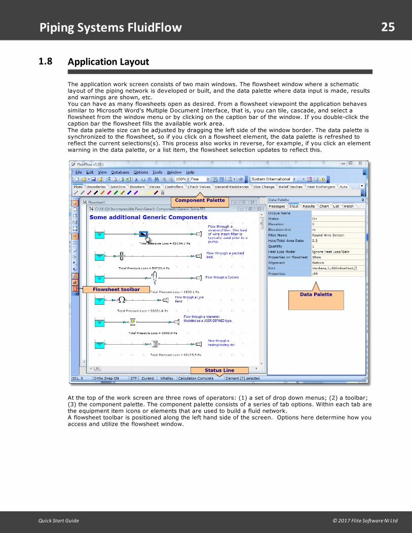
1.8 Application Layout

The application work screen consists of two main windows. The flowsheet window where a schematiclayout of the piping network is developed or built, and the data palette where data input is made, resultsand warnings are shown, etc.You can have as many flowsheets open as desired. From a flowsheet viewpoint the application behavessimilar to Microsoft Word's Multiple Document Interface, that is, you can tile, cascade, and select aflowsheet from the window menu or by clicking on the caption bar of the window. If you double-click thecaption bar the flowsheet fills the available work area. The data palette size can be adjusted by dragging the left side of the window border. The data palette issynchronized to the flowsheet, so if you click on a flowsheet element, the data palette is refreshed toreflect the current selections(s). This process also works in reverse, for example, if you click an elementwarning in the data palette, or a list item, the flowsheet selection updates to reflect this.

At the top of the work screen are three rows of operators: (1) a set of drop down menus; (2) a toolbar;(3) the component palette. The component palette consists of a series of tab options. Within each tab arethe equipment item icons or elements that are used to build a fluid network. A flowsheet toolbar is positioned along the left hand side of the screen. Options here determine how youaccess and utilize the flowsheet window.

26



1.9 Auto Equipment Sizing Example

FluidFlow includes a powerful auto-size feature which allows engineers to automatically size a range ofelements such as pipes, centrifugal pumps, fans, compressors, PD pumps, orifice plates, nozzles,pressure and flow control valves. Pressure relief valves and bursting disks can also be auto-sized to API& ISO standards for liquids, gases, steam and two-phase flow systems.

This example involves designing a cooling water distribution system to a bank of heat exchangers wherewe shall use orifice plates to balance the flow distribution. We shall also use the auto sizing functions todevelop the system design and size the pipes, pump and orifice plates.

Problem Statement:

It is desired to provide a balanced cooling water flow to four shell and tube heat exchangers HE1, HE2,HE3 and HE4. The size of the heat exchangers has already been determined from the processrequirement and is summarized in table 1.

Table 1

The cooling water is to flow through the heat exchangers and the design system inlet temperature will be15°C. The design temperature rise of the cooling water across each heat exchanger is 30°C. Theelevation of the all elements in this model is zero. The design duty pressure rise for this system is alsoknown, 2.5 bar.

Building the model in the FluidFlow flowsheet:

1. Place two known pressure boundary nodes on the flow sheet.2. Using the steel pipe element, connect the known pressure boundary nodes together as per Figure 1below. 3. Add the branch pipe connections, ensuring the branch at each tee junction is assigned correctly. 4. Insert the heat exchangers into each branch line.5. Insert thin orifice plates into the branch pipe connection serving each heat exchanger.

The basic model connectivity should appear as set out in Figure 1.

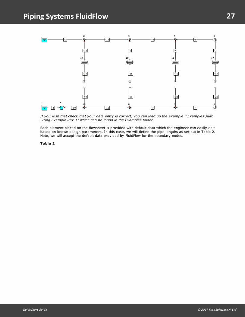
Figure 1

27



If you wish that check that your data entry is correct, you can load up the example "\Examples\AutoSizing Example Rev 1" which can be found in the Examples folder.

Each element placed on the flowsheet is provided with default data which the engineer can easily editbased on known design parameters. In this case, we will define the pipe lengths as set out in Table 2.Note, we will accept the default data provided by FluidFlow for the boundary nodes.

Table 2

28



Select all the heat exchangers at once by holding the SHIFT key and left mouse-clicking on each. All heatexchangers should now be highlighted on the flowsheet. From the Input tab of the Data Palette, set theHeat Loss Model to Fixed Transfer Rate, the heat transfer direction to Into the Network and the HeatTransfer Unit to kW. We have now set all common parameters for the heat exchangers in one step.

The next step is to define the heat load for each heat exchanger (see Table 1).

The design pump pressure rise is 2.5 bar. We can therefore set the centrifugal pump to AutomaticallySize from the Input Tab on the Data Palette. In doing so, we have two sizing options available; Size forFlow and Size For Pressure Rise. Select Size For Pressure Rise and defined the Design Pressure Changeas 2.5 bar. Using the data available for the heat exchangers, we can determine the design mass flow rate from theheat balance (Q = m x c x ∆T). The heat transferred to the cooling water will therefore be:

Heat Transferred (W) = mass flow (kg/s) x specific heat capacity (J/kg) x temperature rise (°C)

The specific heat of water at 30°C is approx 4154 J/kg, so from Table 1 we see that the mass flowneeded to HE1 will be 370000 / (4154 x 30) = 2.969 kg/s. Summarizing in Table 3.

Table 3

29



Since we can auto-size our components, we can define the design flow rate at each orifice plate bysetting the Automatically Size option on the Input tab of the Data Palette to On. We now have two sizingmodels to choose from, Size for Flow and Size for Pressure Loss. As we know the flow rate, select Sizefor Flow. The next step is to enter the mass flow rates noted in Table 3 for each orifice plate.

The Sizing Model for pipes is Economic Velocity by default. This means that FluidFlow will determine theExact Economic Size pipe diameter based on the calculated Economic Velocity. This velocity is a functionof the fluid physical properties, the pipe materials, various capital and installation costs and the operatinghours/year. This value is calculated from the Generaux equation and the calculation uses the values andconstants stored in the pipe sizing database. Economic velocity is changing (generally decreasing) withtime, particularly as energy costs have increased rapidly in recent times. Flite Software keeps thesevalues up to date, which is one of the many reasons you should keep your software current. Economicvelocity is meant to be a guide for pipe sizing it is NOT a strict criteria for sizing pipes. For example youwould not use this value to size pipes where two phase flow is present, or where plant operation isintermittent, or where materials can degrade at high velocities, or for Non-Newtonian flows.

We wish to develop an efficient system design and as such, we are going to retain the Economic Velocitysizing model.

We are now in a position to calculate the model. The solved system should appear as set out in Figure 2.

Figure 2

The flow distribution has been shown and if we view the results for any of the four heat exchangers, wecan see that the inlet temperature is 15°C and the outlet temperature is 45°C (based on our design 30°Ctemperature rise).

Note, we also have three warning messages indicating high velocities in the pipelines highlighted in RED.

If you wish that check that your data entry is correct, you can load up the example "\Examples\AutoSizing Example Rev 2" which can be found in the Examples folder.

30



A quick check on the results for each of the pipes with a high velocity warning indicates velocities in therange of 4.5 m/s which is considered high. We therefore need to review the pipe diameter. The diameterof each of these pipes is the default value of 2 inch which is 52.5mm. FluidFlow has determined aneconomic pipe size of approx. 101mm for each of these three pipes. We therefore need to select thenext closest standard size match. Lets try a 4 inch schedule 40 pipe.

You can multi-select the three pipes by holding the SHIFT key and left mouse-clicking on each pipe. Fromthe Input tab on the Data Palette, access the pipes database and change the pipe to 4 inch schedule 40pipe. Press Calculate to refresh the results for the system.

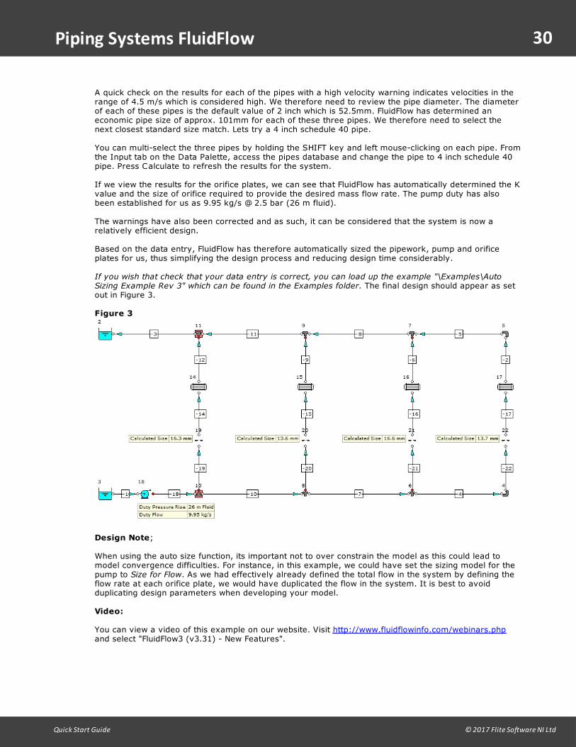
If we view the results for the orifice plates, we can see that FluidFlow has automatically determined the Kvalue and the size of orifice required to provide the desired mass flow rate. The pump duty has alsobeen established for us as 9.95 kg/s @ 2.5 bar (26 m fluid).

The warnings have also been corrected and as such, it can be considered that the system is now arelatively efficient design.

Based on the data entry, FluidFlow has therefore automatically sized the pipework, pump and orificeplates for us, thus simplifying the design process and reducing design time considerably.

If you wish that check that your data entry is correct, you can load up the example "\Examples\AutoSizing Example Rev 3" which can be found in the Examples folder. The final design should appear as setout in Figure 3.

Figure 3

Design Note;

When using the auto size function, its important not to over constrain the model as this could lead tomodel convergence difficulties. For instance, in this example, we could have set the sizing model for thepump to Size for Flow. As we had effectively already defined the total flow in the system by defining theflow rate at each orifice plate, we would have duplicated the flow in the system. It is best to avoidduplicating design parameters when developing your model.

Video:

You can view a video of this example on our website. Visit http://www.fluidflowinfo.com/webinars.phpand select "FluidFlow3 (v3.31) - New Features".

http://www.fluidflowinfo.com/webinars.php

31



1.10 Design of a Cooling Water System - Part 1

This example will work through the design development of a cooling water distribution system. In doingso, this exercise will demonstrate some of the unique features of the software including the powerful auto-sizing functionality.

The topics covered in this example design are:

Ø Flowsheet and model building basics.

Ø How to enter data.

Ø How to interpret results.

Ø How to automatically size pipes and components.

Note, FluidFlow allows engineers to auto-size pipes, pumps, orifice plates, control valves and a range ofother fittings which simplifies the design process and reduces project design-time considerably.

Outline Project Brief:

It is desired to provide a balanced distribution of cooling water from a cooling tower to serve a total ofthree shell and tube heat exchangers HE1, HE2 and HE3. The size of the heat exchangers has alreadybeen determined from the process requirement and is summarized in Table 1.

Table 1

Design Criteria:

Ø The cooling water is to flow through the tubes of each exchanger and the maximum inlet summertemperature of the cooling water will be 25°C.

Ø The design temperature rise of the cooling water across each each heat exchanger is 10°C.

Ø The elevation of the exchangers above the pump centerline is 3 m and the exchangers areapproximately 8 M apart.

Ø Each exchanger has 2 tube passes.

Ø The elevation of the cooling tower inlet above the pump centerline is 6m and the manufacturer of thecooling tower requires a minimum pressure loss of 30000 Pascals for the flow distribution to workeffectively.

As part of the design development, we need to design/specify the following items;

Ø Pipe sizes to be used.

Ø The method we will use to balance the flow through each exchanger.

Ø How to make a pump selection.

32



Ø We need to consider what happens to the exit cooling water temperature of HE2 if the heat load isincreased by 33%.

Building the model in the FluidFlow flowsheet:

With the design of all systems the initial question we need to answer is where do we start and end themodel, i.e. where do we and how do we define the model boundaries. For this design we will start themodel at the cooling tower sump and end the model at the top of the cooling tower. This means theactual cooling tower will not be included in this model. Most cooling water systems have a supply headertaking fresh cooling water to each individual exchanger and a collection return header. We will thereforeuse this same approach.

Finally, before we start building the model we need to consider the cooling water flow rate we need toeach exchanger branch. The flow to each exchanger is determined by a heat balance equation;

Heat Transferred (W) = Mass flow (kg/s) x Specific Heat Capacity (J/kg) x TemperatureRise (°C).

or simply

Q = m x c x ∆T.

The specific heat of water at 30° C is approximately 4154 J/kg, so from Table 1 we see that the massflow needed to HE1 will be 200000 / (4154 x 10) = 4.81 kg/s. The required mass flow rate of water toeach exchanger is summarized in Table 2 below.

Table 2

We will now start building the model by placing three shell and tube exchangers onto the flowsheet.Select the shell and tube exchanger icon by clicking on the Heat Exchangers Tab on the ComponentPalette.

Place three shell and tube heat exchangers onto a new flowsheet as shown below:

33



As we drop each element (or component) onto the flowsheet, default data is associated with the element.The default data for each element can be seen in the Data Palette by clicking on the Input Tab. Often weneed to change some value(s) in the default data to meet our needs. For now we will continue buildingand come back later to change each individual element as necessary.

The reason we are deferring this task is that there are many group features built into FluidFlow to aiddata editing and setup, which we can use feature later.

Next we will add the two boundaries.

Inlet Boundary:

For the cooling water inlet boundary we need a boundary that can represent the cooling water sump. Weknow that the sump is open to atmosphere and that during normal operation the liquid level in the sumpis 0.5m above the pump centerline.

If we specify the pressure at any boundary then FluidFlow will calculate the flow that will be delivered tothe system. In our design we know the design flow that is needed, because this is determined by theheat load of the exchangers. Later we will make a pump selection that will provide us with the correctflow and design duty pressure rise across the system.

Select the Known Pressure boundary icon by clicking on the Boundaries Tab on the Component Palette.Place the Known Pressure element on the flowsheet anywhere below the three heat exchangers.

Outlet Boundary:

The collection return line eventually leads back to a cooling tower. At this boundary we know thepressure that we must have above in order for the system to work as the cooling tower manufacturerrequires a minimum pressure loss of 30000 Pascals. The water pressure necessary at the exit boundaryis the sum of the elevation we need to rise to the top of the cooling tower + any pressure required toovercome the loss in the flow distribution system feeding the cooling water tower. The elevation of thecooling tower inlet above the pump centerline is 6m. We will therefore select a Known Pressure elementfor the exit boundary.

At this point the flowsheet should look something like;

34



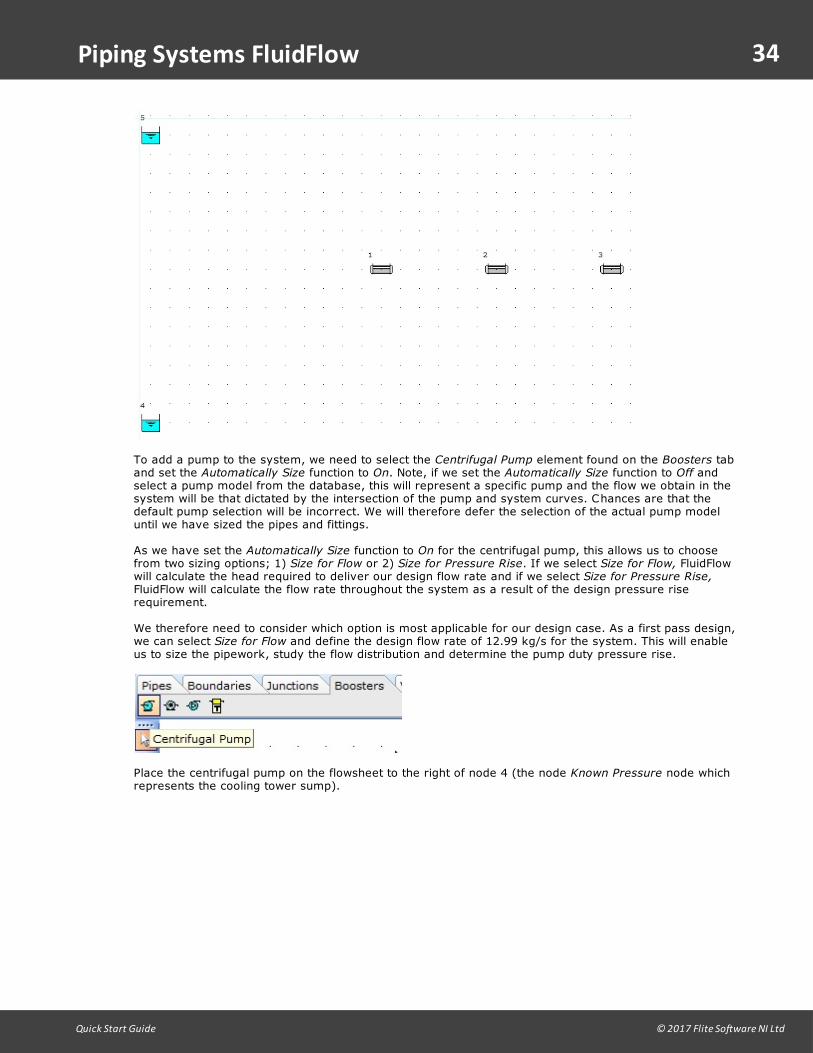
To add a pump to the system, we need to select the Centrifugal Pump element found on the Boosters taband set the Automatically Size function to On. Note, if we set the Automatically Size function to Off andselect a pump model from the database, this will represent a specific pump and the flow we obtain in thesystem will be that dictated by the intersection of the pump and system curves. Chances are that thedefault pump selection will be incorrect. We will therefore defer the selection of the actual pump modeluntil we have sized the pipes and fittings.

As we have set the Automatically Size function to On for the centrifugal pump, this allows us to choosefrom two sizing options; 1) Size for Flow or 2) Size for Pressure Rise. If we select Size for Flow, FluidFlowwill calculate the head required to deliver our design flow rate and if we select Size for Pressure Rise,FluidFlow will calculate the flow rate throughout the system as a result of the design pressure riserequirement.

We therefore need to consider which option is most applicable for our design case. As a first pass design,we can select Size for Flow and define the design flow rate of 12.99 kg/s for the system. This will enableus to size the pipework, study the flow distribution and determine the pump duty pressure rise.

Place the centrifugal pump on the flowsheet to the right of node 4 (the node Known Pressure node whichrepresents the cooling tower sump).

35



We are now ready to start connecting pipes. FluidFlow makes pipe connecting very easy, because thereis no need to include bends. These are added for you as you draw the pipes. We will again defer the taskof editing data values as we connect pipes. Right now we are only concerned with building the modelconnectivity.

Click the Steel Pipe icon on the Pipes tab of the Component Palette.

As you move the cursor over the flowsheet the shape changes to a pipe icon . Click on theknown pressure boundary and then move the mouse to be directly over the pump element, then clickthe left mouse button.

FluidFlow will then complete the pipe connection from the cooling water sump to the pump. While thecursor is over the pump make a second left mouse click and then move the mouse cursor to the rightbeneath heat exchanger 3 and make another left mouse click. A pipe is created starting at the pump andterminating at an open end. Click on the open end and the position the cursor directly over the heatexchanger as shown below.

36



Click on the exchanger, to complete the connection from the open end to the far right heat exchanger.Notice that the open pipe will change to a bend automatically.

If you make a mistake, click on the selector icon, in the flowsheet toolbar, select the wrongly connectedelement and use the Ctrl + Delete keys together to delete the selected element. Alternatively, rightmouse-click and select "Delete" from the drop-down menu.

Selector Icon.

Your flowsheet should now appear as shown below.

Move the cursor over the pipe on the discharge side of the pump on the same grid position as heatexchanger 2. Notice how the cursor changes from a pipe to a split pipe as we move over a pipe that canbe split. If we click here the pipe will be split and we can make the connection to the middle heatexchanger.

The split pipe has converted itself into a Tee connection. This type of junction, because it is madedynamically, adjusts itself depending on the number of pipes connected. For example a single pipeconnected and the junction is an open ended pipe, two connected pipes and the junction transforms to abend, three connected pipes the junction becomes a tee or wye and with four connected pipes thejunction becomes a cross.

Make further connections so that we end up with a connected network as shown on the following image.

37



Turn on the pipe numbering from the flowsheet toolbar. Note that pipe numbers go from -1 ... -n andthat other elements (nodes and text) are numbered 1 ... n.

Changing the default data using the flowsheet and data palette:

Up until this point no data entry has been made, we have focused on describing the elementconnectivity. This means that each element will have default data values according to the currentenvironment set in use when the element was placed on the flowsheet (see Customizations andEnvironment section for more information about environment sets).

You can select any element on the flowsheet at any time by clicking on the element, after first using(clicking on) the selector icon. First we need to enter all the pipe lengths. Table 3 shows the pipe lengthsthat are fixed by the physical plant layout and also the number of bends in each pipe section.

Table 3

38



To enter the pipe lengths we can use one of two approaches. Either we can select pipes from theflowsheet or we can select pipes from the Lists Tab in the Data Palette. We will use the flowsheet in thisexample.

We can reduce the amount of data entry we make by recognizing the fact that some of the pipes areidentical. For example the main feed and return branches to each exchanger are identical (pipes -3, -5, -7, -8, -11 and -13). If we use the fact that we can make multiple selections on the flowsheet we canchange the length of all 6 pipes with one edit.

There are many ways to make multiple element selections, but for now we will use the mouse-clickmethod. To make multiple selections using mouse clicks on the flowsheet simply hold down the Shift keyand click each element you wish to select. If you make a mistake and select the wrong element just clickthe element again and it will deselect. Don't forget to keep the Shift key depressed as you are makingthe multiple selections. Use this method to select the six identical branch pipes. If you release the Shiftkey and click anywhere on the flowsheet other than on a selected element you will lose your selections.

39



To enter the pipe length of 3 m for each selected pipe, click on the Input tab in the Data Palette, move tothe Length row in the Input tab and change the length to 3.

Input Inspector Tab.

40



The length of all 6 pipes is changed in one edit. Change the length of the remaining pipes, (Hint: theheader and return sections -4, -6, -10 and -12 are identical).

Time to save our work. Use the File Save menu to save your work now. It is good practice to regularlysave your work.

To complete the pipe data entry we need to make 2 additional entries. For each pipe we need to specifya nominal size and we need to add further bends as shown in Table 3. We need to determine pipe sizeand FluidFlow can help us here, so we will defer this task and add the additional bends now.

There are 2 additional bends in each branch line, 3 in the supply line from the pump to the first branch(tee node 9) and 5 additional bends in the return line from the last return branch (tee node 12) to thecooling tower.

As we are dealing with an incompressible fluid, where the density change is small throughout thenetwork we can avoid entering all bends individually. Instead use the Quantity row for each bend we addin the Input Inspector to reduce the number of bends we need to add.

Design Note: This approach is NOT recommended where density changes throughout a pipe section aresignificant, i.e. compressible fluids.

Select the Junctions Tab in the component palette and click on the bend, then drop this bend into pipe. Ifyou need to create some additional length to pipe -1 on the flowsheet, click on the pump node (6), holddown the left mouse button and drag the node to a different location.

Add the remaining bends as shown highlighted in the flowsheet below.

Hold the Shift key and click on bends 14, 15, 16, 17, 18 & 19 and change the Quantity row in the InputInspector of the Data Palette from 1 to 2.

Click on bend 13 and change the quantity to 3. Click on bend 20 and change the quantity to 5. Thisalmost completes the data entry for the pipe data given in Table 3. All that remains for pipe entry is toset each pipe diameter.

41



You may have noticed that inserting an element in a pipe splits the pipe lengths into two equal segmentlengths. This is the default behavior but can be changed based on personal preferences if desired. Thiscan be achieved by selecting; Options | Environment | Component Defaults [F4].

Note, it is important to review all pipe lengths which have been affected as a results of insertingelements. In this case, we have set the length of the pipes in this system to reflect that shown in Table4.

Table 4

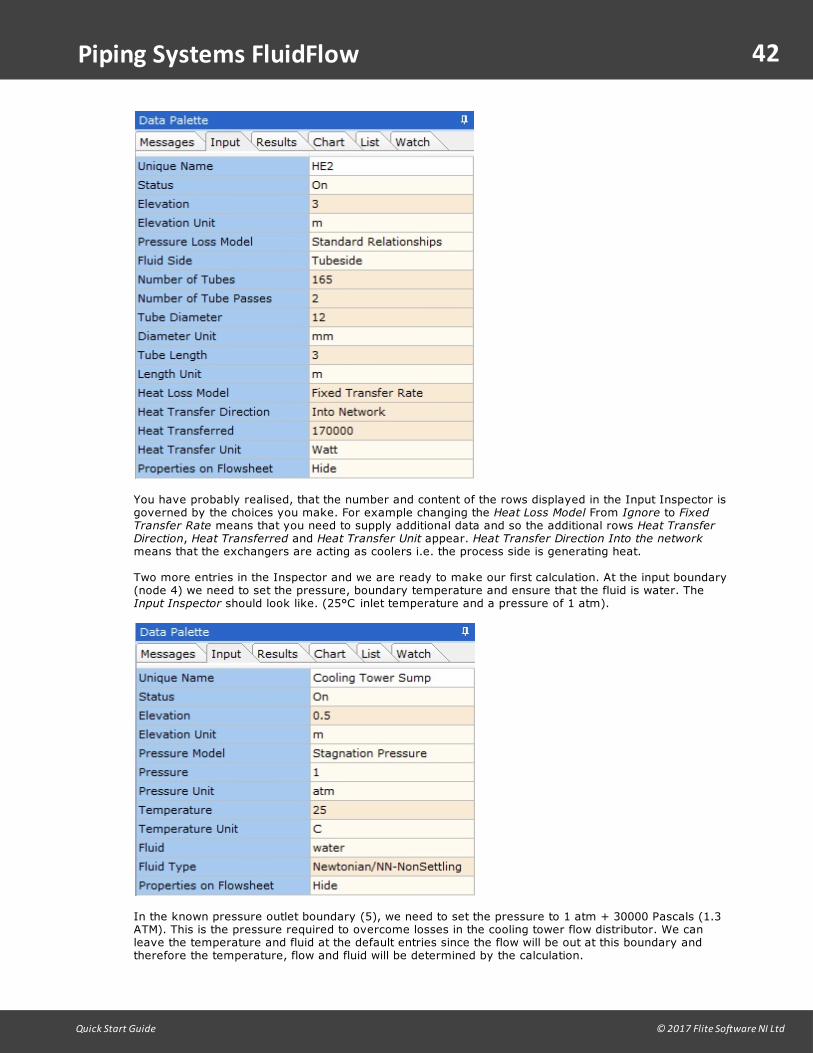
Click on each heat exchanger on the flowsheet and change the default data to reflect the tubeinformation provided in Table 1. The Input Inspector for HE2 is shown below.

42



You have probably realised, that the number and content of the rows displayed in the Input Inspector isgoverned by the choices you make. For example changing the Heat Loss Model From Ignore to FixedTransfer Rate means that you need to supply additional data and so the additional rows Heat TransferDirection, Heat Transferred and Heat Transfer Unit appear. Heat Transfer Direction Into the networkmeans that the exchangers are acting as coolers i.e. the process side is generating heat.

Two more entries in the Inspector and we are ready to make our first calculation. At the input boundary(node 4) we need to set the pressure, boundary temperature and ensure that the fluid is water. The Input Inspector should look like. (25°C inlet temperature and a pressure of 1 atm).

In the known pressure outlet boundary (5), we need to set the pressure to 1 atm + 30000 Pascals (1.3ATM). This is the pressure required to overcome losses in the cooling tower flow distributor. We canleave the temperature and fluid at the default entries since the flow will be out at this boundary andtherefore the temperature, flow and fluid will be determined by the calculation.

43



At the pump (node 6) we need to enter the design flow rate of 12.99 kg/s. The orientation of the pumpshould be set so that the red dot, which represents the pump discharge, points to pipe -2. If you need tochange this click on the Discharge Pipe (RED) row in the Input Editor.

Before we make the first calculation you should also check that elevations are correct for each element.In fluid flow calculations the relative elevations are important, which means that we need to select adatum or grade point. i.e. a point where all elevations are measured relative to. Normally we wouldselect the ground to represent a 0 elevation. In this example we will take the pump centreline asrepresenting 0 elevation. Check that your node elevations are;

Table 5

44



To complete the data input make sure that all pipe lengths are set to the values in Table 4. At this stagewe can leave the pipe diameters at the default values because our next task is to size all of the pipes.

Press the Calculate button. You should see FluidFlow quickly solve the network and flowdirectional arrows appear on the pipes in the flowsheet.

You can view the results in many ways. The simplest is to select the Results Tab in the Data Palette andclick on each heat exchanger in turn on the flowsheet. In the results table the only row we are interestedin at this stage is the mass flow through each exchanger. If we click on each exchanger in turn we cansee that the flows do not match what we need from a cooling viewpoint. This means that the coolingsystem is unbalanced and will not work as specified in the initial design definition. You should be able tosee that the flow through HE1 is greater than design and the flow through HE2 and HE3 is too low.

There is a useful way to view these results. Since we will be constantly referring to these flows we canshow them on the flowsheet. To do this click on the 3 exchangers, while holding down the shift key tomake a multi-selection then in the Input Inspector, change the Properties on Flowsheet row from Hide toShow, set the Alignment to Left and press the Properties button to obtain the following dialog.

45



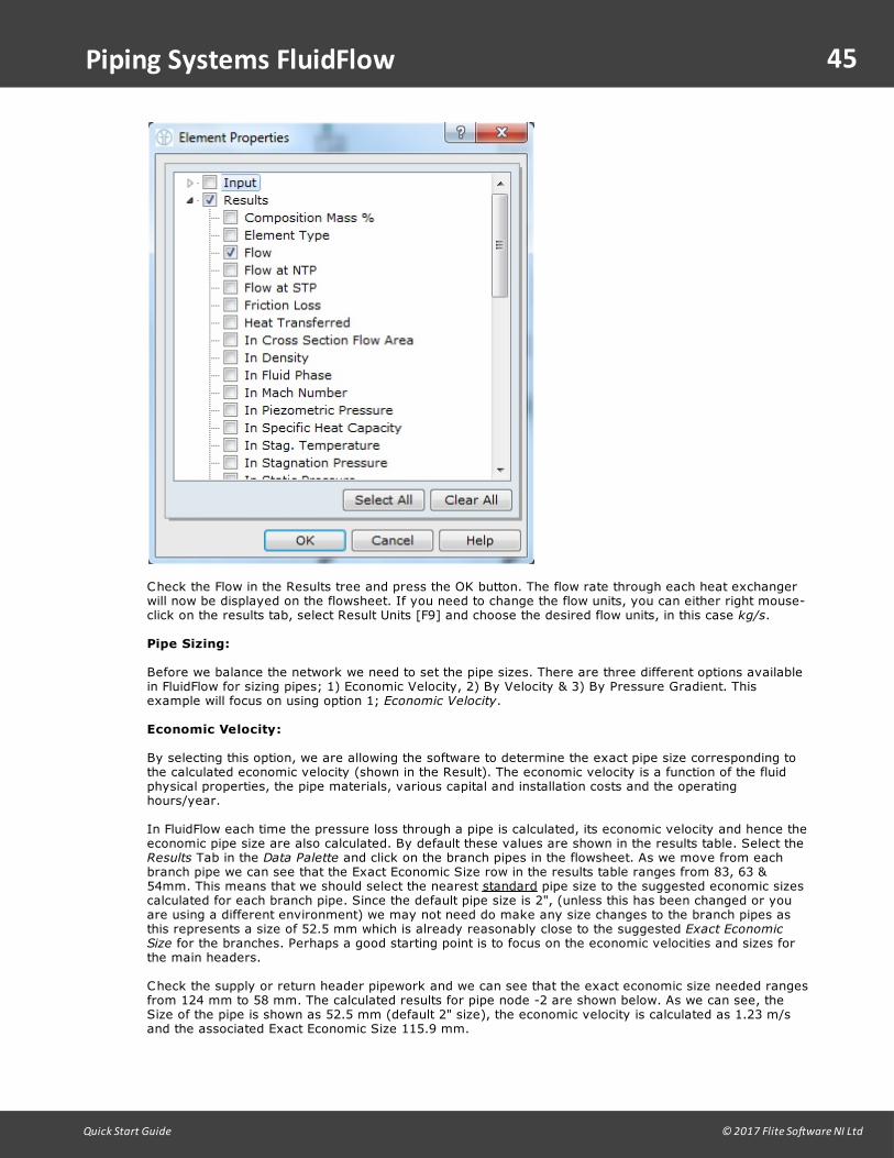
Check the Flow in the Results tree and press the OK button. The flow rate through each heat exchangerwill now be displayed on the flowsheet. If you need to change the flow units, you can either right mouse-click on the results tab, select Result Units [F9] and choose the desired flow units, in this case kg/s.

Pipe Sizing:

Before we balance the network we need to set the pipe sizes. There are three different options availablein FluidFlow for sizing pipes; 1) Economic Velocity, 2) By Velocity & 3) By Pressure Gradient. Thisexample will focus on using option 1; Economic Velocity.

Economic Velocity:

By selecting this option, we are allowing the software to determine the exact pipe size corresponding tothe calculated economic velocity (shown in the Result). The economic velocity is a function of the fluidphysical properties, the pipe materials, various capital and installation costs and the operatinghours/year.

In FluidFlow each time the pressure loss through a pipe is calculated, its economic velocity and hence theeconomic pipe size are also calculated. By default these values are shown in the results table. Select the Results Tab in the Data Palette and click on the branch pipes in the flowsheet. As we move from eachbranch pipe we can see that the Exact Economic Size row in the results table ranges from 83, 63 &54mm. This means that we should select the nearest standard pipe size to the suggested economic sizescalculated for each branch pipe. Since the default pipe size is 2", (unless this has been changed or youare using a different environment) we may not need do make any size changes to the branch pipes asthis represents a size of 52.5 mm which is already reasonably close to the suggested Exact EconomicSize for the branches. Perhaps a good starting point is to focus on the economic velocities and sizes forthe main headers.

Check the supply or return header pipework and we can see that the exact economic size needed rangesfrom 124 mm to 58 mm. The calculated results for pipe node -2 are shown below. As we can see, theSize of the pipe is shown as 52.5 mm (default 2" size), the economic velocity is calculated as 1.23 m/sand the associated Exact Economic Size 115.9 mm.

46



There is therefore a case for reducing the header size after each take off. This may reduce costs sincewe can utilise reducing Tee's.

We will use the economic size suggestions to change the pipe sizes in the following manner.

Set the pipe size in the supply header to the first branch (tee node 9) and in the return header from thelast branch (tee node 12) to be 4" Schedule 40 (Pipes -1, -2, -14, -21 and -9). Set the pipe in eachheader between the first and second branches to be 3" Schedule 40. At this stage, we will not makeadjustments to the rest of the header as it is already 2" by default which in some cases, is already nearthe suggested economic sizes. If we need to, we can re-visit this later if we still have high velocities inour lines.

Recalculate and save your work at this point. The model should now appear as shown below.

Note, you can rotate the junctions to enhance the presentation of the model by multi-selecting therelevant common nodes and selecting CNTRL + R (Edit | Rotate Node).

47



You may notice that you now have warning messages at four of the tee junctions. FluidFlow calculatescorrectly for reducing Tees, provided that you are using Idelchik, Miller or SAE types (this is the default).The tee's at nodes 9 and 12 have connecting pipe sizes 4, 3 and 2" and pressure conversion effects fromvelocity to static or vice versa are taken into account when calculating pressure losses at the tee. Clickon the tee, select the Input Tab and click the Nomenclature row in the Input Inspector if you need furtherinformation. For tees having 3 different branch sizes the loss relationships need to be extrapolated andyou may find that you have warning messages to this effect.

Warning messages are there to help you decide if you need to make design changes. In this case thewarning messages refer to the possible loss of calculation accuracy in the tee junctions becauserelationship data has been extrapolated. Since there are no other available pressure loss relationshipsavailable for these types of reducing tees we have no choice but to accept this warning. Still it isworthwhile checking on the calculated K values to ensure these are within an expected range (-2 to 10).You can also cross-check by using another loss relationship (say Miller type) and verify that thecalculated K values and pressure losses are similar. This is the case here and so we can safety ignorethe warnings. In fact we can turn off some of the less severe warnings, but this is not recommended.

Often, as engineers we like to keep header and return line sizes equal along the header and so a 4" oreven 3" header/return line size is also a valid solution. Remember to take into account all possibleoperating scenarios and future considerations before making your final design decisions. For example, ifwe knew there was a possibility of a 4th heat exchanger being added at some time in the future then itwould be a better solution to make the header and supply lines all 4". Pipe line sizing is always a balancebetween capital costs, operating costs and operating flexibility.

Pump suction lines should always be given careful consideration. We must always ensure that we havean entry head at the pump suction above the net positive suction head required by the pump + a safetymargin. FluidFlow will detect and warn if adverse conditions exist and as a first guess we will use 4"pipe.

Based on the changes made so far, the calculated results for the pump are as shown below.

48



Balancing the network:

We need to add additional elements in order to balance the network. In this design case, we are going toautomatically size orifice plates to achieve the required design flow rate of water in each branch. Usingorifice plates will allow you to drop pressure in a controlled manner in each branch so that the correctflow distribution is achieved. However, it is important to note that balancing is wasteful of energy andperhaps, an alternative design solution may be more applicable to your specific design case. In anyevent, using orifice plates will help us achieve our flow distribution goal.

To obtain the distribution required we will use 3 orifice plates, one in each branch. Using orifice plates isa cheap solution to the distribution issue. However it may not prove very flexible if process conditionsare likely to change. In this case using throttling valves may be a better solution.

Add the orifice plates as shown in the flowsheet below, set the Elevation of each orifice to be 3.75 m, setthe Automatically Size function to ON and set the Sizing Model to Size for Flow. We must now enter thedesign flow rate for each orifice plate as calculated in Table 2. By defining the flow rate at each orificeplate, we are by default entering the total mass flow rate for the system. In the first pass calculation, wehad already defined the total mass flow rate at the pump (12.99 kg/s). This will therefore lead toduplication in flow rates and as such, we need to change the pump Sizing Model to Size for PressureRise.

The design pressure rise from the pump can be established from adding the system pressure loss(calculated from pass 1 to be 117938.1 Pa) to the static head requirement which can be established fromthe equation P = r x g x H (P = 997 * 9.80665 * 6 = 58663 Pa). The design pressure rise thereforebecomes 176601.1 Pa. We can now enter this design value for the pump on the Input Inspector of theData Palette.

Recalculate the model to refresh the results. We can now see a different flow distribution.

49



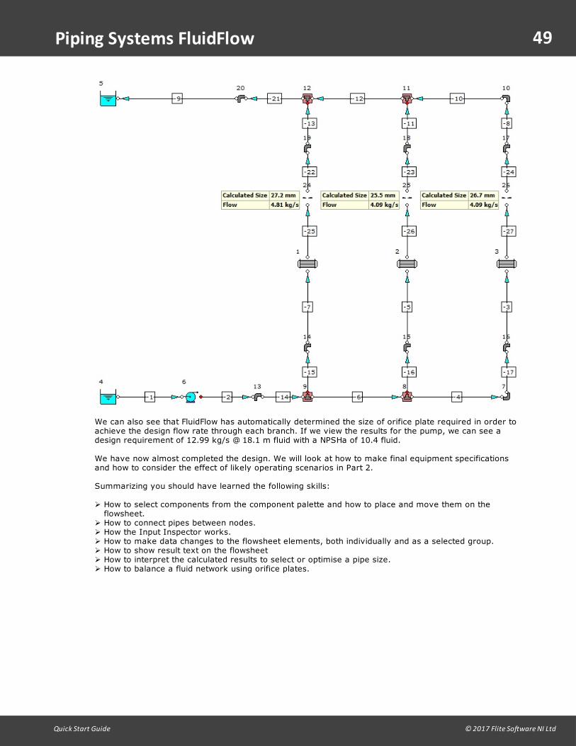
We can also see that FluidFlow has automatically determined the size of orifice plate required in order toachieve the design flow rate through each branch. If we view the results for the pump, we can see adesign requirement of 12.99 kg/s @ 18.1 m fluid with a NPSHa of 10.4 fluid.

We have now almost completed the design. We will look at how to make final equipment specificationsand how to consider the effect of likely operating scenarios in Part 2.

Summarizing you should have learned the following skills:

Ø How to select components from the component palette and how to place and move them on theflowsheet.

Ø How to connect pipes between nodes.Ø How the Input Inspector works.Ø How to make data changes to the flowsheet elements, both individually and as a selected group.Ø How to show result text on the flowsheetØ How to interpret the calculated results to select or optimise a pipe size.Ø How to balance a fluid network using orifice plates.

50



1.11 Design of a Tank Farm Gas Collection System

In this example we are not concerned with building the model and data entry. Instead we focus on theengineering.

Problem Statement:

It is desired to collect together the air vents from a group of 5 storage tanks holding a flammable,obnoxious liquid. The vent gas is to be treated in an activated carbon bed before finally passing toatmosphere.

In this problem we are only concerned with the situation that occurs as the tanks are filling. In ourscenario each tank, vents gas (for simplicity considered to be air), at the rate of which it can be filled.The exit gas vent from each yank is modeled as a known flow element, with the maximum tank fill ratesalready entered.

The remainder of the collection network has been built and can be opened from the \Examples folder"Non Sized Gas Collection System". Open the example and consider how we may answer the followingquestion.

1. Size all pipes so that the operating pressure under maximum filling rates does not exceed that allowedunder code API 650. This means no more than 1 psig operating pressure in each storage tank.

Considerations and approach:

We will take the worst case of all 5 tanks filling at one time.

To easily view the calculation result values we can use one of three possible techniques:

§ We can configure and turn on the fly by results. In this way we can move the mouse over theflowsheet and look at the result values we are interested in.

§ We can click the Results tab in the data palette on the left click on the flowsheet to select eachcomponent we are interested in.

§ We can show the results on the flowsheet.

It is important to state at the outset that there are many solutions to this problem. For example we couldincrease all line sizes until the pressure in each tank dropped below 1 psig. This would undoubtedly work,but as the lines are made of stainless steel and are of a reasonable length we may not wish to overdesign in this way due to cost considerations.

51



To start, let us consider the tank pressures if we use 2" pipe throughout (this is the case if we open theexample). You can see that each tank is over the maximum allowed pressure of 1 psig.

Click on any pipe and look at the results table in the data palette. You can see immediately that eachpipe is already larger than the size recommended according to the economic size. This is an importantpoint and illustrates that you cannot blindly set all pipe sizes to the suggested economic size in all cases.

Click on a few more components and consider the row titled "Non Recoverable Loss", this loss representsthe pressure loss that can never be recovered. It is this value that we must impact (reduce) if we are todesign a safe system.

You should quickly note that the majority of the system pressure loss occurs at over the packed bed.The packed bed represents a pressure loss of 0.6 psi out of a total of < 1psi available.

Using this knowledge, perhaps the best approach to take is increase the diameter of the bed to reducethe pressure loss, rather than increase the pipe size of each pipe. This now becomes a cost issue. Forexample is it less expensive to change the diameter of the bed, or use a different particle size in the bedrather than change the pipe sizes.

We do not have sufficient information to fully consider the available choices. What is important is thatyou recognise how to ustilise the power of FluidFlow to consider the alternative design scenarios.

If you have the scripting module you can automate this process.

An acceptable design changing only pipe sizes downstream of the Tee junction (node 15) is saved as"Pipe Sized Gas Collection System".

52



1.12 Design of a Cooling Water System - Part 2.

This is the concluding part to the design of a cooling water system, started in Part 1.

In this part we will select a specific manufacturer's pump to perform at the operating duty calculatedfrom the centrifugal pump element and consider the effect on the system if the heat load on exchanger 2(HE2) is increased by 33%.

Click on the centrifugal pump element on the flowsheet and the results tab on the data palette. If youare using the default "System International" environment you should see a result similar to;

OR

i.e. the design flow of 12.99 kg/s of water at 25° C needs a pressure rise of 176601 Pa in order tooperate at the design flows. We may wish to stop here and ask our preferred pump manufacturer tosuggest a pump to supply this duty. To do this we will need to convert the pump duty flow to a suitablevolumetric units and the calculated pressure rise needed to head units. You can use FluidFlow to do thisfor you automatically, however you may find it instructional to do the conversion now to m3/h and mFluid. The density of water, obtained from the results table is 997 kg/m3 and so the calculatedvolumetric flow will be 12.99 x 3600/997 = 46.9 m3/h. The head that the pump is required to producewill be 176601/(997 x 9.80665) = 18.1 m Fluid.

This information, together with the operating fluid and temperature conditions is enough for the pumpmanufacturer to make a selection and under normal circumstances this is all that is required.

It is better to allow the manufacturer to make the selection for the following reasons; pump selection isoften more than a simple hydraulic selection. Pump configuration, sealing and shaft load considerations,materials of construction etc are best handled by the manufacturer.

Even though the manufacturer is in a better position to make the selection it is still worthwhile and youcan often get a more flexible design by making some additional hydraulic considerations.

For the purpose of illustration we will use the inbuilt pump selector to make the selection at this dutypoint. From the menu select 'Tools | Equipment Performance Viewers | Pump Performance' to create thedialog shown below.

53



To use this tool change the Design Flow to be 46.9 m3/h, and as you click on each pump in the list theperformance data (Head, Efficiency, Best Efficiency and NPSH required) are shown for the currentlyhighlighted pump.

This means that you can move through each pump in the database and view how it will perform in thissystem. The pump shown above would be a suitable selection from NPSH and efficiency viewpoint, but isunsuitable because the head developed is greater that that required by our duty (18.1 m fluid).

Viewing the pump database provides a number of pumps that will fulfill the hydraulic and system needs.You may wish to consider some of the following models:

Girdelstone 32ns.DNP85-165.FA 253-4402Z.NM3196 2x3-10.

The best choice is the to select a pump operating near the best efficiency or a pump with the highestefficiency at the duty point.

To complete the example we will select the Gould pump NM 3196 2x3-10 MTX. The operatingperformance of this pump based on a design flow rate of 46.9 m3/h is as shown below.

54



To assign this pump to the model, click on the centrifugal pump node (6) and set "Automatically Size" to"Off". Change the pump model from the default pump, by clicking on the button in the Pump Model rowin the Input Editor and select the Gould NM 3196 2x3-10 MTX.

55



Notice that the pressure developed by this pump is higher than that needed and that the orifice size oneach branch has changed slightly in order to maintain the design flow rates specified.

56



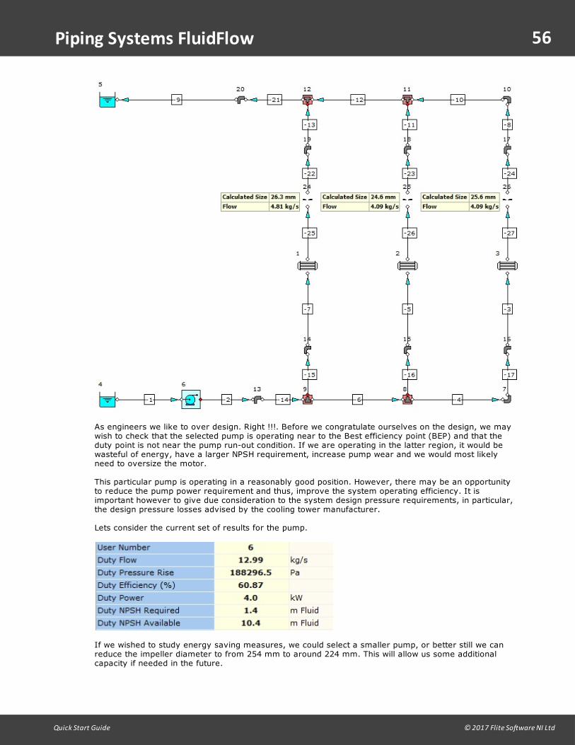
As engineers we like to over design. Right !!!. Before we congratulate ourselves on the design, we maywish to check that the selected pump is operating near to the Best efficiency point (BEP) and that theduty point is not near the pump run-out condition. If we are operating in the latter region, it would bewasteful of energy, have a larger NPSH requirement, increase pump wear and we would most likelyneed to oversize the motor.

This particular pump is operating in a reasonably good position. However, there may be an opportunityto reduce the pump power requirement and thus, improve the system operating efficiency. It isimportant however to give due consideration to the system design pressure requirements, in particular,the design pressure losses advised by the cooling tower manufacturer.

Lets consider the current set of results for the pump.

If we wished to study energy saving measures, we could select a smaller pump, or better still we canreduce the impeller diameter to from 254 mm to around 224 mm. This will allow us some additionalcapacity if needed in the future.

57



Lets apply this change to the impeller diameter from the Input tab. of the Data Palette. When werecalculate the model, we can see that the affinity laws have been applied and the power requirementhas reduced from 4.03 to 2.97 kW. We will also note however that the duty pressure rise has alsoreduced from 188296.5 to 133284.2 Pa. You may therefore wish to review this operating condition withthe cooling tower manufacturer. Details of the results of this simulation are shown below.

Note, by reducing the pump impeller diameter, the the pressure drop across the system reduces and theorifice plate diameters increase to maintain the desired flow rate which is reflected in the updatedflowsheet as shown below.

WARNING:

You should note that reducing the impeller diameter or changing the speed will produce a flexible design,but in this example, you can see from the adjusted pump chart that we are still operating away from thebest efficiency point and so this may not be the best solution.

58



Finally we need to consider increasing the heat load to HE2 by 33%. Change the heat transferred to be226,100 Watt, then recalculate. The temperature at the exit of the heat exchanger rises from 34.9°C to38.2°C. The temperature to the cooling tower increases from 34.9 to 36 °C. This increase in temperature is considered to be acceptable and we do not need to rebalance thesystem.

59



1.13 Configuration and Environment

Nearly all aspects of the FluidFlow application can be configured and customized. The configurationsettings that you change are saved, so that each time the application starts your own preferences areapplied. Some of the configurations will be familiar, such as changing the position of tool bars, addingbuttons, etc., because these customizations are commonly found in professional software.

Some aspects of the environment are stored as a subset called an Environment Set. You can make asmany environment sets as you need and change between them interactively.

An environment set is closely associated with the default input data and units for every component (fluidequipment item) that is available from the component palette as well as how and what calculation resultsyou wish to see.

Each environment set stores the following information, and can be easily accessed via a function key:

§ F4 - Provides access to the default settings for each component available from within the program.§ F5 - Provides access to the data columns you wish to export to Excel.§ F6 - Allows you to set up Fly By Options. A 'fly by' is the window that appears as you move the mouse

over a component on the active flowsheet. It is possible to set the fly by content for each component.§ F7 - Provides access to the columns you wish to print in your report, or export to Word, HTML, or PDF.§ F8 - Allows you to configure the contents of the table shown on the Results tab of the data palette.§ F9 - Allows you to individually set the calculated result units and the number of decimal places you

wish to use.

After a new installation of FluidFlow there are 2 environment sets already made for you. "SystemInternational" and "US Basic". These should form the basis of changes you make. Rather than makingthe changes to any of the basic sets provided, it is a better idea to make a renamed copy and make thechanges to the copy.

As an example of how to do this. First change environment to that you wish to copy from, you can dothis from the combo box on the main application toolbar.

Then select from the menu 'Configuration | Environment | Save Environment' to a new name.

60



Use the combo box in the main toolbar to change to the newly created environment and then customizeby say pressing F9 to change the result units in this set.

61



Here we have made the following changes from the original copy, we are displaying flow in l/min insteadof kg/s and we are displaying both pressure and pressure drop in bar a and bar. The number of decimalplaces shown has also been increased to reflect this change.

Load up an example such as "QA Incompressible Flow\Boosters\4 Pumps in Parallel 3 Operating" whichhas text on the flowsheet. Move to the Results tab on the data palette and then change environment set.You will see that the flowsheet results and the table results update immediately to show the newconditions.

1.14 Databases

A powerful feature of FluidFlow are the many associated databases that support and enhance theapplication. These include a database of fluid properties, databases that describe the performance andlimits of fluid equipment items, materials databases that hold pipe sizing and pipe insulation information,and a database of manufacturers, costs, and user-defined areas of application.

1.15 Fluids Database

The fluids database contains comprehensive thermo physical data for over 850 fluids. Thermo physicalproperties (density, viscosity, thermal conductivity, specific heat, physical constants and critical values,heat of vaporization, vapor pressure, and surface tension) are stored so that FluidFlow can completepressure loss calculations including heat transfer and phase change. The database is much more than a table of physical properties. Many "state of the art" physical propertyprediction methods are available, often used together with modern Equations of State such as Benedict

62



Webb Rubin, Lee Kesler, and Peng Robinson. There are special relationships for water and steam(IAPWS), air, and you can also mix fluids (non-reacting) by using the database tools or dynamically inthe flowsheet.An example of a pre-mixed fluid made by combining fundamental fluid components in the fluid databaseis natural gas. A typical definition, showing molar composition is illustrated below:

Alternatively fluids can be mixed on the flowsheet. The following example shows the mixing of 4alcohols.

The scope of explaining the addition of a new fluid to the fluid properties database is a little outside thequick start guide. For detailed information on how to do this see the help file or user manual.

In the database section we will explain a simpler addition in the next section.

63



1.16 Database of Manually Operated Valves

As an example of how the various databases are structured we will look closer at the dataset ofmanually operated valves. The dataset of manual valves is actually a subset of a larger databasecontaining all fluid equipment components or items. The full database describes performance, limitations,and usage of all items on the component palette.

To view, edit, delete, or add to the manual valves subset, make the selection from the 'Database |Valves' menu, to display the 'Database Editor - Valves' dialog:

The Database Editor is also used for viewing, editing, deleting, and adding other fluid equipment items sothe skills we learn here can also be applied to other items of fluid equipment.

On the left side of the editor dialog is a tree control that enables you to quickly access the individual itemyou need in the hierarchy. You can reorganize the tree if this is more convenient. Below we see thevalves data tree re-organized according to manufacturer. In this dataset there are 8 manufacturers ofbutterfly valves shown in alphanumeric order.

64



Adding new Data:

With all FluidFlow datasets the method of data entry is identical. In general we follow these steps:

1. Select the appropriate dataset - use 'Database | Dataset Name' from the application menu.2. Press the 'Add' button.3. Enter a unique name and press 'OK'.4. Enter the data that describes the component (fluid equipment item).

Add a new Valve:

To add a new gate type valve, select 'Database | Valves' from the application menu. This will display the'Database Editor - Valves' dialog, identical to that shown earlier in this section. Organize the treeaccording to Component Kind and click on the branch titled "Gate Valve".

After clicking at this branch the 'Add' button should be enabled. Click the 'Add' button enter a name say"MyValve" and press the 'OK' button. The Editor should look like:

65



You can now edit the default data via the Data Inspector. For example you could assign a manufactureror several materials. The data available for this valve is provided by the manufacturer:

Size = 100mm with pressure loss data expressed as a Cv value in usgpm/psi. The pressure loss data istabulated in Table 4.

Table 4

After you enter at least 3 sets of data points a curve fit of the data points occurs automatically. You canchange the type of curve fit and if you select a polynomial you can also fix the order. The graph allowsyou to visually judge how the curve fit appears over the whole of the possible range. You can also zoomthe graph for more detail and make a printout from this dialog.

66



We cannot emphasize enough, that it is vital that you check your data after adding any new component.You need to check the data for continuity over all possible operating positions/range and that you havealso entered all additional data needed.

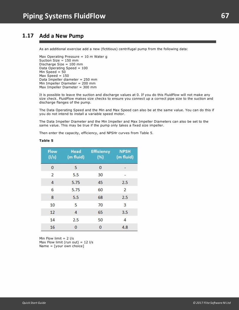
67



1.17 Add a New Pump

As an additional exercise add a new (fictitious) centrifugal pump from the following data:

Max Operating Pressure = 10 m Water gSuction Size = 150 mmDischarge Size = 100 mmData Operating Speed = 100Min Speed = 50Max Speed = 150Data Impeller diameter = 250 mmMin Impeller Diameter = 200 mmMax Impeller Diameter = 300 mm

It is possible to leave the suction and discharge values at 0. If you do this FluidFlow will not make anysize check. FluidFlow makes size checks to ensure you connect up a correct pipe size to the suction anddischarge flanges of the pump.

The Data Operating Speed and the Min and Max Speed can also be at the same value. You can do this ifyou do not intend to install a variable speed motor.

The Data Impeller Diameter and the Min Impeller and Max Impeller Diameters can also be set to thesame value. This may be true if the pump only takes a fixed size impeller.

Then enter the capacity, efficiency, and NPSHr curves from Table 5.

Table 5

Min Flow limit = 2 l/sMax Flow limit (run out) = 12 l/sName = [your own choice]

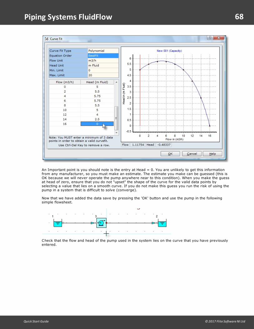
68



An Important point is you should note is the entry at Head = 0. You are unlikely to get this informationfrom any manufacturer, so you must make an estimate. The estimate you make can be guessed (this isOK because we will never operate the pump anywhere near to this condition). When you make the guessat head of zero, ensure that you do not "upset" the shape of the curve for the valid data points byselecting a value that lies on a smooth curve. If you do not make this guess you run the risk of using thepump in a system that is difficult to solve (converge).

Now that we have added the data save by pressing the 'OK' button and use the pump in the followingsimple flowsheet.

Check that the flow and head of the pump used in the system lies on the curve that you have previouslyentered.

69


Index

- A -Activation 4

activation code 4

Add a new pump 67

Add a new Valve 63

Adding new Data 63

Administrator 23

- B -balance the network 31

Balancing 31

boundary 31

building the model 31

- C -calculate button 31

component palette 25

Configuration 59

- D -data entry 31

data input 25

data palette 25, 50

Database 63

Databases 61

default administrator password 23

default data 31

- E -economic pipe size 31

economic velocity 31

Environment 31, 59

environment sets 59

- F -flow balancing 31

Flowsheet 31

fluids database 61

- G -gas collection 50

- H -heat exchanger 31

Help 14

How to enter data 31

How to interpret results 31

How to make changes 31

- I -Inlet Boundary 31

Installation 4, 14

- K -Keeping current 13

known flow boundary 31

known pressure outlet boundary 31

- L -Logon 23

- M -model building basics 31

modules 4

multiple element selections 31

- N -Network 14

network module 21

- O -orifice plates 31

Outlet Boundary 31

70


Index

- P -physical properties 61

physical property prediction methods 61

pipe length 31

pipe numbering 31

pipe size 50

Pipe sizes 31

Pipe Sizing 31

piping network 25

Product Id 4

pump 31, 52

- Q -Quantity 31

quick key 59

- S -schematic layout 25

Setting Up Client 14

settings 59

Setup 4

synchronised 25

System Requirements 4

- W -Welcome 4

Q uick S tar G de - FluidFlo · 4 Q u i c k S t a r t G u i d e ...

Documents

Transcript of Q uick S tar G de - FluidFlo · 4 Q u i c k S t a r t G u i d e ...