Q -Learningsrihari/CSE574/Chap15/15.3-Q-Learning.pdfMachine Learning Srihari Q-Function Property...

Machine Learning Srihari

1

Q - Learning

Sargur N. [email protected]


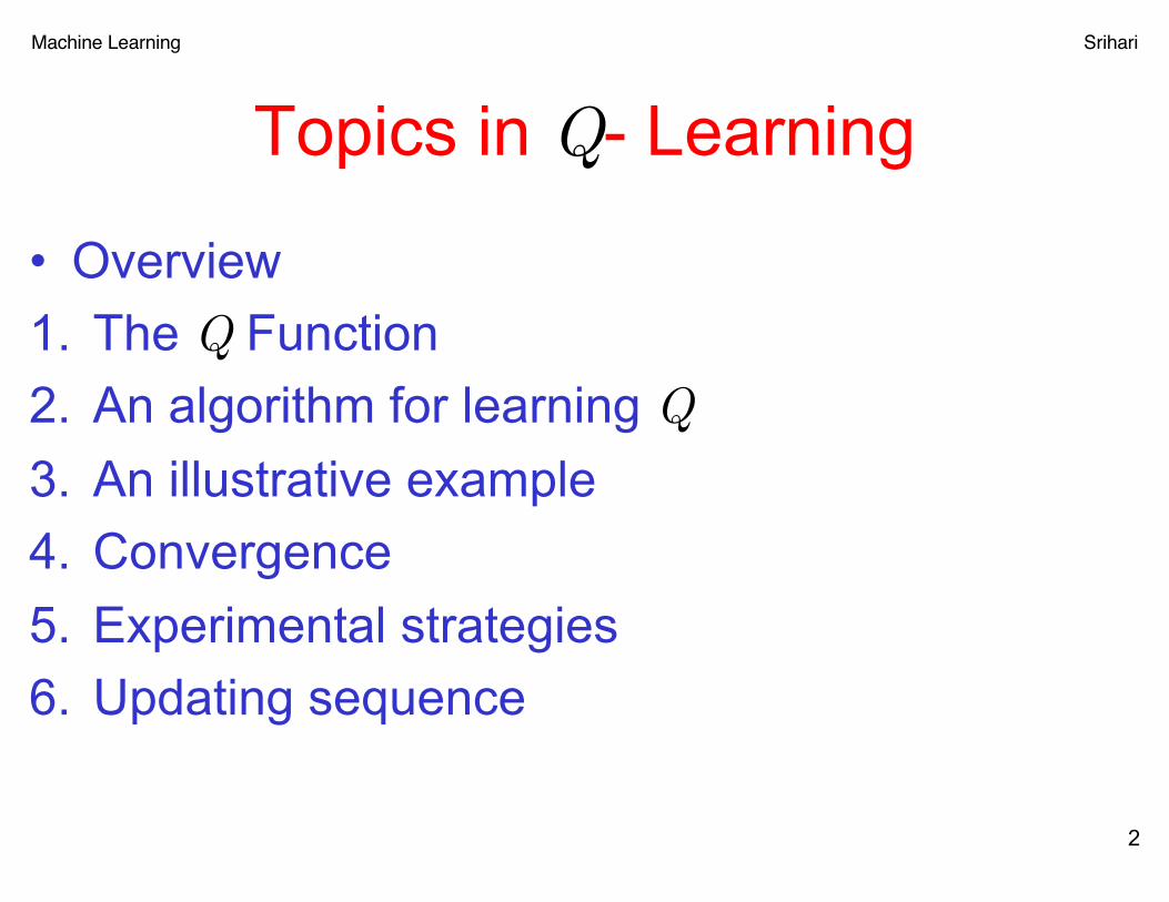
Topics in Q- Learning

• Overview1. The Q Function2. An algorithm for learning Q3. An illustrative example4. Convergence5. Experimental strategies6. Updating sequence

2


Task of Reinforcement Learning

3

Actions aStates s

Task of agent is to learn a policy π: SàA

δ(st,at)=st+1

r(st,at)=rt

st

atrt

st+1


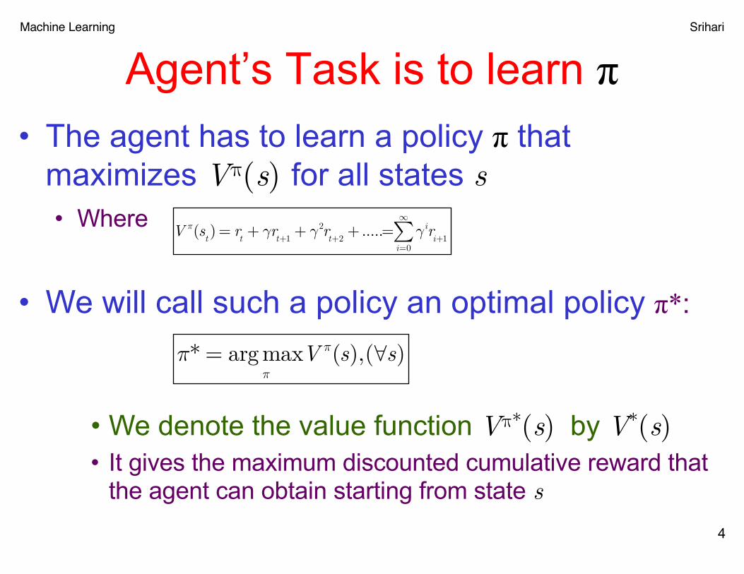
• The agent has to learn a policy π that maximizes Vπ(s) for all states s• Where

• We will call such a policy an optimal policy π*:

• We denote the value function Vπ*(s) by V*(s)• It gives the maximum discounted cumulative reward that

the agent can obtain starting from state s

Agent’s Task is to learn π

4

π* = argmax

πV π(s),(∀s)

V π(s

t) = r

t+ γr

t+1+ γ2r

t+2+ .....= γ ir

i+1i=0

∞

∑


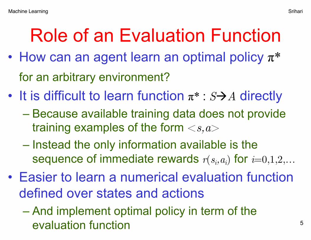
Role of an Evaluation Function• How can an agent learn an optimal policy π*

for an arbitrary environment?• It is difficult to learn function π* : SàA directly

– Because available training data does not provide training examples of the form <s,a>

– Instead the only information available is the sequence of immediate rewards r(si,ai) for i=0,1,2,…

• Easier to learn a numerical evaluation function defined over states and actions– And implement optimal policy in term of the

evaluation function 5


Optimal action for a state• An evaluation function is Vπ*(s) denoted asV* (s)

– where

– Agent prefers s1 over state s2 whenever V*(s1)>V*(s2)• i.e., cumulative feature reward is greater from s1

• Optimal action in state s is the action a– One that maximizes the sum of the immediate

reward r(s,a) plus the value V* of the immediate successor state discounted by γ

• Where δ(s,a) is state resulting from applying action a to s

V π(s

t) = r

t+ γr

t+1+ γ2r

t+2+ .....= γ ir

i+1i=0

∞

∑

π *(s) = argmax

π[r(s,a)+ γV *(δ(s,a))]

π* = argmax

πV π(s),(∀s)


Perfect knowledge of δ and r

• Agent can acquire optimal policy by learning V* provided it has perfect knowledge of– Immediate reward function r, and– State transition function δ– It can then use equation– To calculate the optimal action for any state

• But it may be impossible to predict the outcome of an arbitrary action to an arbitrary state– E.g., robot shoveling dirt when the resulting state

included positions of dirt particles 7

π *(s) = argmax

π[r(s,a)+ γV *(δ(s,a))]


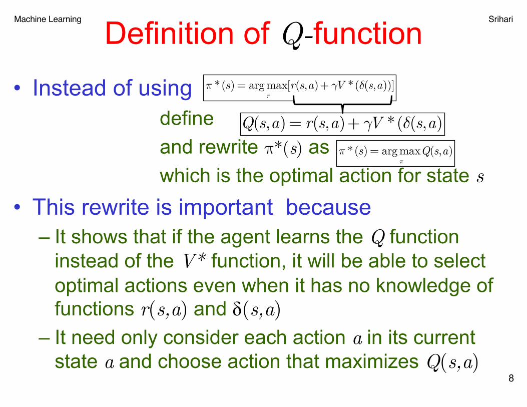
Definition of Q-function• Instead of using

define and rewrite π*(s) as which is the optimal action for state s

• This rewrite is important because– It shows that if the agent learns the Q function

instead of the V* function, it will be able to select optimal actions even when it has no knowledge of functions r(s,a) and δ(s,a)

– It need only consider each action a in its current state a and choose action that maximizes Q(s,a)

8

π *(s) = argmax

π[r(s,a)+ γV *(δ(s,a))]

Q(s,a) = r(s,a)+ γV *(δ(s,a)

π *(s) = argmax

πQ(s,a)


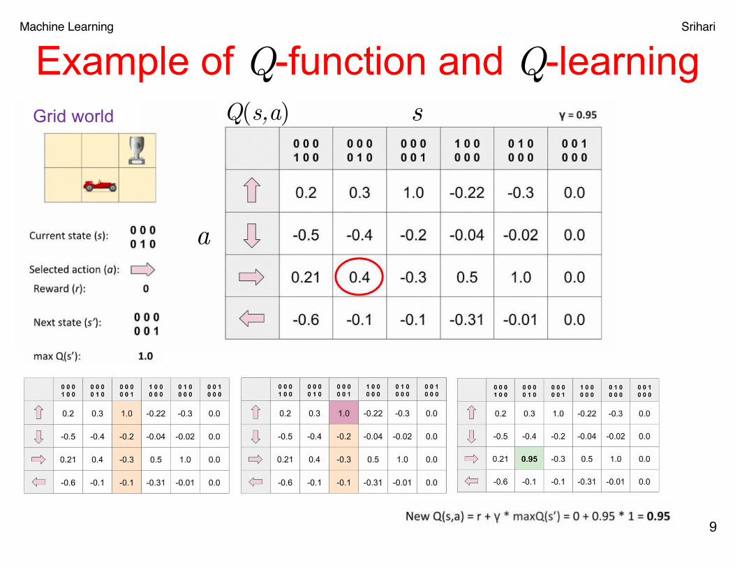
Example of Q-function and Q-learning

9

a

sQ(s,a)Grid world


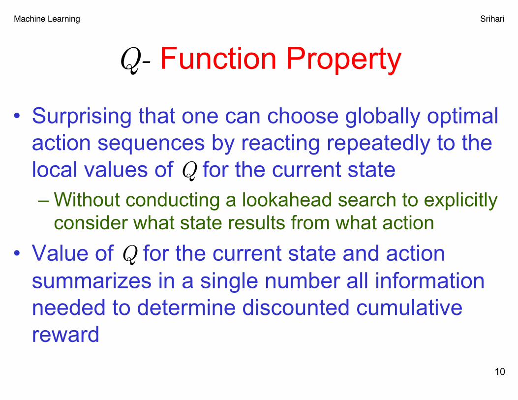
Q- Function Property

• Surprising that one can choose globally optimal action sequences by reacting repeatedly to the local values of Q for the current state– Without conducting a lookahead search to explicitly

consider what state results from what action• Value of Q for the current state and action

summarizes in a single number all information needed to determine discounted cumulative reward

10


An algorithm for learning Q

• Learning the Q function corresponds to learning the optimal policy

• How can Q be learned?• Key problem: finding a reliable way to estimate

training values for Q given only a sequence of immediate rewards r spread out over time

• This can be accomplished through iterative approximation

11


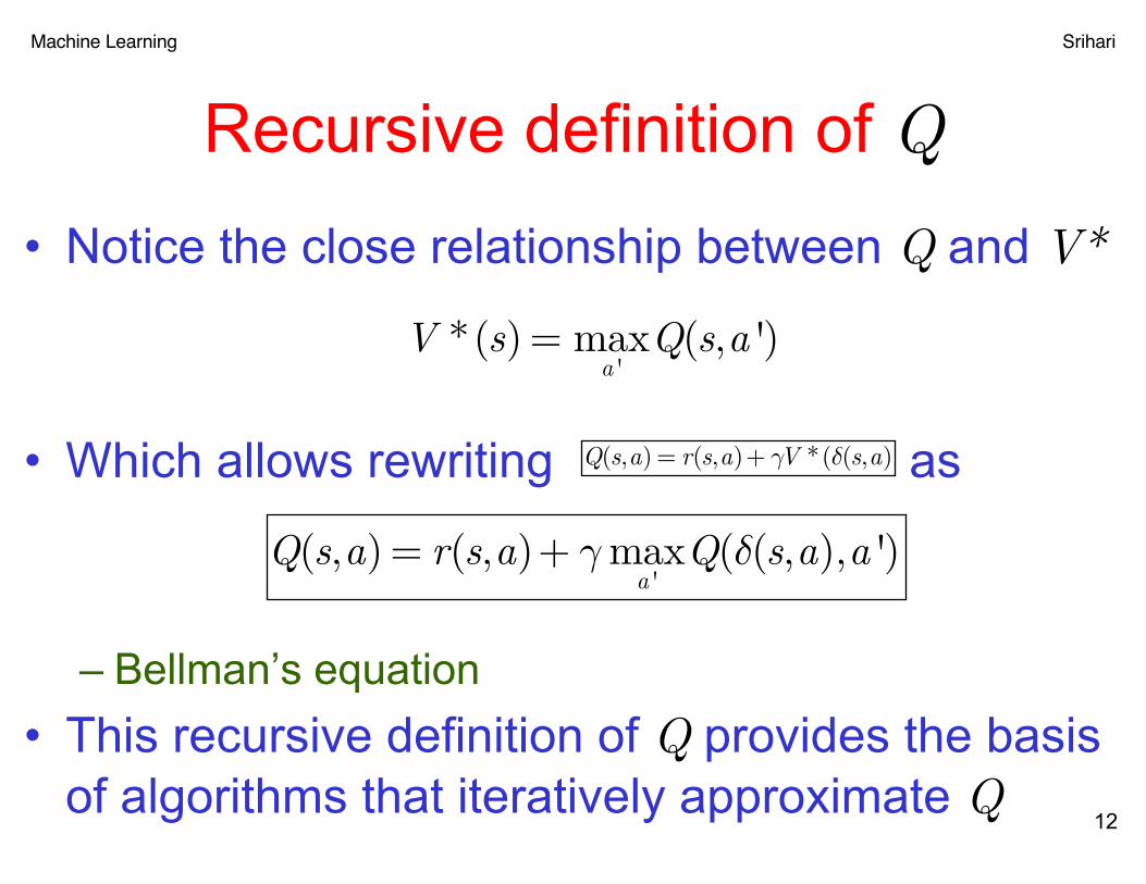
Recursive definition of Q• Notice the close relationship between Q and V*

• Which allows rewriting as

– Bellman’s equation• This recursive definition of Q provides the basis

of algorithms that iteratively approximate Q12

Q(s,a) = r(s,a)+ γV *(δ(s,a)

V *(s) = max

a 'Q(s,a ')

Q(s,a) = r(s,a)+ γmax

a 'Q(δ(s,a),a ')


Table of state-action pairs

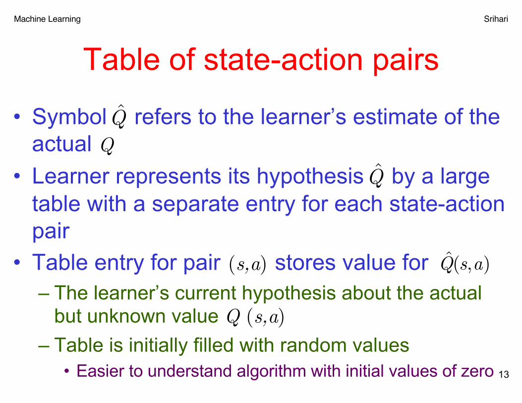
• Symbol refers to the learner’s estimate of the actual Q

• Learner represents its hypothesis by a large table with a separate entry for each state-action pair

• Table entry for pair (s,a) stores value for– The learner’s current hypothesis about the actual

but unknown value Q (s,a)– Table is initially filled with random values

• Easier to understand algorithm with initial values of zero 13

Q̂

Q̂(s,a)

Q̂


Update rule for table entries

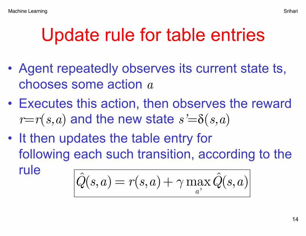
• Agent repeatedly observes its current state ts, chooses some action a

• Executes this action, then observes the reward r=r(s,a) and the new state s’=δ(s,a)

• It then updates the table entry for following each such transition, according to the rule

14

Q̂(s,a) = r(s,a)+ γmax

a 'Q̂(s,a)


Example of updating Q-Learning table

15


Q-learning algorithm for deterministic MDP

• For each s,a initialize the table entry to zero• Observe the current state s• Do forever

– Select an action a and execute it– Receive immediate reward r– Observe the new state s’– Update the table entry for as follows

– sßs’16

Q̂(s,a)

Q̂(s,a)← r + γmax

a 'Q̂(s ',a ')

Q̂(s,a)


Q-Learning for Atari Breakout

17

https://www.youtube.com/watch?v=V1eYniJ0Rnk&vl=en

https://www.youtube.com/watch?v=V1eYniJ0Rnk&vl=en

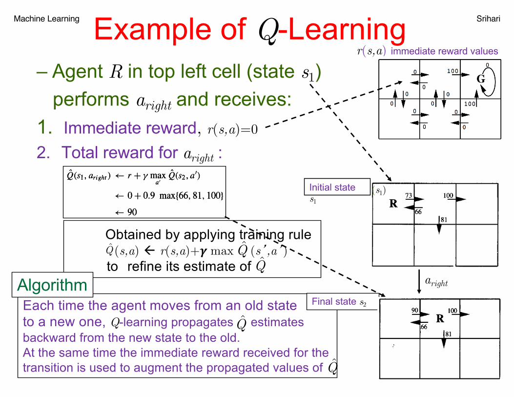
Machine Learning SrihariExample of Q-Learning– Agent R in top left cell (state s1)

performs aright and receives:1. Immediate reward, r(s,a)=0

2. Total reward for aright :

r(s,a) immediate reward values

(s1)

Obtained by applying training rule (s,a) ß r(s,a)+! max (s�,a�)

to refine its estimate of Q̂ Q̂ Q̂

(s2)

Initial state s1

aright

Each time the agent moves from an old stateto a new one, Q-learning propagates estimatesbackward from the new state to the old.At the same time the immediate reward received for thetransition is used to augment the propagated values of

Q̂

Q̂

Final state s2Algorithm


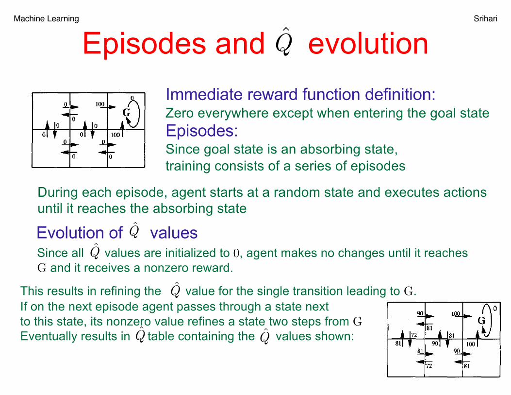
Episodes and evolution

19

Immediate reward function definition: Zero everywhere except when entering the goal stateEpisodes:Since goal state is an absorbing state, training consists of a series of episodes

During each episode, agent starts at a random state and executes actionsuntil it reaches the absorbing state

Evolution of values Q̂

Q̂

Since all values are initialized to 0, agent makes no changes until it reachesG and it receives a nonzero reward.

Q̂

This results in refining the value for the single transition leading to G.If on the next episode agent passes through a state nextto this state, its nonzero value refines a state two steps from GEventually results in table containing the values shown:

Q̂

Q̂ Q̂


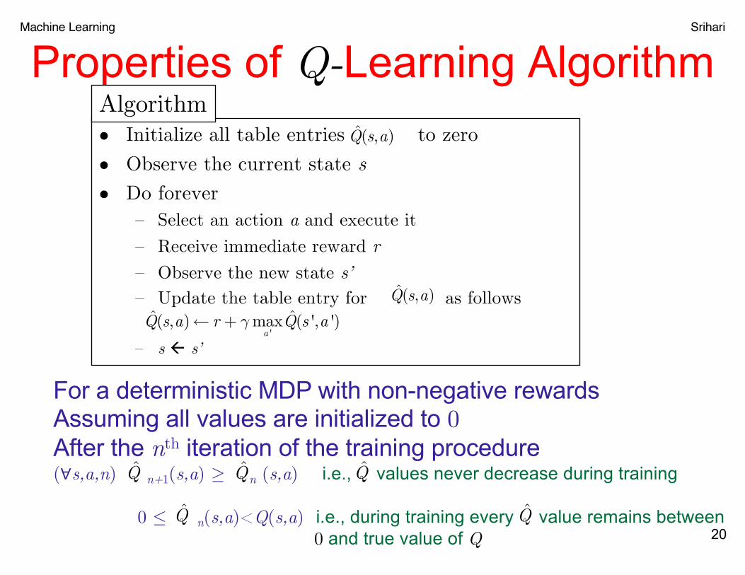
Properties of Q-Learning Algorithm

20

• Initialize all table entries to zero

• Observe the current state s• Do forever

– Select an action a and execute it

– Receive immediate reward r– Observe the new state s’– Update the table entry for as follows

– s ß s’

Q̂(s,a)

Q̂(s,a)← r + γmax

a 'Q̂(s ',a ')

Q̂(s,a)

For a deterministic MDP with non-negative rewardsAssuming all values are initialized to 0After the nth iteration of the training procedure(∀s,a,n) n+1(s,a) ≥ n (s,a) i.e., values never decrease during training

0 ≤ n(s,a)<Q(s,a) i.e., during training every value remains between0 and true value of Q

Q̂ Q̂

Q̂

Algorithm

Q̂

Q̂


Convergence of Algorithm

• Q-Learning algorithm converges towards a equal to Q under the following conditions:1. Deterministic MDP2. Immediate reward values are bounded r(s,a)<c3. Agent visits every possible state-action pair

infinitely• Q-Learning convergence theorem is formally

stated next

21

Q̂


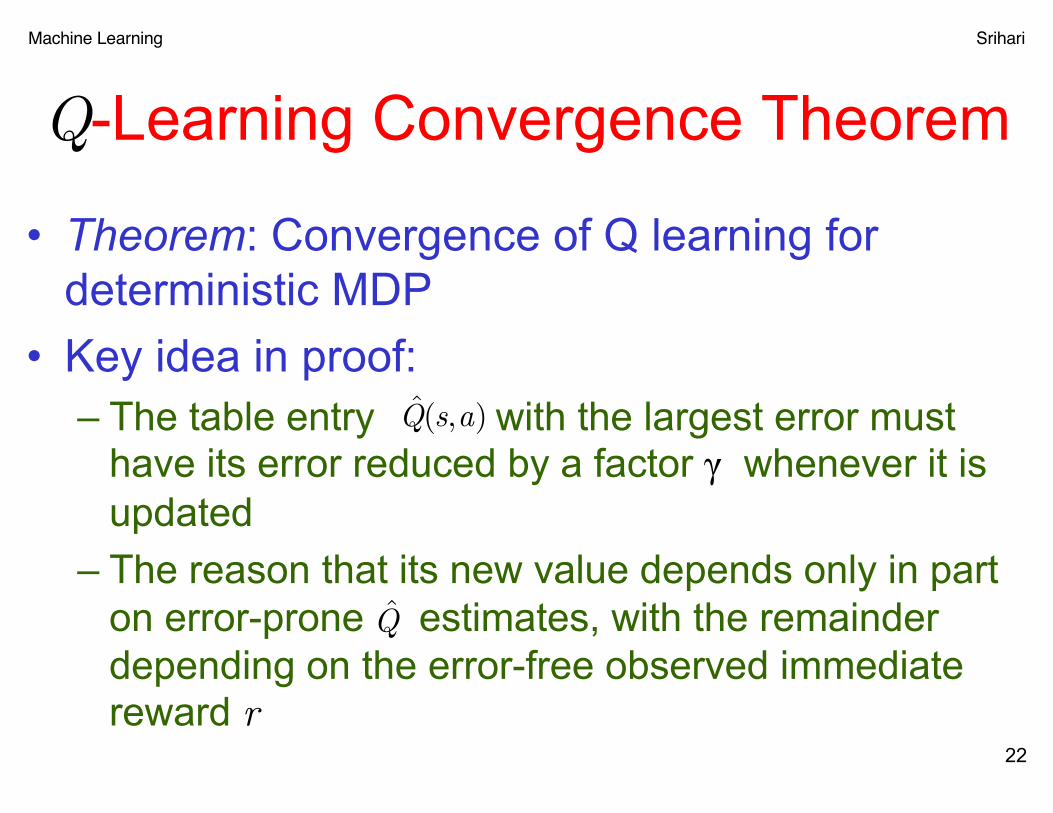
Q-Learning Convergence Theorem

• Theorem: Convergence of Q learning for deterministic MDP

• Key idea in proof:– The table entry with the largest error must

have its error reduced by a factor γ whenever it is updated

– The reason that its new value depends only in parton error-prone estimates, with the remainder depending on the error-free observed immediate reward r

22

Q̂(s,a)

Q̂


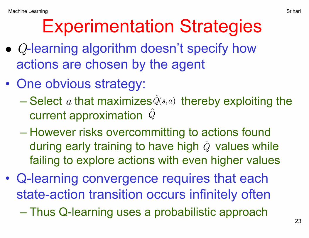
Experimentation Strategies• Q-learning algorithm doesn’t specify how

actions are chosen by the agent• One obvious strategy:

– Select a that maximizes thereby exploiting the current approximation

– However risks overcommitting to actions found during early training to have high values while failing to explore actions with even higher values

• Q-learning convergence requires that eachstate-action transition occurs infinitely often– Thus Q-learning uses a probabilistic approach

23

Q̂(s,a)

Q̂

Q̂


Exploitation and Exploration• Probability of action ai is

• Larger values of k will assign higher probabilities to actions with above average – causing the agent to exploit what it has learned

and seek actions it believes will maximize its reward• Small values of k will allow higher probabilities

for other actions, leading the agent– to explore actions that do not currently have high

values. 24

Q̂

Q̂


From exploitation to exploration

• k is varied with the number of iterations • So that the agent favors exploration during

early stages of learning • Then gradually shifts toward a strategy of

exploitation

25


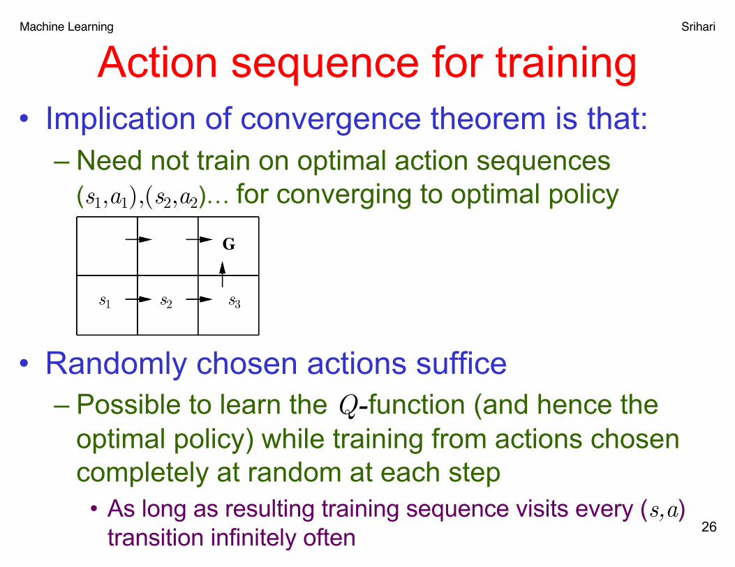
Action sequence for training• Implication of convergence theorem is that:

– Need not train on optimal action sequences (s1,a1),(s2,a2)… for converging to optimal policy

• Randomly chosen actions suffice– Possible to learn the Q-function (and hence the

optimal policy) while training from actions chosen completely at random at each step• As long as resulting training sequence visits every (s,a)

transition infinitely often 26

s1 s2 s3


Action Sequences for Efficiency

• Since any action sequence suffices– We can change sequences of training example

transitions • to improve training efficiency without endangering final

convergence

• How to determine such sequences?

27


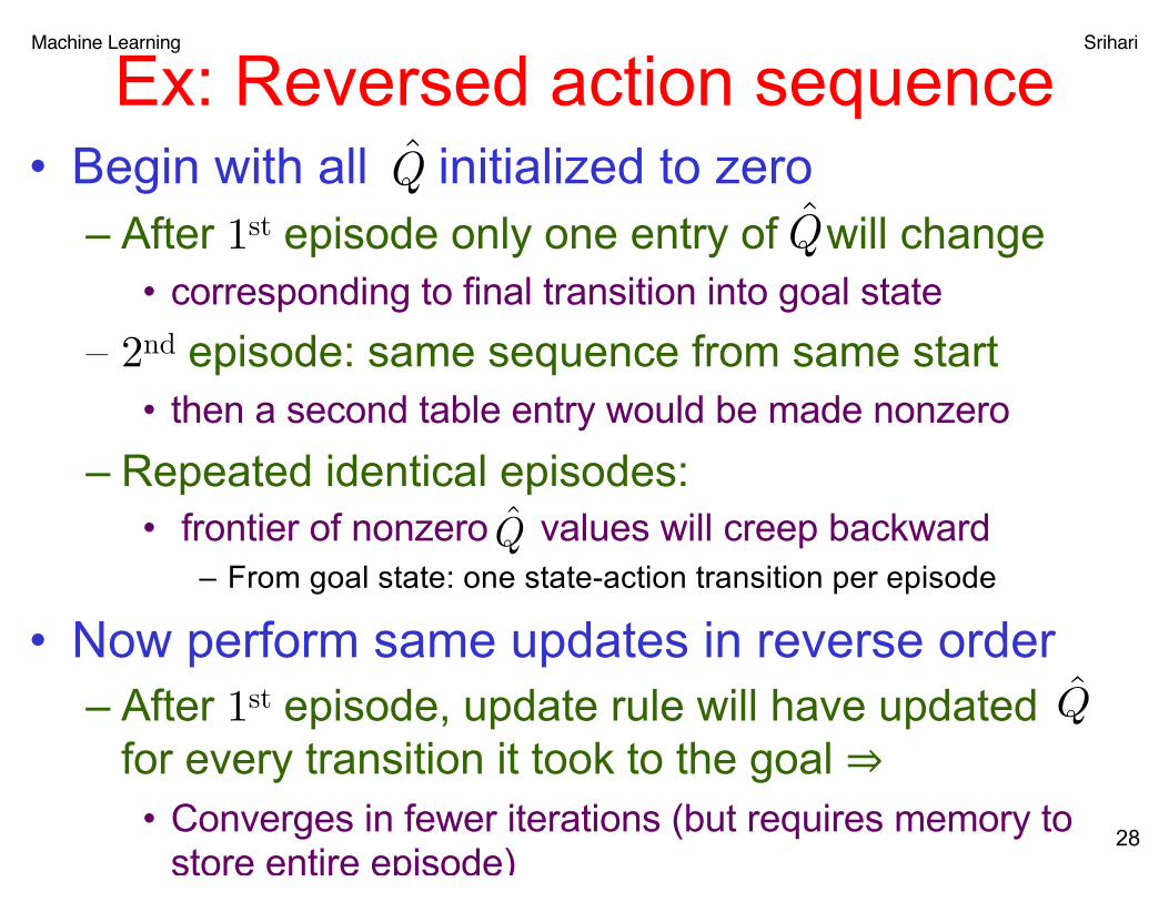
Ex: Reversed action sequence • Begin with all initialized to zero

– After 1st episode only one entry of will change• corresponding to final transition into goal state

– 2nd episode: same sequence from same start • then a second table entry would be made nonzero

– Repeated identical episodes:• frontier of nonzero values will creep backward

– From goal state: one state-action transition per episode

• Now perform same updates in reverse order– After 1st episode, update rule will have updated

for every transition it took to the goal ⇒• Converges in fewer iterations (but requires memory to

store entire episode)28

Q̂

Q̂

Q̂

Q̂


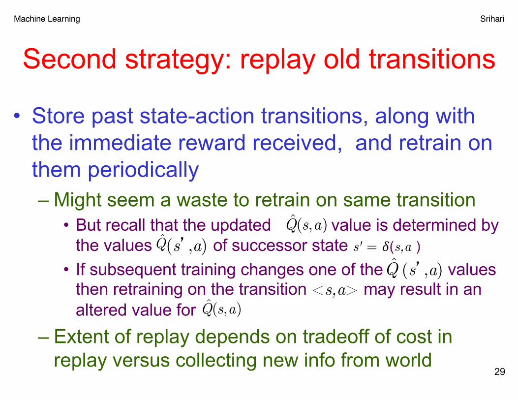
Second strategy: replay old transitions

• Store past state-action transitions, along with the immediate reward received, and retrain on them periodically – Might seem a waste to retrain on same transition

• But recall that the updated value is determined by the values (s�,a) of successor state s' = !(s,a )

• If subsequent training changes one of the (s�,a) values then retraining on the transition <s,a> may result in an altered value for

– Extent of replay depends on tradeoff of cost in replay versus collecting new info from world

29

Q̂(s,a)

Q̂

Q̂(s,a)

Q̂

Q -Learningsrihari/CSE574/Chap15/15.3-Q-Learning.pdfMachine Learning Srihari Q-Function Property...

Documents

Transcript of Q -Learningsrihari/CSE574/Chap15/15.3-Q-Learning.pdfMachine Learning Srihari Q-Function Property...