PSCAD: Power System Simulationforum.hvdc.ca/DownloadFile.aspx?file=UserFiles... · PSCAD® 4.2 PART...

Copyright – January 2006

PSCAD: Power System Simulation

PSCAD®

Version 4.2

WIND TURBINE APPLICATIONS TECHNICAL PAPER

PSCAD is a registered trademark.

PSCAD software COPYRIGHT MANITOBA HVDC Research Centre Inc. PSCAD tutorials COPYRIGHT CEDRAT

This technical paper was edited 9 January 2006 Ref.: KP05-A-EN-01/06

CEDRAT 15 Chemin de Malacher- Inovallée

38246 MEYLAN Cedex FRANCE

Phone: +33 (0)4 76 90 50 45 Fax: +33 (0)4 56 38 08 30 Email: [email protected]

Web: www.cedrat.com

PSCAD® 4.2 Introduction

TABLE OF CONTENTS

PART A: INTRODUCTION 1

1. Introduction ..................................................................................................................3

2. PSCAD components....................................................................................................5

3. Modelled structure .......................................................................................................7

4. Simulations performed.................................................................................................9

PART B: BUILD THE MODEL 11

5. From the wind to the Synchronous Generator ...........................................................13 5.1 The Wind Source.........................................................................................................14 5.2 The wind turbine component .......................................................................................15

5.2.1 Theoretical study ...................................................................................................15 5.2.2 Cp curve with PSCAD standard model .................................................................16 5.2.3 Computation of parameters...................................................................................17 5.2.4 Define the Wind turbine parameters .....................................................................18

5.3 Wind turbine governor component ..............................................................................19 5.3.1 Theoretical study ...................................................................................................19 5.3.2 Define the Wind governor parameters ..................................................................20

5.4 The synchronous generator.........................................................................................21 5.5 Turbine generator connection: Simulation at rated load..............................................24

Simulation parameters & analysis : ......................................................................................24

6. AC/DC/AC : Power and Frequency conversion .........................................................27 6.1 Diode Rectifier .............................................................................................................28 6.2 Overvoltage protection ................................................................................................30 6.3 DC bus.........................................................................................................................31

6.3.1 Build the DC bus....................................................................................................31 6.3.2 Model validation.....................................................................................................32

6.4 6-Pulse Thyristor inverter ............................................................................................34

WIND TURBINE APPLICATIONS PAGE A

PSCAD®4.02 Introduction

6.4.1 Presentation.......................................................................................................... 34 6.4.2 Voltage collapse limitation .................................................................................... 36 6.4.3 Voltage regulation................................................................................................. 37

6.5 Connection to the network ..........................................................................................40

7. The distribution grid ...................................................................................................43 7.1.1 Definition of the grid.............................................................................................. 43 7.1.2 Load Flow Simulation ........................................................................................... 47

PART C: SIMULATE 49

8. Constant Wind Study .................................................................................................51 8.1 Structure the complete model .....................................................................................51 8.2 Constant wind study....................................................................................................53

9. Fault Analysis.............................................................................................................55 9.1 Default at Node 3 ........................................................................................................56

9.1.1 Without DG ........................................................................................................... 56 9.1.2 With DG connected at node 1 .............................................................................. 57

9.2 Default at Node 2 ........................................................................................................59 9.2.1 Without DG ........................................................................................................... 59 9.2.2 With DG connected at node 3 .............................................................................. 59

9.3 Conclusion ..................................................................................................................61

10. Variable wind study....................................................................................................63 10.1 Dynamic pitch control ..................................................................................................63 10.2 Passive pitch control simulation ..................................................................................67 10.3 Comparison of passive and dynamic pitch control ......................................................69

11. Wind farm...................................................................................................................71 11.1 From a single wind turbine to a wind farm ..................................................................72

11.1.1 Change the structure of the model ....................................................................... 72 11.1.2 Modifications in the synchronous generator......................................................... 73 11.1.3 Modifications in the transformer ........................................................................... 74 11.1.4 Modifications in the grid........................................................................................ 74

11.2 PWM Regulation drives...............................................................................................75 11.2.1 Principles .............................................................................................................. 75 11.2.2 Generation of the triangular waveform ................................................................. 75 11.2.3 Generation of the reference.................................................................................. 79 11.2.4 Generation of the firing pulses for the GTO inverter ............................................ 83

11.3 Simulation 85

PART D: APPENDIX 87

12. References.................................................................................................................89

PAGE B WIND TURBINE APPLICATIONS

PSCAD® 4.2 PART A: INTRODUCTION Introduction

PART A: INTRODUCTION

WIND TURBINE APPLICATIONS PAGE 1

PART A: INTRODUCTION PSCAD®4.02 Introduction

PAGE 2 WIND TURBINE APPLICATIONS

PSCAD® 4.2 PART A: INTRODUCTION Introduction

1. Introduction

Recently, wind power generation has attracted special interest, and many wind power stations are in service throughout the world. In wind power stations, induction machines are often used as generators, but the development of new permanent magnet generators, the improvement of the AC-DC-AC conversion and its advantages for output power quality make other solutions possible. A recent solution is to use a permanent magnet generator with variable speed and a conversion stage, which is the case studied in this technical paper. The aim of this tutorial is to familiarize users with PSCAD software through a complete example. PSCAD contains powerful tools for the wind turbine simulation. Part B describes the step-by-step building of the entire energy generation cycle for one wind turbine. All components are dimensioned and connected to each other. Intermediate simulations validate the model. In Part C, different power turbine regulation types are simulated and analyzed, and fault situations on the grid are studied. Finally, an entire wind farm is modelled.


PART A: INTRODUCTION PSCAD®4.02 Introduction


PSCAD® 4.2 PART A: INTRODUCTION PSCAD components

2. PSCAD components

In PSCAD, the complete wind generator cycle is composed of : The wind source component:

VwESWind Source

GustMean

Ramp

• The mechanical turbine, represented by a component called “wind turbine”.

TmVw

Beta

W P

Wind TurbineMOD 2 Type

• The regulation governor of the turbine’s output power. This regulation can be passive (passive

pitch control) or dynamic (dynamic pitch control). The difference is whether or not the blades turn around their longitudinal axis. Both kinds of regulation can be simulated by a component called “Wind turbine governor”.

Wind TurbineGovernor

Wm

Beta

PgMOD 2 Type

• The other components are standard ones: synchronous machine, transformer, rectifier, inverter,

Control System, Modelling Functions (CSMF),…. All these components will be detailed in Part B.


PART A: INTRODUCTION PSCAD®4.02 PSCAD components


PSCAD® 4.2 PART A: INTRODUCTION Modelled structure

3. Modelled structure

Part B contains: • A theoretical study of wind turbine generation • The dimensioning of each PSCAD component with intermediate simulations in order to compare

results with the theory and to validate the model. This paper makes the choice to define a wind turbine connected to a permanent Magnet Synchronous Generator with 100 pole pairs. The connection to the grid is then performed through a full AC/DC/AC converter and a step up transformer. The main advantage of this strategy is to allow to remove the gear box in the wind turbine. Of course different technologies can be fully simulated in PSCAD:

o Induction generatore direct connection o Doubly Fed Induction Generator

Some examples of the implementation of this models in PSCAD can be asked to CEDRAT or your local PSCAD distributor. In this document, the overall sequence can be summarized by the following diagram:


PART A: INTRODUCTION PSCAD®4.02 Modelled structure


PSCAD® 4.2 PART A: INTRODUCTION Simulations performed

4. Simulations performed

In part C, the global sequence is achieved through the connection of all components presented in part B and the simulation results are analyzed: • The power produced with a constant mean wind speed (13 m/s)

• The power produced with variable wind speed and passive pitch control

• The power produced with variable speed and dynamic pitch control

• The differences between the two types of pitch control • The wind turbine’s impact on a distribution network in case of faults on the network

• The wind farm model and the impact of a wind farm connection on a transmission network


PART A: INTRODUCTION PSCAD®4.02 Simulations performed


PSCAD® 4.0 PART B: BUILD THE MODEL Simulations performed

PART B: BUILD THE MODEL


PART B: BUILD THE MODEL PSCAD®4.0 Simulations performed


PSCAD® 4.0 PART B: BUILD THE MODEL From the wind to the Synchronous Generator

5. From the wind to the Synchronous Generator

In the first sections ( 5.1 to 5.5) , the following components will be described and dimensioned: • Wind Source component • Wind Turbine component • Wind Governor • Synchronous Generator Then, a first simulation will be done to check the dimensioning. First create a new PSCAD project : Turbine_generator.psc In the project Settings, enable the unit conversion system (available in PSCAD 4.2) to have the possibility to use different units than PSCAD default units:


PART B: BUILD THE MODEL PSCAD®4.0 From the wind to the Synchronous Generator

5.1 The Wind Source

VwESWind Source

GustMean

Ramp

I / O Definition Description ES Input

External value An external value created by the user can be added to the value

internally generated. Vw Output

Wind Speed (m/s) Wind speed in m/s.

Table 1: INPUT / OUTPUT for wind source component This component can be found in the folder “Master Library/Machines”. The Wind Source component simulates every wind condition: • mean wind speed • periodic gust with a sinus form • ramp • noise • damper for all the preceding conditions For wind turbine, the three following wind characteristics are important: • The mean wind speed:

The rated characteristics of the turbine and the generator are determined according to the mean wind speed. Economic studies are also based on this speed. In general, the mean wind speed is approximately 13 m/s.

• The cut-in speed: At speeds higher than the cut-in speed, mechanical brakes are released in order to let the turbine turn. In general, the cut-in speed is equal to 4 m/s.

• The cut-out speed: At speeds higher than the cut-out speed, the turbine rotation is stopped in order not to damage the blades of the turbine. In general, the cut-out speed is approximately 25 m/s.

For dynamic simulations, the wind speed is simulated throughout a day; thus, the wind speed must vary from the cut-in speed to the cut-out speed in order to study the wind turbine’s reaction for all wind conditions. In this study, a startup below the cut-in speed and a stop above the cut-out speed are not considered; the wind speed is limited to between 4m/s and 25m/s. First, we will consider a constant wind at 13m/s. Copy a wind source component in your project and parameterize it as shown in Figure 1:

Figure 1: Wind source characteristics



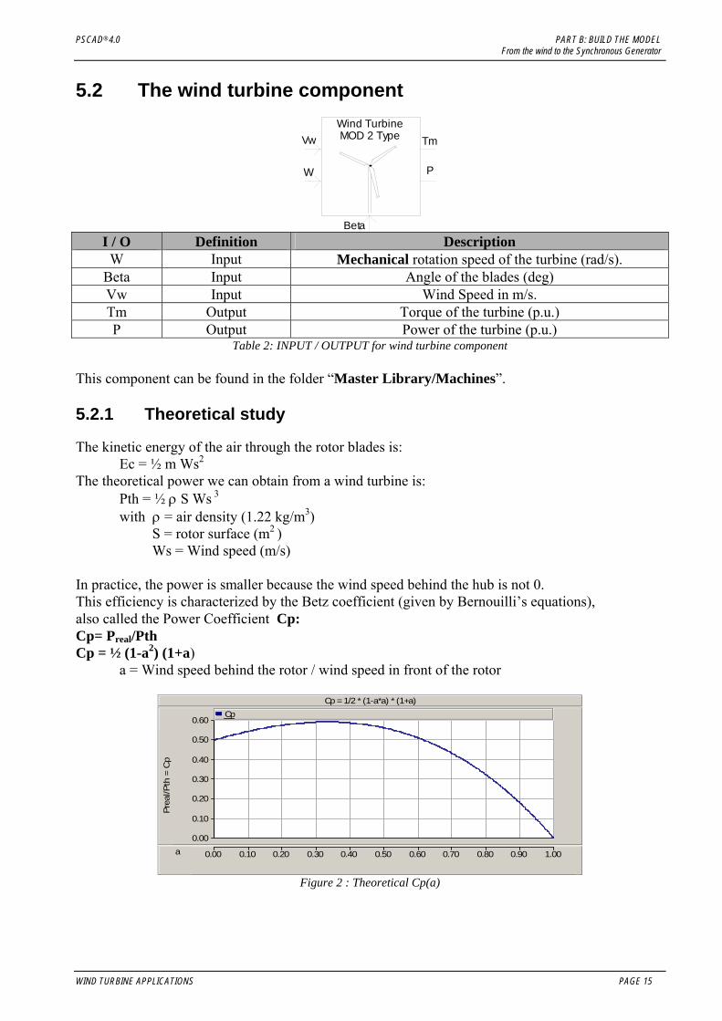
5.2 The wind turbine component

TmVw

Beta

W P


I / O Definition Description

W Input Mechanical rotation speed of the turbine (rad/s). Beta Input Angle of the blades (deg) Vw Input Wind Speed in m/s. Tm Output Torque of the turbine (p.u.) P Output Power of the turbine (p.u.)

Table 2: INPUT / OUTPUT for wind turbine component This component can be found in the folder “Master Library/Machines”.

5.2.1 Theoretical study

The kinetic energy of the air through the rotor blades is: Ec = ½ m Ws2 The theoretical power we can obtain from a wind turbine is: Pth = ½ ρ S Ws 3

with ρ = air density (1.22 kg/m3) S = rotor surface (m2 ) Ws = Wind speed (m/s)

In practice, the power is smaller because the wind speed behind the hub is not 0. This efficiency is characterized by the Betz coefficient (given by Bernouilli’s equations), also called the Power Coefficient Cp: Cp= Preal/Pth Cp = ½ (1-a2) (1+a)

a = Wind speed behind the rotor / wind speed in front of the rotor

Cp = 1/2 * (1-a*a) * (1+a)

a 0.00 0.10 0.20 0.30 0.40 0.50 0.60 0.70 0.80 0.90 1.00 ...

0.00

0.10

0.20

0.30

0.40

0.50

0.60

Prea

l/Pth

= C

p

Cp

Figure 2 : Theoretical Cp(a)



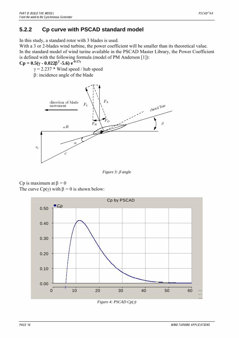
5.2.2 Cp curve with PSCAD standard model

In this study, a standard rotor with 3 blades is used. With a 3 or 2-blades wind turbine, the power coefficient will be smaller than its theoretical value. In the standard model of wind turine available in the PSCAD Master Library, the Power Coefficient is defined with the following formula (model of PM Anderson [1]): Cp = 0.5(γ - 0.022β2 -5.6) e-0.17γ

γ = 2.237 * Wind speed / hub speed β: incidence angle of the blade

Figure 3: β angle

Cp is maximum at β = 0 The curve Cp(γ) with β = 0 is shown below:

Cp by PSCAD

0 10 20 30 40 50 60 ... ... ...

0.00

0.10

0.20

0.30

0.40

0.50 Cp

Figure 4: PSCAD Cp(γ)



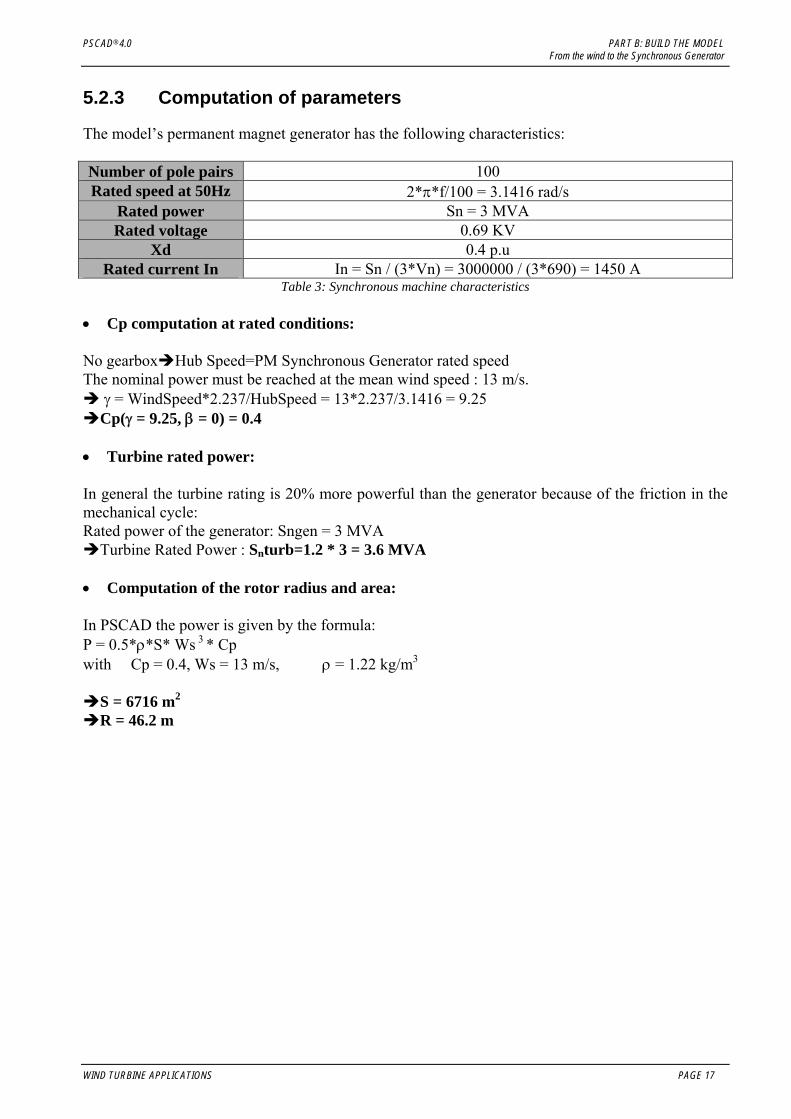
5.2.3 Computation of parameters

The model’s permanent magnet generator has the following characteristics: Number of pole pairs 100 Rated speed at 50Hz 2*π*f/100 = 3.1416 rad/s

Rated power Sn = 3 MVA Rated voltage 0.69 KV

Xd 0.4 p.u Rated current In In = Sn / (3*Vn) = 3000000 / (3*690) = 1450 A

Table 3: Synchronous machine characteristics • Cp computation at rated conditions: No gearbox Hub Speed=PM Synchronous Generator rated speed The nominal power must be reached at the mean wind speed : 13 m/s.

γ = WindSpeed*2.237/HubSpeed = 13*2.237/3.1416 = 9.25 Cp(γ = 9.25, β = 0) = 0.4

• Turbine rated power: In general the turbine rating is 20% more powerful than the generator because of the friction in the mechanical cycle: Rated power of the generator: Sngen = 3 MVA

Turbine Rated Power : Snturb=1.2 * 3 = 3.6 MVA • Computation of the rotor radius and area: In PSCAD the power is given by the formula: P = 0.5*ρ*S* Ws 3 * Cp with Cp = 0.4, Ws = 13 m/s, ρ = 1.22 kg/m3

S = 6716 m2

R = 46.2 m



5.2.4 Define the Wind turbine parameters

Copy a wind turbine component in your case and define its parameter as following:

Figure 5: Wind turbine characteristics



5.3 Wind turbine governor component


Wm

Beta

PgMOD 2 Type

I / O Definition Description Wm Input Mechanical rotation speed of the turbine (rad/s). Pg Input Output power of the turbine (p.u.)

Beta Output Angle of the blades (deg) Table 4: INPUT / OUTPUT for Wind governor

This component can be found in the library “Master Library/Machines”.

5.3.1 Theoretical study

Cp = 0.5(γ - 0.022β2 -5.6) e-0.17γ

The regulation of β enables the regulation of Cp and thus enables to control the output power of the turbine depending on wind conditions. Two regulation strategies exists and are described below: • Passive pitch control: The β angle is determined by the wind turbine builder to produce maximum energy for a predefined average speed. Below the mean wind speed, there is no angle control: Cp is not maximum. Above the mean wind speed, the blade profile creates turbulence in order to keep the rotation of the blades from increasing. • Dynamic pitch control: In this configuration, the blades can turn around their longitudinal axis. A power reference for the regulation system is given, and at each second the system turns the blades in order to regulate the output power as shown on the following curve:

Figure 6: P(V) characteristic

• Zone I: Vwind < Vcut-in P = 0 (the turbine does not turn) • Zone II: P<Prated P = f(V) with β = 0 • Zone III: P = Prated with β ≠ 0, P is kept at Prated through the dynamic pitch control • Zone IV: Vwind > Vcut-out P = 0 (The turbine is stopped with mechanical brakes)



5.3.2 Define the Wind governor parameters

Copy a wind governor component in your case and define its parameter as following::

PSCAD can simulate a 2 or 3blades wind turbine.MOD2 defines a 3 blades windturbine.There is no gear box.

The regulation must provide therated power at the rated speed.

The wind turbine governorallows also to regulate the windspeed. As we use the powerregulation, these parameters mustbe set to 0

The start is done with hmaximum power

( Beta = 0 ).

The blades can rotate from0 deg to 25 deg.

Figure 7: Governor characteristics



5.4 The synchronous generator The synchronous generator is described with the following component:

Sync1

w

Te

A

B

C

IfEfEf If

TmTm

I / O Definition Description Ef Input The exciter voltage (p.u.) Tm Input, output The mechanical torque (p.u.) If Output The exciter current (p.u.) Te Output The electrical torque (p.u.) w Output The speed of the generator (p.u.)

A,B,C Output The voltage (KV) Table 5: INPUT / OUTPUT Synchronous generator

The synchronous generator component can be found in the folder “Master Library/Machines”. • Computation of parameters: In this study we use a permanent magnet generator, so the excitation is constant and equal to 1 p.u.: Number of pole pairs 100 Rated speed at 50Hz 2*π*f/100 = 3.1416 rad/s

Rated power Sn = 3 MVA Rated voltage 0.69 KV

Xd 0.4 p.u Rated current In In = Sn / (3*Vn) = 3000000 / (3*690) = 1450 A

Table 6: Synchronous machine characteristics

Note: 1. p.u values: In PSCAD all the internal values are defined in p.u. Therefore, a new rated

value will modify all the internal parameters, the user does not need to calculate all the new values.

2. Synchronous machine starting in PSCAD: PSCAD enables starting the simulation with the generator as a source or with the rotor speed constant. In this study, the startup is done with the mean wind speed and with the initial machine speed.

3. Modeling of a permanent magnet generator: To model a PM synchronous generator with a classical synchronous model we have chosen: • A constant excitation voltage: 1 p.u. • A large unsaturated transient time Tdo′, which increases the field leakage: 10 s • A very small unsaturated subtransient time Tdo″, which simulates the effect of a large

damper resistance: 0.0001s • An initial Field current equal to its permanent value



Copy a synchronous generator component in your case and define its parameter as following:

Figure 8: Synchronous machine characteristics



The permanent magnetscreate the following startingconditions because the fieldis constant all the time andthus before the start of thesimulation

Figure 9: Synchronous machine characteristics



5.5 Turbine generator connection: Simulation at rated load Now connect all the components as below:

Figure 10: Turbine-generator connection

Note: Computation of the rated load Wind speed = rated value = 13 m/s β is forced to 0 in order to have the maximum power and The wind turbine delivers 3.6 MW:

P = 3*V*I*cosϕ = 3*V2*R/ Z2 = 3*V2*R / (R2 + Xd2) with Xd = 0.4 pu = 0.4* Vn/In = 0.4 * 690/1450 = 0.19 Ω

The rated load of the generator is: R = 0.257 Ω.

Simulation parameters & analysis :

• Duration: 40s • Time step: 100 µs • Plot step: 1000µs • Startup method: Standard • Scale Factors ( to display T and P with real values and non pu values)

Variable Name Scale FactorPgene 3Qgene 3Pturb 3

Wmech 1Tturb 955000

T_elec_gen 955000 Table 7: Scale Factors for measured quantities



The evolution of curves follows the fundamental mechanical law: • Turbine Torque – Electromagnetic Torque = J*dw/dt + f*w

during the starting, the Turbine torque is > To the Electromagnetic Torque: Speed increases. • Turbine power is managed by the Cp value, which is a wind speed and a hub speed function. In this example the wind speed is constant (13 m/s), thus, Cp is only a hub speed function. As the speed increases, the power coefficient Cp = 0.5(γ - 0.022β2 -5.6) e-0.17γ decreases.

Turbine power decreases • Final steady state : Turbine Torque – Electromagnetic Torque = f*w Tturb = 1 173 000 Nm TelecGene = 1 156 000 Nm

f*w = 1 173 000 – 1 156 000 = 17 000 Nm w = 3.06 rad/s and f = 0.02 pu = 0.02 * 955000 = 19100 Nm

f*w = 19100 * 3.06 / 3.14 = 18 600 Nm ≅17000 Nm

• The turbine power corresponds to the rated power (3.6 MW) • The generator power starts from 0 to the turbine rated power • The speed is approximately the rated speed (3.06 rad/s)

Figure 11: Curves obtained with “turb_gen_connection.psc”


PSCAD® 4.0 PART B: BUILD THE MODEL AC/DC/AC : Power and Frequency conversion

6. AC/DC/AC : Power and Frequency conversion

The speed of the wind source being variable, a converter stage AC-DC-AC must be implemented in order to connect the output of the synchronous generator (variable frequency and voltage) to the grid, where a constant frequency and a constant voltage is needed. In the following parts, the power conversion stage will be described and parameterized. It is composed of a :

o A diode rectifier o A DC bus with a storage capacitance voltage o A 6-pulse bridge thyristor inverter

As the model represents only a single wind turbine, the firing angle of the thyristor are not controlled functions of the voltage level at the grid connection point but to keep the DC bus voltage to its rated level +/- 10%. This will involve the modelling of HVDC control systems as shown in the following parts.


PART B: BUILD THE MODEL PSCAD®4.0 AC/DC/AC : Power and Frequency conversion

6.1 Diode Rectifier A 3 phase diode-rectifier can be modelled in PSCAD with the following component:

I / O Definition Description ComBus Input The reference for the conduction start (V)

KB Input Block / deblock control signals (0,1) A0 Input Firing angle from the reference (rad or deg)

A,B,C Input The alternating voltage AM Output Firing angle measurement (rad or deg) GM Output Extinction angle measurement (rad or deg)

Output The direct voltage (KV) Table 8: INPUT / OUTPUT rectifier – inverter

The 6pulse_bridge component can be found in the folder “Master Library/HVDC&FACTS”. Copy the generator and turbine in a subpage then connect it to the rectifier :

The 6-pulse bridge can be used as a thyristor bridge or a diode bridge but with a firing angle (AO) always set to 0.



Rectifier parameters:

Figure 12: Diode-Rectifier characteristics



6.2 Overvoltage protection The rated value of the DC voltage is: V_DCbus = (3*Vn*√6) / π = (3*690*√6) / π = 1600 V The output voltage of a generator is proportional to its speed. The speed of the generator not being controlled, the DC bus must be protected from over-voltage. With a secure margin of 10%: Maximum voltage = 1.1*1600 = 1760 V To secure the bus, it is possible to block the rectifier in case of over-voltage. This is done with the Single Input Level Comparator. This component can be found in the folder “Master Library/CSMF”.

Connect the Single Input Level Comparator to the KB input and define the maximum voltage:

Figure 13: Single input level comparator characteristics

Figure 14: Rectifier and overvoltage protection



6.3 DC bus

6.3.1 Build the DC bus

1) Storage capacitance: The energy stored in the DC bus must tolerate voltage sags of 1 second.

The energy stored must be W = Pn*1s= 3MJ. E = ½ * C * V_DCbus 2 V_DCbus = 1600 V

C = 2*W / V_DCbus 2 = 2*3*1e6 / 16002 = 2.3 f 2) Resistor: The capacitor can be modelled as a short-circuit when it is discharged; thus we must include a resistor in order to limit the current peak to its rated value when the capacitor is at low charge.

V_DCbus =Vres+Vcap ≈ V res at low charge R = V_DCbus / In = 1600 / 1450 = 1.1 Ω

3) Breaker: The system is a first order one; its load time constant is Tr = 3 * τ (τ = RC)

Tr = 3* RC = 3*1.1*2.3 = 7.5 s This resistor must be shunted after 7.5s in order to limit the Joule losses. A single_phase breaker will be used to shunt the resistor (this component can be found in the folder “Master Library/Breakers”).

Configure the breaker as shown in the following figure:

Figure 15: Breaker characteristics



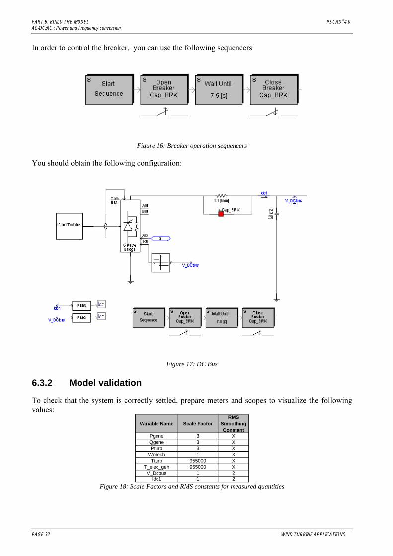
In order to control the breaker, you can use the following sequencers

Figure 16: Breaker operation sequencers

You should obtain the following configuration:

Figure 17: DC Bus

6.3.2 Model validation

To check that the system is correctly settled, prepare meters and scopes to visualize the following values:

Variable Name Scale FactorRMS

Smoothing Constant

Pgene 3 XQgene 3 XPturb 3 X

Wmech 1 XTturb 955000 X

T_elec_gen 955000 XV_Dcbus 1 2

Idc1 1 2 Figure 18: Scale Factors and RMS constants for measured quantities



Simulation parameters: • Duration: 60s • Time step: 100µs • Plot step: 1000µs

Figure 19: Curves obtained with “turb_gen_DC_Connection.psc” The motor torque is always higher than the resistive torque so that the speed increases.As speed increases, Cp decreases so that the turbine power and the turbine torque decreases. At t=7.5s, the resistance is shunted, the capacitor is charged, the over-voltage regulation limits the bus voltage at 1760 V and Idc goes to 0 so that the delivered output power of the generator becomes 0. When Tturb – 0 = f * w; a new steady state is reached.



6.4 6-Pulse Thyristor inverter

6.4.1 Presentation

In this study, the modeled inverter is a current inverter with thyristors (monodirectional in current, bi-directional in voltage). An inductor is added in order to model a current source at the input of the inverter. • Inductor: The energy in the DC bus must be enough to bear a voltage sag of 1 second W = 3 000 000 J. The energy stored in a self-inductor is W = ½ * L *Idc2 Because Idc = Pdc/Vdv = 3*1e6/1600 = 1875 A L = 2*E / Idc2 = 2*3000000 / 18752 = 1.7 H Select an inductor and paste it your model. • Inverter: As for the rectifier, in order to obtain a thyristor current inverter, please select the 6 pulse bridge component. Characterize it as shown in the following figure:

Figure 20: Thyristor Inverter characteristics



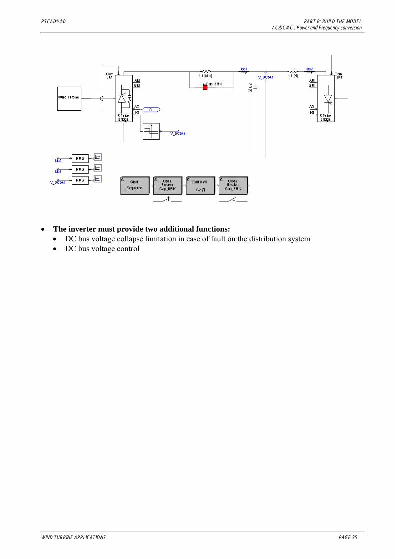
• The inverter must provide two additional functions:

• DC bus voltage collapse limitation in case of fault on the distribution system • DC bus voltage control



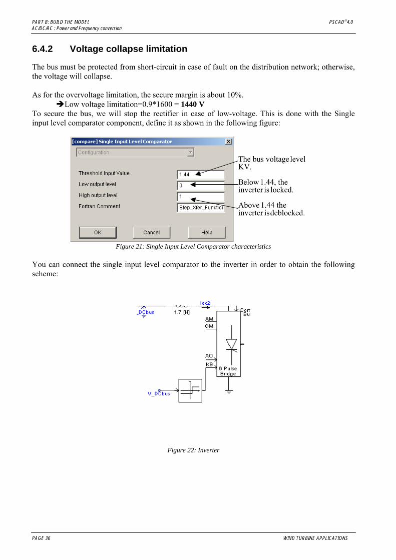
6.4.2 Voltage collapse limitation

The bus must be protected from short-circuit in case of fault on the distribution network; otherwise, the voltage will collapse. As for the overvoltage limitation, the secure margin is about 10%.

Low voltage limitation=0.9*1600 = 1440 V To secure the bus, we will stop the rectifier in case of low-voltage. This is done with the Single input level comparator component, define it as shown in the following figure:

The bus voltagelevelKV.

Below 1.44, theinverter is locked.

Above 1.44 theinverter isdeblocked.

Figure 21: Single Input Level Comparator characteristics

You can connect the single input level comparator to the inverter in order to obtain the following scheme:

Figure 22: Inverter



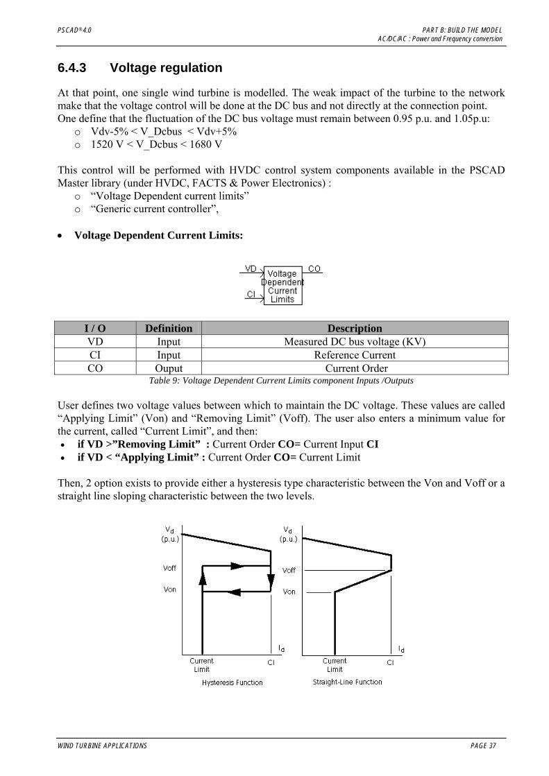
6.4.3 Voltage regulation

At that point, one single wind turbine is modelled. The weak impact of the turbine to the network make that the voltage control will be done at the DC bus and not directly at the connection point. One define that the fluctuation of the DC bus voltage must remain between 0.95 p.u. and 1.05p.u:

o Vdv-5% < V_Dcbus < Vdv+5% o 1520 V < V_Dcbus < 1680 V

This control will be performed with HVDC control system components available in the PSCAD Master library (under HVDC, FACTS & Power Electronics) :

o “Voltage Dependent current limits” o “Generic current controller”,

• Voltage Dependent Current Limits:

I / O Definition Description VD Input Measured DC bus voltage (KV) CI Input Reference Current CO Ouput Current Order

Table 9: Voltage Dependent Current Limits component Inputs /Outputs User defines two voltage values between which to maintain the DC voltage. These values are called “Applying Limit” (Von) and “Removing Limit” (Voff). The user also enters a minimum value for the current, called “Current Limit”, and then: • if VD >”Removing Limit” : Current Order CO= Current Input CI • if VD < “Applying Limit” : Current Order CO= Current Limit

Then, 2 option exists to provide either a hysteresis type characteristic between the Von and Voff or a straight line sloping characteristic between the two levels.



Please configure this component as shown in the following figures:

Note: For the measured voltage, 1 p.u. = 1000V

Below this limit, the current is 0.06 p.u. Above this limit, thecurrent is 1.88 p.u. The minimum currentin the inverter.

Figure 23: Voltage Dependent Current Limits characteristics

The Current Input is the current for the rated power: Idc = Pdc/V_DCbus = 3000000/1600 =1880 A = 1.88 KA

• Generic Current controller:

CO DGE

CD DAPOLPI5GenericCurrentControl

Idc2

I / O Definition Description CD Input Measured DC bus current (KA) CO Input Current order from the “Voltage Dependent Current Limits”

component DA Output The firing angle for the thyristors of the inverter

Table 10: Generic current control Input /Output



The model allows to produce an alpha order from a proportional-integral controller, acting from the error between current order (CO) coming from “Voltage Dependent Current Limits” and measured current (CD) on the DC bus. Configure this component as shown in the following figure:

DC current margin (CM) (+ for inverter,0 or - for rectifier)

Current controller integral gain 3<GI<6 is suggested

Current controller proportional gain (GP). 0.01<GP< 0.02 is suggested [p.u.]

Figure 24: Generic Current Controller characteristics

The entire system should resemble the following figure:

Figure 25: complete_model.psc

Note: Pay attention to the fact that the common potential of the rectifier/inverter/Capacitor is no longer connected to the ground. If it is, this can lead to instability.



6.5 Connection to the network Place the following elements in your system:

Figure 26: Connection between the distributed generator & the distribution network

• Capacitors: Capacitors are added at the output to smooth output voltages and compensate for output reactive power. The simulation allows us to dimension the capacitor: With C=2 mf per capacitor, the reactive power injected to the grid is null. • Transformer: In order to connect the inverter output to the grid a transformer is necessary to adapt the voltage level. Voltage level at the output of the inverter: The current is Ieff-fond = Idc*√6 /π We consider that there are no losses in the inverter: P = 3*V*Ieff-fond cosϕ = Vdv*Idc⇔3*V*Idc*cosϕ*√6 /π = Vdv*Idc⇒V= π*Vdv/(3*√6*cosϕ) The currents in the thyristor must be ahead of the voltage, so in order to have a secure margin, we choose ϕ = π/4: V = 968 V and U = 1675V



Figure 27: Grid Connection transformer characteristics

The complete model should look like the following diagram:

Figure 28: complete_model.psc


PSCAD® 4.0 PART B: BUILD THE MODEL The distribution grid

7. The distribution grid

A distribution grid is a radial grid managed as an open loop. The power always flows in the same direction. Create a new problem: “distribution_grid.psc”.

7.1.1 Definition of the grid

The grid used in this study is shown below:

Figure 29: Distribution grid


PART B: BUILD THE MODEL PSCAD®4.0 The distribution grid

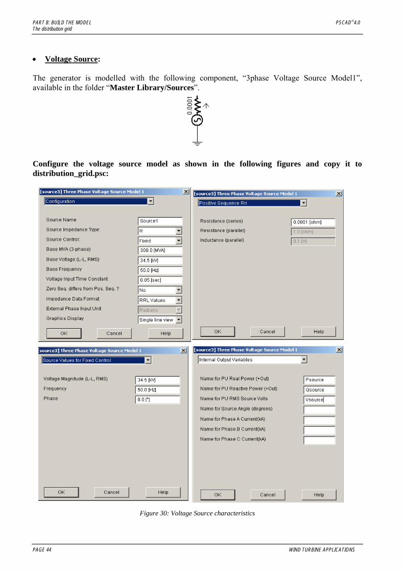
• Voltage Source: The generator is modelled with the following component, “3phase Voltage Source Model1”, available in the folder “Master Library/Sources”.

Configure the voltage source model as shown in the following figures and copy it to distribution_grid.psc:

Figure 30: Voltage Source characteristics



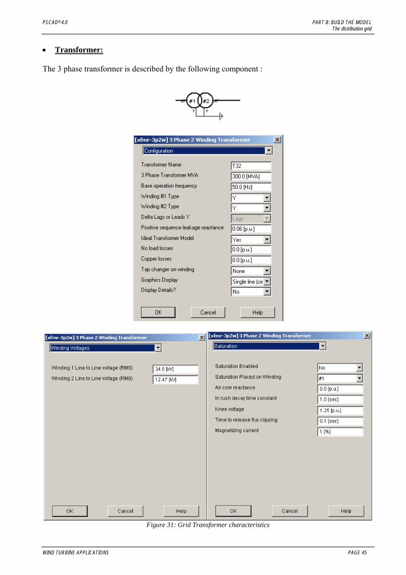
• Transformer: The 3 phase transformer is described by the following component :

Figure 31: Grid Transformer characteristics



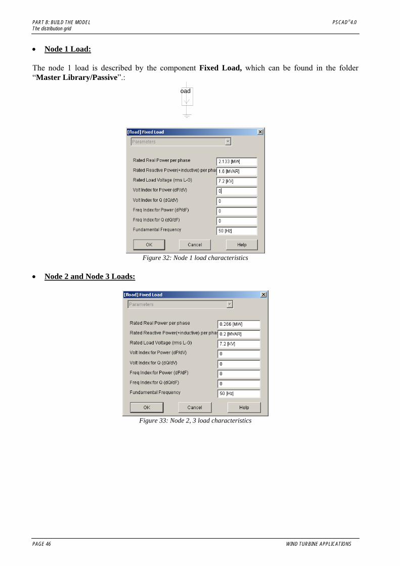
• Node 1 Load: The node 1 load is described by the component Fixed Load, which can be found in the folder “Master Library/Passive”.:

oad

Figure 32: Node 1 load characteristics

• Node 2 and Node 3 Loads:

Figure 33: Node 2, 3 load characteristics



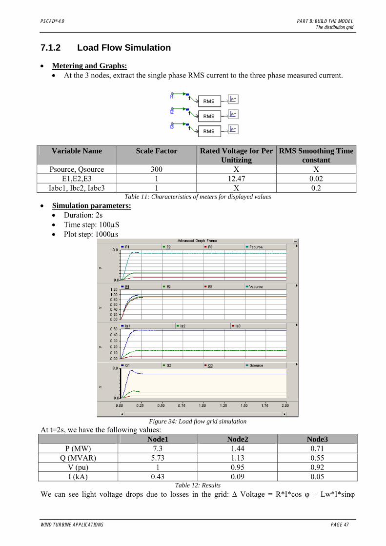
7.1.2 Load Flow Simulation

• Metering and Graphs: • At the 3 nodes, extract the single phase RMS current to the three phase measured current.

Variable Name Scale Factor Rated Voltage for Per

Unitizing RMS Smoothing Time

constant Psource, Qsource 300 X X

E1,E2,E3 1 12.47 0.02 Iabc1, Ibc2, Iabc3 1 X 0.2

Table 11: Characteristics of meters for displayed values • Simulation parameters:

• Duration: 2s • Time step: 100µS • Plot step: 1000µs

Figure 34: Load flow grid simulation

At t=2s, we have the following values: Node1 Node2 Node3

P (MW) 7.3 1.44 0.71 Q (MVAR) 5.73 1.13 0.55

V (pu) 1 0.95 0.92 I (kA) 0.43 0.09 0.05

Table 12: Results We can see light voltage drops due to losses in the grid: ∆ Voltage = R*I*cos ϕ + Lw*I*sinϕ


PSCAD® 4.0 PART C: SIMULATE The distribution grid

PART C: SIMULATE


PART C: SIMULATE PSCAD®4.0 The distribution grid


PSCAD® 4.0 PART C: SIMULATE Constant Wind Study

8. Constant Wind Study

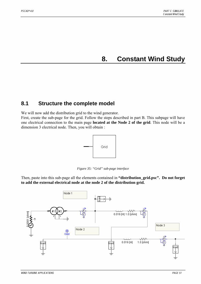
8.1 Structure the complete model We will now add the distribution grid to the wind generator. First, create the sub-page for the grid. Follow the steps described in part B. This subpage will have one electrical connection to the main page located at the Node 2 of the grid. This node will be a dimension 3 electrical node. Then, you will obtain :

Figure 35: “Grid” sub-page interface Then, paste into this sub-page all the elements contained in “distribution_grid.psc”. Do not forget to add the external electrical node at the node 2 of the distribution grid.


PART C: SIMULATE PSCAD®4.0 Constant Wind Study

You will obtain the complete model:

Figure 36: Complete model


PSCAD® 4.0 PART C: SIMULATE Constant Wind Study

8.2 Constant wind study The first study is done with a constant wind speed. Then add meters and channels in order to visualize the following values: Alpha, Idc, Idc2, Pgrid, Qgrid, V_DCbus. • Simulation parameters:

• Duration: 40 s • Time step: 100µs • Plot step: 1000µs • Startup Method: Standard

The results are the following :

Figure 37: constant_wind_study results

• Analysis: The generator voltage increases according to the speed. When Vdv reaches 1440 V, the DC bus regulation is activated and the alpha drive maintains the voltage between 1520V and 1680 V. Once Vdv reaches 1520V, the inverter is unlocked, and Idc2 flows from the DC-bus to the grid.The alpha angle varies according to the measured voltage. We measure 1.6MW for the output active power and no reactive power owing to the capacitors


PART C: SIMULATE PSCAD®4.0 Constant Wind Study


PSCAD® 4.0 PART C: SIMULATE Fault Analysis

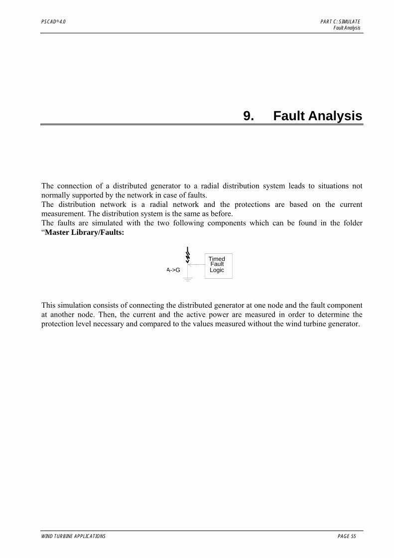
9. Fault Analysis

The connection of a distributed generator to a radial distribution system leads to situations not normally supported by the network in case of faults. The distribution network is a radial network and the protections are based on the current measurement. The distribution system is the same as before. The faults are simulated with the two following components which can be found in the folder “Master Library/Faults:

A->G

TimedFaultLogic

This simulation consists of connecting the distributed generator at one node and the fault component at another node. Then, the current and the active power are measured in order to determine the protection level necessary and compared to the values measured without the wind turbine generator.


PART C: SIMULATE PSCAD®4.0 Fault Analysis

9.1 Default at Node 3

9.1.1 Without DG

First perform a simulation with the distribution grid alone. Add the 3phase fault defined below and connect it at node 3 of the network:

Figure 38: 3Phase fault on the grid

Configure the fault as shown below:

Figure 39: Three phase Fault component characteristics

• Configuration for the Time fault logic component:



Figure 40: Time fault logic configuration

• Simulation parameters:

• Duration: 20 s • Time step: 50 µs • Plot step: 1000 µs

9.1.2 With DG connected at node 1

From the constant wind case, add a fault on the Node 3 of the grid. Set the Wind generator connection to the node 1 of the grid

Figure 41: Timed Fault logic characteristics

Modify the connection between the grid and the distributed generator; in this simulation, the external node will be Node 1.



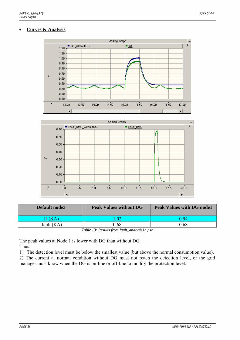
• Curves & Analysis

Default node3

Peak Values without DG Peak Values with DG node1

I1 (KA) 1.02 0.94 Ifault (KA) 0.68 0.68

Table 13: Results from fault_analysis1b.psc The peak values at Node 1 is lower with DG than without DG. Thus: 1) The detection level must be below the smallest value (but above the normal consumption value). 2) The current at normal condition without DG must not reach the detection level, or the grid manager must know when the DG is on-line or off-line to modify the protection level.



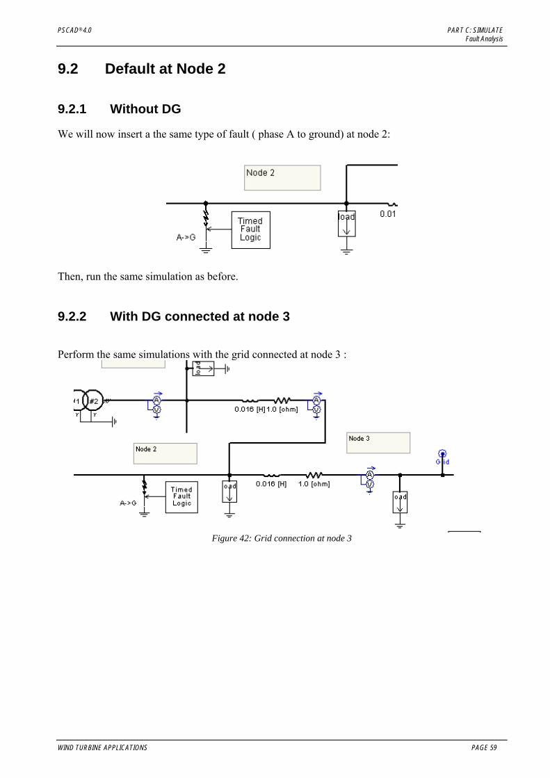
9.2 Default at Node 2

9.2.1 Without DG

We will now insert a the same type of fault ( phase A to ground) at node 2:

Then, run the same simulation as before.

9.2.2 With DG connected at node 3

Perform the same simulations with the grid connected at node 3 :

Figure 42: Grid connection at node 3



• Curves & Analysis:

Figure 43:Current in phase A at node3

Figure 44:Active Power at node 3

Figure 45:Fault current



Default node2 – DG node3 Peak Values without DG Peak Values with DG node3

I3 (KA) 0.02 -0.08 Ifault (KA) 1.43 1.43

Table 14: Simulation results from fault_analysis 2b.psc During a fault, the current at I3 flows in the other direction with DG (the active power is negative). If there is a power protection at this point, this protection will see a negative active power and thus, it will never act! The distributed generator fault current will never be stopped. The peak value at I3 is greater with DG. This could cause a serious problem if the new and larger I3 exceeds the circuit breaker maximum interrupting rating. In this case the circuit breaker must be changed.

9.3 Conclusion The connection of a wind turbine cannot be done directly. The distribution grid is a radial grid and the connection of a distributed generator can modify many uses and controls. Therefore, a complete study must be done because the implementation of a distributed generator will change the protections and circuit breakers needed.


PSCAD® 4.0 PART C: SIMULATE Variable wind study

10. Variable wind study

In this study, two regulations are analysed: • Dynamic pitch control • Passive pitch control

10.1 Dynamic pitch control In this case, β is regulated with the wind turbine governor. In this configuration, the simulation scheme would be:

TmVw

Beta

W P



Wm

Beta

PgMOD 2 Type

Vw

Wind SourceMean

Figure 46: PSCAD model in dynamic pitch control configuration

In this case, the hard-limiter models the cut-in and cut-off values for the wind speed.


PART C: SIMULATE PSCAD®4.0 Variable wind study

Figure 47: Hard limiter in Dynamic pitch control configuration

We will generate the following wind waveform thanks to the CSMF components:

Figure 48: Wind source in variable wind speed study At the beginning, the wind speed is constant at 13m/s to reach the steady state. After t=29s, the wind speed becomes variable thanks to the “Single input level comparator” component with the following parameters :



Figure 49: Single input level comparator settings

Add two breaker operations with sequencers in order to limit the peak current when the wind will reach 13m/s for the second time:

Figure 50: Add two breaker operations to limit current peak at 2nd capacitance charging



Main Simulation parameters: • Duration: 250 s • Time step: 100 µs • Plot Step : 10 000µs

Curves and Analysis:

Figure 51: dyn_pitch.psc results

The beta regulation is aimed at limiting the turbine power at the rated values. We can see that when the turbine power becomes higher than 3.6MW, beta increases, Cp decreases and the output power decreases. The DC bus regulation is still activated when Vdv reaches 1440 V and then, power is delivered to the grid and Alpha varies according to the measured voltage. When the wind decreases, beta decreases in order to increase the input mechanical power, but when the wind decreases too much, Vdv becomes lower than 1440V and the inverter is locked. At the end of the simulation, the turbine power turns negative; this means that the wind turbine is driven by the inertia of the synchronous generator .



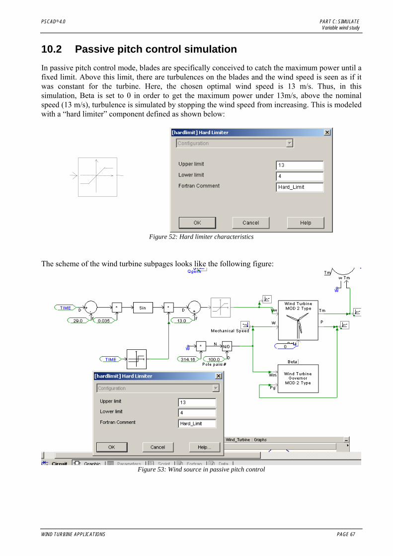
10.2 Passive pitch control simulation In passive pitch control mode, blades are specifically conceived to catch the maximum power until a fixed limit. Above this limit, there are turbulences on the blades and the wind speed is seen as if it was constant for the turbine. Here, the chosen optimal wind speed is 13 m/s. Thus, in this simulation, Beta is set to 0 in order to get the maximum power under 13m/s, above the nominal speed (13 m/s), turbulence is simulated by stopping the wind speed from increasing. This is modeled with a “hard limiter” component defined as shown below:

Figure 52: Hard limiter characteristics

The scheme of the wind turbine subpages looks like the following figure:

Figure 53: Wind source in passive pitch control



• Simulation parameters: • Duration: 250 s • Time step: 100 µs

Plot Step : 10 000µ• s C• urves and Analysis:

Figure 54: passive_pitch.psc results

The wind is modelled with a sinusoidal function between the limits of 4m/s and 13m/s. Compared with the previous simulation, we can observe that the beta regulation does not act, thus, the turbine power coefficient is only a wind speed and a hub speed function.



10.3 Comparison of passive and dynamic pitch control You can see a comparison of power produced by the same wind turbine generator in passive pitch control mode and dynamic pitch control mode. You can directly perform such comparison in “Livewire”:

Figure 55: Comparison between pitch control modes

On these curves, it is easy to see that the pitch regulation tries to maintain the turbine power at its rated value ( 3.6MW) whereas, without dynamic pitch control, the turbine power is not optimized for an entire range of wind speed. Therefore, the energy received in the grid is much larger in dynamic pitch control mode. A wind turbine with dynamic pitch control is more expensive than a passive pitch control, but each time the wind speed is above its rated value, you can get more energy. These simulations would be a reliable basis for the technical-economic study concerning the choice of the pitch control mode.


PSCAD® 4.0 PART C: SIMULATE Wind farm

11. Wind farm

Previously, we simulated a single 3MVA wind turbine. Now we will connect an entire wind farm composed of 100 wind turbines representing a power of 300 MVA, which equals the rated power of the main source of the distribution grid. With connection to the grid power, the output power can no longer be neglected. Therefore, two conditions must be respected at the connection point in order not to cause the grid to become unstable:

• the voltage must be 1 p.u. The voltage regulation must be directly inserted at the connection point.

• the frequency of the inverter must be locked on the grid frequency. In general, a Phase Lock Loop (PLL) is used.


PART C: SIMULATE PSCAD®4.0 Wind farm

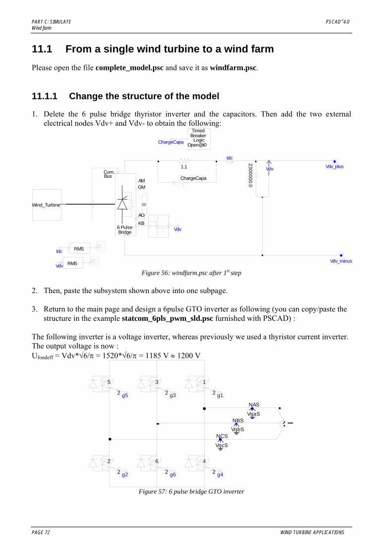
11.1 From a single wind turbine to a wind farm Please open the file complete_model.psc and save it as windfarm.psc.

11.1.1 Change the structure of the model

1. Delete the 6 pulse bridge thyristor inverter and the capacitors. Then add the two external electrical nodes Vdv+ and Vdv- to obtain the following:

KBAO

GMAM

Com.Bus

Bridge6 Pulse Vdv

0

ChargeCapa

TimedBreaker

LogicOpen@t0

1.1

ChargeCapa2300000.0

Idc

Wind_Turbine

Vdv

Vdv_minus

Vdv_plus

Idc

Vdv RMS

RMS

Figure 56: windfarm.psc after 1st step

2. Then, paste the subsystem shown above into one subpage. 3. Return to the main page and design a 6pulse GTO inverter as following (you can copy/paste the

structure in the example statcom_6pls_pwm_sld.psc furnished with PSCAD) : The following inverter is a voltage inverter, whereas previously we used a thyristor current inverter. The output voltage is now : Ufondeff = Vdv*√6/π = 1520*√6/π = 1185 V ≈ 1200 V

VnaS

NAS

VnbS

NBS

VncS

NCS

g1

g2

g3

g4

g5

g6

1

2

3

2

5

2

4

2

6

2

2

2

Figure 57: 6 pulse bridge GTO inverter



4. Connect the different elements, the voltage meters and add the capacitor for the reactive power compensation at the secondary side of the transformer. Finally, you should obtain the following schematics:

Iabc#1 #2

Pow

erAB

PQ

G1 + sT

G1 + sT PgridQgrid

GridWindfarm VnaS

NAS

VnbS

NBS

VncS

NCS

g1

g2

g3

g4

g5

g6

1

2

3

2

5

2

4

2

6

2

2

2

45.0

Vn

3 PhaseRMS Vpu

V_DCbus

V_DCbus

Figure 58: Global view of windfarm.psc

For Vpu RMS measurement: • Voltage per unit: 12.47kV • RMS smoothing Time constant: 2s

11.1.2 Modifications in the synchronous generator

With PSCAD, it is very easy to change a single machine into a “multiple machine” equivalent to several identical machines connected in parallel. It requires only a few changes in the generator’s parameterization: • In the “configuration” window: Choose: “Machine scaling factor : Yes” • In the “basic data”, choose “Number of coherent machines: 100”

Figure 59: Synchronous generator characteristics



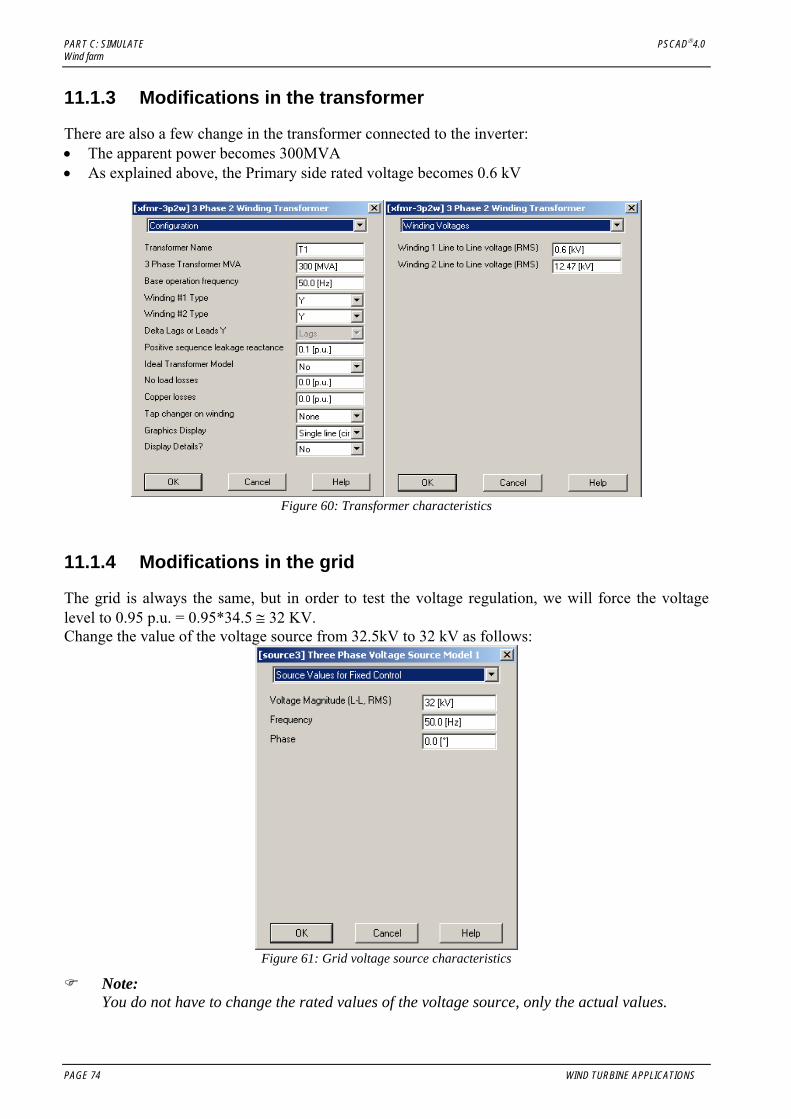
11.1.3 Modifications in the transformer

There are also a few change in the transformer connected to the inverter: • The apparent power becomes 300MVA • As explained above, the Primary side rated voltage becomes 0.6 kV

Figure 60: Transformer characteristics

11.1.4 Modifications in the grid

The grid is always the same, but in order to test the voltage regulation, we will force the voltage level to 0.95 p.u. = 0.95*34.5 ≅ 32 KV. Change the value of the voltage source from 32.5kV to 32 kV as follows:

Figure 61: Grid voltage source characteristics

Note: You do not have to change the rated values of the voltage source, only the actual values.



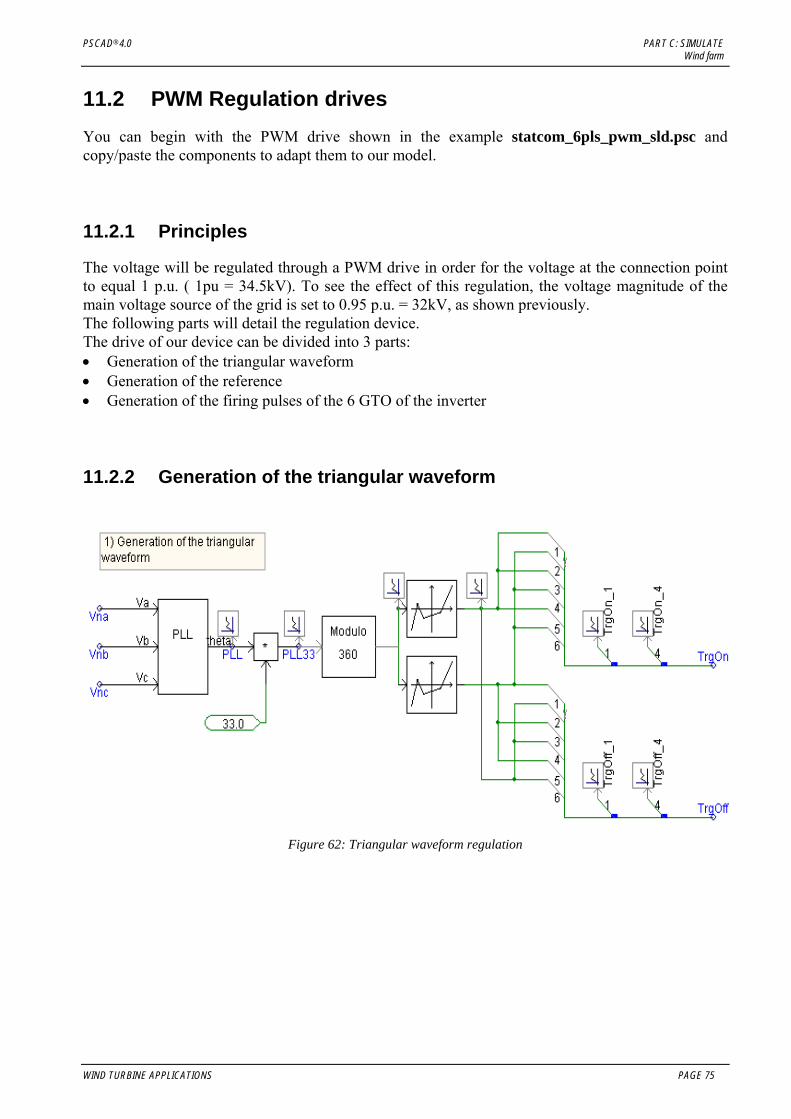
11.2 PWM Regulation drives You can begin with the PWM drive shown in the example statcom_6pls_pwm_sld.psc and copy/paste the components to adapt them to our model.

11.2.1 Principles

The voltage will be regulated through a PWM drive in order for the voltage at the connection point to equal 1 p.u. ( 1pu = 34.5kV). To see the effect of this regulation, the voltage magnitude of the main voltage source of the grid is set to 0.95 p.u. = 32kV, as shown previously. The following parts will detail the regulation device. The drive of our device can be divided into 3 parts: • Generation of the triangular waveform • Generation of the reference • Generation of the firing pulses of the 6 GTO of the inverter

11.2.2 Generation of the triangular waveform

Figure 62: Triangular waveform regulation



This part of the drive system is composed of: • A Phase Locked Loop ( PLL), available in the master library folder “CSMF” and

parameterized as shown below:

Figure 63: PLL characteristics

• 2 non linear transfer characteristic components available in the master library folder “CSMF” and parameterized as shown below: • Generation of the TrgOn signal:

Figure 64: 1st Non linear transfer function characteristics

• Generation of the TrgOff signal:

Figure 65: 2nd Non linear transfer function characteristics



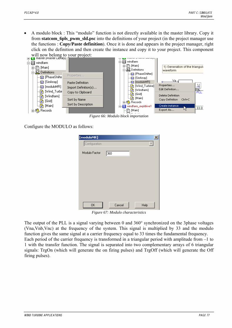
• A modulo block : This “modulo” function is not directly available in the master library. Copy it

from statcom_6pls_pwm_sld.psc into the definitions of your project (in the project manager use the functions : Copy/Paste definition). Once it is done and appears in the project manager, right click on the definition and then create the instance and copy it to your project. This component will now belong to your project:

Figure 66: Modulo block importation

Configure the MODULO as follows:

Figure 67: Modulo characteristics

The output of the PLL is a signal varying between 0 and 360° synchronized on the 3phase voltages (Vna,Vnb,Vnc) at the frequency of the system. This signal is multiplied by 33 and the modulo function gives the same signal at a carrier frequency equal to 33 times the fundamental frequency. Each period of the carrier frequency is transformed in a triangular period with amplitude from –1 to 1 with the transfer function. The signal is separated into two complementary arrays of 6 triangular signals: TrgOn (which will generate the on firing pulses) and TrgOff (which will generate the Off firing pulses).



Advanced Graph Frame

0.130 0.140 0.150 0.160 0.170 0.180 0.190 0.200 0.210 0.220 ...

0

50

100

150

200

250

300

350

400

y

PLL

0.0

2.0k

4.0k

6.0k

8.0k

10.0k

12.0k

y

PLL33

0

50

100

150

200

250

300

350

400

y

Modulo

Figure 68: PLL output


0.2215 0.2220 0.2225 0.2230 0.2235 0.2240 0.2245 0.2250 0.2255 0.2260 ...

-1.00

-0.75

-0.50

-0.25

0.00

0.25

0.50

0.75

1.00

y

nonlinear

-1.00

-0.75

-0.50

-0.25

0.00

0.25

0.50

0.75

1.00

y

TrgOn_1 TrgOn_4

Figure 69: Generated triangular waveform



11.2.3 Generation of the reference

Qgrid

D +

F

-

I

P

TconstPgain

AngleOrder

N

D

N/D

300.0

Shft

N

D

N/D *0.03

TIME *

VpuMaxD

E0.1

D +

F+

Vre

f

Ver

r

Vpu_filter

*40G1 + sT1

1 + sT2

2) Generation of the reference

Va

Vb

Vc

PLLSix

Pulse 6thetaY

Vnc

Vnb

Vna

Sin

Array6 6 1

RefSgnO

n_1

4

45

61

23

123456 Sin

Array6 6 1 4Shft

Shift:

66(in-sh)in

sh

RSgnOn

RSgnOff

RefSgnO

n_4

RefS

gnOff_1

RefS

gnOff_4

Figure 70: Reference signal generation



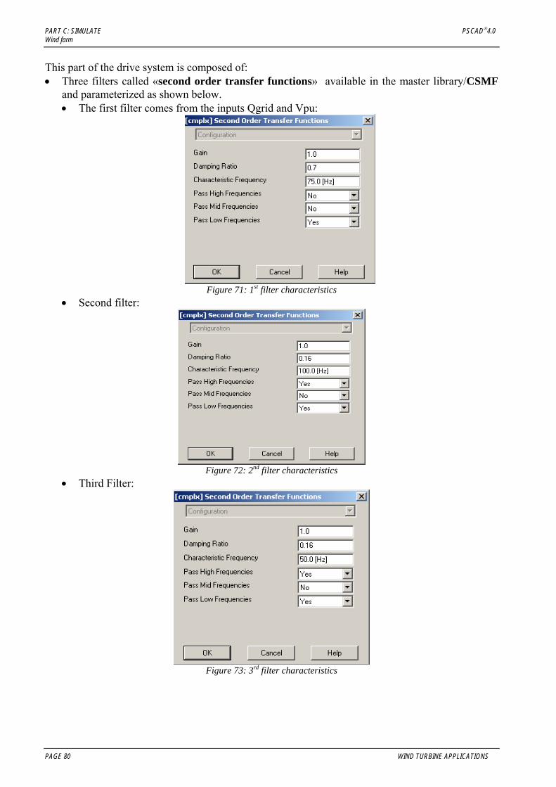
This part of the drive system is composed of: • Three filters called «second order transfer functions» available in the master library/CSMF

and parameterized as shown below. • The first filter comes from the inputs Qgrid and Vpu:

Figure 71: 1st filter characteristics

• Second filter:

Figure 72: 2nd filter characteristics

• Third Filter:

Figure 73: 3rd filter characteristics



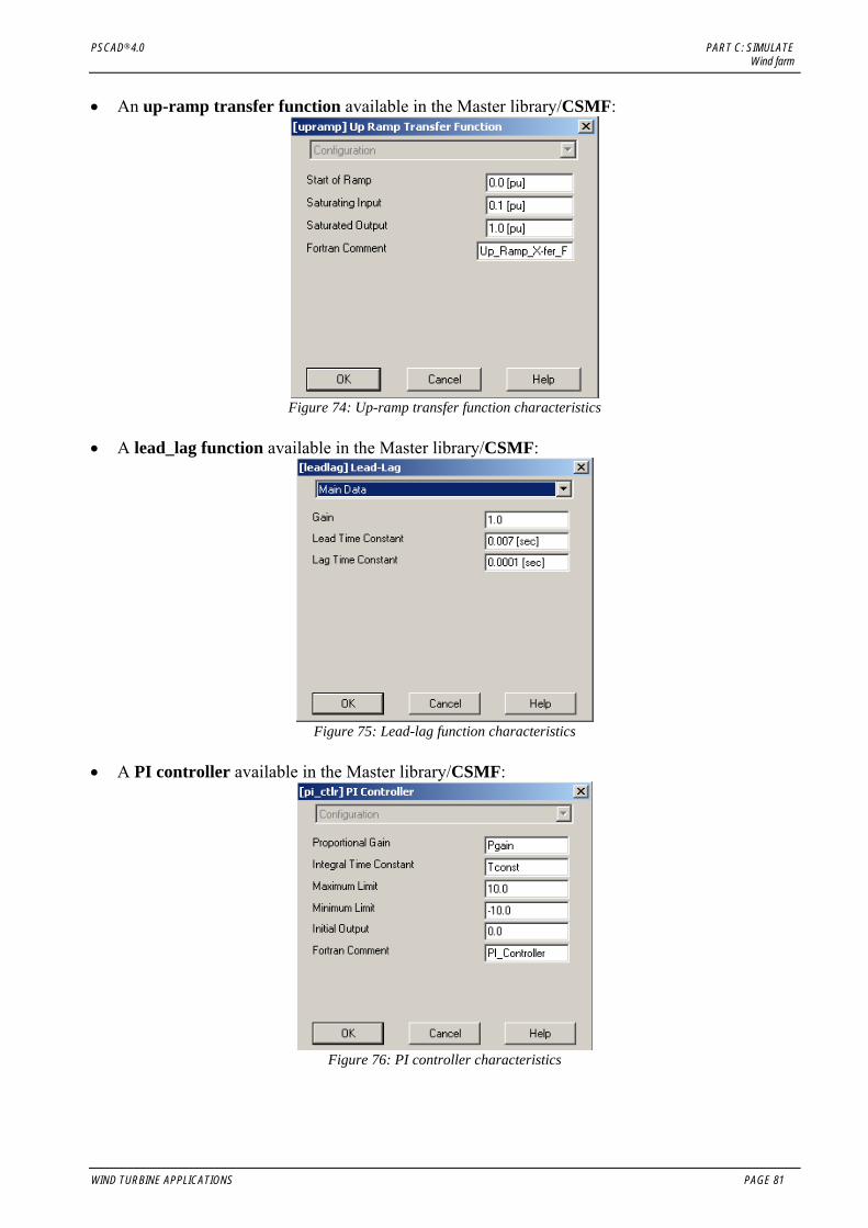
• An up-ramp transfer function available in the Master library/CSMF:

Figure 74: Up-ramp transfer function characteristics

• A lead_lag function available in the Master library/CSMF:

Figure 75: Lead-lag function characteristics

• A PI controller available in the Master library/CSMF:

Figure 76: PI controller characteristics



The gain and the Time constant of the Pi controller and the level of the voltage reference will be controlled with the sliders shown above. • A Phase-Locked Loop six pulse available in the Master library/CSMF:

Figure 77: PLL characteristics

• A component called «Phase_shifter» which you can copy from the example

statcom_6pls_pwm_sld.psc. As for the “modulo” component, you will have to copy/paste the definition and create the instance from the project manager.

• A component called «Sin_array» which you can copy from the example statcom_6pls_pwm_sld.psc. (You will have to copy/paste the definition and create the instance from the project manager).

An error signal Shift is produced from the reference order of the voltage at the connection in Per unit and the measured 3phase RMS voltage at the connection point. Then, this error is subtracted from the six outputs of the PLL, which are 6 signals synchronized on the measured output voltage of the inverter with a 60° phase difference between each one. These signals are organized in order to fit with the GTO arrangement on the bridge and we obtain the reference signals : • RsgnOn for the ON firing pulse • RsgnOff for the Off firing pulse.



Vna_1 is one of the output of the PLL.

Vna_1Shift is Vna_1subtracted with the angleorder (wich is a function of the error betweenthe reference voltage reference and the realvalue).

RefSgnOn_1 is the sinus of Vna_Shift, this isthe reference.

Figure 78: Reference signal generated

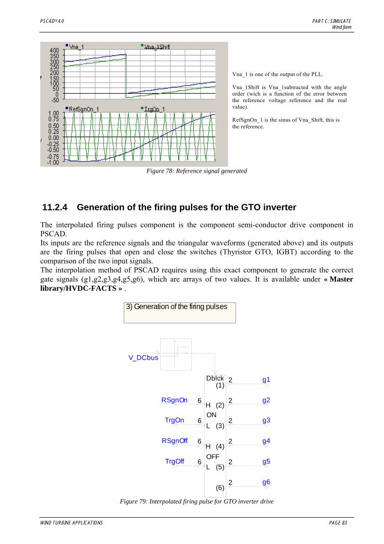
11.2.4 Generation of the firing pulses for the GTO inverter

The interpolated firing pulses component is the component semi-conductor drive component in PSCAD. Its inputs are the reference signals and the triangular waveforms (generated above) and its outputs are the firing pulses that open and close the switches (Thyristor GTO, IGBT) according to the comparison of the two input signals. The interpolation method of PSCAD requires using this exact component to generate the correct gate signals (g1,g2,g3,g4,g5,g6), which are arrays of two values. It is available under « Master library/HVDC-FACTS » .

g1

g4

g6

g3

g2

g5

Dblck

6

6

6

6

L

H

HON

OFFL

(1)

(4)

(5)

(6)

2

2

2

(2)

(3)

2

2

2

TrgOn

TrgOff

RSgnOn

RSgnOff

V_DCbus

3) Generation of the firing pulses

Figure 79: Interpolated firing pulse for GTO inverter drive



The measure of the voltage V_DCbus blocks and unblock the signals. Please configure this component as follows:

Figure 80: Interpolated Firing pulse characteristics

The input and output signals look like the following:

Figure 81: Gate signals generated



11.3 Simulation • Simulation parameters:

• Duration: 70 s • Time step: 100 µs • Plot step: 2000 µs • Startup method: Standard

Variable Name Scale Factor Rated Voltage for Per

Unitizing RMS Smoothing Time

constant Psource, Qsource 300 X 2

P2,Q2 1 X 2 P4,Q4 1 X 2

Vsource 1 X 2 Vconnection 1 12.47 2

Table 15: Metering characteristics for measured quantities • Curves and Analysis:

1 1 Advanced Graph Frame

0 10 20 30 40 50 60 70 ... ......

0.00 0.20 0.40 0.60 0.80 1.00 1.20 1.40 1.60

y

Vdv


0 10 20 30 40 50 60 70 ... ......

-4.0 -2.0 0.0 2.0 4.0 6.0 8.0 10.0 12.0 14.0

y

P2 P4 Psource

Figure 82: Windfarm.psc results




0 10 20 30 40 50 60 70 ...

-3.0 -2.0 -1.0 0.0 1.0 2.0 3.0 4.0 5.0 6.0 7.0

yQ2 Q4 Qsource

3 3 3


0 10 20 30 40 50 60 70 ... ... ...

0.00 0.20 0.40 0.60 0.80 1.00 1.20

y

Vsource V_connection(pu)

Figure 83: Windfarm.psc results

At t = 5s the resistance is shunted, thus the voltage drops. When Vdv reaches 1520V, the regulation starts. Before the starting of the regulation, the connection point voltage ( V4) is imposed by the grid. Afterward, the regulation set it to 1pu The wind farm produces 3.5 MW to maintain the voltage at 1pu (P4).


PSCAD® 4.0 PART D: APPENDIX

PART D: APPENDIX


PART D: APPENDIX PSCAD®4.0


PSCAD® 4.0 PART D: APPENDIX References

12. References

• IEEE articles:

• [1] P.M. Anderson, Anjan Bose, Stability Simulation Of Wind Turbine Systems, Transactions On Power Apparatus And Systems. Vol. PAS 102, No. 12, December 1983, pp. 3791-3795.

• Grid friendly connection of constant speed wind turbines using external resistors: Torbjorn Thiringer; IEEE Transactions on energy conversion Vol 17, N°4; December 2002

• Direct Methods For transient stability assesment in power systems comprising controllable Series Device; Gabrijel/Mihalic; Vol 17, N°4; November 2002

• Improving Voltage Disturbance Rejection for Variable-Speed Wind turbines; Saccomando/Svensson/Sannino; Vol 17, N°3; September 2002

• PSCAD/EMTDC based simulation of a wind-diesel conversion scheme; Kannan Rajendiran; Curtin University of Technology, Perth, Australia; [email protected]; IEEE 2000

• Other articles:

• Modelisation de générateurs éoliens à vitesse variable connectés à un bus continu commun/Modelling of variable speed wind generators jointly connected to continuous bus; El Aimani/François/Robyns (L2EP); FIER 2002; http://www.fst.ac.ma/fier/59.PDF

• Eolienne lente de proximité, conception, performances, technologie et application; slow rotating wind turbine for proximity applications, criteria of design expected performances technology and applications; Bouly/Defois/Faucillon/Billon; FIER 2002; http://www.fst.ac.ma/fier/57.PDF

• Control issues of a permanent magnet generator variable speed wind turbine: Chaniotis/Papathanassiou/Kladas/Papadopoulos (National Technical University of Athens); http://www.cc.ece.ntua.gr/~achan/Kataskeues/MED02-107.pdf

• Manuals:

• Eoliennes et aérogénérateurs. Guide de l’énergie éolienne; Guy Cunty; Edisud


mailto:[email protected]

http://www.fst.ac.ma/fier/59.PDF

http://www.fst.ac.ma/fier/57.PDF

http://www.cc.ece.ntua.gr/~achan/Kataskeues/MED02-107.pdf

PART D: APPENDIX PSCAD® 4.0 References


PSCAD: Power System Simulationforum.hvdc.ca/DownloadFile.aspx?file=UserFiles... · PSCAD® 4.2 PART...

Documents

Transcript of PSCAD: Power System Simulationforum.hvdc.ca/DownloadFile.aspx?file=UserFiles... · PSCAD® 4.2 PART...