
PROYECTO FINAL DE CARRERA Seismic and vibration signal...
129
PROYECTO FINAL DE CARRERA Seismic and vibration signal analysis and monitoring using LabVIEW AUTOR Mariano Martínez DIRECTOR Simon Platt(UCLAN) SUPERVISOR UNIV.ZARAGOZA Antonio Bono ESPECIALIDAD Electrónica CONVOCATORIA Junio 2012 Desarrollado en programa de intercambio en:
Transcript of PROYECTO FINAL DE CARRERA Seismic and vibration signal...

PROYECTO FINAL DE CARRERA
Seismic and vibration signal analysis
and monitoring using LabVIEW AUTOR
Mariano Martínez
DIRECTOR
Simon Platt(UCLAN)
SUPERVISOR UNIV.ZARAGOZA
Antonio Bono
ESPECIALIDAD
Electrónica
CONVOCATORIA
Junio 2012
Desarrollado en programa de
intercambio en:

University of Central Lancashire. School of Computing, Engineering and Physical Sciences
2
School of Computing, Engineering
and Physical Sciences
MARIANO MARTINEZ
SEISMIC AND VIBRATION SIGNAL
ANALYSIS AND MONITORING
USING LabVIEW
(EL3990)
Submitted in partial satisfaction of the
requirements for the degree of
Bachelor of Engineering (with Honours)
in
1. Electronic Engineering
April 2012
I declare that all material contained in
this report, including ideas described in
the text, computer programs and
drawings, is my own work except
where explicitly and individually
acknowledged.
Signed …………………….
Date ……………………….

University of Central Lancashire. School of Computing, Engineering and Physical Sciences
3
Abstract
Every year there are around 20 earthquakes of magnitude 7 or above (PREPA.R.E, 2008).
This kind of seismic events are potentially destructive and can cause several structural
damage, economic and human loss. In order to perform an efficient risk management and
prevention work geophysics must be equipped with suitable software and hardware tools.
Seismic studies comprise not only risk management but earth structure studies that are useful
in gas and oil prospections. Vibration monitoring has also turned in a very useful scientific
approach to deal with structural safety and maintenance. Among these devices, MEMS
accelerometer combines great performance with low costs, characteristics that have made it
one of the most popular devices when it comes to this task. (Santoso, 2010).
Seismic analysis software has been developed using LabVIEW. The software decodes SAC
data files and retrieves important seismic parameters like arrival wave times, location and
magnitude. The precision and performance reached is acceptable for the scope of this project
and it could be used as a domestic seismic analyser but not for its use in a professional
seismic station. The seismic data for the system evaluation was retrieved from IRIS database.
(IRIS, 2011)
A vibration DAQ and monitoring module has been designed and implemented. It successfully
measures and monitors acceleration versus time and the signal’s spectra. Zooming options
were included in order to make easier the background noise and ambient vibration study
(Attri R. K., 2004). An instant and maximum earthquake intensity gauge was programmed to
give an idea of the experienced event potential danger. The user can selectively save
acceleration time responses in LVM format.
An analogue output was implemented. It is capable of reading acceleration versus time
responses saved in LVM and SAC files and output them using a DAQ card analogue output
function. This voltage can be seen in an oscilloscope or input to other devices.
In order to acquire and save the analogue waveforms created with the previous function an
analogue input was included as an initial objective in the Scheme of Work. However, it was
dropped in the final implementation because it was considered that its function was too
similar to the vibration DAQ module and it did not have enough practical application.

University of Central Lancashire. School of Computing, Engineering and Physical Sciences
4
Acknowledgements
I would like to take this opportunity to express my gratitude to all the academic staff that has
helped me during the development of this final project. Particularly to Simon Platt for sharing
his knowledge, the orientation, material lent and the doubts solved. I’d also like to express my
gratitude to David Heys in whose SIC tutorial sessions I sometimes had project related
enquiries. I would like to show my appreciation to the Stores staff for their kindness, good
work and also for the patience showed the busy laboratory days. I wouldn’t like to forget
University of Zaragoza professors, as the knowledge obtained in their lessons were essential
to bring this project into a conclusion. I would like to show my appreciation to the UCLAN
instruction for giving me the opportunity of studying here this year and the budget assigned to
buy the materials I needed for the project execution. Many thanks to the Google team as their
search tool has saved me enormous amounts of time being a key tool during the great amount
of background information I had to research.

University of Central Lancashire. School of Computing, Engineering and Physical Sciences
5
Table of contents Abstract ................................................................................................................................................... 3
Acknowledgements ................................................................................................................................. 4
Table of contents .................................................................................................................................... 5
List of tables ............................................................................................................................................ 7
List of equations ...................................................................................................................................... 7
List of figures ........................................................................................................................................... 8
List of abbreviations .............................................................................................................................. 11
1. Introduction .................................................................................................................................. 12
1.1 Motivation ................................................................................................................................... 12
1.2 Aim and objectives ..................................................................................................................... 13
1.3 Scope ........................................................................................................................................... 14
1.4 Literature review ......................................................................................................................... 15
2. Background ................................................................................................................................... 18
2.1 Vibration Monitoring Instrumentation Systems ......................................................................... 18
2.1.1 Introduction and applications ............................................................................................... 18
2.1.2 Instrumentation Systems for Data Acquisition .................................................................... 18
2.1.3 Vibration transducers ........................................................................................................... 19
2.1.4 Accelerometers..................................................................................................................... 20
2.1.5 Acceleration, intensity and damage ..................................................................................... 20
2.2 Seismological data analysis ........................................................................................................ 22
2.2.1 Introduction to earthquakes and seismic waves ................................................................... 22
2.2.2 Measuring and recording seismic data ................................................................................. 24
2.2.3 Seismic Data ........................................................................................................................ 25
2.3.4 Seismic Data in LabVIEW. SAC format ............................................................................. 25
2.3.5 Earthquake parameters computation overview .................................................................... 26
2.3.6 Processing timing parameters .............................................................................................. 28
2.3.7 Processing location parameters ............................................................................................ 30
2.3.8 Processing magnitude parameters ........................................................................................ 31
3. Vibration Monitoring System Design ............................................................................................ 35
3.1 Hardware ..................................................................................................................................... 35
3.1.1 Accelerometer choice ........................................................................................................... 35
3.1.2 DAQ selection ...................................................................................................................... 37
3.1.3 Data acquisition structure..................................................................................................... 39
3.1.4 Signal conditioning .............................................................................................................. 40

University of Central Lancashire. School of Computing, Engineering and Physical Sciences
6
3.1.5 ADXL203EB Evaluation board ........................................................................................... 43
3.1.6 Enclosure and mounting....................................................................................................... 43
3.1.8 PCB ...................................................................................................................................... 45
3.1.9 EMI/EMC considerations .................................................................................................... 46
3.2 Software ...................................................................................................................................... 47
3.2.1 Global software framework ................................................................................................. 47
3.2.2 DAQ ..................................................................................................................................... 47
3.2.3 Axis calibration .................................................................................................................... 47
3.2.4 Earthquake intensity and danger .......................................................................................... 48
3.2.5 Display characteristics and saving options .......................................................................... 49
4. Seismological data analysis software design ................................................................................ 50
4.1 Introduction and Specifications .................................................................................................. 50
4.2 Data format selection .................................................................................................................. 50
4.3 Global software framework ....................................................................................................... 51
4.4 Reading SAC files ....................................................................................................................... 51
4.5 Frequency analysis and optional filtering ................................................................................... 52
4.6 Arrival times ............................................................................................................................... 52
4.6.1 Introduction .......................................................................................................................... 52
4.6.2 Automatic picking ................................................................................................................ 52
4.6.3 Manual picking .................................................................................................................... 55
4.7 Coda length ................................................................................................................................. 55
4.8 Distance to the epicentre ............................................................................................................. 56
4.9 Magnitude ................................................................................................................................... 58
5. Analogue output design ................................................................................................................ 60
6. Vibration monitoring system construction and implementation ................................................. 61
6.1 Hardware ..................................................................................................................................... 61
6.2 Software ...................................................................................................................................... 62
7. Seismological data analysis software implementation ................................................................. 64
8. Analogue output software implementation ................................................................................. 69
9. Dataflow and Interface ................................................................................................................. 70
10. System evaluation and results .................................................................................................. 72
10.1 Vibration DAQ evaluation ........................................................................................................ 72
10.2 Seismic analysis evaluation ...................................................................................................... 75
10.3 Analogue output evaluation ...................................................................................................... 86
11. Future work: Potential improvements and modifications .............................................................. 87

University of Central Lancashire. School of Computing, Engineering and Physical Sciences
7
12. Conclusion ................................................................................................................................. 89
Appendix A: Detailed Seismic analysis software ................................................................................... 91
Appendix B: Detailed Vibration DAQ software ................................................................................... 106
Appendix C: Detailed analogue output software................................................................................ 110
Appendix D: Brief Instructions for use ............................................................................................... 113
Appendix E : Planning documents ...................................................................................................... 117
Appendix F: DAQ Circuit and PCB plans .............................................................................................. 119
Appendix G: DAQ hardware components list ..................................................................................... 126
List of tables Table 2.1:Mercalli intensity scale relationship with PGA (PREPA.R.E, 2008)........................................ 22
Table 2.2 Seismic data global computation .......................................................................................... 27
Table 2.3: Approximate Magnitude vs Size equivalence ..................................................................... 32
Table 3.1: Input range and resolution for NI 6221 ............................................................................... 38
Table 10.1 Software magnitude calculations evaluation. Comparison with magnitude of different
data retrieved from ISIS. ....................................................................................................................... 78
Table 10.2 Coda magnitude characteristics verification ....................................................................... 79
Table 10.3Threshold determination for different earthquakes ........................................................... 81
Table 10.4: Automatic and manual picking comparrison ..................................................................... 82
Table G.1 DAQ hardware component list ........................................................................................... 126
List of equations Equation 2.1: STA and LTA equations ................................................................................................... 28
Equation 2.2: Distance formulas ........................................................................................................... 31
Equation 2.3: Local magnitude ............................................................................................................. 32
Equation 2.4: Coda/duration magnitude .............................................................................................. 32
Equation 3.1: Anti-aliasing condition ................................................................................................... 38
Equation 3.2: Satisfactory conversion time demonstration ................................................................. 38
Equation 3.3: Cut-off frequency and added capacitors relationship (Analog Devices, 2011) .............. 41
Equation 3.4: Accelerometer noise ....................................................................................................... 41
Equation 4.1: STA/LTA ratio equations ................................................................................................. 52
Equation 4.2:Coda length...................................................................................................................... 56

University of Central Lancashire. School of Computing, Engineering and Physical Sciences
8
List of figures Figure 1.1: Software main structure ..................................................................................................... 13
Figure 1.2: Global software specifications ............................................................................................ 15
Figure 2.1: DAQ general structure ........................................................................................................ 18
Figure 2.2: Earthquake origin. Image by Taiwanese Central Weather Bureau ( Central Weather
Bureau, 2012) ........................................................................................................................................ 23
Figure 2.3: P waves Figure 2.4 S waves .......................................................................................... 24
Figure 2.5: STA LTA algorithm illustration (Han, 2010) ......................................................................... 29
Figure 2.6: Coda length illustration ....................................................................................................... 30
Figure 2.7: Generic depth distance travel time dependence and epicentre plotting (Havskov &
Ottemöller, 2010) ................................................................................................................................. 31
Figure 2.8: Coda Magnitude parameters in different areas of the world (Havskov & Ottemöller, 2010)
.............................................................................................................................................................. 33
Figure 2.9: Magnitude scale conversion table (Havskov & Ottemöller, 2010) ..................................... 34
Figure 3.1: Hardware block diagram .................................................................................................... 39
Figure 3.2: Schematics design ............................................................................................................... 40
Figure 3.3: Connection scheme used .................................................................................................... 42
Figure 3.4: BNC 2120 GS input ........................................................................................................... 42
Figure 3.5: ADXL Evaluation board........................................................................................................ 43
Figure 3.6:1591XXMS Dimensions ........................................................................................................ 44
Figure 3.7:1591XXMS 3D model ......................................................................................................... 44
Figure 3.8:PCB artwork ......................................................................................................................... 45
Figure 3.9: PCB 3D model...................................................................................................................... 46
Figure 3.10: Vibration DAQ software framework ................................................................................. 47
Figure 3.11: Calibration subroutine flowchart ...................................................................................... 48
Figure 3.12: Magnitude and danger calculator subroutine .................................................................. 48
Figure 4.1 Seismic analysis software specifications .............................................................................. 50
Figure 4.2: Global computation framework (Attri R. K., 2005) ............................................................. 51
Figure 4.3: Read data flowchart ............................................................................................................ 51
Figure 4.4: Automatic Arrival time picking global flowchart ................................................................ 53
Figure 4.5: STA/LTA ratio implementation subroutine flowchart ........................................................ 54
Figure 4.6: STA/LTA one sample subroutine flowchart ........................................................................ 55
Figure 4.7: Pick arrival times subroutine .............................................................................................. 55
Figure 4.8: Coda length subroutine algorithm ...................................................................................... 55
Figure 5.1: Analogue output specifications .......................................................................................... 60
Figure 5.2: Analogue output flowchart ................................................................................................. 60
Figure 6.1 Vibration sensor device without the lid and header on which the evaluation board is
mounted ................................................................................................................................................ 61
Figure 6.2: Complete vibration sensor module. ................................................................................... 61
Figure 6.3 code section comprising DAQ assistant and calibration VI .................................................. 62
Figure 6.4: Vibration DAQ front panel .................................................................................................. 62
Figure 6.5: "Intensity and danger Display" VI in the vibration DAQ main code ................................... 63
Figure 7.1Seismic analysis VI front panel .............................................................................................. 64
Figure 7.2Code sections where the mentioned SubVIs are used ......................................................... 65

University of Central Lancashire. School of Computing, Engineering and Physical Sciences
9
Figure 7.3 Seismogram and its spectra ................................................................................................. 65
Figure 7.4 Filtering options in the seismic analysis front panel ............................................................ 66
Figure 7.5 : STA LTA ratio and Pick arrival times VIs in the main seismic code .................................... 66
Figure 7.6 STA/LTA ratio VI front panel. The figure shows an earthquake seismogram, the STA/LTA
ratio and the STA and LTA waves for specific L1 and L2 window lengths ........................................... 67
Figure 7.7 Cursors and controls for manual picking in the seismic analysis VI front panel(left) and the
loop that actualises coda length and S-P when the use modifies arrival times. ................................. 68
Figure 7.8 "Coda length" VI in the main seismic code .......................................................................... 68
Figure 7.9: Distance to the epicentre subVI placed in the seismic analysis code. ................................ 69
Figure 7.10: Magnitude controls and indicators in the front panel ..................................................... 69
Figure 8.1: Analogue output VI front panel .......................................................................................... 70
Figure 9.1: Example of the event structure continuously used in the software. The External loop
keeps it running. The shift registers and local variables can be seen. .................................................. 71
Figure 9.2: Main menu interface .......................................................................................................... 71
Figure 10.1: Hardware system distribution for vibration DAQ and output testing .............................. 72
Figure 10.2: Accelerometer voltage outputs when tilted so that the two axes support different
accelerations ......................................................................................................................................... 72
Figure 10.3: DAQ front panel when running ......................................................................................... 73
Figure 10.4: Light table hitting (Y axis) time and frequency responses ................................................ 73
Figure 10.5: Strong enclosure hitting (X axis) time responses .............................................................. 74
Figure 10.6: Strong shaking time and frequency responses ................................................................. 74
Figure 10.7: Heavy shaking time and frequency responses ................................................................. 75
Figure 10.8 Software distance calculations compared to USGS Distance vs S-P time table ................ 77
Figure 10.9: STA/LTA ratio VI front panel ............................................................................................. 80
Figure 10.10: Averaged threshold ......................................................................................................... 82
Figure 10.11: Coda length calculator problem ..................................................................................... 84
Figure 10.12: Non- filtered seismogram ............................................................................................... 85
Figure 10.13: Seismogram spectra ........................................................................................................ 85
Figure 10.14: Filtered seismogram. Low cut-off = 0. 01 Hz. High cut-off =1 Hz ................................... 85
Figure 10.15: Analogue output front panel running and reading a SAC file. ........................................ 86
Figure 10.16: LVM vibration file reading and analogue output ............................................................ 86
Figure 10.17: SAC file reading and analogue output ........................................................................... 87
Figure A. 1: Seismic analysis VI front panel........................................................................................... 91
Figure A. 2: Seismic analysis VI global structure. Timeout event. ........................................................ 91
Figure A. 3: Seismic analysis VI. Read file event ................................................................................... 92
Figure A.4 Seismic analysis VI. Automatic picking event ...................................................................... 92
Figure A. 5: Seismic analysis VI .Frequency analysis event ................................................................... 93
Figure A. 6:Seismic analysis VI.Filter event ........................................................................................... 93
Figure A.7: Seismic analysis VI. Calculate distance event .................................................................... 94
Figure A.8: Seismic analysis VI. Calculate magnitude event ................................................................. 94
Figure A..9: Seismic analysis VI. Stop event. ......................................................................................... 95
Figure A.10: Read SAC VI icon ............................................................................................................... 96
FigureA.11: Retrieve properties VI block diagram ................................................................................ 97
Figure A.12: STA LTA ratio front panel .................................................................................................. 98
Figure A.13: STA LTA ratio VI Start event and global VI structure ........................................................ 99

University of Central Lancashire. School of Computing, Engineering and Physical Sciences
10
FigureA.14:STA LTA ratio VI BACK event ............................................................................................... 99
FigureA.15: STA LTA one sample VI icon ............................................................................................. 100
Figure A.16:STA LTA one sample block diagram ................................................................................. 100
Figure A.17: Pick arrival times VI icon ................................................................................................. 101
Figure A.18: Pick arrival times VI block diagram ................................................................................. 101
FigureA.19: Frequency analysis VI icon ............................................................................................... 102
FigureA.20: Frequency analysis VI front panel ................................................................................... 102
FigureA.21: Frequency analysis VI block diagram ............................................................................... 103
Figure A.22: Distance to the epicentre icon ....................................................................................... 103
Figure A.23: Distance to the epicentre block diagram ....................................................................... 103
Figure A.24: Distance to the epicentre case structures ...................................................................... 104
Figure A.25 Coda length meter ........................................................................................................... 104
FigureA.26: Coda length meter VI block diagram ............................................................................... 104
Figure A.27: Gather signals below a threshold VI icon ....................................................................... 105
Figure A.28: Gather signals below a threshold block diagram (NI Instructors, 2011) . ...................... 105
Figure B.1: Vibration DAQ VI front panel ............................................................................................ 106
Figure B.2: Vibration DAQ event structure. Timeout. ......................................................................... 106
Figure B.3: Vibration DAQ VI. Acquire event ...................................................................................... 107
FigureB.4: Vibration DAQ VI Main menu event .................................................................................. 107
FigureB.5: Vibration DAQ VI pause event ........................................................................................... 108
FigureB.6: Axes calibration VI icon ...................................................................................................... 108
FigureB.7: Axes calibration VI block diagram ...................................................................................... 108
FigureB.8: Intensity and danger display VI icon .................................................................................. 109
Figure B0.9: Intensity and danger display VI front panel .................................................................... 109
FigureC.1: Analogue output VI front panel ......................................................................................... 110
FigureC.2: Analogue output VI .Timeout event .................................................................................. 110
Figure C.3: Analogue output VI. Read file event. ................................................................................ 111
Figure C.4: Analogue output VI. Start output event. .......................................................................... 112
Figure C. 5: Analogue output VI. Back event ...................................................................................... 112
Figure D.1: Seismic analysis main window instructions ...................................................................... 113
Figure D.2: STA LTA ratio VI front panel instructions ......................................................................... 114
Figure D.3: Vibration DAQ VI instructions .......................................................................................... 115
Figure D.4: Analogue output VI instructions ....................................................................................... 116
Figure D.1: Gantt diagram ................................................................................................................... 117
Figure D.2: Risk register ...................................................................................................................... 118

University of Central Lancashire. School of Computing, Engineering and Physical Sciences
11
List of abbreviations ADC – Analogue to digital conversion
AO – Operational amplifier
BGS – British Geological Survey
BNC – British Naval Connector
COSMOS –The Consortium of Organizations for Strong-Motion Observation Systems
CSMIP – California Strong Motion Instrumentation Program
DAQ – Data acquisition
GSEC – Group of Scientific experts
IEPE – Integral Electronics Piezoelectric
IRIS – Incorporated Research Institutions for seismology
K-NET – Kyoshin Net
LCC – Leadless chip carrier
LTA – Long-time average
LVM - LabVIEW Measurement file
MEMS – Microelectromechanical systems
MMIS – Modified Mercalli Intensity Scale
NIED – National l Research Institute for Earth Science and Disaster Prevention
PCB – Printed circuit board
PGA – Peak Ground Acceleration
SA – Spectra acceleration
SAC – Seismic Analysis Code
SCEDC – The Southern California Earthquake data center
SEED – The Standard for the Exchange of Earthquake Data
SNR – Signal to noise ratio
STA – Short time average
USGS – US geological Survey
VI – Virtual instrument (LabVIEW)

University of Central Lancashire. School of Computing, Engineering and Physical Sciences
12
1. Introduction
1.1 Motivation Last spring, on March 11th of 2011 immediately after the earth shook in Japan there were
alarms throughout their entire east coast warning people to head towards highest places.
Furthermore, the trains and underground of Tokyo actually stopped before the dangerous
surface waves reached the city to prevent derailments. Meanwhile, the passengers were
warned some seconds before the trains started to swing. Most of the buildings that compound
Tokyo’s skyline were swaying instead of collapsing since sooner or later a large earthquake
was expected. These preventing actions were possible thanks to a well-developed science that
is lately making huge steps thanks to the new technologies to detect signals and store, analyse
and monitor data efficiently so that the specialists can work fast and precisely. It is not
necessary to go to Japan to experience earthquakes, here in Britain microseims occur every
year and although hardly perceptible by human, they are used by the experts to study the earth
structure (British Geological Survey, 2012). There are no more tremors now than 100 years
ago. Nevertheless, due to the increasing population in the globe the effects have become
devastating and the human and structural loss unacceptable. Geophysics and structural
engineers need modern tools to face this challenge, and this was the central stimulus to focus
my work on this issue (Attri R. K., 2004). The analysis of seismological events also allows
the geophysics to determine the earth structure; they perform a key role in the detection of
cavities and therefore are essential to obtain data on oil and gas prospection.
The acquisition of seismic data involves complex DAQ systems, proper locations,
infrastructure and expensive sensors like seismometers, geophones or special accelerometers.
(Turk et al, 2011). The monitoring and assessment of the vibrations that affect structures
during an earthquake, other events or just the study of noise level vibration are essential to
save lives, minimize damage as well as to aid with the maintenance of a structure and detect
possible failures. Usually, traditional instrumentation systems to monitor structure and noise
level vibration are complex and expensive. There is an increasing demand of better and
cheaper monitoring systems and the low cost signal-conditioned MEMS accelerometers are
among the devices that possibilities these features in a system. (Wenzel & Pichler, 2005)
(Santoso, 2010)
LabVIEW is a comprehensive graphic programming language and development environment
established by National Instruments which is loved among engineers that can see the flow of
the data rather than text based programming. LabVIEW is industry standard software for

University of Central Lancashire. School of Computing, Engineering and Physical Sciences
13
instrumentation, signal processing and control. In terms of employability LabVIEW
knowledge is highly valued by managers because it helps to improve and accelerate
productivity (Haugen, 2008).
The final project is the last step before jumping into the engineering job environment,
therefore, while selecting the requirements of the tasks there has been both functional and
training considerations. The specifications have been selected so that at the end of the project
usual functions of LabVIEW have been mastered and work on instrumentation, analogue
input, signal processing and analogue output has been performed.
1.2 Aim and objectives
The monitoring and analysis of vibrations and Earthquake seismic signals are crucial to deal
with structural, industrial and safety problems, as well as to tackle geological issues.
The aim of this project was to develop a useful monitoring system to provide experts of those
fields useful information to work with.
To accomplish this, the objectives were:
1. To develop a vibration monitoring system using a MEMS accelerometer
2. To create software to analyse and monitor earthquake seismic data to display the
main parameters of these events.
3. Output of voltage simulated seismic signals based on existing data.
The software was developed using LabVIEW in a personal computer.
VIBRATION DAQ AND
MONITORING
SEISMIC DATA ANALYSIS
AND MONITORING
SIGNALS ANALOGUE OUTPUT
Figure 1.1: Software main structure

University of Central Lancashire. School of Computing, Engineering and Physical Sciences
14
1.3 Scope It is obvious that in a seismological project the sense of real seismic waves would have been
preferable. The measurement of seismic signals in Britain is extremely challenging due both
to its rare nature and the cost of the installation of proper sensors as seismometers, geophones
or special accelerometers (Turk et al, 2011),far above the resources available. Taking this into
account the measurement of general vibration was selected as more suitable.
The device is intended to be appropriate to measure ambient vibration of ground and walls in
a building, detecting also the potential damage of those tremors for building up to about 7
stories (see 2.1.5 Acceleration, intensity and damage). Notice that to accurately identify large
structures condition, several data from different points are required. The DAQ developed
meets the requirements to categorise the condition in very small structures, a network with a
master-slave structure is needed if the area of study is significant. It is not the purpose of this
project to develop such network, it will be suggested as a future widening of the work though.
Nowadays most of the seismic stations capture data in different channels. Sensors are
distributed through different places to cover the all the axis the best way possible, some of the
relevant parameters of a seismic event –as the important phase picking – are computed using
several of these channels to prevent faults and improve the reliability and precision (Havskov
& Ottemöller, 2010). That task involves advance software that is out of the reach with the
time and resources accessible. However, although the precision and reliability are not going
to be the same, the earthquake parameters can be obtained from a single channel (Attri R. K.,
2005). What is more, these computations are often the first step before going beyond and
often can be good enough to contribute with important information. Hence, the scope of the
project is going to extract relevant information from one single channel at a time.
The analogue output of the NI PCI-6221 DAQ card has been used to generate voltage
simulated seismic and vibration signals based on existing data. These outputs signals can be
for example displayed in an oscilloscope or input in other devices. For example, it could be a
starting point to develop a shaking-table that simulates the earth movement during an event.
The signals are not synthetic but based on existing data from seismic data bases in the
interned or vibration data measured and recorded previously.
To clarify the scope of the project the following table display the functions that have been
developed:

University of Central Lancashire. School of Computing, Engineering and Physical Sciences
15
Figure 1.2: Global software specifications
1.4 Literature review The literature search and study has been very intense and important in this work in order to
acquire the necessary background knowledge and abilities. With no previous geophysics and
geo-instrumentation knowledge, the time prior the design start was longer than expected. The
advanced internet searching tools and free resources available from various institutions and
webpages had a central role to gather the required material. It is doubtful that the same results
would have been achieved without these tools. The relevant literature for the design
understanding is summarized in chapter 2, in this section a critical analysis about the
information sources handled is going to be performed.
Regarding the seismic wave origins, Havskov & Ottemöller (2010) make a very detailed
description of the processes and elements that cause the seismic signals. The description
presented has been considered too exhaustive to be included in the background(Chapter 2)
Alternative sources as Attri R. K (2004) or the British Geological Survey (2011) have been
Vibration DAQ
Represent acceleration vs time
Display spectra
Zooming features for detail study
Show event potential danger
Graph saving options
Interactive menu
Hardware suitable for easy attachment
Seismological analysis
Decode seismic data from a standard format
Display waveform
Calculate relevant parameters: S-P arrivial
time, magnitude, epicentral distance, coda
lenght.
Signal to noise ratio analysis(STA/LTA)
Manual and automatic phase picking
Optional filtering
Display spectra
Interactive menu
Analogue output
Read and decode real seismic data
Analogue output of the data

University of Central Lancashire. School of Computing, Engineering and Physical Sciences
16
estimated as more suitable. The British institution was chosen for being a local organization,
its significance and the clear and simple explanations that it provides.
Routine data processing in earthquake seimology (Havskov & Ottemöller, 2010) is one of the
key books that have been used. It offers an impresive amount of relevant information, some
of it at advanced geo-phisical level but always oriended to readers that not necessarily have
previous knowledge about the topic. Its most nottable contributions were the seismic signal
measuring and processing, data formats and seismic parameters. Although seismic data
format descriptions were found in different sources it was the only resource that gathered all
them together and discussed differences and applications.
Concerning the data sources, the amount of websites of institutions supplying this
information has been greater than expected but only the ones with a clear interface have been
pre-selected [ (British Geological Survey, 2012) (European Strong-Motion Database, 2000)
(IRIS, 2011) (NIED, 1996) (SCEDC, 2011)]. Some of these pages presented a poor and
unclear retrieval display and explanations about the data available. Therefore, they have been
discarded. The final data has been retrieved from IRIS and the British Geological Survey.
However, after further analysis BGS data exhibited too much noise, probably because most of
its sources are non-professional stations located in schools. The small magnitude of the
earthquakes in this part of the world sure has contributed to the noisy seismograms.
There is a lack of information about the management of earthquake signals with labVIEW, to
deal with this kind of data there are standard specific programs and these are more used by
the experts of this field.It is not easy to find an earthquake strong motion project developed
with LabVIEW in the internet. The development of an analysis program using labVIEW has
been measured interesting particularly in two points. As an standard in industry and science it
is a key ability in the formation of an engineer so one of the aims of the project is to master
this important tool. Also,creating an analysis program using an industry stardard like
LabVIEW can be a good contribution to the existing tools as it will make this field more
accesible to engineers and scientifics that are not directly related with the world of seismic
events.
Attri R.K(2005) offers a good approach to the single wave seismic parameters computation.
Nevertheless, the occurrence and arrival times computation methods are barely sketched and
it is impossible to develop the software from that information. One of his refferences (Munro
K. , 2004) details the STA/LTA averaging method and is the thread to a couple of thesis

University of Central Lancashire. School of Computing, Engineering and Physical Sciences
17
where different types of arrival pickings techniques as well as other signal processing and
analysis procedures are described and evaluated in detail. (Munro K. A., 2005) (Han, 2010).
Wenzel et al (2005) explain ambient vibration based methods for structure assesment.
Nevertheless, the instrumentation used, approaches and structures assessed are beyond the
scope of this project. The accerometers cited measure µg, no low cost accelerometers with
that resolution were found. UCLAN discovery gave access to a convenient paper that deals
with structural low cost vibration monitoring system (Santoso, 2010). It also provides useful
information about MEMS accelerometers.
The literature about specifications and usage of accelerometers in this field has been abundant.
The most valuable information has been retrieved from practical tips in some internet
magazines and private companies notes comprising mounting and parameter description
(Endevco, 2006) (Barnes, 2011) (Lent, 2009).
The US geological Survey webpage publish important educational material which has been
handled for testing – arrival times vs distance tables. It was also the base along with another
paper (PREPA.R.E, 2008) to retrieve the earthquake intensity and danger information that
was later implemented in the vibration DAQ software. USGS excels giving simple but precise
earthquake related parameter definition while the paper provides a worthwhile acceleration-
intensity relationship.

University of Central Lancashire. School of Computing, Engineering and Physical Sciences
18
2. Background
2.1 Vibration Monitoring Instrumentation Systems
2.1.1 Introduction and applications
Monitoring and sensing are key processes when investigating or evaluating vibration
exposure in scientific, industrial or structural fields. The vibration is originated in the object
of study due to its work conditions as for example a bridge while cars are crossing it or some
equipment while working with engines attached to them. Sensors are needed to measure this
signals.
When the input vibration origin is not fully known the tremors are called ambient vibration
and the study of the –mostly – noise level produced has a margin of uncertainly. Many man-
made structures have what is called a “vibration signature”, behaviour which, if appropriately
measured and analysed, can report important data about the load-bearing or damage of a
structure (Wenzel & Pichler, 2005). Efficient and economic systems and sensors are
increasingly on demand to perform vibration based maintenance and safety monitoring,
analysis and evaluation.
2.1.2 Instrumentation Systems for Data Acquisition
An instrumentation system for data acquisition (DAQ) that senses, conditions and translates
to digital the measured information is needed so that the signal is properly applied to the
processing system. Th e fundamentals of DAQ can be seen in the following chart:
Figure 2.1: DAQ general structure

University of Central Lancashire. School of Computing, Engineering and Physical Sciences
19
Sensors: A sensor translates a physic magnitude into an electric signal that can be
read by the commonly used instrumentation. There are common parameters to all of
them like range or span, accuracy, precision, tolerance and sensitivity. Linear and non-
linear sensors are available in the market; in almost all circumstances linear sensors
are preferred because of its easy handling. Therefore, a linearization process is often
carried out on non-linear devices. Several physic magnitudes can be sensed nowadays.
More information in 2.1.3 Vibration .
Signal Conditioning: In this stage, the electrical signal measured by the sensor is
turned into a signal easier to treat, store, convert to digital or displayed on a screen.
A/D Conversion: The signals in the physic world are analogue, however, today
almost all of the processing systems are digital. A circuit that performs the translations
is required.
Digital Processing: Depending on the processing, the systems can be classified as
centralised, decentralised and distributed. While centralised systems just require one
processing stage – and hence, just one computing device – the other two involve a
previous processing phase before sending the data to the main computational system.
The processing hardware that can handle these includes DSP (Digital Signal
Processors), microcontrollers, automatons and even personal computers.
Data Transmission: Frequently, the signal acquired by the DAQ has to be sent a
certain distance for its process, display or storage. The common techniques include
Electromagnetic waves (radio, infrared…), Laser (fibre optics) and Electrical signals.
The signal can be encoded using voltage, current or frequency patterns and can be
either digital or analogue.
2.1.3 Vibration transducers
There are several motion transducers (motion sensors) that are used in industry for
mechanical vibrations measurements. This large set includes:
Potentiometers: Displacement transducers. The output voltage is related to the
displacement; 𝑉0 = 𝑘𝑥. Where k is a constant and x the displacement.
Variable inductance transducers: They are based on the following principle. When
a flux linkage changes within an electrical conductor a voltage is generated. If the flux
change is caused by motion, the mechanical energy is converted into electrical energy
and hence, motion parameters are related with electrical magnitudes.

University of Central Lancashire. School of Computing, Engineering and Physical Sciences
20
Self-induction transducers: Based on the change of self-inductance when moving a
ferromagnetic object in a magnetic field.
Variable capacitance transducers: Transducers where displacement, velocity or
acceleration depend on a capacitance.
Piezoelectric transducers: Uses the piezoelectric characteristic of some materials.
These materials generate an electrical charge that implies potential difference when
exposed to mechanical stress.
(De Silva, 2007)
2.1.4 Accelerometers
Accelerometers are transducers of acceleration into a proportional voltage.
The most usual technologies are:
o Piezoelectric accelerometers
o Piezoresistive accelerometers
o Variable capacitance accelerometers
Except for extremely low frequency seismic measurements, piezoelectric accelerometers are
the most popular for vibration and seismic sensing. The characteristics that make them
suitable are a large bandwidth, high sensitivity and resolution along with their easy use.
Among the piezoelectric accelerometers nowadays the IEPE is dominating the market. Due to
its incorporated charge amplifier, it just requires normal wire connections without external
components. (Lent, 2009)
It is difficult to find a piezoelectric accelerometer for less than £100 or £200. The last decade
advances in MEMS technology have made possible to manufacture compact low cost MEMS
accelerometers with a great performance and accuracy (Buckari, 2000). Nowadays, this
technology is highly on demand in order to develop high-sensitive low cost structural
vibration monitoring systems. It is available in different types and different axes can be
measured with the same device. (Santoso, 2010)
2.1.5 Acceleration, intensity and damage
A particle attached to the earth will irregularly vary its acceleration when an earthquake
occurs on the surface. The horizontal component of this acceleration is particularly interesting
for the topic in study as the building codes define how much horizontal force a building can
resist. Force is related to acceleration. The peak ground acceleration (PGA) is the maximum

University of Central Lancashire. School of Computing, Engineering and Physical Sciences
21
acceleration that a particle suffers during the event. PGA is associated to the earth surface
movement and it is a suitable danger indicator for short buildings up to seven floors; hazard
for higher buildings can be measured by other parameters like SA (Spectral Acceleration).
PGA is quite a simple parameter while SA depends on the building structure and complicates
calculations ( U.S. Geological Survey, 2010). While earthquake magnitude parameters are
related to the power of an event, intensity parameters measure the effect that an earthquake
has on buildings, persons and object. It measures the damage and varies within the affected
zone. The Modified Mercalli Intensity Scale is the most widely used intensity scale in US. It
is based on PGA (PREPA.R.E, 2008).
Modified Mercalli Intensity Scale
I. Not felt except by a very few under especially favorable conditions.
II. Felt only by a few persons at rest, especially on upper floors of buildings.
III. Felt quite noticeably by persons indoors, especially on upper floors of buildings.
Many people do not recognize it as an earthquake. Standing motor cars may rock
slightly. Vibrations similar to the passing of a truck. Duration estimated.
IV. Felt indoors by many, outdoors by few during the day. At night, some awakened.
Dishes, windows, doors disturbed; walls make cracking sound. Sensation like heavy
truck striking building. Standing motor cars rocked noticeably.
V. Felt by nearly everyone; many awakened. Some dishes, windows broken. Unstable
objects overturned. Pendulum clocks may stop.
VI. Felt by all, many frightened. Some heavy furniture moved; a few instances of
fallen plaster. Damage slight.
VII. Damage negligible in buildings of good design and construction; slight to
moderate in well-built ordinary structures; considerable damage in poorly built or
badly designed structures; some chimneys broken.
VIII. Damage slight in specially designed structures; considerable damage in
ordinary substantial buildings with partial collapse. Damage great in poorly built

University of Central Lancashire. School of Computing, Engineering and Physical Sciences
22
structures. Fall of chimneys, factory stacks, columns, monuments, walls. Heavy
furniture overturned.
IX. Damage considerable in specially designed structures; well-designed frame
structures thrown out of plumb. Damage great in substantial buildings, with partial
collapse. Buildings shifted off foundations.
X. Some well-built wooden structures destroyed; most masonry and frame structures
destroyed with foundations. Rails bent.
XI. Few, if any (masonry) structures remain standing. Bridges destroyed. Rails bent
greatly.
XII. Damage total. Lines of sight and level are distorted. Objects thrown into the air.
(US Geological Sruvey, 2009)
MOD. MERCALLI SCALE PGA(g)
IV 0.03 and below
V
0.03 – 0.08
VI
0.08 – 0.15
VII
0.15 – 0.25
VIII 0.25 – 0.45
IX
0.45 – 0.60
X
0.60 – 0.80
XI
0.80 – 0.90
XII
0.90 and above
Table 2.1:Mercalli intensity scale relationship with PGA (PREPA.R.E, 2008)
2.2 Seismological data analysis
2.2.1 Introduction to earthquakes and seismic waves
Seismic signals recorded by sensors in seismic stations have a regular pattern most of the
time, this is called seismic noise. However, time to time there is an event; a seismic wave
stands out of the background noise with a particular form easily recognised. The most

University of Central Lancashire. School of Computing, Engineering and Physical Sciences
23
common source of seismic waves are earthquakes, these have a usual frequency between
0.001 and 4 Hz and can be detected from a considerable long distance. However, strong
motion signals can be produced by man as well. For example, powerful explosions, or earth
movements caused for natural gas extractions can cause these elastic waves. Nevertheless,
excepting nuclear explosions, the range detection of these phenomena is far smaller than the
one of a natural earthquake. (Kennett, 2009) (Havskov & Ottemöller, 2010).
The earthquakes are caused by the energy accumulation in the Earth’s crust due to the relative
movement of the two sides of a fault – discontinuity in volume of rock. When the stress limit
is reached the event can be easily triggered and the rock is fractured around the weak points
of the fault. The accumulated energy is suddenly released as an earthquake and seismic waves
spread out from the rupture point, if they are very large can be extremely destructing in points
near to the epicentre. (British Geological Survey, 2011)
Figure 2.2: Earthquake origin. Image by Taiwanese Central Weather Bureau ( Central Weather Bureau, 2012)
The sudden movement of a fault generates different kinds of seismic waves:
P waves (Primary): Compressional waves. As the name indicates, they are the first to
arrive. They feature typical speed values of 6 km/s in depths less than 15 km.
S waves (Shear or Secondary): Arrive after P. Typical velocity of 3.5 km/s in the same
conditions as P waves.

University of Central Lancashire. School of Computing, Engineering and Physical Sciences
24
Surface waves: They are waves that travel through the surface. Combination of S and
P waves (Rayleigh waves) and multiply reflected and superimposed S waves (Love
waves). Typical velocities between 3.5-4.5 km/s although they always arrive after S
waves. (Havskov & Ottemöller, 2010)
Figure 2.3: P waves Figure 2.4 S waves
Pictures from British Geological Survey (2011).
2.2.2 Measuring and recording seismic data
The seismic signals can be recorded both locally and globally by seismic instruments. The
typical sensors used for acoustic and seismic detection are seismometers, piezoelectric
sensors, geophones and capacitive sensors. A seismic sensor outputs voltage proportional to
the surface motion. Usually in a seismic station there are 3 sensors, one for each of the 3 axes.
Nowadays, the data is stored only digitally after filtering and amplification processes, the use
of a GPS at the same time has solved the problem of a proper timing stamp of the records.
(Havskov & Ottemöller, 2010)
As a result of the increasing number of stations recording data around the world there is a
good amount of this kind data in the internet. Although in most cases after formal request,
different governments, universities and scientific organizations supply this data to whoever
wants to use it. Examples of these organizations are:
IRIS (Incorporated Research Institutions for Seismology) (IRIS, 2011)
British Geological Survey (British Geological Survey, 2012)
European Strong-Motion Database (European Strong-Motion Database, 2000)
The Kyoshin Net (K-NET) (NIED, 1996)
Southern California Earthquake Data Centre (SCEDC, 2011)

University of Central Lancashire. School of Computing, Engineering and Physical Sciences
25
2.2.3 Seismic Data
Havskov & Ottemöller(2010) state about waveform formats “Each channel of seismic
waveform data consists of a series of samples (amplitude values of the signal) that are
normally equally spaced in time (sample interval). Each channel of data is headed by
information with at least the station and component name (see below for convention on
component name), but often also network and location code (see below). The timing is
normally given by the time of the first sample and the sample interval or more commonly, the
sample rate. Some waveform formats (e.g. SAC) can store the timing of each sample.”
There are several formats for strong motion data; we can classify them in three big groups
according to the purpose:
Recording formats: The specific purpose of past data was just to be recorded and
saved, these format were not very suitable for processing. Most of the data
nowadays have to be able to be processed.
Processing formats: Appropriate for processing without any modification. An
example is .SAC of which further details will be given later in 2.3.4 Seismic Data in
LabVIEW. SAC format.
Data exchange formats: The data exchange formats are the most complete data
available nowadays as all the information is included, the GSE(Group of Scientific
Experts) and SEED (Standard for the Exchange of Earthquake Data) are examples.
A variant of this last one seems to be becoming the standard both for exchange and
processing, miniSEED. (Havskov & Ottemöller, 2010)
The examples above are some of the most common type of data. However, there are a great
amount of formats and sometimes even each institution has its own. For example CSMIP
(California Strong Motion Instrumentation Program) or COSMOS (Consortium of
Organisations for Strong-Motion Observation System).
2.3.4 Seismic Data in LabVIEW. SAC format
Plug--ins for the following data are available for LabVIEW
COSMOS
CSMIP
European Strong-Motion Database Format.
K-Net Strong Motion Data Format files.

University of Central Lancashire. School of Computing, Engineering and Physical Sciences
26
SAC Strong Motion Data files.
SMC Strong Motion Data Format files.
(National Instruments, 2011)
A particularly interesting format for this project development is SAC, as it is possible to
obtain this type directly and very easily from the biggest database found, IRIS, and the local
British Geological Survey also offers data in this format.
IRIS website defines SAC as
“SAC (Seismic Analysis Code), previously SAC2000, is a general-
purpose interactive program designed for the study of sequential signals,
especially time-series data. Emphasis has been placed on analysis tools
used by research seismologists in the detailed study of seismic events.
Analysis capabilities include general arithmetic operations, Fourier
transforms, three spectral estimation techniques, IIR and FIR filtering,
signal stacking, decimation, interpolation, correlation, and seismic phase
picking. SAC also contains an extensive graphics capability. Versions are
available for a wide variety of computer systems. SAC was developed at
Lawrence Livermore National Laboratory and is copyrighted by the
University of California. It is currently begin developed and maintained
by a small group of developers working in cooperation with IRIS.”
(IRIS, 2011))
Its data format -.SAC- works in different platforms as UNIX, LINUX or MAC and the data
can be either in binary or ASCII. It is a processing format. (Havskov & Ottemöller, 2010).
The amplitude of available data in IRIS and BGS is mostly given in nm/s.
2.3.5 Earthquake parameters computation overview
Seismic software should include a suitable interface along with analytical software to study
the seismic signal. The computational process starts with the retrieval of raw analogue data in
a PC in which the parameters that are relevant to seismologist are calculated.
The parameters that are of interest to seismologists are:
Timing parameters
Location parameters
Magnitude Parameters
Intensity parameters

University of Central Lancashire. School of Computing, Engineering and Physical Sciences
27
This project is focused on the first three aspects; therefore, background information about
them is going to be provided below. Notice that usually, to calculate location parameters,
timing parameters are required and, to obtain magnitude, location parameters are also a
prerequisite.
The figure underneath describes the computational process that is usually carried out by the
specialized software from an analogue seismological raw signal.
Table 2.2 Seismic data global computation
The event detection triggers when a seismic event has been detected in order to save the
incoming data. Nowadays, the digital memory is cheap but it is not unlimited so it is
necessary to carefully select the signal that is going to be collected. When parameters are
retrieved, advanced software provide complex analytical tools that perform earth structure
calculations and work with statistical data to “forecast” earthquakes. A true forecast it is not
possible , “precise when” cannot be predicted but statistical calculations allow to forecast
where and in which magnitude the events are going to take place establishing danger zones.
Obviously, an advanced interface is needed to properly display this data. (Attri R. K., 2005)
Signal sampler Seismic event
detection algorithm
Parameters computation
•Timing parameters
•Location parameters
•Magnitude parameters
•Intensity and energy parameters
Seismic analysis Advanced sesismic
prediction and forecast interface
Seismic display

University of Central Lancashire. School of Computing, Engineering and Physical Sciences
28
2.3.6 Processing timing parameters
2.3.6.1 P and S arrival times
Picking the arrival times of P and S waves has a key role in event location and recognition.
(Munro K. , 2004). The S-P time interval is used in formulas or tables to calculate the event
distance to the epicentre and, in some approximations, the magnitude of the seism.
Manual picking is sometimes imprecise and very subjective. Not to mention that it is
impracticable when continuous huge amounts of data are processed (Han, 2010). Hence,
several methods to automatically detect the waves have been developed. (Munro K. , 2004)
(Attri R. K., 2005)
These methods include time domain approaches based most of the time on signal energy
techniques, amplitude methods, autoregressive methods and procedures based on frequency
and S transform (Munro K. , 2004) (Han, 2010). Frequency based algorithms obtain better
accuracy than the time domain based but they are more complex and require more
computational resources. The project is focused on time domain methods for its easier
implementation and because they are still popular among the seismologists (Han, 2010).
Two of the most popular time domain methods – both based in energy theory – are:
STA/LTA technique
Modified energy ratio
Further details about the STA/LTA technique are going to be given below as it is the method
implemented in this project.
STA/LTA ratio description
The STA/ LTA averaging technique is used mostly for event triggering - occurrence, but
correctly implemented it can also approximately calculate the arrival times (Munro K. A.,
2005). The software should implement the following equations for the incoming data.
=∑
Short-time average
=∑
Long-time average
Equation 2.1: STA and LTA equations
(Han, 2010) (Munro K. , 2004)

University of Central Lancashire. School of Computing, Engineering and Physical Sciences
29
Figure 2.5: STA LTA algorithm illustration (Han, 2010)
Where L1 and L2 are the window lengths, grm(i) the discrete points of the incoming signal
and i the testing point index. This algorithm calculates the average energies in a long time and
short time windows. Notice that the STA is a signal intensity measurement while LTA
measures the background noise. Hence, the STA/LTA ratio is a signal to noise level (SNR)
indicator. When a sudden increment of that ratio occurs, implies a seismic occurrence or wave
arrival. At the moment that value reaches a threshold, an upcoming P or S wave has arrived
and, therefore, the time value when that happened should be saved.
It is important to notice that L1 and L2 should be user defined; L1 is normally two or three
times the dominant period of the signal while L2 is between 5 and 10 times L1. The threshold
is picked up by the user too. As these parameters depend on the signal expected and the
station among others, a calibration process is required. This means that these figures are not
fixed, varying from one station to another. (Munro K. A., 2005) (Attri R. K., 2005) (Han,
2010)
There are other expressions for this technique as various modifications have been done to the
original algorithm to improve its performance both in accuracy and noise isolation. (Han,
2010) (Munro K. A., 2005) (Munro K. , 2004). Both of these authors apply a different one in
their referenced works. But for this project the one above were kept for the reasons explained
in 4.6.2.1 Algorithm selection.
2.3.6.2 Coda Length
The Coda length is a measurement of the duration of an event. When the earthquake started
and how much did it take until the earth calmed down. It is an important magnitude to
estimate the earthquake destruction power. It can be calculated by subtracting the P wave

University of Central Lancashire. School of Computing, Engineering and Physical Sciences
30
arrival time to the event end time. The tremor end can be measured by comparing the signal
level with the averaged noise level before it arrives. When signal patterns return to a level
compared to that noise the earthquake has concluded. (Attri R. K., 2005)
Figure 2.6: Coda length illustration
2.3.7 Processing location parameters
The hypocentre is the exact point where a seismic event happens, the epicentre is the point
exactly above on the earth surface (Attri R. K., 2005). Nowadays, the professional stations
use complicated computational iterative methods that process the available timing
information in different station to, step by step, approach to the exact point where the
earthquake was originated. However, there are easier ways –although less precise – to
calculate the hypocentre and epicentre distance. (Havskov & Ottemöller, 2010)
The P and S wave velocity in the earth crust is known. Hence, once the arrival times are
identified the distance to the station is completely determined. Below are represented
different formulas that use this principle to approximate the hypocentre distance.
Their validity depends on the distance:
1) From 0 to 250 km 𝛥 𝑘𝑚 = 𝑡𝑝𝑎 − 𝑡𝑠
𝑎 𝑣𝑝∗𝑣𝑠
𝑣𝑝−𝑣𝑠
𝑠 = 𝑝
√
= 𝑘𝑚
=
𝑘𝑚
𝑚 𝑡
2) From 250 km to 2222 km (20˚) 𝛥 𝑘𝑚 = 𝑡𝑝𝑎 − 𝑡𝑠
𝑎 ∗ 10
3) From 20˚ 𝛥 ˚ = [ 𝑡𝑝𝑎 − 𝑡𝑠
𝑎 𝑚𝑖 − 2] ∗ 10 [t] = minutes
P arrival Earthquake end
Coda lenght

University of Central Lancashire. School of Computing, Engineering and Physical Sciences
31
Equation 2.2: Distance formulas
Where 𝑡 and 𝑡 𝑠
𝑎 are P and S first arrivals respectively and Δ is the distance to the
epicentre. (Havskov & Ottemöller, 2010)
Notice that the expressions above can represent an approximation to the distance to the
epicentre, especially if the tremors are not too deep. In fact, that was the method used years
before the new computational techniques were introduced. In order to solve the depth
imprecision, depth dependant time-distance tables or graphs like the one below can be used
and integrated in the software (Attri R. K., 2005). The figure also shows how the exact point
to the epicentre can be plotted triangulating when the distance from three different stations
have been estimated.
Figure 2.7: Generic depth distance travel time dependence and epicentre plotting (Havskov & Ottemöller, 2010)
2.3.8 Processing magnitude parameters
The magnitude is an arbitrary number proportional to the size of an earthquake. There are
several magnitude scales although probably the most widely known among people is the
Richter scale. Depending on the seismic network and the distance, one or more may be used.
Due to the different ground structure and station position in a location, great magnitude
variation among these different stations may occur, proving that magnitude measurement is
not an exact discipline. The final magnitude can be revised several times before coming with
the final one. Each magnitude scale has an application range and they are suitable for
different distances and magnitudes (Havskov & Ottemöller, 2010).

University of Central Lancashire. School of Computing, Engineering and Physical Sciences
32
Size Guidance magnitude Large M > 8
Great M = 6–8
Medium M = 4–6
Small M = 2–4
Micro M < 2
Table 2.3: Approximate Magnitude vs Size equivalence
Some of the most common scales are:
Local magnitude ML. Original magnitude scale, also known as Richter scale. It is
defined as
= 𝛥
Equation 2.3: Local magnitude
A= Maximum amplitude in a Wood-Anderson seismogram (which measures
displacements from signals with f > 2 Hz)
𝛥 =Distance correction function
Δ=Distance to the epicentre [km]
Applicable to events of amplitude less than 6-7, distance below 1500 km and 1-20 Hz
frequency band.
The simplest way to calculate the local magnitude is using the coda Magnitude Mc
(sometimes called duration magnitude). It is a local magnitude approximation that
relates the coda length (event duration) to the earthquake size. It is defined as:
= 𝑡 𝑎
Equation 2.4: Coda/duration magnitude
tcoda = coda length
r=distance to the epicentre in km
The a,b and c parameters try to reflect the different attenuation on the earth surface depending
on the place, so their values differ depending on the location. The parameters used by Lee et
at(1972)( original developers of this method) are sometimes used for locations where no local
studies are available. However, the results are not always satisfactory. The usage of this scale

University of Central Lancashire. School of Computing, Engineering and Physical Sciences
33
should be restricted to magnitude below 5 and distance below 1500 km. Havskov &
Ottemöller in their book Routine data processing in Earthquake seismology compile an
extremely useful table with this parameter for different localion altogether with a reference
list.
Figure 2.8: Coda Magnitude parameters in different areas of the world (Havskov & Ottemöller, 2010)
Broadband surface wave magnitude MS: Takes advantage of the fact that in shallow
earthquakes for distances over 600-1000 km surface waves dominate over the rest.
= (𝑉𝑚 𝑥
2 ) 1 𝛥
Vmax= Maximum velocity amplitude (which is usually the surface wave amplitude)
Δ= distance to the epicentre in deg
It is valid for depths under 60 km, a wide range of periods (from 2 to 60 s), distance
from 2 to 160 ˚ and magnitudes between 4 and 9. (British Geological Survey, 2011)
There is a decent concord between MS and ML for magnitudes from around 4 to 6.5 (Havskov
& Ottemöller, 2010).
Standards tables are available to translate from one magnitude scale to another.

University of Central Lancashire. School of Computing, Engineering and Physical Sciences
34
Figure 2.9: Magnitude scale conversion table (Havskov & Ottemöller, 2010)

University of Central Lancashire. School of Computing, Engineering and Physical Sciences
35
3. Vibration Monitoring System Design Before giving top-level details about how the requirements have been fulfilled it is advisable
to recall the functions that were agreed in the Scheme of work
(*) Only for short buildings up to 7 stories. System based on PGA .See 2.1.5 Acceleration,
intensity and damage.
3.1 Hardware
3.1.1 Accelerometer choice
At the first stages of the project it was decided that the vibration sensor to use was going to be
an accelerometer. This is due to the fact that recent advances have made possible high-
performance, high-accuracy, low-cost accelerometers available on a single monolithic IC
(Bukhari, 2000). These characteristics make the technology suitable for the task regarding the
resources available.
As stated in the background(2.1.4 Accelerometers), the most popular accelerometer type for
vibration and seismic signals is the piezoelectric but, with a market price of around £200 in
some of the main online catalogues it exceeded the budget available and, therefore ,a variable
capacitance MEMS accelerometer was preferred. This technology provides small size,
compact, sensitive lightweight and relatively cheap sensors perfect for the project purpose.
(Santoso, 2010)
Once selected the technology the following parameters requirements have been taken into
account to select the most suitable accelerometer:
o Axes: A dual axes system for both horizontal axes measurements is going to be
developed as the horizontal component of the PGA (Peak Ground Acceleration) is
Specifications Represent acceleration vs time
Display spectra
Zooming features for detail study
Show event potential danger(*)
Graph saving options
Interactive menu
Hardware suitable for easy attachment

University of Central Lancashire. School of Computing, Engineering and Physical Sciences
36
the standard for most building codes and hazard risks. ( U.S. Geological Survey,
2010) An additional vertical axis for µg sensing (ambient noise) has been
considered but discarded due to economic reasons (see 11. Future work: Potential
improvements and modifications)
o Frequency response: A bandwidth of 50 Hz will be enough for structural
monitoring (Lynch, 2003).
o Maximum acceleration: A PGA of 0.9 g causes total damage. Hence, an
accelerometer with at least that figure as a maximum is required. (PREPA.R.E,
2008)
o Weight: The accelerometer weight not more than 10% of the test or mounting
device so that the measurements are not significantly altered.
o Ground Isolation: If the test article is conductive and at ground potential, a
difference in ground levels could cause measurement problems and therefore a
common ground is required
o Mounting: Suitable for high sensitivity, adequate attachment.
o Sensitivity: The lower the better but according to table 2.1 tens of mg is enough to
cover all cases.
o Resolution: The lowest level in Mercally Scale (IV) is characterised by a 30 mg
acceleration or below. Therefore, this will be the minimum resolution we will be
targeting at.
o Signal conditioning: Better if signal already conditioned to save costs both of time
and money.
o Power: Standard 3 to 5 Volts preferred
(Lent, 2009) (Aszkler, 2005)
Considering the requirements and limitations, the accelerometer series that have been selected
are the ADXL203. They are high precision, low power, dual axis accelerometers. Their
bandwidth can be modified with capacitors to make it fit the application and the output signal
is already conditioned.

University of Central Lancashire. School of Computing, Engineering and Physical Sciences
37
ADXL203 FEATURES
o High performance, single-/dual-axis accelerometer on
a single IC chip
o 1 mg resolution at 60 Hz
o Low power: 700 μA at VS = 5 V (typical)
o High sensitivity accuracy
o X and Y axes aligned to within 0.1° (typical)
o Bandwidth adjustment with a single capacitor (0.5 to 2500)
o Single-supply operation
o RoHS compliant
(Analog Devices, 2011)
The device is commercialised in a 8 ld LCC package only ( 8 terminal ceramic Leadless Chip
Carrier).
3.1.2 DAQ selection
Among the DAQ cards available the DAQ device selected was the NI6021 from National
instruments connected to a BNC-2120 accessory. The factors that backed up this decision
were:
Available, installed and configured in the laboratories
Provides flexible AI and AO sample and convert timing
Can perform 32 bit ADC.
It includes a 5 V power supply, exactly the same that is needed for the accelerometer.
It also features a driver supplying current enough.
Customized analogue input range. The ranges available are ±10, ±5, ±1 and ±0.2V.
The device automatically amplifies or attenuates the signal depending on the input
range. This feature is very valuable in order to save signal conditioning circuits. It
maximizes the resolution as well.
It includes a 700 kHz low-pass filter.
The input channel resolution is, regardless the range used, below 500µV, which
implies, taking into account the accelerometer sensitivity ( ≈1V/g), that a high
resolution is available in any case. See table 3.1
The BNC-2120 accessory available provides user-friendly interface.

University of Central Lancashire. School of Computing, Engineering and Physical Sciences
38
(National Instruments, 2008) (National Instruments, 2007) (National Instruments, 2008)
Input range Nominal Resolution
–10 V to 10 V 320 µV
–5 V to 5 V 160 µV
–1 V to 1 32 µV
–200 mV to 200 mV 6.4 µV
Table 3.1: Input range and resolution for NI 6221
The device should be able to gather samples fast enough so those aliasing problems are
avoided:
𝑠 𝑎 = 2 0𝑘
⇒ 𝑠 𝑎 = 12
𝑘
𝑖 𝑡
𝑠 𝑎 2 ∗
12 𝑘
100
Equation 3.1: Anti-aliasing condition
(Martin & Bono, 2010)
Where fsmax is the DAQ maximum sample rate, fschan is the maximum sample rate per channel
and f3dB is the filter’s corner frequency.
Hence, there are no problems regarding the aliasing.
The NI 6021 timing resolution is 50 ns, taking this into account the signal frequency should
be below a limit or a sample and hold circuit will be required. (National Instruments, 2007)
Considering the signal as a sine superimposition:
1 2 𝑡 1
2 0 1
Equation 3.2: Satisfactory conversion time demonstration
(Martin & Bono, 2010)
Therefore, a S&H circuit is not needed.

University of Central Lancashire. School of Computing, Engineering and Physical Sciences
39
3.1.3 Data acquisition structure
Selecting a sensor and a data acquisition device was the first step because they are essential
hardware. However, the design of a simple block diagram preceded any other advance in the
hardware design. A proper structure design determines the rest of the hardware selection
clarifying the processes that follow and minimizing modifications later on. The following
figure is the block diagram from which the rest of the hardware was built up.
Figure 3.1: Hardware block diagram
Notice that D GND is the same electrical point as AI GND. The type of AI connection selected
is reasoned in the next section.
Considering the electronic nature of the device, the next step was a schematic hardware
design. Due to the System simplicity, it does not differ much from the block diagram.

University of Central Lancashire. School of Computing, Engineering and Physical Sciences
40
Figure 3.2: Schematics design
As it can be seen, excepting the capacitors C2 and C3 there is not additional signal
conditioning. This will be explained with detail in the following subchapter. C1 filters the
supply (details on EMI/EMC section).Observe that the computers in the laboratory used
already integrate the DAQ card.
3.1.4 Signal conditioning
Amplification and signal levels
The ADXL203 MEMS accelerometer has a typical Zero g bias level of 2.5 V. This offset can
be eliminated using software which simplifies considerably the hardware design. The DAQ
card used – NI6021 – allows the selection of a customized analogue input range which
determines the system resolution. The ranges available are ±10, ±5, ±1 and ±0.2V. In order to
maximize the resolution of the vibration monitoring system the most suitable choice is ±1 V
as the accelerometer resolution is 1000 mV/g. A building structural vibration caused by an
earthquake will rarely exceed 1 g, and if it does, the high value of the acceleration assures that
the event is potentially destructive so the danger selection is already clear. To achieve this
objective a suitable band pass filtering could be used to eliminate the offset and adapt the
signal to the input limitations of +-1 but, is that input resolution needed? Setting the ±5 range,
the resolution will be 160 µV, which implies an acceleration of 160 µg. This resolution is

University of Central Lancashire. School of Computing, Engineering and Physical Sciences
41
unreachable for our hardware as the data sheet specifies that the typical noise floor is 110
µg/√Hz .Hence, the ±5 range has been selected as the performance is not negatively affected
compared to the ideal case of ±1 and it has a key advantage, it allows to software filter the
offset instead of adding an additional circuit.
Bandwidth selection and Noise filtering
A bandwidth of 50 Hz is enough for structural seismic and vibration monitoring (Lynch,
2003).To avoid aliasing problems the more we limit our bandwidth to this value the better.
The DAQ includes a low pass filter of 700 kHz, which is evidently not enough for our
purposes. Fortunately, the ADXL203 provides a band limiting function just adding capacitors
to the X and Y outputs. These characteristic permits to avoid aliasing problems and easily
filter the noise signals that can be encountered without adding an additional filter. According
to the data sheet:
=
=
0
= 100
Equation 3.3: Cut-off frequency and added capacitors relationship (Analog Devices, 2011)
Notice that the added capacitors purpose is to set the frequency response of the device but
also determine the noise filtered, the noise is higher if the frequency response is increased.
Therefore, a trade-off between bandwidth and noise should be reached. The intrinsic noise of
the accelerometer, as specified by the manufacturer, will be white Gaussian noise affecting
equally to all the frequencies the following way.
rmsNoise=(110µg/√Hz)*(√(BW*1.6)
Equation 3.4: Accelerometer noise
Hence, the bandwidth has been limited to 50 Hz, enough to the purposes and to limit the
performance disturbing noise. The noise that will be suffered for the 50 Hz bandwidth that is
going to be handled will be rmsNoise=1 mg, completely negligible as the acceleration levels
are going to be classified in ranges of magnitude and destruction power being the lower
range from 0 to 30mg.

University of Central Lancashire. School of Computing, Engineering and Physical Sciences
42
Connection Schemes
The AI ground terminal- or terminals that are connected to the same electric point- will be
used as reference. The 5 V supply provided by the DAQ is suitable and no external supplies
are required. Thus, the most appropriate connection configuration for the accelerometer X and
Y terminal will be a referenced single ended mode-RSE since the input signals are single
ended and AI ground referenced.
Figure 3.3: Connection scheme used
Nevertheless, the DAQ has been used through a BNC-2120 connector accessory which
provides its own connection schemes. Since the acquisition card has been used as the supply
and no other reference but AI GND was applied, the required AI input channels switch should
be in FS mode. Despite the configuration name –floating source – the signal was already
referenced to AI GND and the actual configuration is RSE as that is the type of signal the
DAQ receives. The following diagrams illustrate the FS mode suitability. The FS mode is
intended to floating signals; however, it is the optimal scheme if the signals are referenced to
AI GND.
Figure 3.4: BNC 2120 GS input

University of Central Lancashire. School of Computing, Engineering and Physical Sciences
43
3.1.5 ADXL203EB Evaluation board
Analog Devices commercialises an Evaluation Board with everything needed to perform tests
and build a prototype with the ADXL203- ADXL203EB. It was decided to purchase this
product in order to boost the project and focus earlier on the main topics. The board comes
with different holes and pins to attach the accelerometer to the object on test.
Figure 3.5: ADXL Evaluation board
Notice that the evaluation board is intended to be used with SMD component only.
3.1.6 Enclosure and mounting
The system has obviously a dynamic purpose. Especially in this kind of devices is
recommended to select a proper enclosure and mounting system. The enclosure protects the
device from possible damage providing at the same time a better handling and a professional
appearance and the mounting maximises the vibration transmissibility.
As stated in the accelerometer selection consideration, the accelerometer should weigh no
more than the 10 % of the mounting device (the enclosure in this case) for more accuracy in
its measurements, therefore, the use of a proper case that increases the weigh helps to
accomplish this requisite.
It is clear then that a proper enclosure is needed, the selection criteria have been:
Preferable Plastic: Because of its light weigh, besides, in a prototype like this, some
cuts are needed so that we can have access from outside to the different connectors.
Obviously, a malleable material like polymers makes this task much easier.
Simplicity and pragmatism: As long as it carries out the tasks stated, the design and
other issues are negligible.

University of Central Lancashire. School of Computing, Engineering and Physical Sciences
44
Measures: It had to feature a minimum height of 16 mm as that is the Evaluation
Board + header height. Regarding the depth and width, the smaller the better, taking
into account that all the components had to fit. Although the components were not
specifically ordered an approximation of their measurements was known. A security
margin was applied for possible manufacture mismatches and predicting that the input
and supply connectors may be bigger.
Price: Taking into account the budget, the cheapest enclosure that fitted the provisions
was selected.
The enclosure chosen was a 1591XXMS model from Hammond ManufacturingTM
.
Figure 3.6:1591XXMS Dimensions
Figure 3.7:1591XXMS 3D model

University of Central Lancashire. School of Computing, Engineering and Physical Sciences
45
Figure 3.8:PCB artwork
In regard to the mounting system, a double-sided adhesive tape was selected. An adhesive
mounting is often required, especially in small surfaces and PC board. In this case, the surface
to attach the system is not fixed so an easily removable adhesive tape was suitable. The
preferable adhesive is cyanoacrylate mainly because the reason specified above. Before
attaching the tape, it is highly recommended to clean the surface with a hydrocarbon solvent.
A thin tape is preferable as the adhesive thickness may play a critical role in the frequency
response performance. (Endevco, 2006) (Lent, 2009)
3.1.8 PCB
The circuit to implement is simple so the possibility of using a simple veroboard has been
weighted up. Nevertheless, the veroboard had to be adapted to the enclosure including
borders and holes. In the end, the design of a Printed Circuit Board was resolved as there was
a real risk that the time saved not doing the design would have been employed later on
properly fit the veroboard. This test board borders are not designed to be easily shaped at will
being impossible to accurately place the edges and pierce the holes.
The figure below shows the PCB design plan.
Notes:
Notice that some of the holes are positioned
near the edges so that the input and output pins are
accessible from the outside.
Some of the holes have to lodge square or
rectangular pins; the diameter of those holes is the
diagonal of those pins.
A power plane has been added to avoid EMI and
noise problems.

University of Central Lancashire. School of Computing, Engineering and Physical Sciences
46
Figure 3.9: PCB 3D model
3.1.9 EMI/EMC considerations
National Instruments, as the accelerometer manufacturer, has to uphold the European
regulations regarding EMI in order to commercialise the device. Hence, the possibility of the
ADXL203 emitting disturbing electromagnetic signals is highly improbable. As no additional
high frequency switching hardware has been inserted, the system it is going to follow the
European normative in regard to emissions. (Barnes, 2011)
Although the system developed is not intended to work in an adverse EMI environment.
Standard precautions have been taken for non-expected incoming EMI. BNC coaxial cables
are going to be used to avoid the coupling effect between the noise and the signal. (Turkel,
2000)
Concerning the supply, a 0.1 µF capacitor has been placed in order to prevent noise or ripples
in the supply that can affect to the output. This capacitor is usually enough but when the noise
is present at 140 kHz or any harmonic thereof additional actions may be needed. For example,
another parallel capacitor up to 2µF or ferrite beads could be added. Moreover, 50 Hz low
past filters are allocated in each output.( (Analog Devices, 2011)
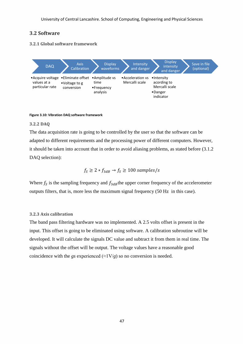
University of Central Lancashire. School of Computing, Engineering and Physical Sciences
47
3.2 Software
3.2.1 Global software framework
Figure 3.10: Vibration DAQ software framework
3.2.2 DAQ
The data acquisition rate is going to be controlled by the user so that the software can be
adapted to different requirements and the processing power of different computers. However,
it should be taken into account that in order to avoid aliasing problems, as stated before (3.1.2
DAQ selection):
2 ∗ 100 𝑚
Where is the sampling frequency and the upper corner frequency of the accelerometer
outputs filters, that is, more less the maximum signal frequency (50 Hz in this case).
3.2.3 Axis calibration
The band pass filtering hardware was no implemented. A 2.5 volts offset is present in the
input. This offset is going to be eliminated using software. A calibration subroutine will be
developed. It will calculate the signals DC value and subtract it from them in real time. The
signals without the offset will be output. The voltage values have a reasonable good
coincidence with the gs experienced (≈1V/g) so no conversion is needed.
DAQ
•Acquire voltage values at a particular rate
Axis Calibration
•Eliminate offset
•Voltage to g conversion
Display waveforms
•Amplitude vs time
•Frequency analysis
Intensity and danger
•Acceleration vs Mercalli scale
Display intensity
and danger
•Intensity acording to Mercalli scale
•Danger indicator
Save in file (optional)

University of Central Lancashire. School of Computing, Engineering and Physical Sciences
48
Figure 3.11: Calibration subroutine flowchart
3.2.4 Earthquake intensity and danger
Figure 3.12: Magnitude and danger calculator subroutine
Waveforms input
Calculate DC values
Subtract Dc values
Output signal w/o DC
BEGIN
END
BEGIN
X and Y axes ac. input
Select X and Y ac. range
XIntensity>Yintensity
Decode X and Y Mercalli scale
intensity
M.Intensity=X intensity M. Intensity=Yintensity
END
M.Intensity output

University of Central Lancashire. School of Computing, Engineering and Physical Sciences
49
The PGA and the intensity are related (PREPA.R.E, 2008). The detailed relation can be seen
in 2.1.5 Acceleration, intensity and damage. The subroutine should recognise the acceleration
range of each of the axes and identify the Mercalli intensity in real time. The axis with the
higher intensity determines the final result.
3.2.5 Display characteristics and saving options
The display should have a proper zooming or autoscalling options to study the input signals in
detail. Absolute time axis would be suitable. The danger indicator will indicate the Mercalli
intensity scale danger in real time. For each execution another indicator should display what
was the maximum intensity experienced during the current run. The user will select whether
and when to capture the waveform data that is being displayed by clicking a saving button.

University of Central Lancashire. School of Computing, Engineering and Physical Sciences
50
4. Seismological data analysis software design
4.1 Introduction and Specifications The objective of this part of the project is to develop software that performs the tasks below.
Figure 4.1 Seismic analysis software specifications
An important portion of this section consists of high-level flowcharts, as well as notes if
necessary. LabVIEW is a really high-level programming language as so they are the
flowcharts. There is no need to enter into low-level programming when the software has those
processes automatized. This section aim is to briefly describe and justify the design options
adopted.
4.2 Data format selection
When analysing the project requisites, the first problem that was encountered was what
seismic data format to use and whether it was freely distributed or needed to be requested to
the proper institutions. An important research work needed to be made in order to gather
information about seismic data and sources. A good amount of this information is available in
the seismic background section.
Although the SEED and miniSEED data formats are probably the most popular types, the
SEED format is an exchange format, what is to say, it stores absolutely all the data of the
event (Havskov & Ottemöller, 2010). According to the purposes and scope of the project, a
waveform (or processing) data type is more than enough; it was not recommendable to add
complications until the basic requirements were completed. In any case, although miniSEED
Specifications Decode seismic data from a standard format
Display waveform
Calculate relevant parameters: S-P arrival time, magnitude, epicentral distance, coda length.
Signal to noise ratio analysis(STA/LTA)
Manual and automatic phase picking
Optional filtering
Display frequency response
Interactive menu

University of Central Lancashire. School of Computing, Engineering and Physical Sciences
51
is part of that group, National Instruments does not provide a plug-in in their support website.
National instruments do provide numerous strong motion data plug-ins, including another
standard for a processing format; the SAC data format (National Instruments, 2011). Hence,
SAC format was used to process the data in this project as it is possible to obtain this type
directly and very easily from the biggest database found, IRIS. Not only that, the British
Geological Survey offers its earthquake data in this format too. This is particularly useful
because it allows the retrieval of local data. (British Geological Survey, 2012)
4.3 Global software framework
Figure 4.2: Global computation framework (Attri R. K., 2005)
The figure above represents the software structure. The process is controlled by the user,
deciding in which step should be picked up. Some phases need data from previous processes
so the user should be careful and know what it is being done. In any case, indications will be
included to help users not familiarized with seismic analysis. As we are using recorded digital
data, obviously a triggering process is not necessary.
4.4 Reading SAC files
Read data
•Retrieve properties
•Recover waveform
Optional frequency analysis
Optional band pass
filtering
Time parameters
•S arrival time
•P arrival time
•Coda length
•S-P time interval
Location parameters
•Distance to the epicenter in degees
•Distance to the epicenter in km
Magnitude aproximation
•Coda Magnitude(Mc)
•Surface Magnitude(MS)
Beginning
Retrieve
waveform
Decode
data
Retrieve
properties
End
Figure 4.3: Read data flowchart

University of Central Lancashire. School of Computing, Engineering and Physical Sciences
52
The plug-in has to carry out the decoding. The SAC files, as explained in the background,
include a waveform and headers with properties as the event date or the name of the seismic
station. Those also need to be retrieved to be displayed.
4.5 Frequency analysis and optional filtering
Sometimes it may be necessary to filter the seismograms, for example for a better phase
arrival timing (Havskov & Ottemöller, 2010).The software should include an option to filter
the waveform. Havskov et al (2010) recommends 4 order Butterworth filters. In order to
properly select the cut-off frequencies a tool to display the spectra would be really useful. The
seismic events have a typical low frequency so in this case a logarithm frequency scale is not
necessary.
4.6 Arrival times
4.6.1 Introduction
A system to automatically detect the wave arrivals is going to be developed due to the
importance of these parameters – described in seismic background (2.3.6.1 P and S arrival
times). One of the algorithms available to perform this task need to be applied but also a
manual picking tool is necessary.
4.6.2 Automatic picking
4.6.2.1 Algorithm selection
Among the available algorithms, the time domain energy based algorithms appeared to
simplify the tasks, featuring an acceptable accuracy. The STA/ LTA ratio method was
selected because of its simplicity and popularity (Han, 2010). Refer to STA/LTA ratio
description in the seismic background to see the algorithm detailed description.
=∑
Short-term average
=∑
Long term average
STA LTA ratio =STA/LTA
Equation 4.1: STA/LTA ratio equations

University of Central Lancashire. School of Computing, Engineering and Physical Sciences
53
As it is explained in the background there are different expressions for this method. The
expressions above present these advantages:
1) They can be calculated using data from one station only. Recall that a SAC data
file only incudes one waveform.
2) The expressions do not include square-roots as other do. The calculations have to
be performed, sometimes, in thousands of points. Eliminating one of the
operations can results in a significant improvement on performance.
In contrast, it does not have the precision of other algorithms (Han, 2010). Nevertheless,
considering the scope of the project it is far enough.
4.5.2.2 Flowcharts
If there is a proper preprogramed VI in among the available in LabVIEW to perform the
calculation it will be used, in any case the following diagram represents the programming
structure designed for its later LabVIEW implementation.
Figure 4.4: Automatic Arrival time picking global flowchart
Beginning
Initialisation:
-Retrieve user defined
parameters
-Retrieve signal data
STA /LTA ratio Pick arrival times
Display & Save data
End

University of Central Lancashire. School of Computing, Engineering and Physical Sciences
54
Figure 4.5: STA/LTA ratio implementation subroutine flowchart
Beginning
Initialisation:
-Retrieve user defined
parameters
-Retrieve signal data
-Retrieve sample number
Cut out windows values for the
indicated sample number
Calculate STA/LTA for window values specified
Save data
End
Beginning
Initialisation:
-Retrieve user defined parameters
-Retrieve signal data
STA/LTA one sample
calculator
Build & save waveform
Display point
No more
samples
End
YES
NO

University of Central Lancashire. School of Computing, Engineering and Physical Sciences
55
4.6.3 Manual picking
It was stated in the STA/LTA ratio description that the automatic picking has a great
dependence on the station and type of event sensed. If there is not data available or there is
not enough time to proceed with that calibration, the automatic picking is useless. Sometimes,
the seismograms available contain too much noise in the same bandwidth than the signal,
making difficult the correct functionality of modest automatic picking software like in this
case. These problems are common even in advanced professional software and sometimes are
compensated averaging the timing information of several channels available in the same
station (Munro K. A., 2005). However, in this project only one waveform is available. The
distance and magnitude calculations depend on the timing parameters so an alternative
method is required so that the analysis does not reach a dead-end. The software should allow
easy manual pickings using a cursor or similar techniques.
4.7 Coda length This parameter has significance enough to develop a subroutine that performs the task. The
method followed to design that subroutine is showed in the next page.
Beginning
Initialisation: -Retrieve user defined parameters -Retrieve signal data
Detect points over threshold
P time=first point S time=second point
S-P
Save & display data
End
Figure 4.7: Pick arrival times subroutine
Figure 4.6: STA/LTA one sample subroutine flowchart

University of Central Lancashire. School of Computing, Engineering and Physical Sciences
56
The P arrival time indicates the earthquake start. The software has to determine when the
event is finished, when the earth has calmed down (Attri R. K., 2005). It is known that LTA
values characterise a measurement of the noise level (Munro K. A., 2005). Therefore, it can
be used to determine an event conclusion. This happens when the current LTA levels are
compared with an average value before an event was triggered. If current LTA ≤ LTA
(averaged before P), the noise level is back to what it was before there was an earthquake.
The duration or coda length can be calculated with a simple subtraction.
𝑡 = 𝑖 𝑡𝑖𝑚 − 𝑡 𝑖 𝑡𝑖𝑚
Equation 4.2:Coda length
4.8 Distance to the epicentre
The habitual computational location methods used in professional stations around the world -
iterative approaches - are far over the scope of this project, not only because of the difficulty
of the implementation but because data from more than one station is required. Recall that
this project aim is to retrieve information from one seismogram at a time only. Moreover, the
task is to calculate the distance from the epicentre not locate the exact coordinates in 3D as
the mentioned approaches are able to do. (Havskov & Ottemöller, 2010).
Beginning
Initialisation:
-Retrieve P arrival time
-Retrieve LTA data
Pre-event LTA waveform average=threshold
Cut out LTA waveform
from P arrival time
Save Coda and final time
End
First value below time=final time
P arrival time-Final time=Coda length
Gather values below threshold
Figure 4.8: Coda lengthy subroutine flowchart

University of Central Lancashire. School of Computing, Engineering and Physical Sciences
57
In order to calculate this distance with a single seismogram there are two options. Using
lookup tables or approximation algorithms. (Attri R. K., 2005)A priori the incorporation of
these tables in the software looks like the most precise way to realise the software. However,
the integration of these tables in the software could represent an important amount of time
and even more if depth wants to be taken into account in order to make the most of this
procedure. Prior the programing of these tables the approximation equations have been tested
manually resulting in an error range of less than 1 ˚ in most of the cases up to a distance of
100 ˚. For events in a 2000 km range the inaccuracy was often around 0.1˚.The precision has
been considered acceptable for the objectives of the project. This approach saves lots of hours
of programing and table lookups in the internet.
Recall that the equations implemented, depending on the distance, are
1) From 0 to 250 km 𝛥 𝑘𝑚 = 𝑡𝑝𝑎 − 𝑡𝑠
𝑎 𝑣𝑝∗𝑣𝑠
𝑣𝑝−𝑣𝑠
𝑠 = 𝑝
√
= 𝑘𝑚
=
𝑘𝑚
𝑚 𝑡
2) From 250 km to 2222 km (20˚) 𝛥 𝑘𝑚 = 𝑡𝑝𝑎 − 𝑡𝑠
𝑎 ∗ 10
3) From 20˚ 𝛥 ˚ = [ 𝑡𝑝𝑎 − 𝑡𝑠
𝑎 𝑚𝑖 − 2] ∗ 10 [t] = minutes
Where 𝑡𝑝𝑎 and 𝑡 𝑠
𝑎 are P and S first arrivals respectively and Δ is the distance to the
epicentre.
Notice that from 9˚ to 20˚ and over 100˚ theoretically the algorithm is not valid. In the
evaluation section the magnitude of the probable inaccuracies will be tested. (Havskov &
Ottemöller, 2010)
The software will be based on the following structure:

University of Central Lancashire. School of Computing, Engineering and Physical Sciences
58
4.9 Magnitude
Among the several magnitude scales it was decided to use Mc and MS. Mc is an
approximation of ML (known as Richter scale) but the application is much simpler. Both Mc
and ML are local Magnitude scales so the programing of another magnitude that extends the
application range it is appropriate. Although, only for swallow events, Ms expands this range
up to 160 ˚ for magnitudes from 2 to 9 (Havskov & Ottemöller, 2010). Its application in
LabVIEW looks a priori simple because it only requires a filter and a peak detector, it has one
of the highest application ranges among the scales available and, moreover, it is
recommended by the BGS (British Geological Survey, 2011). For detailed Magnitude scale
range limitations see background.
Beginning
Initialisation: -Retrieve S-P time interval
Equation 1
NO
End
Equation 2
Equation 3
YES
YES
NO
Save distance (degrees and km)
Δ≥250 km OR Δ≥20 ˚
Δ≤20 ˚
Figure 4.9: Epicentre distance subroutine flowchart

University of Central Lancashire. School of Computing, Engineering and Physical Sciences
59
Figure 4.10: Magnitude calculations flowchart
Beginning
Initialisation: -Retrieve seismogram -Retrieve coda length
-Retrieve location
parameters
Mc calculation
Seismogram filtering (T= 2s-60 s )
End
Calculate MS(nm/s)
Detect maximum amplitude
Calculate MS(µm/s)
Save MS and Mc)
User defined Parameters:
-Mc local parameters -Seismogram Units
[nm/s] or
[µm/s]

University of Central Lancashire. School of Computing, Engineering and Physical Sciences
60
5. Analogue output design
Figure 5.1: Analogue output specifications
Figure 5.2: Analogue output flowchart
A subroutine to read the data will be developed; the one created for the seismic analysis may
be reusable. A user controlled linear scaling is going to be included. The fact that is
controlled by the user implies that the operator should be aware of the output voltage
limitations but, on the other hand, the real amplitude is always known, something that doesn’t
happen if the system automatically scales to eh maximum values. This program is meant to
display both acceleration and velocity waveforms so the operator should indicate what unit is
using. The output should be able to be paused and restarted at any time. Output pre-sets
subroutine has to retrieve critical parameters for the signal output as the output rate, buffer or
maximum and minimum voltage values.
Analogue output
Read and decode real seismic data
Analogue output of the data
BEGIN
Read file
Display data
Waveform output
END
Output pre-sets
Linear scaling

University of Central Lancashire. School of Computing, Engineering and Physical Sciences
61
6. Vibration monitoring system construction and implementation
6.1 Hardware Preliminary tests have been performed using the ADXL203 evaluation board and
oscilloscopes. Once the PCB was manufactured, the different connectors, a header and a
switch have been manually soldered. When the tracks connections were tested the
accelerometer was included
.
Figure 6.1 Vibration sensor device without the lid and header on which the evaluation board is mounted
The header inclusion possibilities the accelerometer substitution in case of failure. The header
connections were confirmed to be loose, slightly moving when the device is shacked, this
involves performance problems because the system is meant to be a high sensitive vibration
system. Hence, the accelerometer was placed and attached on the 4mm banana sockets using
easily removable adhesive in order to provide stability.
The PCB is fastened to the enclosure with instant adhesive to guarantee a satisfactory
vibration wave transmission. Holes have been cut out from the enclosure so that the supply
and input signal jacks can be connected. The already mentioned double-sided tape has been
applied.
Figure 6.2: Complete vibration sensor module.

University of Central Lancashire. School of Computing, Engineering and Physical Sciences
62
6.2 Software The user should select the data acquisition sample rate and buffer size, the data acquisition is
made by the DAQ assistant in order to save time as long as its limitations doesn’t bound the
design requisites. Acquire and pause buttons control the running. Big differences between the
sample rate and buffer size may cause issues so the operator should be careful. Too big
buffers can provoke excessive memory usage and crash. Do not exceed DAQ card sample
rate capabilities. The axes calibration VI filters the axes offset values, it requires separate
axes input so the DAQ dynamic data should be previously unbundled.
Figure 6.3 code section comprising DAQ assistant and calibration VI
Figure 6.4: Vibration DAQ front panel

University of Central Lancashire. School of Computing, Engineering and Physical Sciences
63
Spectra and acceleration time response are displayed in real-time for each of the axes. A chart
instead of a graph was believed to be more suitable for the time response. The VI displays the
instant and maximum Modified Mercalli intensity scale. The maximum intensity is saved
during execution but it initialises to 4 in each run. When considered appropriate, the operator
can decide whether to save the axes acceleration vs. time. The data format will be LVM and
the file is overwritten if there is previous data. LabVIEW graphs allow taking function
snapshots when running.
The Intensity and danger Display VI uses the axes absolute acceleration values and
determines to what intensity range the acceleration corresponds. The axis with the maximum
intensity determines the earthquake intensity final value.
Figure 6.5: "Intensity and danger Display" VI in the vibration DAQ main code
For more information, the complete code can be found in Appendix B.

University of Central Lancashire. School of Computing, Engineering and Physical Sciences
64
7. Seismological data analysis software implementation
In this section general comments about the main LabVIEW structures used are going to be
made. The Appendix A contains the whole code with more detailed explanations.
Figure 7.1Seismic analysis VI front panel
In order to read and decode the data files, a subVI called ReadSAC has been developed. It
retrieves the SAC file waveform and properties. The Open Data Storage express VI allows
opening external types of files when the data plug-in is available, once it is installed, it can be
selected in its dialog box. After the decoding, the file can be read with Read Data in channel
mode returning the seismogram waveform as dynamic data. To obtain the properties was
more problematic and it required the creation of another SubVI called RetrieveProperties. It
is based on the Get properties VI example available in the Labview 2010 data base (National
Instruments, 2010) and it uses For loops and the Get Properties VI to obtain metadata from
the file, channel groups and groups. Waveform and data are displayed in the seismic analysis
front panel. Notice that most of the data obtained does not inform in the properties about the
amplitude units so it is impossible to programmatically display them. The unit information
depends on the source and, therefore, a selector has been built-in so that the operator selects
the units of the waveform that has read .It is usually nm/s or µm/s (IRIS, 2011) (British
Geological Survey, 2012). With respect to the calculations this selections only affects to MS.

University of Central Lancashire. School of Computing, Engineering and Physical Sciences
65
Figure 7.2Code sections where the mentioned SubVIs are used
A subVI was created to calculate and show the seismogram vs. spectra. A dialog box opens
showing both graphs in a window separated from the seismic main controls and indicators.
Spectra magnitude is linear so that it can be compared in a better way with the seismogram,
the usually low bandwidth of typical earthquakes advices a linear frequency axis scale.
Figure 7.3 Seismogram and its spectra
The operator can define the low and upper cut-off frequencies of a band-pass filter. The
resulting filtered waveform is saved in a shift register so all the analysis operations can be
performed to the filtered signal. The LabVIEW filter VI can be set to use a 4 order

University of Central Lancashire. School of Computing, Engineering and Physical Sciences
66
Butterworth as recommended by Havskov et al. (Havskov & Ottemöller, 2010). Notice that if
the cut-ff frequencies do not fulfil the Nyquist criterion the software will return an error.
Figure 7.4 Filtering options in the seismic analysis front panel
In order to calculate the STA/LTA ratio, a proper pre-programmed VI was searched among
the VI’s available in LabVIEW. However, it was not possible to implement it in a satisfactory
way. It was considered that the development of an own subVI could save time and effort.
The subVI STA LTA wave (SNR) provides the STA/LTA ratio using window lengths selected
by the operator while Pick arrival times VI uses this ratio along with a user defined threshold
to automatically pick the P and S arrival timing.
Figure 7.5 : STA LTA ratio and Pick arrival times VIs in the main seismic code
The STA/LTA wave SubVI is set up in dialog mode so that a new window with its front panel
pops up when the automatic picking control is pressed. The use of different windows was
considered an appropriate way to expand the information showed in screen and to show the
user the state of the SNR calculations, as it take some seconds until it is completed.

University of Central Lancashire. School of Computing, Engineering and Physical Sciences
67
Figure 7.6 STA/LTA ratio VI front panel. The figure shows an earthquake seismogram, the STA/LTA ratio and the STA and LTA waves for specific L1 and L2 window lengths
The SNR calculations are performed sample by sample by a VI called STA LTA one sample.
Basically, the STA LTA ratio VI function is to control the running of that other subVI,
window lengths and to put together the waveform. The Pick arrival times VI takes advantage
of the fact that the first two values that surpass the threshold value are, respectively, the P and
S arrival times. Arrival time values are actualised when STA LTA ratio dialog box is closed.
Detailed comments are written in Appendix A.
The manual picking has been carried out using three vertical cursors which display the time
axis values. To use this tool the user should manually identify and introduce the correct P and
S arrival time values as well as the end of the event time in the proper controls before
proceeding with further automatic calculations. The subtractions required to determine S-P
time and coda length are automatically performed.

University of Central Lancashire. School of Computing, Engineering and Physical Sciences
68
Figure 7.7 Cursors and controls for manual picking in the seismic analysis VI front panel(left) and the loop that actualises coda length and S-P when the use modifies arrival times.
A coda length meter VI was developed in order to retrieve this magnitude. It performs the
actions described in the design section. It uses the LTA waveform and the P wave arrival time
to obtain the coda length and the event end time. In this case only the event end time is
retrieved as the final subtraction to calculate the coda ( P arrival time – event end time) is
performed in the main seismic analysis VI in order to allow the user to manually change the
event end time at any time (manual picking). The automatic coda results are actualised at the
same time that the arrival times. A subVI called Gathering Signal Values below a Threshold
value is used. This design is a modification of Gathering Signal Values passed Threshold
value VI developed by one of the NI Instructors in the NI developer zone. It is available to
public (NI Instructors, 2011). Detailed description in appendix A.
Figure 7.8 "Coda length" VI in the main seismic code
The Distance to the epicentre VI uses the P and S arrival times – previously calculated or
manually typed - and the already known P and S wave speed - in a normal crust – to
determine the station distance to the epicentre in km and degrees. Empirical formulas are used.
Notice that the algorithm should change depending on the event distance; this is achieved
with a case structure. Values are returned and displayed in the main seismic menu; no dialog
box is opened when running.

University of Central Lancashire. School of Computing, Engineering and Physical Sciences
69
Figure 7.9: Distance to the epicentre subVI placed in the seismic analysis code.
When Calculate magnitude button is pressed in the front panel, the system processes the
seismogram, coda length and distance to the epicentre parameters – that should be previously
settled – to calculate the MS and Mc magnitude. To calculate Mc , a, b and c parameters
should be input by the user and a coda length value has to be available. MS requires previous
bandpass filtering (2 to 60s) as indicated in the background. The maximum value of the
filtered signal, as well as the epicentral distance in deg, is used to compute this magnitude
scale. The user can select the signal units so that the formula rearranges for correct calculation.
The block diagram can be seen in the Appendix A.
Figure 7.10: Magnitude controls and indicators in the front panel
8. Analogue output software implementation
An analogue output VI has been developed. The software is able to read LVM files,
containing acceleration time response, and SAC files, it auto detects the input format. There is
a user controlled linear scaling. The output start and pause is user managed. When scaling,
the output must be within the configured max and min voltage. In this case +-10 V. As
different type of data may be read, the user should manually indicate the amplitude units. The
DAQmx auto start function should be on to avoid overwriting errors (-200279) when starting
the output after stopped (National Instruments, 2012).Output presets VI defines the output
task characteristics, in this case, outputs the signal at 50 kHz using a 10 samples buffer. High
buffers may cause errors.

University of Central Lancashire. School of Computing, Engineering and Physical Sciences
70
Figure 8.1: Analogue output VI front panel
9. Dataflow and Interface The interface and data flow has been managed using mainly the event structure. The events
are usually buttons pressed. When that happens the program jumps to different running
points. Shift registers save event common data while the VIs is running, like the seismogram
or errors. Although they are a resource many times avoided, local variable have been required
so that controls can be changed both automatically and manually by the user, for example, the
P arrival time control can be set by the user but when it is calculated automatically the new
value actualises the control through a local variable. SubVIs have been created to perform
tasks in a more organized way. Generally, SubVIs were created after processes that were
considered important and independent enough to be called subroutines in the design chapter.

University of Central Lancashire. School of Computing, Engineering and Physical Sciences
71
Figure 9.1: Example of the event structure continuously used in the software. The External loop keeps it running. The shift registers and local variables can be seen.
Figure 9.2: Main menu interface
All the front panels used as interface front panels are included in the Appendixes along with
the VIs block diagrams. The Appendix D comprises some usage instructions.

University of Central Lancashire. School of Computing, Engineering and Physical Sciences
72
10. System evaluation and results
10.1 Vibration DAQ evaluation The figure below shows the hardware configuration in the tests performed. Note the BNC
input connected to the vibration module and the analogue output connected to the
oscilloscope trough a BNC coaxial wire.
Figure 10.1: Hardware system distribution for vibration DAQ and output testing
Prior to the insertion of the accelerometer analogue outputs into the NI2120 they were tested
in an oscilloscope to ensure that de device is not defective.
Figure 10.2: Accelerometer voltage outputs when tilted so that the two axes support different accelerations
The vibration DAQ has been tried for different vibration conditions using a 12 kS/s sample
rate and a 1000 samples buffer size. Previously, the intensity indicator was tried out with
simulated signals to assure that it indicates the correct level. The tests were carried out

University of Central Lancashire. School of Computing, Engineering and Physical Sciences
73
attaching the vibration module to a table and applying different magnitude vibrations, hits,
and shakings.
Figure 10.3: DAQ front panel when running
Figure 10.4: Light table hitting (Y axis) time and frequency responses

University of Central Lancashire. School of Computing, Engineering and Physical Sciences
74
Figure 10.5: Strong enclosure hitting (X axis) time responses
Figure 10.6: Strong shaking time and frequency responses

University of Central Lancashire. School of Computing, Engineering and Physical Sciences
75
Figure 10.7: Heavy shaking time and frequency responses
The saved files were successfully opened using the analogue output VI that is going to be
later analysed.
It appears that the system is working well showing coherent responses to the different
excitations. It proved to be really sensitive, responding to really light finger tapings. More
exhaustive analysis may be needed in the future.
10.2 Seismic analysis evaluation
The software successfully decodes and reads SAC data. The seismogram waveform was
displayed successfully in a 100% of the tried data. The property reading varies depending of
the data source; some sources provide parameters that other don’t. A failure in National
Instrument’s plug-in has been detected as some of the dates are not displayed correctly. The
software successfully reads the metadata that has been considered appropriate and that is
commonly present in main providers’ files (see Seismic analysis implementation). Critical

University of Central Lancashire. School of Computing, Engineering and Physical Sciences
76
parameters for the software development like the time delta or total samples are not always
included in the metadata, therefore, the program obtains them analysing the characteristics of
the incoming data. The station coordinates are either not included or the plug-in is unable to
acquire them, this represent a major inconvenience because it limits the possibility of
calculating and plotting the earthquake epicentre coordinates if seismograms from 3 different
stations were available (Attri R. K., 2005).
As it can be appreciated, the data properties displayed in my software match the ones in the
data file viewer VI provided by LabVIEW.
Figure 10.8: Properties in Data file viewer
The epicentre distance algorithm has been tested using the travel time tables provided by the
US geological survey. These tables, often presented as graphs, relate the S-P time interval to
the distance of the event in degrees or km. The figure below compares the distance calculated
for an established S-P time interval with the distance in the chart for the same time interval.
Recall that the relation between S-P time and distance depends on the depth. The table study
33 km depth events and, although the software implemented is a good approximation,
supposes surface events, consequently, the shallower the earthquake the more precision it
provides.
Figure 10.9: Data properties in seismic software

University of Central Lancashire. School of Computing, Engineering and Physical Sciences
77
Figure 10.8 Software distance calculations compared to USGS Distance vs S-P time table
The results surpass the theoretical strength of the algorithm used. Notice that, between 1000
km (9˚) and 20˚, there was a gap where there was not a proper algorithm available. In view of
the situation, the equation used from 250 km to 1000 km was extended to that breach with
satisfactory results. As expected, over 100 ˚ there is a worse performance. However; in most
of the cases below that distance the divergence rarely exceeds 3˚.
To test the software magnitude calculations, the results have been compared with the ones
provided by IRIS (IRIS, 2011). They are represented in the figure below along with some
other values related to the software limitations. There was a preference for local data,
however, most of the data from the British Geological Survey page comes from non-
professional networks and it was difficult to find clean seismograms with an acceptable SNR
in the professional networks available (British Geological Survey, 2012). Therefore, the
alternative chosen has been the Japan Meteorological Agency Seismic Network because it
provides extensive and varied earthquake data due to the region activity. Besides, the signal’s
SNR is usually high allowing an ideal study of the signals. Its data is available from IRIS
using the WILBER II tool for seismic data downloading.
0
20
40
60
80
100
120
0 200 400 600 800
Dis
tan
ce(d
eg)
S-P time(s)
Distance(USGS)
Distance(software)

University of Central Lancashire. School of Computing, Engineering and Physical Sciences
78
Event Depth(km) Distance(˚) Magnitude(IRIS) Mc MS
2011/09/15 08:00:07.1
NEAR EAST COAST OF
HONSHU, JAPAN(JHJ2)
10 3.4 6.3 5.65 5.63
2012/03/14 09:08:37.5 OFF
EAST COAST OF HONSHU,
JAPAN(JHJ2)
26.60 8.56 6.8 8.4 6.9
2011/10/21
08:02:38.1 HOKKAIDO,
JAPAN REGION(JHJ2)
188.20 10.35 5.8 7.7 5.7
2011/06/26
09:19:48.2 MARIANA
ISLANDS (CBIJ)
99.90 8.38 5.7 7.07 5.07
2011/08/20
18:19:21.0 VANUATU
ISLANDS(YOJ)
2 65.5 7 30.59 7.06
2012/01/10 18:37:01.2 OFF
W COAST OF NORTHERN
SUMATERA
29.10 38 7.3 20.4 6.96
2011/09/18
12:40:48.1 SIKKIM, INDIA
20.7 46.09 6.8 23.59 6.86
2007/08/15 23:40:56.8 NEAR
COAST OF PERU
30.20 207.32 8 86.28
8.22
Table 10.1 Software magnitude calculations evaluation. Comparison with magnitude of different data retrieved from ISIS.
The manual picking function has been used to determine the arrivals. The equation
parameters selected for the Coda Magnitude determination are the ones determined by the US
Geological Survey in 1972 (W.H.K Lee et al, 1972). It was not possible to find these

University of Central Lancashire. School of Computing, Engineering and Physical Sciences
79
particular parameters for the Japan region. Nevertheless, some references indicated that the
parameters are still used nowadays for the detection of earthquakes in places where there are
not coda magnitude studies or they cannot be found (Havskov & Ottemöller, 2010) (Kayal,
2008).
From these results it can be stated that:
MS is a good approximation for relatively shallow earthquakes
In really short and long distance events generally MS lacks accuracy
Really deep events also reduce MS accuracy.
It shows why the coda magnitude is discredited (Havskov & Ottemöller, 2010), it is an
approximation to Richter magnitude in local events but as it can be seen, it is not
working properly. For long distance earthquakes it is not even close.
The results match with the theoretical specification that was known when implemented. MS
works well with events in a distance range from 2˚ to 160˚ and less than 60 km depth. Mc is
an approximation for local events but it didn’t work well in this case. It is not a good method
when using manual picking because of its critical dependence on coda length. Also, the
generic expression by Lee et al has been used because a particularization for the expression
has not been found for Japan, probably that contributed to its bad performance in the studied
cases.
In order to confirm this aspect a test has been performed using data from the Oregon
University Network and Coda Magnitude parameters for the adjacent California.
Event Depth(km) Distance(˚) Magnitude(IRIS) Mc
2011/09/09 19:41:35.0
VANCOUVER ISLAND
REGION
25.90 5.8 6.7 6.9
Table 10.2 Coda magnitude characteristics verification
The result corroborates a great improvement compared to the previous coda Magnitude
values.
The system successfully displays the LTA, STA and its ratio, therefore, a SNR measurement
is available for its study. The graphs built show a ratio growth when there is an incoming
signal - P and S wave respectively. Occasionally there may be other peaks due to the

University of Central Lancashire. School of Computing, Engineering and Physical Sciences
80
incoming surface waves or particularly intense noise. Notice that this happens often in far
events due to the wave speed difference which tend to separate surface waves from S signals.
The software was intended to use this information to automatically calculate the P and S
waves arrival times – in this text sometimes denoted as automatic phase picking. Before the
performance of this part can be evaluated, a process of calibration must be performed. The
threshold that determines the wave arrival has to be defined depending on the station that
makes the measurements. These calibration processes are made taking into account the station
history (Attri R. K., 2005), however, for obvious reasons the one that is included in this report
doesn’t cover that extension. The threshold values have been calculated averaging 16 different
thresholds from 8 different events.
Figure 10.9: STA/LTA ratio VI front panel

University of Central Lancashire. School of Computing, Engineering and Physical Sciences
81
The process followed comprised these steps for each of the events:
1) Manual picking
2) Selecting L1 an L2 windows depending on the signal frequency response.
L1 = 3*expected signal period; L2=10*L1.Frequency analysis performed with the
previously developed software function.
3) SNR study, pick the threshold value that provides an arrival time that matches with the
manual picking. For both P and S waves.
A history chart was made and averaged to obtain a proper threshold value.
Probably, trimming could be performed by statistically adjusting L1 and L2 for each event
based on the manual pickings (Munro K. , 2004) but is out of reach with the available time.
The calibration has been made for the station JHJ2 based in Hachijojima Island belonging to
the Japan Meteorological Agency Seismic Network. Again, the reason is the amount of events
to choose from after the March 11 earthquake and the clarity of the seismograms available.
EVENT MAN(P)[s] MAN(S)[s] L1 L2 Tp Ts
1) 2012 02 14 NEAR EAST COAST
OF HONSHU JAPAN 84.54 123.98 3 30 3.1 3.1
2) 2011 10 21 HOKKAIDO, JAPAN
REGION 96 209.35 3.75 37.5 2.6 2.4
3) 2011 12 09 SEA OF OKHOTSK 89.12 245.58 3 30 2.9 3.7
4) 2011 08 01 NEAR S. COAST OF
HONSHU, JAPAN 84.54 109.59 6 60 2.9 5.5
5) 2011 07 23 NEAR EAST COAST
OF HONSHU, JAPAN 84.55 143.8 7 70 2.7 2.1
6) 2011 04 01 EASTERN
HONSHU, JAPAN 86.46 151 6 60 3.2 2.2
7) 2011 04 07 NEAR EAST COAST
OF HONSHU, JAPAN 90.56 149.56 7.5 75 3.2 1.8
8) 2011 04 28 NEAR EAST COAST
OF HONSHU, JAPAN 85.73 134.33 7.5 75 1 1.7
Table 10.3Threshold determination for different earthquakes

University of Central Lancashire. School of Computing, Engineering and Physical Sciences
82
The following chart displays different threshold values and averages them.
Figure 10.10: Averaged threshold
The average value T=2.775 was used to test the automatic phase picking software. The
automatic arrival values are compared with the manual picking ones. L1 and L2 are the same
indicated in the previous table.
EVENT MAN(P)[s] AUT(P)[s] MAN(S)[s] AUT(S)[s]
1) 2012 02 14 NEAR EAST COAST
OF HONSHU JAPAN 84.54 84.1 123.98 123.6
2) 2011 10 21 HOKKAIDO, JAPAN
REGION 96 96.05 209.35 209.65
3) 2011 12 09 SEA OF OKHOTSK 89.12 89 245.58 245.35
4) 2011 08 01 NEAR S. COAST OF
HONSHU, JAPAN 84.54 84.5 109.59 -
5) 2011 07 23 NEAR EAST COAST
OF HONSHU, JAPAN 84.55 84.65 143.8 144.55
6) 2011 04 01 EASTERN
HONSHU, JAPAN 86.46 85.6 151 151.7
7) 2011 04 07 NEAR EAST COAST
OF HONSHU, JAPAN 90.56 90.55 149.56 151.35
8) 2011 04 28 NEAR EAST COAST
OF HONSHU, JAPAN 85.73 7.5 134.33 136.5
Table 10.4: Automatic and manual picking comparrison
2.775
1
1.5
2
2.5
3
3.5
4
4.5
5
5.5
1 2 3 4 5 6 7 8 9 10 11 12 13 14 15 16
Títu
lo d
el e
je
Título del eje
Thresholds Average threshold

University of Central Lancashire. School of Computing, Engineering and Physical Sciences
83
The results are mostly satisfactory for the number of arrival threshold that have been
averaged, the error rarely exceed 0.5 seconds. Number 7 and 8 S wave arrival appears to be
problematic probably due to the number of averaged sampled. However, number 8 is a really
noisy seismogram, there is apparently a bad influence of background noise in picking that this
algorithm is not able to solve. The generalized threshold – for both P and S picking – appear
to have also a negative effect compared to other studies found (Munro K. , 2004) reducing the
precision that could have been reached if using different values. In events with P and S waves
arrivals really close in time doesn’t work properly – earthquake 4.
This algorithm seem to be a good qualitative method to calculate approximated arrival times
with a precision of around 0.5 seconds –probably much less with the appropriate history
study. Nevertheless, fails to be the ultimate method to provide timings precisely with real
data. Kim Munro concludes the same in her study Automatic event detection and picking of
P-wave arrivals (Munro K. , 2004). An algorithm modification for improvement was
presented in her later Thesis Analysis of microseismic event picking with applications to
landslide and oil-field monitoring settings (Munro K. A., 2005).
The first STA/LTA software programmed had serious performance problems as the
processing of data comprising around 15’000 samples took between 40 and 50 seconds (Intel
Core i5 processor 2.3 GHz). By substituting express VIs and modifying the algorithm, that
time has been reduced to half. It is not a brilliant performance though. Performing the
window calculations point by point to such amount of data requires processing power.
However, it is considered that in the future a reduction in processing time is still possible with
the current implementation, especially regarding the resetting. In the current state it is not
recommendable to use the automatic picking with data over the samples indicated above. The
SNR ratio front panel pops up when using the automatic picking allowing the user to see the
calculation progress.
The coda length calculator present problems related to the algorithm, from the several test
performed only few gave satisfactory results. It is important to notice that the evaluation of
this piece of software was extremely difficult due to the subjectivity of the magnitude to
measure (Havskov & Ottemöller, 2010). The automatic detector is far more sensible than the
manual picking so it is was sometimes difficult to say if the problem was the user ability to
choose a proper coda or the software performance. However, the poor execution was evident

University of Central Lancashire. School of Computing, Engineering and Physical Sciences
84
with a naked eye due to some impossible results. The problem was identified and described
below.
Figure 10.11: Coda length calculator problem
The detection extremely depends on the correct P wave time arrival detection. The figure
above represents the LTA wave, the background noise. If the P wave timing is slightly
imprecise the VI “cuts out” the waveform before it was supposed. The remaining waveforms
values are later compared with a typical noise value before the earthquake arrival, notice that
if the remaining values contain pre-event noise levels the event end time picked is going to be
incorrect, far before than when it was supposed. As explained above, it is impossible to assure
a perfect automatic P or S arrival picking with the available resources, and the precision
required for the algorithm above may be tens of milliseconds- few samples make the
difference. This issue improvement will be one of the future works suggested. It is also
important to highlight that the data analysed has to include the samples where the earth is
settled down. This is not trivial, good amount of data samples available in the internet do not
include this information, they are cut out before, the waveform never returns to the pre-event
levels and, hence, the analysis always returns wrong values.
Wrong P arrival time
The software “cuts-out” the waveform from
here to perform a comparing task with the
remaining values. If P timing is wrong, the
remaining waveform contains pre-event
noise levels.
Wrong end time

University of Central Lancashire. School of Computing, Engineering and Physical Sciences
85
Other additional functions as the frequency analysis or the band pass filtering are working
correctly. The following charts correspond to a 2012 event near the east coast of Honshu.
Figure 10.12: Non- filtered seismogram
Figure 10.13: Seismogram spectra
Figure 10.14: Filtered seismogram. Low cut-off = 0. 01 Hz. High cut-off =1 Hz
By the time this report is being typed, some user interface issues are not still polished
causing occasional crashes but allowing the evaluation of the different VI’s developed. It is
expected that this issues are solved before the demonstration.

University of Central Lancashire. School of Computing, Engineering and Physical Sciences
86
10.3 Analogue output evaluation
The analogue output software successfully reads and outputs LVM files containing X or Y
axes acceleration recorded with Vibration DAQ VI and the designed hardware module. It also
works well with the SAC files (velocity) downloaded from the IRIS database. The stop,
refresh and scaling options don’t show problems if the operator works within the restrictions
stated in the implementation section.
Figure 10.15: Analogue output front panel running and reading a SAC file.
Figure 10.16: LVM vibration file reading and analogue output

University of Central Lancashire. School of Computing, Engineering and Physical Sciences
87
Figure 10.17: SAC file reading and analogue output
11. Future work: Potential improvements and modifications The project accomplishes most of the objectives that were set. However, when designing and
implementing the work, alternative development procedures and improvement ideas came up.
Unfortunately, as always, time and resources were limited and they had to be abandoned or at
least postposed in order to deal with the main objectives. Some of them are going to be
proposed in this section:
In order to monitor ambient noise in some structures as bridges a µg resolution is
required (Wenzel & Pichler, 2005). The addition of a second accelerometer that
measures acceleration in another axis may be a useful approach to improve the
hardware module so that can be used for that purpose.
An aisled vibration DAQ module has been developed. In order to study the large
structures vibration behaviour a good amount of them, distributed in strategic
locations, are needed (Wenzel & Pichler, 2005). The development of a decentralised

University of Central Lancashire. School of Computing, Engineering and Physical Sciences
88
networking system that uses, for example, microcontrollers would be suitable to
perform this task.
The seismic analysis VI analyses one seismogram at a time and the location
parameter that returns is the distance to the epicentre. It is possible to plot the
location when the distance from at least three different seismic stations is known. A
logical work continuation is the development of software that processes that
distance values and uses a graphic interface to plot the location on a world map.
The use of tables instead of formulas to calculate the distance to the epicentre
would improve that parameter precision.
The calculation of the magnitude using more scales would save the user time as
there would be no need to use conversion graphs (Havskov & Ottemöller, 2010).
Better algorithms for arrival time detection using wavelet transform or frequency
analysis among others could be integrated in the software (Han, 2010).
Coda length algorithm improvement to avoid the errors detected in its evaluation
STA/LTA average performance optimization. Another approach for its development
or an improvement of the existing one (the collector VI appears to be the cause of a
lot of this issue) is required.
In order to gather samples to shape a waveform only the collector VI has found
among the LabVIEW library. That VI is not only slow but also has the collected
samples limited. The development of a fast sample collecting VI without pre-
established sample number limitation would boost the improvement of the
STA/LTA average calculation performance.
Because of the time limitations, the main menu (event structure) that should have
joint the access to the three main software functions (DAQ, seismic analysis and
output) in a common interface could not be completed. Also, some bugs in the
seismic interface as occasional crashes without apparent reason were noticed. It is
expected that this issues are solved by the time of the demonstration.

University of Central Lancashire. School of Computing, Engineering and Physical Sciences
89
12. Conclusion
Monitoring and analysis of seismic signals have become a fundamental discipline when
trying to minimize the human and economic loss that earthquakes cause every year. To deal
with this menace, geologist need to be supplied with analytical tools that help with the
arduous work of determining the seismic event characteristics in order to take preventing
actions, establish patterns or study the earth structure. Preventing work has to be made in
building structures as well, cheap maintenance and failure detecting systems are highly on
demand and it is there where MEMS accelerometers plays a fundamental role.
The seismic analysis software developed manages to successfully retrieve timing, location
and magnitude parameters with an acceptable precision according to the scope of the project.
The precision achieved is probably not suitable for the accurate calculations of professional
seismic stations. However, taking into account the resources and time available and that the
geo-instrumentation and LabVIEW knowledge was acquired as part of the project, it
represents a good approach and prototype from which build up a more complex software
using this popular graphic programming language. It is important to highlight that the
software has performance issues when computing SNR analysis and automatic timing
parameters detection and that improve this in the future is essential. The coda length software
needs also polishing or algorithm reconsideration to avoid some calculations errors. The event
date that can be retrieved from the SAC_SM plugging does not match with the source date
too often; this might point out a problem with either the plug-in or the seismic data source.
The vibration DAQ effectively performs acceleration versus time and spectra measuring and
monitoring. It manages to translate the incoming acceleration into earthquake intensity rank
in accordance with the Modified Mercalli scale. Saving and zooming options are properly
working and the enclosure and double sided tape using for attachment fits very well the
specifications marked at the beginning of the development. Nevertheless, the user should be
careful with the sample rate and buffer selection as a wrong selection may cause conflicts
with the hardware. The system is a good starting point to develop a networked system for
structural monitoring.
The software manages to output vibration and seismic signals based on real data without
problems. This analogue output may be used to be read in an oscilloscope or to excite a
shaking table in order to simulate history-based earthquakes.

University of Central Lancashire. School of Computing, Engineering and Physical Sciences
90
Although an initial objective, the usefulness and practical applications of an analogue input
that acquires the analogue output commented above has been questioned. Especially when
digital data can be easily found in the internet and vibrations were already acquired with the
vibration DAQ. It could be interesting to simulate the real acquisition process that occurs in
professional seismic stations but, taking into account that the project is already branched in
different areas and the lack of time available it was decided to focus in the ones that looked
more valuable.
As a whole, the project reasonably accomplishes the objectives initially set, but it is evident
that the fields studied have a lot of potential and room for improvement .Complex and
valuable applications can be developed taking this work as a starting point.

University of Central Lancashire. School of Computing, Engineering and Physical Sciences
91
Appendix A: Detailed Seismic analysis software
Figure A. 1: Seismic analysis VI front panel
Figure A. 2: Seismic analysis VI global structure. Timeout event.

University of Central Lancashire. School of Computing, Engineering and Physical Sciences
92
Figure A. 3: Seismic analysis VI. Read file event
Figure A.4 Seismic analysis VI. Automatic picking event

University of Central Lancashire. School of Computing, Engineering and Physical Sciences
93
Figure A. 5: Seismic analysis VI .Frequency analysis event
Figure A. 6:Seismic analysis VI.Filter event

University of Central Lancashire. School of Computing, Engineering and Physical Sciences
94
Figure A.7: Seismic analysis VI. Calculate distance event
Figure A.8: Seismic analysis VI. Calculate magnitude event

University of Central Lancashire. School of Computing, Engineering and Physical Sciences
95
Figure A..9: Seismic analysis VI. Stop event.

University of Central Lancashire. School of Computing, Engineering and Physical Sciences
96
Figure A.10: Read SAC VI icon
Figure A.11: ReadSAC VI block diagram

University of Central Lancashire. School of Computing, Engineering and Physical Sciences
97
Figure A.12: Retrieve properties Icon
FigureA.11: Retrieve properties VI block diagram

University of Central Lancashire. School of Computing, Engineering and Physical Sciences
98
Figure A.3: STA LTA ratio icon
Figure A.12: STA LTA ratio front panel

University of Central Lancashire. School of Computing, Engineering and Physical Sciences
99
Figure A..13: STA LTA ratio VI Start event and global VI structure
FigureA.14:STA LTA ratio VI BACK event

University of Central Lancashire. School of Computing, Engineering and Physical Sciences
100
FigureA.15: STA LTA one sample VI icon
Figure A.16:STA LTA one sample block diagram

University of Central Lancashire. School of Computing, Engineering and Physical Sciences
101
Figure A.17: Pick arrival times VI icon
Figure A.18: Pick arrival times VI block diagram

University of Central Lancashire. School of Computing, Engineering and Physical Sciences
102
FigureA.19: Frequency analysis VI icon
FigureA.20: Frequency analysis VI front panel

University of Central Lancashire. School of Computing, Engineering and Physical Sciences
103
FigureA.21: Frequency analysis VI block diagram
Figure A.22: Distance to the epicentre icon
Figure A.23: Distance to the epicentre block diagram
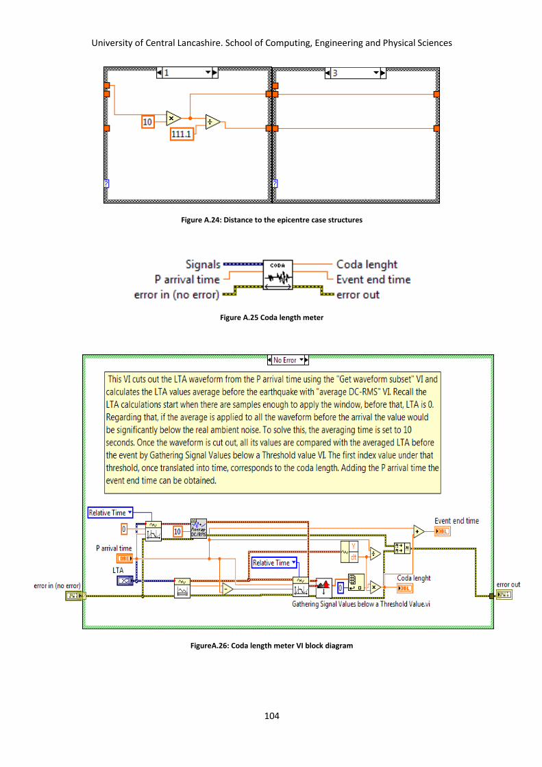
University of Central Lancashire. School of Computing, Engineering and Physical Sciences
104
Figure A.24: Distance to the epicentre case structures
Figure A.25 Coda length meter
FigureA.26: Coda length meter VI block diagram

University of Central Lancashire. School of Computing, Engineering and Physical Sciences
105
Figure A.27: Gather signals below a threshold VI icon
Figure A.28: Gather signals below a threshold block diagram (NI Instructors, 2011) .

University of Central Lancashire. School of Computing, Engineering and Physical Sciences
106
Appendix B: Detailed Vibration DAQ software
Figure B.1: Vibration DAQ VI front panel
Figure B.2: Vibration DAQ event structure. Timeout.

University of Central Lancashire. School of Computing, Engineering and Physical Sciences
107
Figure B.3: Vibration DAQ VI. Acquire event
FigureB.4: Vibration DAQ VI Main menu event

University of Central Lancashire. School of Computing, Engineering and Physical Sciences
108
FigureB.5: Vibration DAQ VI pause event
FigureB.6: Axes calibration VI icon
FigureB.7: Axes calibration VI block diagram

University of Central Lancashire. School of Computing, Engineering and Physical Sciences
109
FigureB.8: Intensity and danger display VI icon
Figure B0.9: Intensity and danger display VI front panel

University of Central Lancashire. School of Computing, Engineering and Physical Sciences
110
Appendix C: Detailed analogue output software
FigureC.1: Analogue output VI front panel
FigureC.2: Analogue output VI .Timeout event

University of Central Lancashire. School of Computing, Engineering and Physical Sciences
111
Figure C.3: Analogue output VI. Read file event.

University of Central Lancashire. School of Computing, Engineering and Physical Sciences
112
Figure C.4: Analogue output VI. Start output event.
Figure C. 5: Analogue output VI. Back event

University of Central Lancashire. School of Computing, Engineering and Physical Sciences
113
Appendix D: Brief Instructions for use
Figure D.1: Seismic analysis main window instructions
Reads or
actualises data Opens frequency
analysis window
Band pass filter. The
user should select the
cut –off frequencies Returns to
main menu
Selects file
to analyse
Cursors for
manual picking.
Use as a
reference to
identify arrival
and end times.
Automatically
calculates timing
parameters. L1,
L2 and threshold
required.
Prior to calculate the
distance, timing
parameters should
have been manually
or automatically
identified.
Coda magnitude
requires a, b and c
parameters. The
seismogram units
affect Ms calculations.
Previous distance data
required.
Graph
tools

University of Central Lancashire. School of Computing, Engineering and Physical Sciences
114
Figure D.2: STA LTA ratio VI front panel instructions
Press to start SNR
analysis. L1,L2 can be
redefined Return to menu Seismogram display
STA/LTA ratio waveform
display. Signal to noise
ratio
STA & LTA display.
Signal and noise
respectively

University of Central Lancashire. School of Computing, Engineering and Physical Sciences
115
Figure D.3: Vibration DAQ VI instructions
Start/continue
samples
acquisition
Pause
acquisition Return to main menu
Save time
response
Modify rate and
buffer
Intensity and danger
indicators. Instant danger
(left). Maximum danger
(right)

University of Central Lancashire. School of Computing, Engineering and Physical Sciences
116
Figure D.4: Analogue output VI instructions
Select file to
output. LVM
and SAC format
are admitted
Read or
refresh the
file
Start/continue
output
Pause/stop
output
Return to
Main menu
Select
amplitude
units
Linear scaling
factor
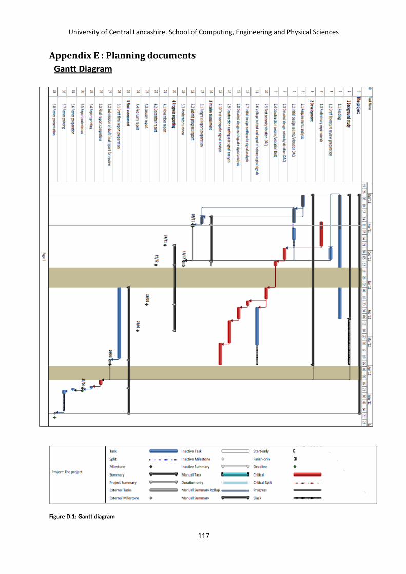
University of Central Lancashire. School of Computing, Engineering and Physical Sciences
117
Appendix E : Planning documents
Gantt Diagram
Figure D.1: Gantt diagram

University of Central Lancashire. School of Computing, Engineering and Physical Sciences
118
Risk register
Figure D.2: Risk register

University of Central Lancashire. School of Computing, Engineering and Physical Sciences
119
Appendix F: DAQ Circuit and PCB plans

University of Central Lancashire. School of Computing, Engineering and Physical Sciences
120

University of Central Lancashire. School of Computing, Engineering and Physical Sciences
121

University of Central Lancashire. School of Computing, Engineering and Physical Sciences
122

University of Central Lancashire. School of Computing, Engineering and Physical Sciences
123

University of Central Lancashire. School of Computing, Engineering and Physical Sciences
124

University of Central Lancashire. School of Computing, Engineering and Physical Sciences
125

University of Central Lancashire. School of Computing, Engineering and Physical Sciences
126
Appendix G: DAQ hardware components list
Description Manufacturer Package Quantity
Capacitor(100nF) Multicomp 0805 2
Capacitor (0.1µF) Multicomp 0805 1
ADXL203 MEMS
accelerometer
Analogue Devices 5mm x 5mm x
2mm LCC
1
ADXL203EB
Evaluation Board
Analogue Devices - 1
C1553ATNAE
Switch
Archoelectric
switches
- 1
2.1 DC Jack Dongguan
HaoyuElectronics
- 1
MP-205 2.1 DC plug
Multicomp - 1
4mm Banana jack Multicomp - 2
NI 6021DAQ card National Instruments - 1
BNC 2120
Connector socket
National Instruments - 1
PCB UCLAN - 1
1591XXMS General
purpose enclosure
Hammond
Manufacturing
1
BNC Lead(BNC
plug-4mm banana
plug)
- - 2
5 way 2.54 mm
header
- - 1
Double sided tape - - 1
Superglue - - 1
Table G.1 DAQ hardware component list

University of Central Lancashire. School of Computing, Engineering and Physical Sciences
127
References 1. Central Weather Bureau. (2012). FAQ for earthquake. Retrieved 4 2012, from
http://www.cwb.gov.tw/V7e/knowledge/encyclopedia/eq004.htm
2. U.S. Geological Survey. (2010, 3). Explanation of Parameters. Retrieved 12 2011, from
Geologic Hazards Science Center:
https://geohazards.usgs.gov/deaggint/2002/documentation/parm.php
3. Analog Devices. (2011). ADXL103/ADXL203 Datasheets. Retrieved 03 2011, from Analog
Devices: http://www.analog.com/static/imported-files/data_sheets/ADXL103_203.pdf
4. Aszkler, C. (2005). The Principles of Acceleration, Shock, and Vibration Sensors. Retrieved 03
2011, from Sensemag: http://www.sensorsmag.com/sensors/acceleration-vibration/the-
principles-acceleration-shock-and-vibration-sensors-574?page_id=4
5. Attri, R. K. (2004). Developing of software for seismic & vibration analysis ussing C++.
6. Attri, R. K. (2005). Backend Framework and software approach to compute earthquake
parameters from signals recorded from instrumentations system. Working papers.
7. Barnes, J. R. (2011, December). EMC/EMI/ESD Standards for Commercial Electronic Products.
Retrieved March 2012, from dBi Corporation:
http://www.dbicorporation.com/standard.htm#eu
8. British Geological Survey. (2011). Earthquakes. Retrieved 10 2011, from British Geology
Survey: http://www.bgs.ac.uk/discoveringGeology/hazards/earthquakes/home.html
9. British Geological Survey. (2012). Earthquakes and data. Retrieved 3 2012, from British
Geological Survey:
http://www.bgs.ac.uk/schoolSeismology/schoolSeismology.cfc?method=viewQuakes
10. Bukhari, A. R. (2000, 1). Use Accelerometers For Vibration Measurement And Control.
Retrieved 11 2011, from Electronicdesign: http://electronicdesign.com/article/test-and-
measurement/use-accelerometers-for-vibration-measurement-and-c
11. COSMOS. (2012). Consortium of Organisations for Strong-Motion Observation System.
12. De Silva, C. W. (2007). Vibration monitoring, testing, and instrumentation. CRC Press.
13. Endevco. (2006). Guide to adhesively mounting accelerometers. Retrieved 3 2012, from
Endevco: http://www.endevco.com/resources/tp_pdf/TP312.pdf
14. European Strong-Motion Database. (2000). European Strong-Motion Database. Retrieved 3
2012, from http://www.isesd.hi.is/ESD_Local/frameset.htm
15. Han, L. (2010). Microseismic Monitoring and Hypocenter Location. UNIVERSITY OF CALGARY.
16. Haugen, F. (2008). Tech teach. Retrieved 12 2011, from Introduction to labVIEW:
http://techteach.no/labview/lv85/labview/index.htm

University of Central Lancashire. School of Computing, Engineering and Physical Sciences
128
17. Havskov, J., & Ottemöller, L. (2010). Routine Data Processing. Springer.
18. IRIS. (2011). IRIS Incorporated Resiarch Institution for Seismology. Retrieved 11 2011, from
http://www.iris.edu/hq/
19. Kayal, B. J. (2008). Microearthquake Seismology and Seismotectonics of South Asia. Springer.
20. Kennett, B. (2009). Seismic Wave Propagation in Stratified Media. ANU E Press.
21. Kris L. Pankow, J. C. (2007). Use of ANSS Strong-Motion Data to Analyze Small Local
Earthquakes. Retrieved 11 2011, from Seismological research letters:
http://srl.geoscienceworld.org/content/78/3/369.extract
22. Lent, B. (2009). Simple Steps to Selecting the Right Accelerometer. Retrieved 03 2009, from
Sensemag: http://www.sensorsmag.com/sensors/acceleration-vibration/simple-steps-
selecting-right-accelerometer-1557
23. Lynch, J. P. (2003). Design and performance validation of a wireless sensing unit for structural
monitoring aplication. Stanford: Structural Engineering and Mechanics, Vol. 17, No. 3-4
(2004).
24. Martin, B., & Bono, A. (2010). Transductors and intrumentations sistems. University of
Zaragoza.
25. Munro, K. (2004). Automatic event dection and picking of P wave arrivals. CREWES.
26. Munro, K. A. (2005). Analysis of microseismic event picking with applications to landslide and
oil-field. UNIVERSITY OF CALGARY.
27. National Instruments. (2007). NI602x Specifications.
28. National Instruments. (2008). BNC 2120 Instalation guide.
29. National Instruments. (2008). DAQ M series Manual.
30. National Instruments. (2008). DAQ System Overview. NI 602X Manual. National Instruments
Corporation.
31. National Instruments. (2010). VI examples. National Instruments.
32. National Instruments. (2011). Supported Data pluggins. Retrieved 11 2011, from National
Instruments Developer Zone: http://zone.ni.com/devzone/cda/tut/p/id/4065
33. National Instruments. (2012). National Instruments support. Retrieved 4 2012, from National
instruments: http://www.ni.com/support/
34. NI Instructors. (2011, 9). Gathering Signal Values Passed a Threshold Value VI. Retrieved
from https://decibel.ni.com/content/docs/DOC-18091
35. NIED. (1996). K-NET. Retrieved 11 2011, from K-NET: http://www.k-net.bosai.go.jp/

University of Central Lancashire. School of Computing, Engineering and Physical Sciences
129
36. PREPA.R.E. (2008). Measuring and Recording Intensity, Magnitude, Energy and Acceleration.
Retrieved 1 2012, from PREPA.R.E: http://www.prepareinc.us/Chapter%202%20-
%20Measuring%20and%20Recording%20-
%20Intensity,%20Magnitude%20and%20Energy.pdf
37. Renken, B. (1991). Info-LabVIEW. Retrieved 11 2011, from Info- LabVIEW: http://www.info-
labview.org/about.html
38. Santoso, D. R. (2010). A simple instrumentation system for large structure vibration
monitoring. Indonesian Journal of Electrical engineering.
39. SCEDC. (2011). Southern California Earthquake Data Center. Retrieved 04 2011, from
http://www.data.scec.org
40. Turk et al, A. S. (2011). Subsurface sensing. John Wiley & Sons.
41. Turkel, S. (2000, August). Controlling EMI Noise Problems. Retrieved March 2012, from
EC&M: http://ecmweb.com/mag/electric_controlling_emi_noise/
42. US Geological Sruvey. (2009). The Modified Mercalli Intensity Scale. Retrieved 1 2012, from
http://earthquake.usgs.gov/learn/topics/mercalli.php
43. W.H.K Lee et al. (1972). A method of estimating magnitude of local earthquakes from signal
duration. United States Departament of Interior Geological Survey.
44. Wenzel, H., & Pichler, D. (2005). Ambient vibration monitoring. Jhon Willey & Sons LTD.