UNIVERSIDAD AUTONOMA DE MADRID

ESCUELA POLITECNICA SUPERIOR

PROYECTO FIN DE CARRERA

OPTIMIZING RATELESS CODES FOR SCALABLE

VIDEO CODING

Imanol Gómez Rubio

Septiembre 2009

OPTIMIZING RATELESS CODES FOR SCALABLE VIDEO CODING

AUTOR: Imanol Gómez Rubio

TUTOR: Cornelius Hellge PONENTE: José M. Martínez Sánchez

Dpto. de Ingeniería Informática Escuela Politécnica Superior

Universidad Autónoma de Madrid Septiembre de 2009

Image Processing Department Fraunhofer-Institute for Telecommunications,

Heinrich-Hertz-Institut. September 2009

i

Abstract

Scalable Video Coding (SVC), extension of H.264/AVC is able to work for multiple receiver capabilities. Moreover, it can gracefully degrade the media quality with reception quality instead of a complete signal loss. However it creates inter-dependencies within the video data that leads to a hierarchy in the data.

A video broadcast scenario can be seen as an erasure channel (where every packet

is either received without error or erased) with one sender and multiple receivers. To overcome packet losses, it is used forward error correction (FEC), specifically rateless code, where the number of packets transmitted is determined on the fly so that reliable communication is achieved, whatever the erasure statistics of the channel.

This work proposes a Progressive FEC for video approach that will give unequal error protection, making the high priority data more probable to be decoded without increasing the total code rate. The approach is based on the latest rateless codes, such as LT and Raptor codes.

Keywords SVC, H.264/AVC, broadcasting, FEC, rateless code, LT Code, Raptor Code

Resumen

La Codificación de vídeo escalable (SVC), extensión de H.264/AVC permite trabajar para las múltiples capacidades recepción. Además, es capaz de transmitir de distintas calidades de video dentro de un mismo flujo de datos, que permite que la calidad de la información se degrade según la calidad de la recepción, en vez de perder toda la información. Sin embargo se crean dependencias dentro de los datos de vídeo que lleva a una jerarquía entre ellos.

El escenario “broadcast” de video se puede modelar como un canal de eliminación (en donde cada paquete o bien es recibido sin error o se borra) con un emisor y múltiples receptores. Para solucionar la pérdida de paquetes, se utilizan técnicas FEC (Forward Error Correction), específicamente códigos sin tasa (“rateless”), donde el número de paquetes transmitidos se determinan sobre la marcha de tal manera que se logra una comunicación fiable, independientemente de las características estadísticas del canal de transmisión.

En el presente Proyecto de Fin de Carrera se propone una aproximación FEC progresiva para video, donde se dará una protección desigual, haciendo los datos prioritarios más probables de ser decodificados, sin incrementar la tasa total del código. Esta nueva aproximación se basa en los llamados códigos “rateless”, tales como los códigos LT y los códigos Raptor.

Palabras Clave SVC, H.264/AVC, FEC, códigos “rateless”, códigos LT, códigos Raptor

ii

Acknowledgements

Aha! So this is the part where I start thanking a bunch of people.

First of all, I would like to thank my tutor Cornelius Hellge. It takes a good karma

to have him as an adviser. His insightful thinking and his unbounded enthusiasm had led me on the uncertain paths of research. I would also like to thank José M. Martínez Sánchez for accepting the challenge of being my supervisor.

I am grateful to Image Processing Department of Fraunhofer-Institute for Telecommunications for bringing me this opportunity to work on the research field and all the colleagues who made it easy to work every day.

My family has also a place in the podium. They are absolutely part of what I am. And how can I forget my classmates and my lifetime friends. Without them I

would have definitively quitted before even started.

Finally I would like to thank luck, which brought me to this exact point.

To Guido

iii

The present Master Thesis was conceived and developed at the Image Processing

Department of the Fraunhofer-Institute for Telecommunications, Heinrich-Hertz-Institut.

iv

TABLE OF CONTENTS

1 Introducción ....................................................................................................................... 1

1.1 Motivación ................................................................................................................ 1

1.2 Objetivos ................................................................................................................... 2

1.3 Organización de la memoria .................................................................................... 2

2 Introduction ....................................................................................................................... 4

2.1 Motivation ................................................................................................................ 4

2.2 Goals ........................................................................................................................ 4

2.3 Organization of the report ....................................................................................... 5

3 State of the Art ................................................................................................................... 7

3.1 Video Coding ............................................................................................................ 7

3.1.1 Introduction .................................................................................................... 7

3.1.2 H.264/AVC .................................................................................................... 8

3.1.3 Scalable Video Coding .................................................................................. 10

3.1.3.1 Temporal Scalability ................................................................................... 10

3.1.3.2 Spatial Scalability ........................................................................................ 11

3.1.3.3 Quality Scalability ....................................................................................... 12

3.2 Video Transmission ............................................................................................... 12

3.3 Forward Error Correction ..................................................................................... 13

3.3.1 Decoding Algorithms ................................................................................... 14

3.3.1.1 Introduction ................................................................................................. 14

3.3.1.2 Message-Passing Algorithms ..................................................................... 14

3.3.1.3 Gaussian Elimination. ................................................................................. 16

3.3.1.4 Gauss-Jordan Elimination. .......................................................................... 17

3.3.2 Linear Block Codes ....................................................................................... 18

3.3.2.1 Introduction ................................................................................................. 18

3.3.2.2 Hamming Codes .......................................................................................... 19

3.3.2.3 LDPC Codes ................................................................................................ 19

3.3.3 Rateless Erasure Codes ................................................................................ 20

3.3.3.1 LT Codes ..................................................................................................... 20

3.3.3.2 Raptor Codes ............................................................................................... 22

4 Approach .......................................................................................................................... 24

4.1 Related Work ......................................................................................................... 24

4.1.1 Unequal-Protected LT Code for layered video streaming .................................. 24

4.1.2 Prioritized LT Codes ...................................................................................... 25

4.1.3 Rateless Codes with Unequal Error Protection ................................................. 25

4.2 Progressive FEC for video ..................................................................................... 26

5 Design and Development ................................................................................................. 28

5.1 LT Code Optimization ........................................................................................... 28

5.1.1 Design ........................................................................................................... 28

5.1.1.1 LT encoder .................................................................................................. 28

5.1.1.2 LT degree distribution ................................................................................ 30

5.1.2 Testing and Results ..................................................................................... 32

5.2 Non-Systematic Raptor Code Optimization .......................................................... 37

5.2.1 Introduction .................................................................................................. 37

v

5.2.2 Design ........................................................................................................... 37

5.2.2.1 Pre-Code ...................................................................................................... 37

5.2.2.2 Generator Matrix: Standard Version. ......................................................... 38

5.2.2.3 Raptor Decoding: Inactivation and Gauss-Jordan Decoding. .................... 39

5.2.2.4 Separate Pre-coding and LT Code improvement ....................................... 40

5.2.3 Testing and Results ..................................................................................... 40

5.3 Systematic Raptor Code Optimization .................................................................. 45

5.3.1 Introduction .................................................................................................. 45

5.3.2 Design ........................................................................................................... 45

5.3.2.1 Systematic Coding: Standard Version. ........................................................ 45

5.3.2.2 Systematic Multilayer Coding .................................................................... 46

5.3.3 Testing and results ....................................................................................... 50

5.3.3.1 Testing and results: Separate LT coding. ................................................... 50

5.3.3.2 Testing and results: Random Approach. .................................................... 53

6 Conclusions and future work ........................................................................................... 54

7 Conclusiones y trabajo futuro .......................................................................................... 55

References............................................................................................................................ 56

Glossary ................................................................................................................................. I

INDEX OF FIGURES

FIGURE 3-1 : DECOMPOSITION OF VIDEO INTO HIERARCHICAL LAYERS .................................... 7

FIGURE 3-2: H264/AVC INTRA PREDICTION ................................................................................. 9

FIGURE 3-3: H264/AVC INTER PREDICTION ................................................................................. 9

FIGURE 3-4: HIERARCHICAL PREDICTION STRUCTURE FOR ENABLING TEMPORAL

SCALABILITY. ............................................................................................................................... 11

FIGURE 3-5: MULTILAYER STRUCTURE WITH ADDITIONAL INTER-LAYER PREDICTION FOR

ENABLING .................................................................................................................................... 11

FIGURE 3-6: BINARY ERASURE CHANNEL SCHEME. .................................................................... 13

FIGURE 3-7: SUM-PRODUCT ALGORITHM. FACTOR GRAPH. ................................................... 14

FIGURE 3-8A: FACTOR LEAF NODE FIGURE 3-7B: VARIABLE LEAF NODE .................. 15

FIGURE 3-9: BELIEF PROPAGATION ALGORITHM........................................................................ 16

FIGURE 3-10: LDPC CODE ............................................................................................................... 19

FIGURE 3-11: LT CODE. EQUATIONS AND FACTOR GRAPH ....................................................... 21

vi

FIGURE 3-12: IDEAL SOLITON DISTRIBUTION .............................................................................. 21

FIGURE 3-13: ROBUST SOLITON DISTRIBUTION, NOTE THE SPIKE. ......................................... 22

FIGURE 3-14: RAPTOR CODE. DIAGRAM ....................................................................................... 23

FIGURE 3-15: RAPTOR CODE. . EQUATIONS AND FACTOR GRAPH ............................................ 23

FIGURE 4-1: HIERARCHAL CODING GRAPH. FROM [20] ............................................................ 24

FIGURE 4-2: NON-UNIFORM PROBABILITY DISTRIBUTION FUNCTION FOR SELECTING AN

INPUT SYMBOL BY AN EDGE. FROM [22] .............................................................................. 26

FIGURE 5-1: SYSTEMATIC RAPTOR DEGREE DISTRIBUTION ................................................... 31

FIGURE 5-2: ORIGINAL RAPTOR DEGREE DISTRIBUTION ........................................................ 31

FIGURE 5-3: OPTIMIZED LT DEGREE DISTRIBUTION ............................................................... 31

FIGURE 5-4 : LT CODE SYSTEM: BLOCK DIAGRAM. .................................................................... 32

FIGURE 5-5: PROBABILITY DENSITY FUNCTION OF LT CODE WITH SYSTEMATIC RAPTOR

DEGREE DISTRIBUTION. 111% PACKET RECEIVING RATE. ............................................... 33

FIGURE 5-6: PROGRESS OF PROBABILITY DENSITY FUNCTION OVER DIFFERENT PACKET

RECEIVING RATE. ....................................................................................................................... 34

FIGURE 5-7: LT CODE: LAYER DECODING PROBABILITY WITH THE SYSTEMATIC RAPTOR

CODE DISTRIBUTION. ................................................................................................................. 35

FIGURE 5-8: LT CODE: LAYER DECODING PROBABILITY WITH THE ORIGINAL RAPTOR

CODE DISTRIBUTION. ................................................................................................................. 35

FIGURE 5-9: LT CODE: LAYER DECODING PROBABILITY WITH THE OPTIMIZED LT CODE

DISTRIBUTION. ............................................................................................................................ 36

FIGURE 5-10: NON-SYSTEMATIC RAPTOR. ENCODING EQUATION A*C=D ......................... 39

FIGURE 5-11: NON-SYSTEMATIC RAPTOR. 2-LAYER GENERATOR MATRIX. ........................ 40

FIGURE 5-12: RAPTOR CODE SYSTEM: BLOCK DIAGRAM. ......................................................... 41

FIGURE 5-13: NON-SYSTEMATIC RAPTOR. SYMBOL DECODING PROBABILITY. .................... 42

FIGURE 5-14: NON-SYSTEMATIC RAPTOR. PRIORITIZED LT CODE (STANDARD RAPTOR

DISTRIBUTION). .......................................................................................................................... 42

FIGURE 5-15: NON-SYSTEMATIC RAPTOR. PRIORITIZED LT CODE (ORIGINAL RAPTOR

DISTRIBUTION). .......................................................................................................................... 43

FIGURE 5-16: SYSTEMATIC RAPTOR. ENCODING EQUATION A*C=D ................................... 46

vii

FIGURE 5-17: PROGRESSIVE FEC. 2-LAYER GENERATOR MATRIX. ENCODING EQUATION

A*C=D ........................................................................................................................................ 47

FIGURE 5-18: PROGRESSIVE FEC: ENCODER MATRIX. .............................................................. 48

FIGURE 5-19: GAUSS-JORDAN ELIMINATION. STEP L1 -> K1 SYMBOLS SOLVED. ................ 49

FIGURE 5-20: LAYER DECODING PROBABILITY. SYSTEMATIC RAPTOR CODE. 1 LAYER. ... 51

FIGURE 5-21: LAYER DECODING PROBABILITY. SYSTEMATIC RAPTOR CODE. BASE LAYER

(40%), ENHANCEMENT LAYER (60%). ................................................................................... 51

FIGURE 5-22: LAYER DECODING PROBABILITY. SYSTEMATIC RAPTOR CODE. BASE LAYER

(5%). ENHANCEMENT LAYER (95%). ...................................................................................... 52

FIGURE 5-23: LAYER DECODING PROBABILITY. SYSTEMATIC RAPTOR CODE. BASE LAYER

(5%), ENHANCEMENT LAYER 1 (20%), ENHANCEMENT LAYER 2 (75%). ....................... 53

1

1 Introducción

1.1 Motivación

Actualmente, en el siglo XXI, la información, está viviendo su propia revolución, convirtiéndose radicalmente en algo distinto de lo que antaño se conocía como tal. Se están rompiendo sus limitaciones tanto de almacenamiento, de acceso, como de su uso. El mundo desarrollado se ha propuesto lograr la globalización del acceso a los enormes volúmenes de información existentes en medios cada vez más complejos, con capacidades ascendentes de almacenamiento y en soportes cada vez más reducidos. La proliferación de redes de transmisión de datos e información, de bases de datos con acceso en línea, ubicadas en cualquier lugar, localizables mediante Internet, permiten el hallazgo de otras redes y centros de información de diferentes tipos en cualquier momento desde cualquier lugar.

Además, el desarrollo de de nuevos dispositivos electrónicos portátiles (PDAs,

móviles de última generación, mini-ordenadores portátiles, etc...), renovándose constantemente, como una locomotora incesante, con pequeñas nuevas aplicaciones, accesorios, colores o sabores, y la disponibilidad cada vez mayor de internet en mayor número de sitios, están creando una necesidad de compra compulsiva y una sed de contenidos multimedia en el instante que se quiera.

Para solventar la demanda de contenidos multimedia se ha desarrollado, entre

otras cosas, el „Streaming‟, sistema en el que un archivo puede ser descargado y reproducido al mismo tiempo. Centrándonos en el video, se ha creado el concepto de codificación de video escalable (Scalable Video Coding, SVC), que es el nombre dado a una ampliación de estándar de compresión de vídeo H.264/AVC. El objetivo de la normalización SVC ha sido la de permitir la codificación de bitstream de vídeo de alta calidad, que contiene uno o más subconjunto de bits que pueden ser decodificados con una complejidad y reconstrucción de calidad similar a la que lograría con el actual H.264/AVC. Un subconjunto de bits puede representar una resolución menor espacial o temporal o una menor calidad de señal de vídeo. Las siguientes aplicaciones de vídeo pueden beneficiarse de SVC: Streaming, Broadcast, Conferencia, Vigilancia o Almacenamiento [1].

Los escenarios „Broadcast‟ se caracterizan típicamente por el número de receptores

y las calidades de conexión. Un servicio „Broadcast‟ debe trabajar preferentemente para múltiples capacidades del receptor, sin la necesidad de reducción de la escala, trans-codificación o pedir la retransmisión de datos. La mejora de estos sistemas supone un reto, debido a una serie de factores tales como de alta tasa de bits, retraso o pérdida de sensibilidad. Como tal, los protocolos de transporte como el TCP no son adecuados para aplicaciones de „Streaming‟. Con este fin, muchas soluciones se han propuesto desde diferentes perspectivas.

Desde la perspectiva de codificación de canal, se han propuesto técnicas FEC

(Forward Error Correction) para reducir la demora debido a la retransmisión a costa del aumento de velocidad de bits. Contrasta con el protocolo Automatic Repeat-Request (ARQ), que retransmite en caso de error. Normalmente, la compresión de datos y el control de errores se realizan de forma independiente. Se comprime la fuente sin

2

considerar el canal y se implementa el control de error sin tener en cuenta la descripción de la fuente. En aplicaciones de compresión de video es especialmente interesante unificarlos y tener en cuenta los datos con respecto a la codificación de canal (Joint-Source-Channel-Coding) [2].

1.2 Objetivos

Las nuevas tecnologías de codificación de video escalable o multicapa generan un flujo de bits con diversas dependencias entre capas, conforme a referencias entre ellas. Este trabajo propone un método para la ampliación de Forward Error Correction (FEC) teniendo en cuenta los datos del código fuente más relevantes, y utilizando un canal BEC, Binary Erasure Channel, que modela la transmisión de información a través de internet. El objetivo principal es alcanzar ganancias en las capas más importantes sin aumentar la tasa total FEC.

El trabajo se basará en los Digital Fountain Codes o Rateless Erasure Codes. Estos códigos tienen la capacidad de generar un número ilimitado de símbolos codificados sobre un conjunto de símbolos fuente, de tal forma que los símbolos fuente originales se puedan recuperar sobre cualquier subconjunto de símbolos codificados con un tamaño igual o ligeramente superior al del número original de símbolos [3]. En concreto, se estudiarán y optimizarán los llamados LT Codes, Raptor Codes y diferentes algoritmos de decodificación dando una mayor protección a los datos más importantes, sin empeorar el rendimiento general de estos códigos.

En resumen, si no somos capaces de recuperar todos los datos, ¿por qué no ser capaz de leer los datos más relevantes?

1.3 Organización de la memoria La memoria consta de los siguientes capítulos:

Capítulo 1. Introducción, objetivos y motivación del proyecto (Castellano).

Capítulo 2. . Introducción, objetivos y motivación del proyecto (Inglés).

Capítulo 3. Descripción de la situación actual (Codificación de video,

transmisión de video, FEC, algoritmos de decodificación) y de las tecnologías

relacionadas (LT Code, Raptor Code…).

Capítulo 4. Breve descripción de trabajos relacionados y de la aproximación

propuesta.

Capítulo 5. Descripción del diseño y resultados de la aproximación planteada.

Capítulo 6. Conclusiones obtenidas tras el desarrollo del sistema. Relación de

posibles líneas futuras de desarrollo y mejoras del sistema. (Inglés).

3

Capítulo 7. Conclusiones obtenidas tras el desarrollo del sistema. Relación de

posibles líneas futuras de desarrollo y mejoras del sistema. (Castellano).

Referencias

Glosario.

4

2 Introduction

2.1 Motivation

With the explosive growth of video applications over the Internet, many approaches have been proposed to stream video effectively over packet switched, best-effort networks. Many use techniques from source and channel coding, or implement transport protocols, or modify system architectures in order to deal with delay, loss, and time-varying nature of the Internet.

A broadcast service should preferably work for multiple receiver capabilities

without the need for downscaling or transcoding. Moreover, a media quality that gracefully degrades with reception quality instead of a complete signal loss is also a desirable feature.

From source coding perspective Scalable Video Coding has been proposed. SVC is

the name given to an extension of the H.264/AVC video compression standard. The objective of the SVC standardization has been to enable the encoding of a high-quality video bitstream that contains one or more subset bitstreams that can themselves be decoded with a complexity and reconstruction quality similar to that achieved using the existing H.264/AVC. A subset bitstream can represent a lower spatial or temporal resolution or a lower quality video signal (each separately or in combination). The following video applications can benefit from SVC: Streaming, Conferencing, Surveillance, Broadcast and Storage [1].

From the channel coding perspective Forward Error Correction (FEC) techniques

have been proposed to reduce delay due to retransmission at the expense of increased bit rate. It contrasts the Automatic Repeat-Request (ARQ) protocol, which re-transmits in case of failure. Data compression and error control are typically performed independently. The source is compressed regardless of the channel and the error control is implemented without taking into account the description of the source. In applications of video compression standard, it is particularly interesting to take into account the data for channel coding (Joint Source-Channel-Coding) [2].

2.2 Goals Modern layered or scalable video coding technologies generate a video bit stream

with various inter layer dependencies due to references between the layers. This work proposes a method for extending forward error correction (FECs), taking into account the most important data of the source code and using the Binary Erasure Channel (BEC), which models the transmission of information over the Internet. The main goal is to achieve gains for more important layers without increasing the total FEC code rate.

The work is based on rateless erasure codes, also known as Digital Fountain Codes. These codes have the property to generate a potentially limitless sequence of encoded symbols from a given set of source symbols such that the original source symbols can be recovered from any subset of the encoding symbols of size equal to or only slightly larger than the number of source symbols [3]. LT Codes, Raptor Codes and different decoding methods have been studied and optimized in this work to give a better protection to

5

outstanding data, to make them more probable to be decoding but maintaining a general good performance,

To sum up, if we are unable to recover all the data, why not be able to read the relevant data?

2.3 Organization of the report The report contains the following chapters:

Chapter 1. Introduction, motivation and goals of the Master Thesis. Spanish

version.

Chapter 2. Introduction, motivation and goals of the Master Thesis. English

version.

Chapter 3. Brief analysis of the current situation (Video Coding,Video

transmission, FEC, decoding algorithms,..)and technologies used to implement

the system, i.e. Linear Block Codes (LDPC…), different decoding algorithms

and Rateless Erasure Codes (LT Code, Raptor Code…)

Chapter 4. Brief description of related work and description of our approach.

Chapter 5. Design and results from the proposed approach.

Chapter 6. Conclusions after the development of the system. List of possible

future developments and improvements to the system (English).

Chapter 7. Conclusions after the development of the system. List of possible

future developments and improvements to the system (Spanish).

References.

Glossary.

7

3 State of the Art

3.1 Video Coding

3.1.1 Introduction

The need of the video compression arises from the limitation in transmission and disk capacities. For instance VGA using uncompressed RGB would require a total bit rate of 221 Mbit/s (480 lines with 640 pixel each, a frame rate from 30 and a color depth of 24 bit for each pixel, which comes from a byte for each color component), while having only 4-8 Mbit/s for DVD and DVB, 1 Mbit/s for DSL and 64 Kbit/s for ISDN and UMTS.

The easier ways in order to reduce the size of a video stream are based on a decrease in spatial and temporal resolution. Reducing the spatial resolution to a CIF, VGA or any other smaller resolution would decrease the size of the video, as the amount of lines and width of the lines would be smaller. Likewise, it is obvious that having a lower frame rate, a reduction in size of the video stream is obtained. Something could be also done with the color depth. The color space could be transformed from (R,G,B) to (Y,Cb,Cr) to reduce correlation, where the most important component is the Y (luminance). Observers are less sensitive to the chrominance components. Hence, a subsample in the (Cb,Cr) components is carried out, reducing the color depth, without a big impact on the quality of the video. However, these easy techniques are not enough to compress the video without degrading its quality to an unacceptable level. For the better understanding of the video compression techniques Figure 3-1 shows the decomposition of video into hierarchical layers.

Sequence

Frame

Slice

Macroblock

Block 8x8 pixel

Y Cb Cr

Figure 3-1 : Decomposition of video into hierarchical layers

8

The growing diffusion of new services, like mobile television and video communications, based on a variety of transmission platforms (3G, WiMax, DVB- T/H, DMB, Internet, etc.), emphasizes the need of advanced video coding techniques able to meet the requirements of both the receiving devices and the transmission networks. In this context, scalable and layered coding techniques represent a promising solution when aimed at enlarging the set of potential devices capable of receiving video content. Video encoders' configuration must be tailored to the target devices and services, that range from high definition, for powerful high-performance home receivers, to video coding for mobile handheld devices. Encoder profiles and levels need to be tuned and properly configured to get the best tradeoff between resulting quality and data rate, in such a way as to address the specific requirements of the delivery infrastructure. As a consequence, it is possible to choose from the entire set of functionalities of the same video coding standard in order to provide the best performance for a specified service. [4]

Among the most recent video coding standards, the H.264/AVC offers a wide set of configurations, that make it able to address several different services, ranging from video streaming, to videoconferencing over IP networks. An extension of H.264/AVC, Scalable Video Coding, allows the transmission of multiple video qualities, distributed in hierarchy layers, within one media stream while retaining complexity and reconstruction quality.

3.1.2 H.264/AVC

The H.264/AVC design covers a Video Coding Layer (VCL), which efficiently represents the video content and a Network Abstraction Layer (NAL), which formats the VCL representation of the video and provides header information in a manner appropriate for conveyance by particular transport layers or storage media.

The VCL design follows the so-called block-based hybrid video-coding approach.

The basic source-coding algorithm is a hybrid of inter-picture prediction, to exploit the temporal statistical dependencies, and transform coding of the prediction residual to exploit the spatial statistical dependencies.

The encoder processes a frame of video in units of a Macroblock. It forms a

prediction of the macroblock based on previously-coded data, either from the current frame (Intra prediction) or from other frames that have already been coded and transmitted (Inter prediction). The encoder subtracts the prediction from the current macroblock to form a residual.

The prediction methods supported by H.264/AVC are more flexible than those in previous standards, enabling accurate predictions and hence efficient video compression. Intra prediction uses 16x16 and 4x4 block sizes to predict the macroblock from surrounding, previously-coded pixels within the same frame. See Figure 3-2

9

Coded Pixels

Predict

Current Block

Pre

dic

t

Cod

ed P

ixel

s

Figure 3-2: H264/AVC Intra Prediction

Inter prediction uses a range of block sizes to predict pixels in the current frame from similar regions in previously-coded frames.

Figure 3-3: H264/AVC Inter Prediction

The residual of the prediction (either Intra or Inter) – which is the difference

between the original and the predicted block is transformed. The transform coefficients are scaled and quantized. The quantized transform coefficients are entropy coded and transmitted together with the side information for either Intra-frame or Inter-frame prediction.

The encoder contains the decoder to conduct prediction for the next blocks or the

next picture. Therefore, the quantized transform coefficients are inverse scaled and inverse transformed in the same way as at the decoder side, resulting in the decoded prediction residual. The decoded prediction residual is added to the prediction. The result of that addition is fed into a de-blocking filter which provides the decoded video as its output.

The macroblocks are organized in slices, which generally represent subsets of a given picture that can be decoded independently. The simplest one is the I slice (where .I. stands for intra). In I slices, all macroblocks are coded without referring to other pictures within the video sequence. On the other hand, prior-coded images can be used to form a prediction signal for macroblocks of the predictive-coded P and B slices (where .P. stands

10

for predictive and .B. stands for bi-predictive). The remaining two slice types are SP (switching P) and SI (switching I), which are specified for efficient switching between bitstreams coded at various bit-rates.

H.264/AVC represents a major step forward in the development of video coding standards. It typically outperforms all existing standards by a factor of two and especially in comparison to MPEG-2. Another important fact is that H.264/AVC is a public and open standard. For more detailed information about H.264/AVC, the reader is referred to the standard [5] or corresponding overview paper [6].

3.1.3 Scalable Video Coding

Scalability has already been present in the video coding standards MPEG-2 Video, H.263, and MPEG-4 Visual in the form of scalable profiles. However, the provision of spatial and quality scalability in these standards comes along with a considerable growth in decoder complexity and a significant reduction in coding efficiency. The Scalable Video Coding amendment (SVC) of the H.264/AVC standard (H.264/AVC) provides network-friendly scalability at a bit stream level with a moderate increase in decoder complexity relative to single-layer H.264/AVC. [1]

A video bit stream is called scalable when parts of the stream can be removed in a

way that the resulting sub-stream forms another valid bit stream for some target decoder, and the sub-stream represents the source content with a lower quality video signal. Bit streams that do not provide this property are referred to as single-layer bit streams. The usual modes of scalability are temporal, spatial, and quality scalability. Spatial scalability and temporal scalability describe cases in which subsets of the bit stream represent the source content with a reduced picture size (spatial resolution) or frame rate (temporal resolution), respectively. With quality scalability, the sub-stream provides the same spatio-temporal resolution as the complete bit stream, but with a lower fidelity – where fidelity is often informally referred to as signal-to-noise ratio (SNR). The different types of scalability can also be combined, so that a multitude of representations with different spatio-temporal resolutions and bit rates can be supported within a single scalable bit stream.

3.1.3.1 Temporal Scalability

A bit stream provides temporal scalability when the set of corresponding access

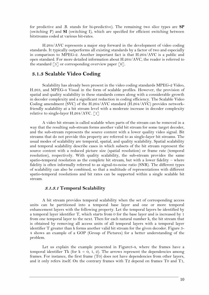
units can be partitioned into a temporal base layer and one or more temporal enhancement layers with the following property. Let the temporal layers be identified by a temporal layer identifier T, which starts from 0 for the base layer and is increased by 1 from one temporal layer to the next. Then for each natural number k, the bit stream that is obtained by removing all access units of all temporal layers with a temporal layer identifier T greater than k forms another valid bit stream for the given decoder. Figure 3-4 shows an example of a GOP (Group of Pictures) for a better understanding of the problem.

Let us explain the example presented in Figure3-4, where the frames have a temporal identifier Tk (for k = 0, 1, 2). The arrows represent the dependencies among frames. For instance, the first frame (T0) does not have dependencies from other layers, and it only refers itself. On the contrary frames with T2 depend on frames T0 and T1,

11

and they cannot be read without these frames. There is clearly a hierarchy between frames.

GOP

T0 T0T0T1 T1T2 T2 T2 T2

GOP

Figure 3-4: Hierarchical prediction structure for enabling temporal scalability.

3.1.3.2 Spatial Scalability

In the case of spatial scalability a new concept is introduced. Each layer

corresponds to a supported spatial resolution and is referred to by a spatial layer or dependency identifier D. The dependency identifier for the base layer is equal to 0, and it is increased by 1 from one spatial layer to the next. In each spatial layer, motion-compensated prediction and intra-prediction are employed as for single-layer coding. But in order to improve coding efficiency in comparison to simulcasting different spatial resolutions, additional so-called inter-layer prediction mechanisms are incorporated as illustrated in Figure 3-5 [1]. There are now 2 different layers: Base Layer (frames bellow) and Enhancement Layer (frames above). It can be seen that they have their own inter-dependencies and hierarchical frames, while the whole Enhancement is referenced by the Base Layer. There is not only a frame dependency, but also layer dependency.

GOP

T0 T0T0T1 T1T2 T2 T2 T2

GOP

Figure 3-5: Multilayer structure with additional inter-layer prediction for enabling

12

3.1.3.3 Quality Scalability

This last approach consists of pictures of the same size for a layer and the upper

layer in multilayer-coding, but with a higher fidelity to the original video stream in the higher encoded layer. It is also referred to as coarse-grain quality scalable coding (CGS). When utilizing inter-layer prediction for CGS in SVC, a refinement of texture information is typically achieved by re-quantizing the residual texture signal in the enhancement layer with a smaller quantization step size relative to that used for the preceding CGS layer.

The CGS concept only allows a few selected bit rates to be supported in a scalable

bit stream. In general, the number of supported rate points is identical to the number of layers. Switching between different CGS layers can only be done at defined points in the bit stream. Furthermore, the CGS concept becomes less efficient, when the relative rate difference between successive CGS layers gets smaller. Especially for increasing the flexibility of bit stream adaptation and error robustness, but also for improving the coding efficiency for bit streams that have to provide a variety of bit rates, a variation of the CGS approach, which is also referred to as medium-grain quality scalability (MGS), is included in the SVC design.[1]

In section 3.1 we have seen how video is compressed; we have explained some

advanced video coding technologies and how there are dependencies within the video stream that leads to a hierarchy of the data. That is, i.e., you cannot read layer 1,2 or 3 if you don´t have layer 0. Now I will talk about how this coded video stream is transmitted over an imperfect channel.

3.2 Video Transmission Advanced Video Coding (e.g. H.264, SVC… ) today is used in a wide range of

applications ranging from multimedia messaging, video telephony and video conferencing over mobile TV, wireless and Internet video streaming, to standard- and high-definition TV broadcasting. We will focus on a broadcasting video transmission channel (channels where one sender broadcasts to many receivers).

The transmission channel refers to the medium used to convey data from a sender

to a receiver. The problem is that these channels suffer from noise, distortion, interference, fading, etc…In all these cases, if we transmit data, e.g., encoded video stream, there is some probability that the received message will not be identical to the transmitted data.

We will model this imperfection into a Binary Erasure Channel (BEC), see Figure

3-6. In this model the transmitter sends a bit (a zero or a one), and the receiver either receives the bit or it receives a message that the bit was not received ("erased") and the erasure probabilities are unknown. Currently, the BEC is widely used to model the Internet.

13

Figure 3-6: Binary Erasure Channel Scheme.

Common methods for communicating over such channels employ a feedback

channel from receiver to sender that is used to control the retransmission of erased packets. For example, the receiver might send back messages that identify the missing packets, which are then retransmitted. Alternatively, the receiver might send back messages that acknowledge each received packet; the sender keeps track of which packets have been acknowledged and retransmits the others until all packets have been acknowledged [3].

The wastefulness of the simple retransmission protocols is especially evident in

the case of a broadcast channel with erasures. If every packet that is missed by one or more receivers has to be retransmitted, those retransmissions will be terribly redundant. Every receiver will have already received most of the retransmitted packets.

In Chapter 3.3 we will discuss codes for these broadcast erasure channels, where

every symbol is either received without error or erased. These codes have the property that they are rateless (the number of symbols transmitted is determined on the fly such that reliable communication is achieved, whatever the erasure statistics of the channel).

3.3 Forward Error Correction

Error correction coding is the means whereby errors which may be introduced into digital data as a result of transmission through a communication channel can be corrected based upon received data. Error detection coding is the means whereby errors can be detected based upon received information [7]. In order to do this, we add redundancy to the information, but instead of encoding one bit at a time, we add redundancy to blocks.

In the following subsection I will make a brief analysis of the current decoding algorithm used over the BEC, then I will describe the block codes, which are part of the Raptor Codes (section 3.3.3.2), and finally I will describe the rateless codes, on which this work is based.

14

3.3.1 Decoding Algorithms

3.3.1.1 Introduction

Decoding algorithm is a crucial part to create computationally efficient FEC

codes. The process of creating an efficient code starts by choosing an efficient algorithm that may or may not succeed. Later, the codes are designed around the algorithm, in such a way that the algorithm succeeds with high probability [8].

The iterative decoding algorithms, described in 3.3.1.2 are crucial on the study of

codes based on factor graphs. Gaussian elimination, described in section 3.3.1.3, is the original algorithm on which the current Raptor Code decoding algorithm is based. Gauss-Jordan elimination, described in section 3.3.1.4 is the algorithm used in our approach to optimize the rateless codes for SVC.

3.3.1.2 Message-Passing Algorithms

Message-Passing algorithms were developed to solve complicated global functions of

many variables, which can be visualized with a bipartite graph such as factor graph, which is a generalization of a Tanner graph. These algorithms are iterative and the reason for their name is because simple messages are passed locally among simple processors whose operations lead, after some time, to the solution of a global problem.

3.3.1.2.1 Sum-Product Algorithm

The sum-product is a generic message-passing algorithm and is the basic decoding

algorithm for codes on graphs. For finite cycle-free graphs, it is finite and exact. However, because all its operations are local, it may also be applied to graphs with cycles; then it becomes iterative and approximate, but in coding applications it often works very well. It has become the standard decoding algorithm for capacity-approaching codes, which are particular class of codes that can approach the Shannon limit quite closely (e.g., turbo codes, LDPC codes) [9].

The sum-product algorithm will involve messages of two types passing along the

edges in the factor graph: messages qn→m from variable nodes to factor nodes, and

messages rn→m from factor nodes to variable nodes. A message (of either type q or r) that

is sent along an edge connecting factor fm to variable 𝒳n is always a function of the

variable 𝒳n.

x3x2x1

rm n (xn) qn m (xn)

f2 f3 f4 f5f1

Figure 3-7: Sum-Product Algorithm. Factor Graph.

15

The algorithm operates by computing sums and products according to the following updating rules:

From variable to factor:

qn→m 𝒳n = 𝑟m'→n 𝒳n

𝑚 ′ ∈ℳ 𝑛 \𝑚

(3.1) From factor to variable:

rn→m Xn = fm(Xn) qn'→m 𝒳n'

n' ∈N m \n

Xm\n

(3.2)

A node that has only one edge connecting it to another node is called a leaf node.

A factor node that is a leaf node perpetually sends the message rn→m 𝒳n = fm(𝒳n) to its

one neighbor 𝒳n (Figure 3.8a). A variable node that is a leaf node perpetually sends the

message qn→m 𝒳n = 1 (Figure 3.8b).The algorithm terminates once two messages have been passed over every edge, one in each direction. For more information I would like to refer the reader to [10] and [11].

xn

fm

rm n (xn) = fm (xn)

xn

fm

qn m (xn) = 1

Figure 3-8a: Factor leaf node Figure 3-7b: Variable leaf node

There are many variants and applications of the sum-product algorithm. The most straight-forward application is to a posteriori probability (APP) decoding. In the field of statistical inference, it becomes the even more widely known “belief propagation” (BP) algorithm. For Gaussian state-space models, it becomes the Kalman smoother. There is also a “min-sum” or maximum-likelihood sequence detection (MLSD) version of the sum-product algorithm. When applied to a trellis, the min-sum algorithm gives the same result as the Viterbi algorithm [11].

3.3.1.2.2 Belief Propagation

This decoding algorithm, which is known under the names of “belief propagation

decoder,” “peeling decoder,” or “greedy decoder,” it is best described in terms of the “decoding graph” corresponding to the collected output symbols. There is simple erasure recovery algorithm described in [9], which performs the following steps until either no output symbols of degree one are present in the graph, or until all the input symbols have

16

been recovered. At each step of the algorithm, the decoder identifies an output symbol of degree one. If none exists, and not all the input symbols have been recovered, the algorithm reports a decoding failure. Otherwise, the value of the output symbol of degree one recovers the value of its unique neighbor among the input symbols. Once this input symbol value is recovered, its value is added (modulo 2) to the values of all the neighboring output symbols, and the input symbols and all edges emanating from it are removed from the graph. An example is given in Figure 3-9.

+ + + + + + + +

1 0 1 1

1

+ + + +

1 1 1 0

1

+ + + +

1 0

+ + + +

1 1 1 0

1 0

+ + + +

1 1 1 0

1 0 1

Figure 3-9: Belief Propagation Algorithm.

3.3.1.2.3 The min-sum algorithm and ML decoding

With minor modifications the sum-product algorithm may be used to perform a

variant of maximum-likelihood (ML) sequence decoding rather than APP decoding. The sum-product algorithm can be turned into a max-product algorithm by replacing every “sum” by “max”. In practice, the max-product algorithm is most often carried out in the negative log likelihood domain, where max and product become “min” and “sum”. The min-sum algorithm is also known as the Viterbi algorithm [10].

3.3.1.3 Gaussian Elimination.

Gaussian elimination is a method for solving matrix equations of the form Ax = b,

where A is a kxk matrix, b is a kx1 vector and x is the a kx1 vector of variables. The method brings the augmented matrix,

𝑎11 𝑎12 ⋯ 𝑎1𝑘 𝑎21 𝑎22 ⋯ 𝑎2𝑘

⋮ ⋮ ⋱ ⋮ 𝑎𝑘1 𝑎𝑘2 ⋯ 𝑎𝑘𝑘

𝑏1𝑏2⋮

𝑏𝑘

(3.3)

17

into to and to an upper triangular form, by performing elementary row operations. The upper triangle form solves one of the equations for one variable (in terms of all the others).

𝑎′11 𝑎′12 ⋯ 𝑎′1𝑘 0 𝑎′22 ⋯ 𝑎′2𝑘

⋮ ⋮ ⋱ ⋮ 0 0 ⋯ 𝑎′𝑘𝑘

𝑏′1𝑏′2⋮

𝑏′𝑘

(3.4)

Then, resolves the other equations doing back substitution.

In the case of the erasure channel, ML decoding of linear codes is equivalent to

solving systems of linear equations. This task can be done in polynomial time using Gaussian elimination or Gauss. However, Gaussian elimination is not fast enough, especially when the length of the code is long.

3.3.1.4 Gauss-Jordan Elimination.

Gauss–Jordan elimination is a version of Gaussian elimination that brings a Amxk

matrix to reduced row echelon form. A matrix is said to be in reduced echelon form if:

(1) Any rows consisting entirely of zeros are grouped at the bottom of the matrix.

(2) The first nonzero element of any row is 1. This element is called a leading 1.

(3) The leading 1 of each row after the first is positioned to the right of the leading 1 of the previous row.

(4) If a column contains a leading 1, then all other elements in that column are 0.

By using elementary row operations (row exchange, row scaling and row replacement) we could bring the matrix to this form the reduced echelon form. This is done by first creating leading 1s, then ensuring that columns containing leading 1s have only 0s above and below the leading 1, column by column starting with the first column. The matrix in reduced echelon form will either give the solution or demonstrate that there is no unique solution. The process (3.5), shows an example where all the variables of matrix (3.3) cab be resolved.

1 𝑎′12 ⋯ 𝑎′1𝑘 0 𝑎′22 ⋯ 𝑎′2𝑘

⋮ ⋮ ⋱ ⋮ 0 𝑎′𝑘2 ⋯ 𝑎′𝑘𝑘

𝑏′1𝑏′2⋮

𝑏′𝑘

->

1 0 ⋯ 𝑎′1𝑘 0 1 ⋯ 𝑎′2𝑘

⋮ ⋮ ⋱ ⋮ 0 0 ⋯ 𝑎′𝑘𝑘

𝑏′1𝑏′2⋮

𝑏′𝑘

-> … ->

1 0 ⋯ 0 0 1 ⋯ 0 ⋮ ⋮ ⋱ ⋮ 0 0 ⋯ 1

𝑏′1𝑏′2⋮

𝑏′𝑘

(3.5)

Suppose the system has m equations with k unknowns, and k > m. Amxk has r ≤ m

leading 1s, so at least k-m of the variables can take any value. This shows that there are

18

many solutions. Gauss–Jordan elimination is considerably less efficient than Gaussian elimination with back substitution when solving a system of linear equations. However, it works with mxk matrices and can bring the maximum number of solutions for a system of linear equation.

Gauss-Jordan elimination gives the key to partially resolve sparse matrices, that is

to decode part of the source symbols if not all of them are decodable. This feature will be essential for the development of our work.

3.3.2 Linear Block Codes

3.3.2.1 Introduction

A block code is a rule for converting a sequence of source bits „s‟, of length K, say,

into a transmitted sequence „t‟ of length N bits. To add redundancy, we make N greater than K. In a linear block code, the extra N - K bits are linear functions of the original K bits; these extra bits are called parity-check bits.

t = GTs (3.6) Where G is the generator matrix of the code

GT =

1 0 0 0 0 1 0 00 0 1 00 0 0 11 1 1 10 1 1 11 0 1 1

(3.7)

and the encoding operation use modulo-2 arithmetic (1+1=0, 0+1=1, 1+0=1, 1+1=0). The generator matrix could be seen in its standard form

G = Ik | P (3.8) and then the parity-check matrix, H, can be calculated as

H = [ PT| In-k ] (3.9) The syndrome satisfies z= Ht and for any valid codeword „t‟, it will be zero [12].

19

3.3.2.2 Hamming Codes

The Hamming Codes were named after its inventor, Richard Hamming and

published in 1950. Hamming codes can detect up to two simultaneous bit errors, and correct single-bit errors; thus, reliable communication is possible when the Hamming distance between the transmitted and received bit patterns is less than or equal to one. By contrast, the simple parity code cannot correct errors, and can only detect an odd number

of errors. For each integer m > 2 there is a code with m parity bits and 2m − m − 1 data bits. The parity-check matrix of a Hamming code is constructed by listing all columns of length m that are pairwise independent. For more information I would like to refer the reader to [13].

3.3.2.3 LDPC Codes

Low-Density Parity-Check (LDPC) Codes have recently been recognized as one of

the most powerful forward-error-correcting codes, which assure performance very close to the Shannon limit capacity. First proposed by Gallager in 1962 [14], they were forgotten by the coding world as they showed a decoding complexity too high for the computation capabilities at that time. Recently, in 1995, Mackay and Neal [15] rediscovered Gallager´s codes, and opened the road to much further research.

The parity-check matrix, H, was defined in a non-systematic form; each column of

H had a small weight (e.g. 3) and the weight per row was also uniform; the matrix H was constructed at random, subject to these constraints.

The matrix, H, can also be seen as a Tanner Graph which is sparse bipartite graph

used to specify constraints or a set of linear equations [16].

x2 x3x1 x4 x5 x6

+ + +

Figure 3-10: LDPC Code

The bits of a valid message, when placed on the circles on the top of the graph,

satisfy the graphical constraints. Specifically, all lines connecting to a variable node (x1,

x2…xn) have the same value, and all values connecting to a factor node (box with a '+' sign) must sum, modulo two, to zero (in other words, they must sum to an even number).

The crucial innovation was Gallager‟s introduction of iterative decoding

algorithms (or message-passing decoders), described in section 3.3.1.2.

20

3.3.3 Rateless Erasure Codes

Rateless Erasure Codes, also known as Fountain Codes, are a novel and innovative class of codes designed for transmission of data over time varying and unknown erasure channels. They were first mentioned without an explicit construction in [17]. The idea is to be able to generate a potentially limitless sequence of encoding symbols (y1,y2,…) from

a given set of source k symbols (x1,x2,…xk). A reliable decoding algorithm for a rateless

code is one which can re-cover the original k input symbols from any set of N output

symbols with error probability at most inversely polynomial in k. The ratio N/k is called

the overhead.

The rateless codes can also be seen as a set of equations, where the output symbols would represent linear combination of the input symbols.

A ·

𝑥1...

𝑥𝑘

=

𝑦1𝑦2

.

.

.𝑦𝑁

(3.10)

Where „A‟ is a matrix that represents the relationship between the input symbols

and the collected output symbols and it is associated with the factor graph. Each output symbol would be generated by adding (modulo 2) the corresponding source symbols.

In effect, all decoding methods for rateless codes try to solve this system of equations, either implicitly or explicitly. The task of the code designer is to design the rateless code in such a way that a particular (low-complexity) decoding algorithm performs very well.

3.3.3.1 LT Codes

LT Codes were the first efficient realization of Rateless codes. They were invented

by Luby in 1998 and exhibit good overhead and error probability properties [18]. Each encoded packet yn is produced from the source symbols (x1,x2,…xk) as follows:

Randomly choose the degree dn of the packet from a degree distribution Ω(d); the

appropriate choice of Ω will be discussed later.

Choose, uniformly at random, dn distinct input packets, and set yn equal to the bitwise sum, modulo 2 of those dn packets. This sum can be done by successively

exclusive-or-ing the packets together. This encoding operation defines a graph connecting encoded packets to source

packets. If the mean degree of d is significantly smaller than k then the graph is sparse. We can think of the resulting code as an irregular low-density generator-matrix code. The decoder needs to know the degree of each packet that is received, and which source packets is connected to in the graph.

21

x1 x2 x3 x4 x5 x6

y1 y2 y3 y4 y5 y6 y7

Y1 = x3 + x5 + x6

Y2 = x1 + x2 + x3

Y3 = x1 + x4

Y4 = x3

Y5 = x1 + x6

Y6 = x3 + x6

Y7 = x2 + x4 + x5 + x6

Figure 3-11: LT Code. Equations and factor graph

The random behaviour of the LT process is completely determined by the degree

distribution Ω(d),the number of encoding symbols K, and the number of input symbols k. As far as the design of the LT decoder, Gaussian elimination is computationally expensive for dense codes like random LT-codes. For properly designed LT-codes, the BP decoder provides a much more efficient decoder. For random LT-codes the BP decoder fails miserably even when the number of collected output symbols is very large. Thus, the design of the degree distribution must be dramatically different from the random distribution to guarantee the success of the BP decoder [9].

The first approach of degree distribution from Luby is called Ideal Soliton

distribution (Figure 3-12). This degree distribution theoretically minimizes the expected number of redundant code that will be sent before the decoding process can be completed.

The Ideal Soliton distribution is ρ(1), . . . , ρ(k), where

ρ(1) = 1/k

For all i = 2,…., k, ρ(i ) = 1/ i (i - 1) (3.11)

Figure 3-12: Ideal Soliton Distribution

22

This distribution is quite fragile, because the low probability of nodes with degree one, which is needed to start the BP algorithm .In fact it is useless in practice, but it does give insight into a Robust distribution (Figure 3-13). The Robust Soliton distribution is µ(.)

defined as follows. Let R= c∙ln(k/δ) 𝑘 for some suitable constant c>0. Define,

τ (i ) = R/ik for i=1,….,k/R-1

Rln(R/δ)/k for i=k/R

0 for i=k/R+1,….,k

(3.12)

Add the Ideal Soliton distribution ρ(.) to τ(.) and normalize to obtain µ(.):

β = 𝜌 i + τ i 𝑘𝑖=1

For all i=1,….,k, µ(i )= (𝜌 i + τ i )/𝛽 (3.13)

Figure 3-13: Robust Soliton Distribution, note the spike.

The Robust Soliton distribution produces more packets of degree ones and more packets of high degree, see Figure 3-13, that assures to have every source symbol connected.

3.3.3.2 Raptor Codes

The complexity of encoding and decoding an LT code is directly related to the

degree distribution. The smaller the average degree is, the less the number of XORs involved in calculating each encoded symbol and the simpler the encoding and decoding processing. At the same time, the degree distribution must allow the decoding process to fully recover the entire source block with a number of received encoded symbols only slightly larger than the total number of source symbols. Well-performing degree distributions for LT codes have been determined, but the resulting complexity is not linear with respect to the number of source symbols.

An extension of LT-codes, Raptor codes are a class of erasure rateless codes with

constant encoding and linear decoding cost [19]. In order to achieve linear complexity,

23

Raptor encodes in two stages: first, a low-complexity pre-coding algorithm is applied to the input block of source symbols to create a pre-coded block, and then an LT code is applied on the pre-coded block to generate an unlimited number of encoded symbols from the pre-coded block.

Precoding

LT-coding

Redundant nodes

Figure 3-14: Raptor Code. Diagram

The key idea of Raptor Coding is to relax the condition that all input symbols need to be recovered. Thus, it is possible to use a simpler degree distribution that does not recover all the symbols but makes the decoding process faster.

x1 x2 x3 x4 x5 x6

y1 y2 y3 y4 y5 y6 y7

Y1 = x1

Y2 = x1 + x5

Y3 = x1 + x3 + x4

Y4 = x1 + x3 + x4 + x6

Y5 = x4 + z2

Y6 = x5 + z2

Y7 = x4 + x5 + x6 + z1

0 = x1 + x3 + x4 + x6 + z1

0 = x1 + x2 + x4 + x5 + x6 + z2

z1 z2

x1 x2 x3 x4 x5 x6

y1 y2 y3 y4 y5 y6 y7

z1 z2

0 0

Figure 3-15: Raptor Code. . Equations and factor graph

The output degree distribution Ωr(i), is similar to the Soliton distribution, but it has been modified by capping it at some maximum degree D, and giving it an appropriate weight for output symbols of degree one.

Ωr (i ) =

𝜌

1+ 𝜌 for i=1

1

𝑖 𝑖−1 (1+𝜌) for i=2,….,D

1

𝐷(1+𝜌) for i=D+1

(3.14)

Where D = 4(1 + ε)ε and ρ = ε/2 + ε/2 2.

24

4 Approach

4.1 Related Work

We found 3 scientific papers related to rateless codes with unequal protection which can be used for application where a portion of data may need more protection than the rest of data. This concept could also be applied to video streaming, as seen in section 3.1.

In the following sections we will make a brief analysis of these papers.

4.1.1 Unequal-Protected LT Code for layered video streaming

The main idea of the paper [20] is to control the Degree distribution and to be

able to control each symbol decoding probability. In the decoding process, every symbol is decoded through one or more decoding paths. It was observed that the original symbols with more decoding paths are easier to be decoded than others, and symbols with shorter decoding paths can be decoded more quickly than others.

The traditional coding graph of LT code is randomly generated. This means the decoding probability and decoding priority of a symbol is uncertain. It was proposed a hierarchical coding graph, where the circular nodes and square nodes denote original packets and encoded packets, respectively.

Figure 4-1: Hierarchal coding graph. From [20]

There are two important features in the proposed structure. First, the decoding process starts from leaves, so packets toward leaves can have higher decoding priority on average. Secondly, packets near leaves have more short decoding paths, so they also have higher decoding probability on average. Therefore, it was proposed a randomized algorithm to generate a coding graph of Unequal-Protected LT Code.

Although their results were encouraging they were not precise. The coding algorithm and the mathematical analysis were not clear enough to reproduce the system

25

and check the results. Moreover the maximum degree is 3, which doesn‟t correspond to the currently LT Code.

4.1.2 Prioritized LT Codes

In this scientific paper [21], it is proposed a new scheme which modifies the conventional LT encoder to send high priority data as a degree 1 and 2. Since these degrees critically affect the decoding performance, high priority data can be quickly resolved and very likely recovered before the BP decoding algorithm stops.

The key ideas behind their scheme are the following: the encoder imposes a

constraint on the degree 1 and degree 2 encoded bits. All degree 1 encoded bits are selected from a high priority data group. This is because, in decoding LT codes, a degree 1 encoded bits are necessary for a decoder to initiate the decoding process. Degree 2 encoded bits can be directly decodable from the degree 1 encoded bit. Degree 2 encoded

bits should include a number, Ω, of high priority bits to make use of decoded degree 1

high priority bits. A value around Ω ~ h/2 seems to be a reasonable choice, since it is the number of degree 2 required for decoding packet size h so that it can decode high priority data first.

The proposed idea was intuitive and it could be easily reproduced, with

encouraging results. However, the good performance of the code is based on the Robust Soliton distribution, which has a continuous range of degrees and it doesn‟t make a clear contribution on other less complex degree distribution (for example Raptor Code‟s degree distributions). The idea is based on characteristics of the iterative belief propagation algorithm, and it is not clear that it could be extended to other decoding methods.

4.1.3 Rateless Codes with Unequal Error Protection

In [22], it is proposed a modification in the structure of rateless codes to provide unequal error protection (UEP) and unequal recovery time (URT) properties. This means that given a target bit error rate, different parts of information bits can be decoded after receiving different amounts of encoded bits.

In the LT encoding scheme all the input nodes have the same probability of being

selected in forming each output node. Consequently, the code provides Equal Error Protection for all data. In their proposed scheme, the neighbours of a encoded packets are selected non-uniformly at random. They partition the n variable nodes into r sets s1, s2 . . sr and with a probability pj (n) that an edge is connected to a particular variable node in sj, for j = 1, . . . , r (see Figure 4-2).

26

Figure 4-2: Non-uniform probability distribution function for selecting an input symbol by an edge. From [22]

They analyzed the performance of the proposed structure asymptotically. To investigate the recovery probability of an input symbol in a generalized rateless code, it is used the technique called And-Or tree analysis [23] and it is then generalized to fit the belief propagation algorithm. They showed that UEP-rateless codes can provide very low error rates for more important bits with only a subtle loss on the performance of less important bits.

They focused afterwards on finite-length rateless codes and derived upper and

lower bounds on the maximum-likelihood decoding bit error rates of EEP- and UEP-rateless codes.

4.2 Progressive FEC for video

After the small research made above, we have noticed that there are not many approaches on this topic. There is not even a standard or a research topic. We have also noticed that all the approaches are focused on LT Codes and there are only theoretically tackled. Hence we decided to implement our own rateless code which we will call “Progressive FEC for video”. We will make a practical analysis of this rateless code, implementing a system with coder, simulated erasure channel and decoder.

The goal is to design a rateless code, which produces a single packetstream that

unequally protects the multilayer source code. It will give more protection to more important layers and will be able to decode them progressively, starting form the most important layers. It will adapt to a variable number of layers and it will be systematic (the first K encoded symbols are the source symbols).

The work is based on the latest erasure rateless codes: LT Codes and Raptor

Codes. Forward error correction codes are usually characterized by a rate and a distance. These parameters help one ensure correct data transmission in a particular channel setting. However, in some cases, the channel characteristics are not known, and yet one would like to achieve data transmission without sending excessive amounts of data, while maintaining efficient encoding and decoding. The rateless erasure codes achieve these goals and are used to transmit data packets over the internet, that is, originally designed for reliable transmission of data over an erasure channel with unknown erasure probability (BEC).

From now on we will suppose a multimedia broadcast scenario following these

properties:

27

The source data is produced following the Scalable Video Coding.

The source data is then encoded using the Progressive FEC for video which produces one rateless stream of packets.

The sender transmits packets one at a time with a fix packet rate to every device within the broadcast domain.

The packets will be transmitted over a Binary Erasure Channel, and packets will be randomly dropped according to packet erasure rate.

Each device will receive packets over the channel until the information can be reconstructed with no termination signal.

Depending on the amount of received packets each device will be unable to decode the source data or progressively decode base layer, which provides basic quality, and successive layers which will refine the quality incrementally.

The design and development of this approach will be in the next chapter

described.

28

5 Design and Development

We started with a design of an LT Code system, because they were the first practical rateless codes and there are easier to implement. The key of the optimization of rateless codes for SVC is the LT Code distribution, and it could be then extended to Raptor Codes. The next step was to study the Raptor Codes, which really have good performance and constant encoding and linear decoding cost. Again, we implemented a non-systematic Raptor Code because it is easier to study, but afterwards it is necessary to implement a Systematic Raptor Code version, since it dramatically reduces the complexity when low packet drop rates allow most packets to be received uncoded.

5.1 LT Code Optimization

5.1.1 Design To begin with, we implemented and simulated a complete LT Code system, in

order to analyze and study the practical performance of it, and how the degree distribution affects the individual decoding probability and the general performance. The degree distribution is the sole component responsible for the efficiency of the LT codes, and it can be the key on distributing decoding probabilities. In general, the optimization of the degree distribution is not a trivial problem.

The LT encoder, section 5.1.1.1, has been based on Standardized Raptor Codes

IETF [24] and for the decoding process we have implemented a LT Decoder based on the Belief propagation algorithm explained in 3.3.1.2.2. After implementing the system we used different degree distributions to see how it affects the decoding probability of the source symbols (Section 5.1.1.2 and 5.2.1).

5.1.1.1 LT encoder

The LT encoder generates N>K repair symbols, where K is the number of source

symbols. Each repair symbol is created by applying the function,

C'[i] = LTEnc[K, (C[0],..., C[K-1]), (d[i], a[i], b[i])],

for all i, 0 <= i < N (5.1)

where C[0], C[1],..., C[K-1] are the source symbols and d[i], a[i], b[i] that we will call the triple associated with the repair symbol.

29

The encoding symbol generator produces a single encoding symbol as output,

according to the following algorithm:

While (b >= K) do b = (b + a) % K'

Let result = C[b]. For j = 1,...,min(d-1,K-1) do b = (b + a) % K' While (b >= K) do b = (b + a) %K' result = result ^ C[b]

Return result (5.2)

K' is the smallest prime that is greater than or equal to K, % denotes modulo and ^ denotes, for equal-length bit strings the bitwise exclusive-or.

The source triples, defined in equation 5.1, are determined using the Triple generator,

(d, a, b) = Trip[K,X] (5.3)

The Encoding Symbol ID (ESI), X, values from 0 to N-1 identify the repair symbols of a source block in sequential order. Let J(K) be the systematic index associated with K, as defined as defined in Section 5.7 of [24] and Q = 65521, the largest prime smaller than 216. The output of the triple generator is a triple, (d, a, b) determined as follows:

A = (53591 + J(K)*997) % Q B = 10267*(J(K)+1) % Q Y = (B + X*A) % Q v = Rand[Y, 0, 220] d = Deg[v] a = 1 + Rand[Y, 1, K'-1]

b = Rand[Y, 2, K' ] (5.4)

The random number generator Rand[X, i, m] is defined as follows, where X is a

non-negative integer, i is a non-negative integer, and m is a positive integer and the value

30

produced is an integer between 0 and m-1. Let V0 and V1 be arrays of 256 entries each, where each entry is a 4-byte unsigned integer. These arrays are provided in Section 5.6 of [24]. Then,

Rand[X, i, m] = (V0[(X + i) % 256] ^ V1[(floor(X/256)+ i) % 256])% m (5.5)

The degree generator Deg[v] is defined as follows, where v is an integer that is at least 0 and less than 220= 1048576. Then you make table distributed the possible degrees from 0 to 220, in accordance to its probabilities. In table (5.6), find the index j such that f[j-1] <= v < f[j]. Then, Deg[v] = d[j] and d = Deg[v].

+--------+---------- -+------+ | Index j | f[j] | d[j] | +-------- +---------- +------ + | 0 | 0 | --- | | 1 | 10241 | 1 | | 2 | 491582 | 2 | | 3 | 712794 | 3 | | 4 | 831695 | 4 | | 5 | 948446 | 10 | | 6 | 1032189| 11 | | 7 | 1048576| 40 |

+-- -------+----------+-------+ (5.6)

5.1.1.2 LT degree distribution

The analysis of the LT Code started with three different degree distributions:

from the standardized systematic Raptor Code [24], from the original Raptor Code [19] and from the research paper “Optimizing the Degree Distribution of LT Codes with an Importance Sampling Approach” [25], which we will call “Optimized LT Distribution”. The degrees, d[j], and its probabilities, p[j], are shown below in (5.7), (5.8), (5.9).

d[j] = [0,1,2,3,4,10,11,40]; p[j] = [0,0.0098,0.4590,0.2110,0.1134,0.1113,0.0799,0.0156];

% Systematic Raptor Distribution (5.7) d[j] = [0,1,2,3,4,5,8,9,19,64,66]; p[j] = [0,0.0080,0.4936,0.1662,0.0726,0.0826,0.0561,0.0372,0.0556,

0.0250,0.0031];

% Original Raptor Distribution (5.8) d[j] = [0,1,2,4,8,16,32,64]; p[j] = [0,0.1900,0.3400,0.2700,0.1300,0.0300,0.0100,0.0300];

% Optimized LT Distribution (5.9)

The three degree distributions are represented in Figure 5-1, Figure 5-2 and Figure 5-3.

31

Figure 5-1: Systematic Raptor Degree Distribution

Figure 5-2: Original Raptor Degree Distribution

Figure 5-3: Optimized LT Degree Distribution

32

5.1.2 Testing and Results

For the study of the LT Code we have empirically calculated the probabilities. To that end we simulated a complete LT Code system, represented in Figure 5-4. We created randomly the source symbols, we made the LT encoding, we simulated an erasure channel, we decoded the received symbols and we read the decoding probability form each source symbol. The erasure channel was emulated by dropping randomly packets according to different erasure rates. In our case the erasure rates will be represented as Packet Receiving Rate (PRR), which is the relation between the number of received packets and the number of source symbols. The simulation was repeated several times for each packet receiving rate and each time the decoding success of each symbol was recorded.

Source

Generator

LT

EncoderBEC

Packetloss

LT

Decoder

Decoding

Probabilty

Figure 5-4 : LT Code System: Block Diagram.

We used a number of 1024 symbols because it is a reasonable size of information in

terms of video coding. The information was also divided in two parts. The first part was called Base Layer in reference to the Scalable Video Coding and it would give the basic video quality. The Enhancement layer would give extra quality if both layers are received. The proportion of them (Base Layer (40%) and Enhancement Layer (60%)) tried also to be realistic with real Scalable Video Coding stream rates.

The system was implemented and simulated with Matlab and following the next characteristics:

1024 source symbols. LT encoding.

1536 encoded symbols (0.5 overhead). 3 different Degree Distributions: Systematic Raptor, Original Raptor and

Optimized LT Code distribution. Decoding with Belief Propagation.

25 different packet receiving rates: PRR=[ 1.5: -0.05 : 0.3]. The simulation was run 1000 times for each packet receiving rate and for each

degree distribution. Recording of each test. Two Layers. Base Layer (40%) and Enhancement Layer (60%).

33

The aim of this analysis is to know which symbols have better decoding probability.

To that end the Probability Density Function (PDF) can help us telling how the decoding probability is distributed over all the symbols. In our case we will use the normal distribution, which will tell us easily which is the mean decoding value, how many symbols are around this value and how do the probabilities spread over this value. For instance Figure 5-5 show us a mean value of 65% of decoding probability, but very spread probabilities that goes approximately from 50% to 80% of decoding probability.

Figure 5-5: Probability Density Function of LT Code with Systematic Raptor Degree Distribution. 111% Packet receiving rate.

It is also interesting to see how the function develops over the packet receiving

rate. As shown in Figure 5-6, at the beginning practically every symbol has 100% of probability to be decoded. It seems that just a few symbols cannot be decoded. When it reaches 121% of packet receiving rate, it spreads rapidly, and the curve gets wider. This feature would help selecting symbols with good and bad probability, but by 111% packet receiving rate, which is quite lot overhead, there are no symbols with good decoding probability.

34

Figure 5-6: Progress of Probability Density Function over different packet receiving rate.

The next step is to find out which are the symbols with better decoding probability, so we developed our own function to read this information from the tests. The 40% symbols with best decoding probability were treated as Base Layer and the 60% left as Enhancement Layer. Then we simulated the probability of a whole layer to be decoded, that is, every symbol of each layer decoded at the same time.

Figure 5-7, Figure 5-8 and Figure 5-9 represent the layer decoding probability of

the Base layer, Enhancement layer over the packet receiving rate and for three different degree distributions. It is also represented the decoding probability of all the symbols at the same time, as if there was only one layer. As shown in the figures, the Base Layer has better performance than the Enhancement Layer. The symbols with worse decoding probability are set in the Enhancement Layer and will define the performance of this layer and as a result of it the performance of the 1 layer version (green line).

We also checked that the Enhancement Layer has only a few source symbols which fail regularly by the decoding and this fact coincides with observation made from the density function (Figure 5-9). If we make the supposition of the later recovery from these symbols by the pre-code, it is verified that the two layers match up. Nevertheless the general performance is not optimal, needing a huge overhead (more than 20%). That is because of the belief propagation decoding, which fails each time it doesn´t find a degree 1 node.

35

Figure 5-7: LT Code: Layer Decoding Probability with the systematic Raptor code distribution.

Figure 5-8: LT Code: Layer Decoding Probability with the original Raptor code distribution.

36

Figure 5-9: LT Code: Layer Decoding Probability with the Optimized LT Code distribution.

It has been proved that the BP decoder fails miserably for other LT distributions even when the number of collected output symbols is very large. However there is a gain in layered LT Code. Some symbols are more likely to be decoded than others. After these first conclusions we may continue with a non-systematic Raptor Code system.

37

5.2 Non-Systematic Raptor Code Optimization

5.2.1 Introduction

We have focused our work on Raptor Codes because they are a class of rateless codes with constant encoding and linear decoding cost and it is possible to use a simpler degree distribution that does not recover all the symbols but makes the decoding process faster. It has been based on Standard Standardized Raptor Codes IETF[24]. The code was designed with a variety of requirements in mind: it had to work well for numbers of input symbols between 500 and 8196, it had to be systematic, and it had to have a simple description.

The pre-code step has to stages: the first stage of the pre-code uses a regular

LDPC code, described in 3.3.2.3, while the second stage uses a code that is somewhat similar to the Hamming code, described in 3.3.2.2. Once the intermediate symbols have been generated, repair symbols are produced as described on section 5.1.1.1, but using as input the L intermediate symbols produced by the pre-code. Then,

C'[i] = LTEnc[K, (C[0],..., C[L-1]), (d[i], a[i], b[i])],

for all i, 0 <= i < N (5.10)

where C[0],..., C[L-1] are the intermediate symbols.

We will describe, in section 5.2.2.1, how the standard pre-code is created and in section 5.2.2.2 how the standard generator matrix is built. We will also make a brief description of the standard decoder and why we will use the Gauss-Jordan elimination decoder in section 5.2.2.3. Finally we will explain how we modified the matrix generator, section 5.2.2.4, we will test the new modification and see the results in section 5.23.

5.2.2 Design

5.2.2.1 Pre-Code

The pre-coding relationships amongst the L intermediate symbols are defined by

expressing the last L-K intermediate symbols in terms of the first K intermediate symbols. To begin with, let us define the variables that are used in the following algorithms. Let

- X be the smallest positive integer such that X*(X-1) >= 2*K.

- S be the smallest prime integer such that S >= ceil(0.01*K) + X

- H be the smallest integer such that choose(H,ceil(H/2)) >= K + S

- H' = ceil(H/2)

- L = K+S+H

38

The S LDPC symbols are defined to be the values of C[K],...,C[K+S-1] at the end of the following process:

For i = 0,...,K-1 do a = 1 + (floor(i/S) % (S-1)) b = i % S C[K + b] = C[K + b] ^ C[i] b = (b + a) % S C[K + b] = C[K + b] ^ C[i] b = (b + a) % S

C[K + b] = C[K + b] ^ C[i] (5.11)

The H Half symbols are defined as follows. Let

- g[i] be the Gray sequence, in which each element differs from the previous one in a single bit position: g[i] = i ^ (floor(i/2)) for all positive integers i.

- m[k] denote the subsequence of g[.] whose elements have exactly k non-zero bits in their binary representation.

- m[j,k] denote the jth element of the sequence m[k], where j=0, 1, 2, ...

Then, the Half symbols are defined as the values of C[K+S],...,C[L-1] after the

following process:

For h = 0,...,H-1 do For j = 0,...,K+S-1 do

If bit h of m[j,H'] is equal to 1 then C[h+K+S] = C[h+K+S] ^C[j] (5.12)

5.2.2.2 Generator Matrix: Standard Version.

The generator matrix, A, for a code that generates N output symbols from L input symbols is an MxL matrix over GF(2), where M=N+S+H.

Let

- C denote the column vector of the L intermediate symbols, C[0],C[1],..., C[L-1].

39

- D denote the column vector consisting of S+H zero symbols followed by the N repair symbols C'[0], C'[1], ..., C'[N-1].

Then the constraints of 5.111 and 5.221 define the A matrix such that:

A*C = D (5.13) The equation is depicted in Figure 5-10 below:

As

AH

0

AE

S

O

U

R

C

E

S

Y

M

B

O

L

S

H

A

L

F

L

D

P

C

R

E

P

A

I

R

S

Y

M

B

O

L

S

K S H

S

H

N

0

0

Figure 5-10: Non-systematic Raptor. Encoding Equation A*C=D

5.2.2.3 Raptor Decoding: Inactivation and Gauss-Jordan Decoding.

The aim of the Raptor decoder is to obtain the intermediate symbols, where you can

directly read the source symbols. That is, to solve C from the equation 5.13.

In the standard version they propose an algorithm called “Inactivation Decoder” [26]. This decoder is in fact an ML decoder; the code can be designed in such a way that this decoder works with minimal computational overhead. Therefore, the algorithm is nothing but an alternative way of implementing standard Gaussian elimination. The basic idea of inactivation decoding is to declare an input symbol as inactivated whenever the greedy algorithm fails to find an output symbol of weight 1. As far as the algorithm is concerned, the inactivated symbol is treated as decoded, and the decoding process continues. The values of the inactivated input symbols are recovered at the end using Gaussian elimination on a matrix in which the number of rows and columns are roughly equal to the number of inactivations.

The inactivation decoder can solve, when possible, all the variables of the equation,

but it is not able to solve some variables if not all of them are resolvable. That is, it cannot solve individual symbols. According to the multilayer concept, this would be desirable in order to be able to decode separately different layers. In these work it is proposed to use the “Gauss-Jordan elimination” (described in 3.314) which has this

40

capacity. Furthermore, it is able to solve some variables having fewer equations than variables. That would mean to have an A Matrix with fewer rows than columns.

5.2.2.4 Separate Pre-coding and LT Code improvement

The main goal is to improve the LT Code, by controlling node connections, giving

different decoding probabilities to the source symbols depending on the layer where they are. It will be also necessary to have separate pre-codings for each layer, so they could correct independently the erasure symbols. Following the same schedule from above, we propose the scheme in figure 5-11, which is can be extended to a variable number of layers.

AS1

AH1

0

AE

S1

R

E

P

A

I

R

S

Y

M

B

O

L

S

S1

H1

N

0

0

AS2

AH2

0S2

H20

0

K1 S1 H1 K2 S2 H2

H1

S2

H2

K1

K2

Figure 5-11: Non-systematic Raptor. 2-layer Generator Matrix.

5.2.3 Testing and Results

We simulated a Raptor Code system with a random Source Symbol generator, Raptor Encoder, Binary Erasure Channel, Raptor Decoder, Decoding probability reader (Figure 5-12). We record each test and read the probability of each source symbol to be decoded.

41

Source

Generator

Raptor

EncoderBEC

Packetloss

Raptor

Decoder

Decoding

Probabilty

Figure 5-12: Raptor Code System: Block Diagram.

The system was implemented and simulated with Matlab and following the next characteristics:

1024 source symbols. Raptor encoding with the 2 layer Generator Matrix (Figure 5-11).

3 different Degree Distributions for the LT part: Systematic Raptor [24], Original Raptor [19] and modified as in [21].

Decoding with Gauss-Jordan Elimination. 23 different packet receiving rates: PRR=[ 1.1: -0.05 : 0].

The simulation was run 1000 times for each packet receiving rate and for each test.

Recording of each test.

Two Layers. Base Layer (40%) and Enhancement Layer (60%).

The Base Layer represented the 40% first Source symbols (symbols with blue lines)

and Enhancement layer (symbols with green lines) the rest of the Source symbols. In order to have a clearer vision from the graphics, we represented 10 black lines which delimit a number of 10% from the Source symbols.

Figure 5-13 represents the symbol decoding probability from the Standard Raptor Code [24], but using this time the gauss-Jordan decoder. Clearly, almost all the source symbols have the same decoding probability. Consequently, the code provides equal encoding probability, but with 5% it is possible to decode every single symbol.

42

Figure 5-13: Non-systematic Raptor. Symbol Decoding Probability.

By modifying the LT distribution we want to change this fact and make the symbols from the Base Layer more likely to be decoded. Figures 5-14 and 5-15 use the modifications proposed on [21] over to Raptor Codes Distributions: from the Standard Raptor Code [24] and the Original Raptor Code [19], respectively.

As seen in the Figure 5-13, despite a slight increase in the general overhead the

decoding probability has been remarkably improved for most of the symbols from the Base layer (blue lines), showing that almost every symbol of the base Layer stays in the 40% symbol region with better probability. Figure 5-14 has even better decoding probabilities for the high probability symbols, but the Base Layer symbols are spread all over the graphic (they don´t stay in a certain region).

Figure 5-14: Non-Systematic Raptor. Prioritized LT Code (Standard Raptor Distribution).

43

Figure 5-15: Non-Systematic Raptor. Prioritized LT Code (Original Raptor Distribution).

It has been proved that with few modifications it is possible to give unequal error protection to a certain number of selected symbols. However, despite the notorious increase on decoding probability for the Base Layer symbols, a few symbols from them remained in the area with worse decoding probability. The gain is encouraging but not enough, because it is necessary to have every single symbol of the Base Layer decoded.

After these conclusions we did further investigations and we tried other

distributions, but we implemented this time a Systematic Raptor Code. It will be all described in the following in section 5.3.

45

5.3 Systematic Raptor Code Optimization

5.3.1 Introduction

A systematic Raptor code is a Raptor code which for a vector of input symbols (x1, . . . , xk) generates output symbols y1, y2, . . . such that yi = xi for i = 1, . . . , k. For video streaming we will be using systematic encoding since it dramatically reduces the complexity when low packet drop rates allow most packets to be received uncoded.

In Section 5.3.2.1 it will be explained how to build a systematic Raptor code based

on the standard [24]. In section 5.3.2.2 we will explain the modified Systematic Raptor Code according to the Progressive FEC for video approach. Finally we will test the approach and get the conclusions.

5.3.2 Design

5.3.2.1 Systematic Coding: Standard Version.

Following the standard Raptor code [24], the first step of encoding is to generate

a number, L > K, of intermediate symbols from the K source symbols. It has to be done in such a way that the first generated K repair symbols from the L are the source symbols.

Given the K source symbols C'[0], C'[1],..., C'[K-1] the L intermediate symbols

C[0], C[1],..., C[L-1] are the uniquely defined symbol values that satisfy the following conditions:

1. The K source symbols C'[0], C'[1],..., C'[K-1] satisfy the K constraints C'[i] = LTEnc[K, (C[0],..., C[L-1]), (d[i], a[i], b[i])], for all i, 0 <= i < K. 2. The L intermediate symbols C[0], C[1],..., C[L-1] satisfy the pre-coding relationships defined in Section 5.221.

Using the above constraints we can define an LxL matrix over GF(2). If we define the equation (5.13), let

- C denote the column vector of the L intermediate symbols, C[0], C[1],..., C[L-1].

- D denote the column vector consisting of S+H zero symbols followed by the K source symbols C'[0], C'[1], ..., C'[K-1].

46

The equation (5.13), is now depicted in Figure 5-16 below:

As

AH

0

AE

I

N

T

E

R

M

E

D

I

A

T

E

S

Y

M

B

O

L

S

K S H

S

H

K

S

O

U

R

C

E

S

Y

M

B

O

L

S

0

0

Figure 5-16: Systematic Raptor. Encoding Equation A*C=D

The intermediate symbols can then be calculated using the “Inactivation Decoder” as:

C = (A-1)*D (6.1)

If we now apply the LT encoder we could generate unlimited repair symbols, in which the first K repair symbols are the source symbols. The decoder follows the same structure, but it solves the intermediate symbols using the received symbols. After solving it, it applies the LT Coding and the first K symbols will produce the Source symbols.

5.3.2.2 Systematic Multilayer Coding

In the standard version coding and decoding is performed in the same way. After

solving the L intermediate symbols you apply the LT encoder, either to generate repair symbols or to generate the source symbols. But in a multilayer case we want to be able to decode high priority layers even if we cannot decode all the intermediate symbols. Moreover it has to be systematic.

In order to do this, our work proposes a variation of the LT Code, by first dividing

it into two parts. The first part would be applied to the first K repair symbols and would allow a systematic multilayer code. The second part would generate N-K repair symbols, applying the LT Code over all the L intermediate symbols, but giving better decoding probabilities to the higher priority layers.

5.3.2.2.1 LT Code: K repair symbols

In modern multilayer coding techniques like Scalable Video Coding, there is a

hierarchical data coding. That is, i.e., you cannot read layer 1, 2 or 3 if you don´t have layer 0. This LT code section has been built continuing with this philosophy.

47

Our proposal is to build the LT matrix dividing it into the different layers. We make the LT connections, with the standard algorithm but applied to each layer. Thus we make sure to have enough connections and linear independencies to solve the LxL Matrix. In order to make it systematic, we force the first K symbols not to have connection over all the L intermediate symbols. The K1 first repair symbols would have connection only to the corresponding L1 first intermediate symbols. The next K2 repair symbols would have connections to L1+L2 intermediate symbols. The next K3 to L1+L2+L3, etc…The structure above described is now depicted in Figure 5-17 below:

I

N

T

E

R

M

E

D

I

A

T

E

S

Y

M

B

O

L

S

AS1

AH1

0S1

H1

K1

0

0

AS2

AH2

0S2

H20

0

K1 S1 H1 K2 S2 H2

K1

K2

AE1

AE2

0

K2

Figure 5-17: Progressive FEC. 2-layer Generator Matrix. Encoding Equation A*C=D

With this structure w the code is still systematic but each layer can progressively be decoded. If you want to decode the first K1 Source Symbols you will only need the first L1 intermediate symbols. If you want to decode the next K2 Source Symbols you will need the L1+L2 Intermediate Symbols, etc…

5.3.2.2.2 LT Code: N-K repair symbols: Separate LT coding.

This section of the LT can produce an arbitrarily large number of repair symbols,

which indeed characterize the rateless codes. For the sake of simplicity, let N-K the number of repair symbols, where N>K.

This approach follows the same structure described in 5.3221, that is, applying the

standard Raptor[24] coding to each layer. The structure will give Unequal Error Protection, because the more important data will have a higher number of connections. This time the LT matrices of each layer keep a suitable proportion in order to maximize properties of the decoder and to keep a good total performance, see Figure 5-18.

48

N1-K1

AE1

AE2

0

N2-K2

I

N

T

E

R

M

E

D

I

A

T

E

S

Y

M

B

O

L

S

AS1

AH1

0S1

H1

K1

0

0

AS2

AH2

0S2

H20

0

K1 S1 H1 K2 S2 H2

E

N

C

O

D

E

D

S

Y

M

B

O

L

S

AE1

AE2

0

K2

Figure 5-18: Progressive FEC: Encoder matrix.

It was necessary to adapt the original Gauss-Jordan algorithm to give unequal probability. The original algorithm creates sequentially a leading 1 for every column. For each new search, when a 1 is found under the other leading 1´s it becomes automatically a leading 1. It solves the matrix (variables of the equation system) in order from left to right. After the step L1, if the result is a diagonal of ones and zeros on the right side, the first L1 intermediate symbols will be solved. Now you will be able to decode the first K1 source symbols (More important data), independently and before the other layers (Unequal Recovery Time), see Figure 5-19. The algorithm will continue and resolve progressively the other layers if they maintain the same property.

49

L1

A’E

0

N - L1

K1

Figure 5-19: Gauss-Jordan Elimination. Step L1 -> K1 symbols solved.

We modified the decoding algorithm so it first brings a 1 to the lead if it´s in a row which is only filled with ones in the corresponding layer and the rest is filled only by zeros. If they are enough equations with only ones in corresponding layer, it will successfully solve the corresponding intermediate symbols

With this simple modification we have changed the nature of the distribution

giving more protection to high important data and we make them independent to be decoded after the others. The next step would be the empirical search of an optimal LT matrix so we could afterwards make an appropriate algorithm to construct it, and extrapolate it to different number of source symbols. The following section will explain the random approach made to find the optimal LT matrix.

5.3.2.2.3 LT Code: N-K repair symbols: Random approach.

The Standard Raptor Code was specifically designed to give equal error

protection to every source symbol and to suit to its own decoding algorithm, inactivation decoding, described in 5.2.2.3. We have adapted the pre-code, the decoder and the systematic LT Code part (first K rows). Now we have to find an optimal LT Code distribution (for the N-K encoded symbols) to give Unequal Error Protection, but maintaining the good general performance.

We calculated this matrix empirically by making a large number of random

matrices and then checking the performance given. The random matrices were constructed with the following constrains:

The degree distribution was the same as in the Standard Raptor [24].

The connections were selected non-uniformly at random, giving more probability of connection to the high priority data. The idea was based on [22].

50

5.3.3 Testing and results

This time the simulation of the system was made in C++ language using Microsoft Visual Studio 2008 and based on the Standard Raptor Code implementation made by Heinrich-Hertz Institute. This change was essential due to the need of faster and more efficient simulations, especially for the random matrices simulations.

We simulated a random Source Symbol Generator (48 bytes per symbol), Raptor

Encoder, Binary Erasure Channel, Raptor Decoder, Decoding probability reader. We record each test and read the probability of each source symbol to be decoded. It follows the same scheme as in Figure-5-12.

5.3.3.1 Testing and results: Separate LT coding.

The system was implemented and simulated with C++ following the next

characteristics:

1024 source symbols. 48 bytes per symbol. Raptor encoding with different layer Generator Matrices constructed as in

5.3.2.2.1. The degree distributions follow the ideas proposed in 5.3.2.2.1 and 5.3.2.2.2. Decoding with improved Gauss-Jordan Elimination.

The simulation was run 1000 times for each packet receiving rate and for each test.

Recording of each test. Different Layer distribution.

The first simulation, Figure 5-20 describes the current Standard Raptor Code [24]

performance and it will be used as reference for the other simulations. The information is packed in one layer and that means that either all the information is decoded at once or no information is decoded. As seen in Figure 5-20 the decoding probability of the layer has an extreme performance variation. In one point (100% Packet Receiving Rate) practically there is no probability for the Layer to be decoded and in the next point (102% Packet Receiving Rate) the layer can always be decoded. On the other hand, the general performance is very good, since it needs only 2% to be able to decode the whole layer, no matter which encoded symbols were received.

51

Figure 5-20: Layer Decoding Probability. Systematic Raptor Code. 1 Layer.

For the next simulation, as in sections 5.1.2 and 5.2.3, the layer was spitted into a Base Layer (40%) and Enhancement Layer (60%) following realistic proportions of Scalable Video Coding streams. A seen in Figure 5-21, we have achieved unequal error protection. However the general performance becomes worse, since we need 6% to be sure to decode all the information. In opposition the curves are not so rough; the range of decoding probability is bigger. It is seen that with no overhead (100% Packet Receiving Rate) there is 70% decoding probability of the base Layer to be decoded and even the Enhancement Layer has 20% decoding probability. By 98% PRR there is quarter of probability (25%) to decode the Base Layer.

Figure 5-21: Layer Decoding Probability. Systematic Raptor Code. Base Layer (40%), Enhancement Layer (60%).

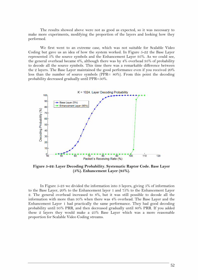
52

The results showed above were not as good as expected, so it was necessary to

make more experiments, modifying the proportion of the layers and looking how they performed.

We first went to an extreme case, which was not suitable for Scalable Video

Coding but gave us an idea of how the system worked. In Figure 5-22 the Base Layer represented 5% the source symbols and the Enhancement Layer 95%. As we could see, the general overhead became 6%, although there was by 4% overhead 95% of probability to decode all the source symbols. This time there was a remarkable difference between the 2 layers. The Base Layer maintained the good performance even if you received 20% less than the number of source symbols (PPR= 80%). From this point the decoding probability decreased gradually until PPR=50%.

Figure 5-22: Layer Decoding Probability. Systematic Raptor Code. Base Layer (5%). Enhancement Layer (95%).

In Figure 5-23 we divided the information into 3 layers, giving 5% of information

to the Base Layer, 20% to the Enhancement layer 1 and 75% to the Enhancement Layer 2. The general overhead increased to 8%, but it was still possible to decode all the information with more than 95% when there was 4% overhead. The Base Layer and the Enhancement Layer 1 had practically the same performance. They had good decoding probability until 95% PRR, and then decreased gradually until 80% PRR. If you added these 2 layers they would make a 25% Base Layer which was a more reasonable proportion for Scalable Video Coding streams.

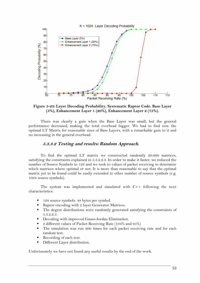
53

Figure 5-23: Layer Decoding Probability. Systematic Raptor Code. Base Layer (5%), Enhancement Layer 1 (20%), Enhancement Layer 2 (75%).

There was clearly a gain when the Base Layer was small, but the general performance decreased, making the total overhead bigger. We had to find now the optimal LT Matrix for reasonable sizes of Base Layers, with a remarkable gain to it and no increasing in the general overhead.

5.3.3.2 Testing and results: Random Approach.

To find the optimal LT matrix we constructed randomly 20.000 matrices,

satisfying the constraints explained in 5.3.2.2.3. In order to make it faster, we reduced the number of Source Symbols to 128 and we took to values of packet receiving to determine which matrices where optimal or not. It is more than reasonable to say that the optimal matrix yet to be found could be easily extended to other number of source symbols (e.g. 1024 source symbols).

The system was implemented and simulated with C++ following the next

characteristics:

128 source symbols. 48 bytes per symbol. Raptor encoding with 2 layer Generator Matrices.

The degree distributions were randomly generated satisfying the constraints of 5.3.2.2.3.

Decoding with improved Gauss-Jordan Elimination.

2 different values of Packet Receiving Rate (104% and 95%)

The simulation was run 200 times for each packet receiving rate and for each random test.

Recording of each test.

Different Layer distribution. Unfortunately we have not found any useful results by the end of the work.

54

6 Conclusions and future work

In this work we have introduced the main concepts behind the Progressive FEC for video based on the latest rateless codes. We started describing the current state of video coding. As it was showed there are many inter-dependencies in advanced video coding (e.g. H.264/AVC, SCV…) and they make part of the video data more important than other parts. On the other hand the video packets are equally erased over the transmission channel and equally recovered by the latest FEC techniques (LDPC, rateless codes...). It is obvious the need of an unequal error protection FEC code for video.

We have also checked that there is not yet a research thread on this topic and that there are only a few research papers which we have briefly described. Then we made a description of the current Raptor Code Standard [24], on which our work is based, and we described our Progressive FEC approach. Finally, we showed some results and proved that it is possible to give more protection to more important data and make them progressively recoverable before the rest of the data.

The first approach of Progressive FEC didn‟t give a remarkable gain to the Base

Layer when this represented 40% of the total information, which is a likely size from a Base Layer of a Scalable Video Coding stream. Although it gave a small increase on the total overhead, the decoding performance of the Base Layer was significantly improved when they had a small size, especially for 5%. This size is not suitable when it comes to video coding but it may be useful for other applications that use headers (e.g. Internet Protocol., wireless communication, graphics file formats, etc…). In these cases the header contains important information from the data contained in the body. It is desirable to be more protected than the rest.

The next step would be to find empirically the optimal degree distribution which

gives remarkable protection to the most important data of a video stream without increasing the good performance of the rateless codes. It could then be transformed into an automatic encoding algorithm and could be extended to any number of source symbols.

The decoding algorithm used in this approach was Gauss-Jordan elimination.

Although it is not efficient enough to be implemented in a real system it was of the outmost importance to show the potential of the Progressive FEC for video. Obviously it would be necessary an optimization of the algorithm or to find other efficient algorithms which suits our approach.

Furthermore, it would necessary to find the theoretical upper and lower bounds of

the Progressive FEC for video approach and analyze the performance asymptotically. We conclude emphasizing the difficulty of finding an appropriate degree

distribution which is the most important component responsible for the efficiency of rateless codes, and it is the key on distributing decoding probabilities. However, it is a very interesting topic and we have just opened a path on what could be the future of Progressive FEC for video.

55

7 Conclusiones y trabajo futuro

En este PFC se han introducido los conceptos principales detrás del “FEC Progresivo para video” basado en los códigos “rateless” más recientes. Comenzamos describiendo el estado actual de la codificación de vídeo. Como se vio, existen dependencias entre los datos de una fuente de video (por ejemplo, H.264/AVC, SCV...) y esto hace que parte de los datos de vídeo sean más importante otras. Existe una jerarquía. Además todos los paquetes vídeo pueden ser, con igual probabilidad, eliminados a través del canal de transmisión y también se recuperan con igual probabilidad a través de las técnicas FEC (LDPC, códigos rateless...). Se hace evidente la necesidad de un código FEC que ofrezca protección para datos de vídeo.

También comprobamos como aun no existe una vía de investigación sobre este

tema y que sólo existen unos pocos artículos científicos, que hemos descrito brevemente. Luego hicimos una descripción del actual estándar de “Raptor Code” [24], sobre el que se basa el trabajo, y describimos a continuación la aproximación “FEC Progresivo para video”. Por último, mostramos los resultados de la aproximación y demostramos que es posible dar mayor protección a los datos más importantes y que además se puede recuperar progresivamente antes que el resto.

El primer enfoque del “FEC Progresivo para video” no dio una ganancia notable

de la capa de base (datos prioritarios) cuando esta representaba el 40% de la información total, proporción razonable de datos de codificación de video escalable. Aunque hubo un pequeño incremento en el “overhead” total, la probabilidad de decodificación de la capa base fue significativamente mejor cuando tenían un tamaño pequeño, especialmente 5% de todos los datos. Este tamaño no se ajusta a la codificación de vídeo, pero puede ser útil para otras aplicaciones que utilice cabeceras (por ejemplo, Internet Protocol (IP), comunicaciones inalámbricas, formatos de archivos gráficos, etc...). En estos casos, el encabezado contiene información importante de los datos contenidos en el cuerpo y es conveniente que esté más protegido.

El siguiente paso a dar en este trabajo sería encontrar empíricamente la

distribución de grado óptima, que ofrezca una protección notable a los datos más importantes de paquetes de video, sin incrementar el buen rendimiento de los códigos “rateless”. Una vez encontrada la distribución se podría hallar un algoritmo de codificación automático para cualquier número de símbolos fuente.

El algoritmo de decodificación utilizado fue la eliminación de Gauss-Jordan.

Aunque no es lo suficientemente eficaz para ser aplicado en un sistema real era nos ha sido de máxima importancia para mostrar el potencial del “FEC Progresivo para video”. Obviamente, sería necesaria una optimización del algoritmo o encontrar otros algoritmos eficientes que conserven parecidas características.

Además, sería necesario encontrar los límites teóricos e esta aproximación y

analizar el comportamiento asintótico del código.

Concluimos haciendo hincapié en la dificultad de encontrar una distribución de

grado adecuada y de adaptar los actuales códigos “rateless”. Sin embargo, se perfila como un tema muy interesante, del cual acabamos de abrir sólo una pequeña puerta.

56

References [1] Heiko Schwarz, Detlev Marpe and Thomas Wiegand. Overview of the Scalable

Video Coding. Extension of the H.264/AVC Standard. IEEE Transactions on circuits and systems for video technology, Vol 17, No. 9, September 2007.

[2] Ahsun H. RIurad and Thomas E. Fuja. Joint-Source-Channel-Decoding of Variable

length encoded sources. Department of Electrical Engineering and Institute for Systems Research University of Maryland, College Park, 22-26 June 1998.

[3] David J.C. MacKay: Information Theory, Inference, and Learning Algorithms, ©.

Chapter 50: Digital Fountain Codes. Cambridge University Press, Version 7.2 (fourth printing) March 28, 2005.

[4] Susanna Spinsante, Ennio Gambi, Lorenzo Ciccarelli, Andrea Lorenzo Vitali, Jorge Sastre Martínez, and Paul Salama, Advances in Video Coding for Broadcast Applications, International Journal of Digital Multimedia Broadcasting, vol. 2009, Article ID 368326, 2 pages, 2009. doi:10.1155/2009/368326.

[5] Advanced Video Coding for Generic Audiovisual Services, ITU-T Rec. H.264 and

ISO/IEC 14496-10 (MPEG-4 AVC), ITU-T and ISO/IECJTC 1, Version 1: May 2003, Version 2: May 2004, Version 3: Mar.2005, Version 4: Sept. 2005, Version 5 and Version 6: June 2006, Version7: Apr. 2007, Version 8 (including SVC extension): Consented in July 2007.

[6] T. Wiegand, G. J. Sullivan, G. Bjøntegaard, and A. Luthra, Overview of the

H.264/AVC video coding standard, IEEE Trans. Circuits Syst. Video Technol., vol. 13, no. 7, pp. 560–576, Jul. 2003.

[7] Todd K. Moon (2005) Error Correction Coding, Mathematical Methods and Algorithms. Chapter 1: Introduction and Foundations. Wiley, ISBN 0-471-64800-0

[8] Frank R. Kschischang, Brendan J. Frey, and Hans-Andrea Loeliger, Factor Graphs and Sum-Product Algorithm, IEEE Transactions on Information Theory, Vol.47, pp.498-519, Feb 2001.

[9] MG Luby, M Mitzenmacher, M.A Shokrollahi, D.A Spielman. Efficient Erasure Correcting Codes. Information Theory, IEEE Transactions on, Vol. 47, No. 2. (2001), pp. 569-584.

[10] David J.C. MacKay: Information Theory, Inference, and Learning Algorithms, ©. Chapter 26: Exact Marginalization in Graphs. Cambridge University Press, Version 7.2 (fourth printing) March 28, 2005.

[11] Chapter 12: The sum-product algorithm. Principles of Digital Communication II, Spring 2005 - MIT OCW.

57

[12] David J.C. MacKay: Information Theory, Inference, and Learning Algorithms, ©. Chapter 1: Introduction to Information Theory. Cambridge University Press, Version 7.2 (fourth printing) March 28, 2005.

[13] Richard W. Hamming: Error Detection and Error Correction Codes. The Bell System

Technical Journal, Vol. XXVI 2, 1950

[14] R. G. Gallager, Low-density parity-check codes, IRE Trans. Inform. Theory, vol. IT-8, pp. 21–28, Jan. 1962.

[15] D.J.C. MacKay and R.M. Neal, Near Shannon limit performance of low density parity

check codes, IEE Electronics Letters, vol. 32, no. 18, pp. 1645-1655, 29th Aug. 1996.

[16] Tanner, R. A recursive approach to low complexity codes. Information Theory, IEEE

Transactions Sep 1981.Volume: 27, Issue: 5.pages: 533- 547.ISSN: 0018-9448

[17] J. Byers, M. Luby, M. Mitzenmacher, and A. Rege, A digital fountain approach to

reliable distribution of bulk data, in proceedings of ACM SIGCOMM ‟98, 1998.

[18] M. Luby , LT-codes, in Proc. 43rd Annu. IEEE Symp. Foundations of Computer

Science (FOCS), Vancouver, BC, Canada, Nov. 2002, pp. 271–280.

[19] Amin Shokrollahi, Raptor Codes, IEEE Transactions on Information Theory, vol.

52, pp. 2551-2567, 2006

[20] Sheng-Kai Chang, Kai-Chao Yang, and Jia-Shung Wang. Unequal-Protected LT

Code for layered video streaming. Proceedings of IEEE International Conference on

Communications, ICC 2008, Beijing, China, 19-23 May 2008.

[21] Simon S. Woo and Michael K. Cheng, Prioritized LT Codes. Information Sciences and Systems, 42nd Annual Conference. March 2008.

[22] Nazanin Rahnavard, Badri N. Vellambi, Faramarz Fekri. Rateless Codes with

Unequal Error Protection Property. Page 1. IEEE Transaction on information theory, VOL. 53, NO. 4, April 2007.

[23] M. Luby,Mitzenmacher, and A. Shokrallahi, Analysis of random processes via and-or

tree evaluation, in Proc. 9th Ann. ACM-SIAM Symp. Discrete Algorithms, 1998, pp. 364–373.

[24] M. Luby, A. Shokrollahi, M. Watson, and T. Stockhammer. (2007, September) Raptor Forward Error Correction Scheme for Object Delivery. Internet Engineering Task Force, RFC 5053. [Online]. Available: http://tools.ietf.org/html/rfc5053

[25] E. Hyytiä, T. Tirronen and J. Virtamo, Optimizing the Degree Distribution of LT Codes with an Importance Sampling Approach, in RESIM 2006, 6th International Workshop on Rare Event Simulation, Bamberg, Germany, 2006.

[26] A. Shokrollahi, S. Lassen, and R. Karp, Systems and processes for decoding chain reaction codes through inactivation, U.S.Patent 6,856,263, 2005, issued Feb 15, 2005; filed June 10, 2003.

I

Glossary Streaming Media It is multimedia that is constantly received by, and normally presented to, an end-user while it is being delivered by a streaming provider. Broadcasting In computer networking, it refers to transmitting a packet that will be received (conceptually) by every device on the network. In practice, the scope of the broadcast is limited to a broadcast domain. Contrast unicasting and multicasting. SVC - Scalable Video Coding It is the name given to an extension of the H.264/MPEG-4 AVC video compression standard. FEC - Forward Error Correction It is a system of error control for data transmission, whereby the sender adds redundant data to its messages, also known as an error correction code. This allows the receiver to detect and correct errors (within some bound) without the need to ask the sender for additional data. L-FEC – Layer-Aware Forward Error Correction. TCP- Transmission Control Protocol Transport layer protocol (L4) that is one of the core protocols of the Internet protocol suite. H.264/AVC It is a standard for video compression, and is equivalent to MPEG-4 Part 10, or MPEG-4 AVC (for Advanced Video Coding). BEC - Binary Erasure Channel This model, a transmitter sends a bit (a zero or a one), and the receiver either receives the bit or it receives a message that the bit was not received ("erased"). It counts lost information bits as being “erased” with probabilities equal to 0.5. Currently, the BEC is widely used to model the Internet transmission systems, in particular multicasting and broadcasting. DVD - Digital Video Disc DVB - Digital Video Broadcasting

II

DSL – Digital Subscriber Line UMTS – Universal Mobile Telecommunication System VGA- Video Graphics Array It is a graphics standard for personal computers and associated connectors. RGB color model - Red Green Blue color model It is an additive color model in which red, green, and blue light are added together in various ways to reproduce a broad array of colors. The name of the model comes from the initials of the three additive primary colors, red, green, and blue. VCL – Video Coding Layer NAL – Network Abstraction Layer GOP – Group of Pictures CGS - coarse-grain quality scalable coding ML – Maximum Likelihood It refers to the Maximum Likelihood Decoding Method. It is normally used to decode linear block codes. ARQ - Automatic Repeat-reQuest It is an error control method for data transmission which uses acknowledgments and timeouts to achieve reliable data transmission over an unreliable service. JSCC - Joint-Source-Channel-Coding Coding technique where source coding (compression) and channel coding (error protection) can are not performed separately and sequentially, but there are jointly optimized. LT Codes- Luby Transform Codes BP - Belief Propagation APP – A Posteriori Probability BCJR Algorithm - Bahl, Cocke, Jelinek and Raviv Algorithm It is an algorithm for maximum a posteriori decoding of error correcting codes defined on trellises.

III

MLSD - Maximum-Likelihood Sequence Detection Viterbi algorithm It is a dynamic programming algorithm for finding the most likely sequence of hidden states – called the Viterbi path – that results in a sequence of observed events. Asymptotic Performance

An algorithm has an asymptotic performance when the increase in running time as the number of nodes/variables approaches to infinity UEP – Unequal Error Protection URT – Unequal Recovery Time EEP – Equal Error Protection ESI - Encoding Symbol ID

Encoding Symbol ID values from 0 to N-1 identify the source symbols of a source block in sequential order GF(n) - Galois field with n elements. It is a field that contains only finitely many elements; all operations performed in the finite field result in an element within that field. PDF - Probability Density Function The PDF of a continuous random variable is a function which can be integrated to obtain the probability that the random variable takes a value in a given interval. Augmented matrix An augmented matrix is a matrix representation of a system of linear equations where each row of the matrix is the coefficients of the given equation and the equation's result.

I

PRESUPUESTO 1) Ejecución Material

Compra de ordenador personal (Software incluido)....... .................................. 2.000 €

Alquiler de impresora láser durante 11 meses ....................................................... 100 €

Material de oficina ........................................................................................................ 150 €

Total de ejecución material .................................................................................... 2.250 €

2) Gastos generales

16 % sobre Ejecución Material .......................................................................... 360 €

3) Beneficio Industrial

6 % sobre Ejecución Material ............................................................................ 135 €

4) Honorarios Proyecto

880 horas a 12 € / hora .................................................................................. 10560 €

5) Material fungible

Gastos de impresión ............................................................................................... 60 €

Encuadernación ..................................................................................................... 200 €

6) Subtotal del presupuesto

Subtotal Presupuesto ...................................................................................... 13070 €

7) I.V.A. aplicable

16% Subtotal Presupuesto ........................................................................... 2091.2 €

8) Total presupuesto

Total Presupuesto ........................................................................................ 15161,2 €

Madrid, Septiembre de 2009

El Ingeniero Jefe de Proyecto

Fdo.: Imanol Gómez Rubio Ingeniero Superior de Telecomunicación

3

PLIEGO DE CONDICIONES

Este documento contiene las condiciones legales que guiarán la realización, en este proyecto, de Optimización de códigos rateless aplicados a la codificación de video escalable. En lo que sigue, se supondrá que el proyecto ha sido encargado por una empresa cliente a una empresa consultora con la finalidad de realizar dicho sistema. Dicha empresa ha debido desarrollar una línea de investigación con objeto de elaborar el proyecto. Esta línea de investigación, junto con el posterior desarrollo de los programas está amparada por las condiciones particulares del siguiente pliego.

Supuesto que la utilización industrial de los métodos recogidos en el presente proyecto ha sido decidida por parte de la empresa cliente o de otras, la obra a realizar se regulará por las siguientes:

Condiciones generales

1. La modalidad de contratación será el concurso. La adjudicación se hará, por tanto, a la proposición más favorable sin atender exclusivamente al valor económico, dependiendo de las mayores garantías ofrecidas. La empresa que somete el proyecto a concurso se reserva el derecho a declararlo desierto. 2. El montaje y mecanización completa de los equipos que intervengan será realizado totalmente por la empresa licitadora. 3. En la oferta, se hará constar el precio total por el que se compromete a realizar la obra y el tanto por ciento de baja que supone este precio en relación con un importe límite si este se hubiera fijado. 4. La obra se realizará bajo la dirección técnica de un Ingeniero Superior de Telecomunicación, auxiliado por el número de Ingenieros Técnicos y Programadores que se estime preciso para el desarrollo de la misma. 5. Aparte del Ingeniero Director, el contratista tendrá derecho a contratar al resto del personal, pudiendo ceder esta prerrogativa a favor del Ingeniero Director, quien no estará obligado a aceptarla. 6. El contratista tiene derecho a sacar copias a su costa de los planos, pliego de condiciones y presupuestos. El Ingeniero autor del proyecto autorizará con su firma las copias solicitadas por el contratista después de confrontarlas. 7. Se abonará al contratista la obra que realmente ejecute con sujeción al proyecto que sirvió de base para la contratación, a las modificaciones autorizadas por la superioridad o a las órdenes que con arreglo a sus facultades le hayan comunicado por escrito al Ingeniero Director de obras siempre que dicha obra se haya ajustado a los preceptos de los pliegos de condiciones, con arreglo a los cuales, se harán las modificaciones y la valoración de las diversas unidades sin que el importe total pueda exceder de los presupuestos aprobados. Por consiguiente, el número de unidades que se consignan en el proyecto o en el presupuesto, no podrá servirle de fundamento para entablar reclamaciones de ninguna clase, salvo en los casos de rescisión. 8. Tanto en las certificaciones de obras como en la liquidación final, se abonarán los trabajos realizados por el contratista a los precios de ejecución material que figuran en el presupuesto para cada unidad de la obra.

4

9. Si excepcionalmente se hubiera ejecutado algún trabajo que no se ajustase a las condiciones de la contrata pero que sin embargo es admisible a juicio del Ingeniero Director de obras, se dará conocimiento a la Dirección, proponiendo a la vez la rebaja de precios que el Ingeniero estime justa y si la Dirección resolviera aceptar la obra, quedará el contratista obligado a conformarse con la rebaja acordada. 10. Cuando se juzgue necesario emplear materiales o ejecutar obras que no figuren en el presupuesto de la contrata, se evaluará su importe a los precios asignados a otras obras o materiales análogos si los hubiere y cuando no, se discutirán entre el Ingeniero Director y el contratista, sometiéndolos a la aprobación de la Dirección. Los nuevos precios convenidos por uno u otro procedimiento, se sujetarán siempre al establecido en el punto anterior. 11. Cuando el contratista, con autorización del Ingeniero Director de obras, emplee materiales de calidad más elevada o de mayores dimensiones de lo estipulado en el proyecto, o sustituya una clase de fabricación por otra que tenga asignado mayor precio o ejecute con mayores dimensiones cualquier otra parte de las obras, o en general, introduzca en ellas cualquier modificación que sea beneficiosa a juicio del Ingeniero Director de obras, no tendrá derecho sin embargo, sino a lo que le correspondería si hubiera realizado la obra con estricta sujeción a lo proyectado y contratado. 12. Las cantidades calculadas para obras accesorias, aunque figuren por partida alzada en el presupuesto final (general), no serán abonadas sino a los precios de la contrata, según las condiciones de la misma y los proyectos particulares que para ellas se formen, o en su defecto, por lo que resulte de su medición final. 13. El contratista queda obligado a abonar al Ingeniero autor del proyecto y director de obras así como a los Ingenieros Técnicos, el importe de sus respectivos honorarios facultativos por formación del proyecto, dirección técnica y administración en su caso, con arreglo a las tarifas y honorarios vigentes. 14. Concluida la ejecución de la obra, será reconocida por el Ingeniero Director que a tal efecto designe la empresa. 15. La garantía definitiva será del 4% del presupuesto y la provisional del 2%. 16. La forma de pago será por certificaciones mensuales de la obra ejecutada, de acuerdo con los precios del presupuesto, deducida la baja si la hubiera. 17. La fecha de comienzo de las obras será a partir de los 15 días naturales del replanteo oficial de las mismas y la definitiva, al año de haber ejecutado la provisional, procediéndose si no existe reclamación alguna, a la reclamación de la fianza. 18. Si el contratista al efectuar el replanteo, observase algún error en el proyecto, deberá comunicarlo en el plazo de quince días al Ingeniero Director de obras, pues transcurrido ese plazo será responsable de la exactitud del proyecto. 19. El contratista está obligado a designar una persona responsable que se entenderá con el Ingeniero Director de obras, o con el delegado que éste designe, para todo relacionado con ella. Al ser el Ingeniero Director de obras el que interpreta el proyecto, el contratista deberá consultarle cualquier duda que surja en su realización. 20. Durante la realización de la obra, se girarán visitas de inspección por personal facultativo de la empresa cliente, para hacer las comprobaciones que se crean oportunas. Es obligación del contratista, la conservación de la obra ya ejecutada hasta la recepción de la misma, por lo que el deterioro parcial o total de ella, aunque sea por agentes atmosféricos u otras causas, deberá ser reparado o reconstruido por su cuenta.

5

21. El contratista, deberá realizar la obra en el plazo mencionado a partir de la fecha del contrato, incurriendo en multa, por retraso de la ejecución siempre que éste no sea debido a causas de fuerza mayor. A la terminación de la obra, se hará una recepción provisional previo reconocimiento y examen por la dirección técnica, el depositario de efectos, el interventor y el jefe de servicio o un representante, estampando su conformidad el contratista. 22. Hecha la recepción provisional, se certificará al contratista el resto de la obra, reservándose la administración el importe de los gastos de conservación de la misma hasta su recepción definitiva y la fianza durante el tiempo señalado como plazo de garantía. La recepción definitiva se hará en las mismas condiciones que la provisional, extendiéndose el acta correspondiente. El Director Técnico propondrá a la Junta Económica la devolución de la fianza al contratista de acuerdo con las condiciones económicas legales establecidas. 23. Las tarifas para la determinación de honorarios, reguladas por orden de la Presidencia del Gobierno el 19 de Octubre de 1961, se aplicarán sobre el denominado en la actualidad “Presupuesto de Ejecución de Contrata” y anteriormente llamado ”Presupuesto de Ejecución Material” que hoy designa otro concepto.

Condiciones particulares

La empresa consultora, que ha desarrollado el presente proyecto, lo entregará a la empresa cliente bajo las condiciones generales ya formuladas, debiendo añadirse las siguientes

condiciones particulares: 1. La propiedad intelectual de los procesos descritos y analizados en el presente trabajo, pertenece por entero a la empresa consultora representada por el Ingeniero Director del Proyecto. 2. La empresa consultora se reserva el derecho a la utilización total o parcial de los resultados de la investigación realizada para desarrollar el siguiente proyecto, bien para su publicación o bien para su uso en trabajos o proyectos posteriores, para la misma empresa cliente o para otra. 3. Cualquier tipo de reproducción aparte de las reseñadas en las condiciones generales, bien sea para uso particular de la empresa cliente, o para cualquier otra aplicación, contará con autorización expresa y por escrito del Ingeniero Director del Proyecto, que actuará en representación de la empresa consultora. 4. En la autorización se ha de hacer constar la aplicación a que se destinan sus reproducciones así como su cantidad. 5. En todas las reproducciones se indicará su procedencia, explicitando el nombre del proyecto, nombre del Ingeniero Director y de la empresa consultora. 6. Si el proyecto pasa la etapa de desarrollo, cualquier modificación que se realice sobre él, deberá ser notificada al Ingeniero Director del Proyecto y a criterio de éste, la empresa consultora decidirá aceptar o no la modificación propuesta. 7. Si la modificación se acepta, la empresa consultora se hará responsable al mismo nivel que el proyecto inicial del que resulta el añadirla. 8. Si la modificación no es aceptada, por el contrario, la empresa consultora declinará toda responsabilidad que se derive de la aplicación o influencia de la misma.

6

9. Si la empresa cliente decide desarrollar industrialmente uno o varios productos en los que resulte parcial o totalmente aplicable el estudio de este proyecto, deberá comunicarlo a la empresa consultora. 10. La empresa consultora no se responsabiliza de los efectos laterales que se puedan producir en el momento en que se utilice la herramienta objeto del presente proyecto para la realización de otras aplicaciones. 11. La empresa consultora tendrá prioridad respecto a otras en la elaboración de los proyectos auxiliares que fuese necesario desarrollar para dicha aplicación industrial, siempre que no haga explícita renuncia a este hecho. En este caso, deberá autorizar expresamente los proyectos presentados por otros. 12. El Ingeniero Director del presente proyecto, será el responsable de la dirección de la aplicación industrial siempre que la empresa consultora lo estime oportuno. En caso contrario, la persona designada deberá contar con la autorización del mismo, quien delegará en él las responsabilidades que ostente.