PROPERTIES OF RANDOM MATRICES AND APPLICATIONScvs/coding/random_report.pdf · PROPERTIES OF RANDOM...
37
PROPERTIES OF RANDOM MATRICES AND APPLICATIONS IAN F. BLAKE AND CHRIS STUDHOLME Abstract. This report surveys certain results on random matrices over finite fields and their applications, especially to coding theory. Extensive experimental work on such ma- trices is reported on and resulting conjectures are noted. December 15, 2006 1. Introduction The study of random matrices over a finite field arises most naturally in a variety of contexts covered by the term ”probabilistic combinatorics”. Perhaps the prime example of this area is the study of graphical evolution, and in particular the study of threshold phenomena on graphs as more edges are added in a prescribed random manner to a set of graph vertices. However, many other aspects, such as the study of random permutations, random equations over finite fields, and many others are also of importance. The particular application of interest in this report is to the study of rank properties of rectangular matrices over finite fields, and their use in coding theory. The intent is a compilation and survey of relevant results of interest. It is by no means encyclopdaeic. The only contribution of the report is in the experimental results given in section 6. Our main interest will be the study of rank properties of random k × (k + m) matrices where m> −k, over F q which will be designated M k,k+m (q). The q will be omitted if it is understood. When interest is restricted to square matrices over F q of size n × n we will use the notation M n (q), to emphasize the difference, and again omit the q when it is understood. In either the square or rectangular case, we say the matrix is of full rank if it has rank min(k,k + m) (or n, respectively). Where possible, we adapt results from the literature to this notation and note where this has not been done. Later, the notation will be modified to accommodate the probability with which each element of the finite field is chosen. The reader is reminded of the standard algorithmic complexity notation [13] for a function of an integer N, f (N ): i) g(N )= O(f (N )) iff | g(N )/f (N ) | is bounded from above as N →∞ ii) g(N )= o(F (N )) iff g(N )/f (N ) → 0 as N →∞ iii) g(N ) = Ω(N ) iff | g(N )/f (N ) | is bounded from above by a strictly positive number as iv) g(N ) = Θ(N ) iff | g(N )/f (N ) | is bounded both from above and below by a strictly positive number as N →∞. Date : March, 2006. 1991 Mathematics Subject Classification. Primary 54C40, 14E20; Secondary 46E25, 20C20. Key words and phrases. random matrices, bipartite graphs, coding theory. The first author was supported in part by NSERC Grant A632. 1
Transcript of PROPERTIES OF RANDOM MATRICES AND APPLICATIONScvs/coding/random_report.pdf · PROPERTIES OF RANDOM...
PROPERTIES OF RANDOM MATRICES AND APPLICATIONS
IAN F. BLAKE AND CHRIS STUDHOLME
Abstract. This report surveys certain results on random matrices over finite fields and
their applications, especially to coding theory. Extensive experimental work on such ma-
trices is reported on and resulting conjectures are noted.
December 15, 2006
1. Introduction
The study of random matrices over a finite field arises most naturally in a variety of
contexts covered by the term ”probabilistic combinatorics”. Perhaps the prime example
of this area is the study of graphical evolution, and in particular the study of threshold
phenomena on graphs as more edges are added in a prescribed random manner to a set of
graph vertices. However, many other aspects, such as the study of random permutations,
random equations over finite fields, and many others are also of importance. The particular
application of interest in this report is to the study of rank properties of rectangular matrices
over finite fields, and their use in coding theory. The intent is a compilation and survey of
relevant results of interest. It is by no means encyclopdaeic. The only contribution of the
report is in the experimental results given in section 6.
Our main interest will be the study of rank properties of random k × (k + m) matrices
where m > −k, over Fq which will be designated Mk,k+m(q). The q will be omitted if
it is understood. When interest is restricted to square matrices over Fq of size n × n we
will use the notation Mn(q), to emphasize the difference, and again omit the q when it is
understood. In either the square or rectangular case, we say the matrix is of full rank if
it has rank min(k, k + m) (or n, respectively). Where possible, we adapt results from the
literature to this notation and note where this has not been done. Later, the notation will
be modified to accommodate the probability with which each element of the finite field is
chosen.
The reader is reminded of the standard algorithmic complexity notation [13] for a function
of an integer N, f(N): i) g(N) = O(f(N)) iff | g(N)/f(N) | is bounded from above
as N → ∞ ii) g(N) = o(F (N)) iff g(N)/f(N) → 0 as N → ∞ iii) g(N) = Ω(N) iff
| g(N)/f(N) | is bounded from above by a strictly positive number as iv) g(N) = Θ(N)
iff | g(N)/f(N) | is bounded both from above and below by a strictly positive number as
N → ∞.
Date: March, 2006.
1991 Mathematics Subject Classification. Primary 54C40, 14E20; Secondary 46E25, 20C20.
Key words and phrases. random matrices, bipartite graphs, coding theory.
The first author was supported in part by NSERC Grant A632.
1

2 IAN F. BLAKE AND CHRIS STUDHOLME
The outline of the report is as follows: The next section gives the well known enumer-
ation of certain subspaces of vectors spaces over finite fields. The following two sections
discuss random matrices, especially their rank properties, over F2 and Fq, q > 2. Section 5
considers other aspects of of both random and nonrandom matrices that are relevant to our
interests. These include the properties of windowed random matrices, and the algorithmic
construction of rectangular matrices with the property that each column has a maximum
weight and any k columns are independent. Some questions relating to the eigenvalues of
random matrices and certain randomness questions of some matrix groups are noted.
Section 6 reports extensively on experiments with certain rank properties of random
matrices. This leads to certain conjectures believed to be of interest. This is followed by
a section on codes for the erasure channel that are derived from the windowed matrices
previously considered. These codes, while having a slightly increased decoding complexity,
have a very low overhead and high probability of decoding completion.
It is empasized again that, apart from the experimental data generated, the report is
a compilation of certain of the approaches to these matrices found in the literature. It is
intended only as a summary of certain of the approaches of interest.
2. A preliminary result
Let Vn(q) denote the vector space of dimension n over the finite field Fq The number of
ways of choosing a basis for Vn(q) is easily determined as
(qn − 1)(qn − q) · · · (qn − qn−1) = qn(n−1)/2n
∏
i=1
(qi − 1).
Likewise the number of ways of choosing a basis of a k dimensional subspace of Vn(q) is
(qn − 1)(qn − q) · · · (qn − qk−1)
and for each such subspace there are
(qk − 1)(qk − q) · · · (qk − qk−1)
ways of choosing a basis. Thus the number of distinct k-dimensional subspaces of Vn(q), a
quantity we denote by[n
k
]
q, is
[n
k
]
q=
k−1∏
i=0
(qn−i − 1)
(qk−i − 1).
The quantities[n
k
]
qare referred to as Gaussian coefficients and enjoy many properties that
are similar to those of ordinary binomial coefficients (e.g. [4]):
[n
k
]
q=
[n − 1
k − 1
]
q+
[n − 1
k
]
qand
[n
k
]
q=
(qn − 1)
(qk − 1)
[n − 1
k − 1
]
q.
It is easy to see that one can view[
nk
]
qas a polynomial (not a rational function) in q and,
if one replaces q with 1 in this polynomial, one obtains(nk
)
([29]).
One has the following theorem ([29]):
PROPERTIES OF RANDOM MATRICES AND APPLICATIONS 3
Theorem 2.1 ([29], page 303). The number of surjective linear transformations from an
n-dimensional vector space Vn(q) to an m-dimensional vector space over Fq is
(2.1)
m∑
k=0
(−1)m−k[m
k
]
qqnk+(m−k
2 ).
The proof (omitted here) uses Mobius inversion on the lattice of subspaces of the vector
space Vn(q). An important corollary of this theorem for our purposes is ([29]), recast with
the notation we will use in the sequel, is:
Corollary 2.2. The number of k × n matrices over Fq that have rank r is
(2.2) Nq(k, n, r) =[n
r
]
q
r∑
ℓ=0
(−1)r−ℓ[r
ℓ
]
qqkℓ+(r−ℓ
2 ).
Here, the first Gaussian coefficient is the number of distinct subspaces of an n-dimensional
space of dimension r and the summation is the number of surjective maps from a k-
dimensional space to an r-dimensional one and the result follows.
Our interest in subsequent sections will be in k×(k+m) matrices wth m > −k, (m+k >
0).
3. Random matrices over F2
The problem of determining the probability that a set of m randomly chosen k-tuples
over a finite field F2 are linearly independent (over a F2) is quite old. As noted earlier, we
denote by Mk,k+m(q) a k×(k+m) random matrix, over the finite field Fq. We will normally
be interested in the case where m ≥ 0 but will also consider the case for −k ≤ m ≤ 0. When
the finite field is understood we delete the q in the matrix notaton. Denote by ρ(Mk,k+m) the
rank of the matrix (≤ min(k, k+m)). If this probability is denoted Qk,k+m then Berlekamp
[2] (adapted to our notation) gives the argument (credited to Lansdurg [17]) that for m ≤ 0
P (ρ(Mk,k+m) = k + m) =
k+m−1∏
j=0
(
1 − 1
2k−j
)
, −k ≤ m ≤ 0.
For k → ∞ for fixed m ≥ 0, then we will see that
Pρ(Mk,k+m) = k) = Qm =
∞∏
i=−m+1
(
1 − 1
2i
)
,m ≥ 0.
A useful rapidly converging form ([2]) of this equation is
log Qm =∞∑
i=m+1
log(1 − 2−i) =∞∑
j=1
−2−sj
j(2j − 1), s ≥ 0.
In particular it is noted that
Q0 =∞∏
j=1
(1 − 1
2j) = 0.2887880951 · · ·

4 IAN F. BLAKE AND CHRIS STUDHOLME
i.e. the probability a square random binary matrix is nonsingular as its dimension tends to
infinity. As will be noted later, this expression is very accurate even for k as low as 10.
For future reference we give an interesting approximation of Brent et al [7]. Denote by
(3.1) η(n, x) = (1 − x)(1 − x2) · · · (1 − xn)
and from the above it is clear we will have interest in expressions of the form η(n, 1/q). A
very simple and useful argument gives the result (m ≥ 0)
k∏
i=1
(
1 − 1
qm+i
)
=
0.288 q = 2 m = n,
1 − 1qm(q−1) otherwise .
To see this, note that for m ≥ n we have
η(m,x)η(m−n,x) = (1 − xm−n+1)(1 − xm−n+2) · · · (1 − xm)
≥ 1 − (xm−n+q + xm−n+2 + · · · + xm)
≥ 1 − xm−n+1(1 + x + x2 + · · · + xn−1 + · · · )≥ 1 − xm−n+1 · 1
1−x
from which the second result follows. When q = 2 and m = n the bound is zero and for
this case we compute:(
1 − 12
)(
1 − 122
)
· · ·(
1 − 12m
)
>∏∞
i=1
(
1 − 12i
)
>(
1 − 12
)(
1 − 122
)(
1 − 123
)(
1 − 124
)
(1 −(
125 + · · · + 1
2m + · · ·)
)
=(
1 − 12
)(
1 − 122
)(
1 − 123
)(
1 − 124
)
(1 −(
124
)
> 0.288.
The problems of random matrices over finite fields (especially binary) and their applica-
tions to graph theory, owe much to researchers in the former Soviet union. We begin by
considering the work of Kolchin ([16]) and transfer his results to the notation of interest
here. Namely, we are interested in the probabilty a k × (k + m) binary (i.e. over F2, al-
though there are many results for arbitrary finite fields Fq) matrix having rank r = k − s
for s ≥ 0, m + s ≥ 0. Clearly, if the matrix entries are chosen independently and equally
likely (P (aij = 0) = 1/2), the number of such matrices is N(k, k + m, r)2 as in equation
(2.1) and the matrices are equally likely and the result is
N(k, k + m, r)2/2k(k+m).
Kolchin gives a different argument as follows:
Theorem 3.1 ([16], page 126, adapted). Let Mk,k+m be a binary random k× (k+m), m >
−k, matrix with entries chosen equally likely and ρ(Mk,k+m) its rank (over F2). It will
be convenient to denote the rank by ρ(Mk,k+m) = r = k − s, s ≥ 0 Then for k − s ≤min(k, k + m), as k → ∞ we refer to s as the nullity or defect of the matrix and we have:
P (ρ(Mk,k+m) = k − s) → 2−(s)(m+s)∞∏
i=s+1
(
1 − 1
2i
)
m+s∏
i=1
(
1 − 1
2i
)−1,
where the last product is 1 if m + s = 0 (i.e. the matrix is of full rank).
PROPERTIES OF RANDOM MATRICES AND APPLICATIONS 5
Proof : (informal) The proof technique is interesting and an indication of it is given.
Consider adding random binary columns, random k-tuples over F2, to the matrix, column
by column. If the matrix is currently of size k × (k + m − 1) and rank j (the k + m − 1
columns span a j dimensional space) the probability the (k + m)-th column is in this space
is 2j/2k. Hence the probability the rank is increased by one with the added column is
1 − 2j
2k.
There is an easy case to dispose of, that of full rank when m + s = 0. In this case,
to achieve full rank, the rank must increase by one each time a column is added and the
probability of this is
P (ρ(Mk,k−s) = k − s) =
k−s−1∏
j=0
(
1 − 2j
2k
)
=
k∏
i=s+1
(
1 − 1
2i
)
, s ≥ 0.
In the general case, we consider the rank as a discrete Markov chain as a function of
the number of columns and for convenience denote ρ(Mk,k+m) by ρk+m as the rank of the
k × (k + m) matrix. Denote by ξℓ the random variable which takes on the value 1 if the
ℓ-th column increases the rank (by one) and zero otherwise. We have the probabilities:
P (ξℓ = 0 | ρℓ−1 = a) = 2a/2k, and P (ξn = 1 | ρℓ−1 = a) = 1 − 2a/2k.
The probability the rank of the k × (k + m) matrix is k − s is then the probability exactly
k − s of the (independent) random variables ξ1, ξ2, · · · , ξk+m have the value 1. Thus,
suppressing our previous notation using Mk,k+m, assuming the ranks remained the same
when columns R = 1 ≤ i1, i2, · · · , im+s ≤ k +m were added, (note that k +m− (k− s) =
m + s and that Rc is the complement set in [1, k + m]) we have:
P (ρk+m = k − s) =∑
ia∈R,jb∈Rc
∏m+sa=1 P (ξia = 0)
∏k−sb=1 P (ξjb
= 1)
=∑
1≤i1≤i2≤···≤ik+m≤n
(
1 − 12k
)(
1 − 22k
)
· · ·(
1 − 2k−s+1
2k
)
×2i1−1+i2−2+···+im+s−(m+s)
2k(m+s) .
Notice that the product term here is independent of the particular instances of when the
rank increases (ξj = 1) and so this last equation can be written as
(3.2)P (ρk+m = k − s) = 2−k(m+s)
∏k−s−1j=0
(
1 − 2j
2k
)
×∑
1≤i1≤i2≤···≤im+s≤n 2i1−1+i2−2+···+im+s−(m+s).
Notice that 1 ≤ i1 < i2 < · · · < im+s ≤ k + m and so
0 ≤ i1 − 1 ≤ i2 − 2 ≤ · · · ≤ im+s − (m + s) ≤ k − s.
If we define the variables jℓ = k − s − (iℓ − ℓ), ℓ = 1, · · · ,m + s then we have
0 ≤ jm+s ≤ · · · ≤ j1 ≤ k − s.
Considering equation 3.2, noting that k(m + s) = (k − s)(m + s) + s(m + s) to account
for the subtraction of the rank, k − s, from each index in the exponent, and reversing the
6 IAN F. BLAKE AND CHRIS STUDHOLME
product variable (replace i with k − i) we can rewrite the equation as
(3.3)P (ρk+m = k − s) = 2−s(m+s)
∏ki=s+1
(
1 − 12i
)
×∑
0≤jm+s≤jm+s−1≤···≤j1≤k−s 2−jm+s−jm+s−1+···−j1.
We examine the equation as k → ∞ and note the product term tends to∞∏
i=s+1
(
1 − 1
2i
)
.
To evaluate the sum term in 3.3 (over all possible values of the variables jℓ as k → ∞ we
have:∑
0≤jm+s≤jm+s−1≤···≤j1
2−jm+s−jm+s−1+···−j1
=∑
0≤jm+s≤jm+s−1≤···≤j22−jm+s−jm+s−1+···−j2
∑
j2≤j12−j1
=∑
0≤jm+s≤jm+s−1≤···≤j22−jm+s−jm+s−1+···−j22−j2(1 − 1
2)−1
=∑
0≤jm+s≤jm+s−1≤···≤j22−jm+s−jm+s−1+···−j3
∑
j3≤j22−2j2(1 − 1
2)−1
=∑
0≤jm+s≤jm+s−1≤···≤j22−jm+s−jm+s−1+···−j3(1 − 1
22 )−1(1 − 12)−1
and so on. The final expression is then as stated in the theorem.
Notice that the probability a random k × k binary matrix Mk is of full rank k as k
becomes large tends to the constant
P (ρ(Mk) = k) →∞∏
i=1
(
1 − 1
2i
)
= 0.2887880951 · · · .
More generally, the probability a random k× (k+m) binary matrix Mk,(k+m) is of full rank
k for m ≥ 0, for large k is
(3.4) Qm =
∞∏
i=m+1
(
1 − 1
2i) ,m = 0, 1, · · · .
If we let Pm, m ≥ 0, denote the probability that exactly m columns beyond k are needed
to obtain rank k for the k × (k + m) matrix, then
Pm = Qm − Qm−1
and the average number of extra columns needed for full rank is
m =
∞∑
m=0
mPm =
∞∑
i=0
(1 − Qi) = 1.60669515 · · · .
The simple bounds established by Brent atl [7] noted earlier can be useful for establishing
bounds when working with such expressions.
It is interesting to observe that for such a matrix only two extra columns, on average,
beyond the k, are required to achieve a full rank matrix and this, asymptotically, is inde-
pendent of k. With 7 or 8 extra columns, the probability of achieving full rank is very close
to 1 for even very small. While the above expressions are for large k, it has been observed
experimentally that the expressions are remarkably accurate for k as small as 10.
The above result depends on the fact that, as a column (a randomly chosen binary k-
tuple) is added to the matrix, the probability the rank of the matrix is increased depends

PROPERTIES OF RANDOM MATRICES AND APPLICATIONS 7
only on the current rank of the previous columns of the matrix. This assumes that the
probability the added column is in the column space of the previously chosen columns is
proportional to the size of the current columns space i.e. 2ℓ/2k if the current rank is ℓ.
Indeed, if the new column being added is not sufficiently random in being chosen, this
observation may not hold.
It seems somewhat surprising then that the previous results do not depend on the matrix
elements being chosen equally likely. In fact, as will be shown later in the work of Kolchin
and Cooper (due in some part to several other Russian mathematicians whose work is in
Russian and not used in this survey), as long as the probabilities tend to zero in a carefully
prescribed manner, the same results will hold. The following result of Kolchin is one form
of this kind of result.
Theorem 3.2 ([16], page 131, adapted). Let the elements of a random binary k × (k + m)
matrix be independently chosen and suppose there is a constant δ such that the probabilities
p(k)ij of elements aij being 1 satisfy the inequalities
δ ≤ p(k)ij ≤ 1 − δ, i = 1, 2, · · · , k, j = 1, 2, · · · k + m,
hold. Let s ≥ 0, and m be fixed integers, m + s ≥ 0. Then as k → ∞ we have
P (ρk(Mk,k+m) = k − s) → 2−s(m+s)∏∞
i=s+1
(
1 − 12i
)∏m+s
i=1
(
1 − 12i
)−1,
where the last product is 1 if m + s = 0.
The proof of the theorem is not given in [16]. However a variety of other results in the
same direction, namely on the insensitivity of the results to variations in the matrix element
probabilities, are available and some of these are noted here.
Let A be an k × (k + m) binary random matrix, then under fairly broad conditions on
the probability distribution of the matrix elements, it is shown that the mean number of
nonzero solutions to the matrix equation
XA = 0
tends to 2−m as k → ∞, where m is allowed to be negative. For m negative, the statement
is a reflection of the expected number of vectors in the null space of the matrix (and hence
of the expected rank of the null space). For m positive it simply reflects the probability the
null space is of full rank, in some sense. The proof of this result is given in [16]. Perhaps of
more interest is the fact the result remains true if the matrix element probabilities satisfy
the inequalitieslog k + x
k≤ p
(k)ij ≤ 1 − log k + x
kwhere x is a constant. This result is made sharper in the work of Cooper to be discussed
in the next section.
We pursue the ideas a little further. Let A = Ak,k+m be a random binary k × (k + m)
matrix. If columns i1, i2, · · · , ir sum to the zero k-tuple we call the set of indices C =
i1, i2, · · · , ir a critical set. Note that if C1 6= C2 are critical sets then their symmetric
difference C1∆C2 is also a critical set. One can then naturally define independent critical

8 IAN F. BLAKE AND CHRIS STUDHOLME
sets. Clearly the maximum number of independent critical sets is the dimension of the null
space of the matrix A, s(A), (and the sum of this and the rank of the matrix is k + m).
Suppose now that the elements of the matrix A are chosen independently according to
the distribution
(3.5) P [aij = 1] = p(k)ij =
log k + x
k, and P [aij = 0] = 1 − log k + x
k
where x is a constant. The limit distribution for the dimension of the null space of A, s(A)
can then be found. In particular we have
Theorem 3.3 ([16], p. 135, theorem 3.3.1). If k, k + m → ∞ such that (k + m)/k →α < 1 and the condition (3.5) is true, then the random variable s(A) (maximum number of
independent critical sets or rank of the null space) converges to a Poisson distribution with
parameter λ = αe−x.
A restatement of the theorem is, as noted in [10] (attributed to Balakin [1] and discussed
in [16] (Theorem 3.3.2, page 142, adapted), if Ak,k+m is a random matrix over F2, m ≥ 0
and p = (ln(k) + d)/k, a = (k/(k + m)) then
(3.6) P (ρ(Ak,k+m = k − s) ∼ (ae−d)k
k!e−ae−d
.
Furthermore it is shown that under the above conditions, the number of all zero columns
of the matrix A has a Poisson distribution with parameter λ = αe−d if (k + m)/k → α for
0 < α < ∞, a simple approximation of the binomial distribution. Further, if, under the
previous conditions, and (k + m)/k → α < 1 then indeed, with probability tending to 1,
the critical sets of A consist only of zero columns.
Similar to the above theorem we have:
Theorem 3.4 ([16] p. 142, theorem 3.3.2). Under the conditions 3.5, if k, (k+m) → ∞ such
that (k + m)/k → α > 1 then the distribution of s(A) converges to a Poisson distribution
with parameter λ = e−d/α.
We have been a little informal with stating the results. In [16] a more precise statement
of the results states that for a T × n matrix over F2, if n, T → ∞ in such a way that
T/n → a, constant, either a > 1 or a < 1, the results hold.
In essence it was shown that in the equiprobable case as k → ∞ the probability the matrix
Ak,k+m is of full rank tends to 1, under the conditions stated. The results are nontrivial to
prove.
Similar results can be obtained for nonhomogeneous equations AX = B and many other
aspects of the problem are treated in [16].
We note one further aspect of the conditions in equation 3.5. Suppose we let the proba-
bility of a 1 element in the matrix be
(3.7) p =log(k) + x
k
PROPERTIES OF RANDOM MATRICES AND APPLICATIONS 9
where we view x as a constant. Suppose further that (k+m)/k → α = constant, 0 < α < ∞.
Then the probability of generating an all zero column is
pk =(
1 − log(k) + x
k
)k
and as k → ∞ in such a way that (k + m)/k is constant then the probability of an all zero
column tends to pk = e−x/k. Thus, the ’threshold value’ of p = ln(k)/k noted above (and
later, in the work of Cooper [9, 10] to be discussed) is somewhat natural. Similarly, if we
take p = (c ln(k) + x)/k for c > 0, then pk → e−x/kc and as c decreases the probability
increases. A similar argument applied to rows, is more persuasive as to this threshold, since
such a matrix with an all-zero row cannot be nonsingular. The expected number of all
zero columns in the matrix then is (k + m)pk → αe−x, a constant. For lower values of p
one would thus expect the number of all zero columns to increase as k increases. Thus the
probability of a 1 in the matrix given by 3.7 leads to an expected constant number of all
zero columns which perhaps explains somewhat the threshold effect of the probability.
4. Random matrices over Fq, q > 2
The threshold probability, mentioned in the previous section, of the probability of a one
in the random binary n × n matrix being
p =log(n) − c
n
and its relationship to the number of zero rows or columns is explored further in a series
of papers ([5], [9]. [10]) by extending the work to matrices over Fq and obtaining sharper
estimates of the bound on the threshold probabilities. They consider only a square n × n
matrix Mn over Fq, q > 2, where the probability of a zero element is given by 1 − p where
p = (log(n) − c)/n for some constant c where the probability of each nonzero element is
equally likely at p/(q − 1). They observe that if one desires an expected rank of n − O(1)
then this is the critical probability, as noted previously and commented on further below. It
is also shown that the rank of such a random matrix is, with high probability, not much less
than its expected rank. In fact, the main technical result of the paper [5] is that the number
of linear dependencies of the rows (or columns) of the matrix is bounded by a constant iff
p ≥ (log(n) − c)/n where c is some fixed positive constant.
If we ask the further question as to how small p can be chosen so that a random matrix
is nonsingular (asymptotically with n) with some constant probability, then it seems the
techniques of this paper [5] are insufficient to answer this question. This question is consid-
ered in the work of Cooper ([9], [10]) to be considered later. Notice that it is already shown
that this is the case for random binary matrices (the constant .288...). (The proof in [25]
that this is not the case is erroneous). Also it would be of interest to show that p can be
nonconstant through the matrix elements, while preserving the property that the random
matrix is nonsingular (asymptotically) with some constant probability.
We informally discuss the results of the paper [5] and adopt and adapt their notation.
As before denote by Mn an n × n random matrix over Fq whose elements are chosen
independently with the probability of a zero element given by 1−p where p = (log(n)−c)/n

10 IAN F. BLAKE AND CHRIS STUDHOLME
for some constant c and the probabilities of nonzero elements equally likely at p/(q − 1).
Denote by δ(Mn) the defect or nullity, (dimension of the null space) of the matrix Mn i.e.
δ(Mn) = n − ρ(Mn), where, as before ρ(Mn) is the rank. (Note: we have used s = δ here,
but maintain the dual notation!)
We give the following sequence of theorems and corollaries of that paper with minor
adaptation of notation.
Theorem 4.1 ([5], theorem 2.1). Let Mn be a random n × n matrix over the fixed finite
field Fq (the probability of a nonzero element being p/(q − 1)) with p = (log(n) − c)/n with
n ≥ ec for a fixed c ≥ 0. Then the defect δ(Mn) satisfies
E(qδ(Mn)) = O(1).
Moreover, if the expectation is considered as a function of p then it is monotonically de-
creasing as a function in the range 0 ≤ p ≤ (q − 1)/q.
(Note: The last sentence of this theorem seems to require some clarification in that it
does not seem to rule out that, for a constant n and c, if p < (ln(n) − c)/n the size of the
null space increases as p decreases.)
The theorem implies in particular that for p above the threshold value, p = (log(n)−c)/n
for c a constant, (in fact for (ln(n) − c)/n < p < (q − 1)/q) the number of possible linear
dependencies (rows or columns) is upper bounded by a constant. Values of p close to the
threshold are of particluar interest.
The following theorem addresses the possibility of p being a function of n to see what
can be said about the rank behavior of the matrix in that case.
Theorem 4.2 ([5], theorem 2.2). Let Mn be a random matrix over Fq as before with
p(n) = (log(n) − c(n))/n for 0 ≤ c(n) < log(n) − log(q − 1). Then the defect of Mn
satisfies
E(qδ(Mn)) = Ω(e[(q−1)/4]ec
).
The expected number of all zero rows of Mn is Ω(ec).
Corollary 4.3 ([5], Corollary 2.3). Let c(n) be a function with 0 ≤ c(n) < log(n) for all n.
Then E(δ(Mn)) = O(1) for random n × n matrices over Fq with p = (log(n) − c(n))/n iff
the function c(n) is bounded.
Corollary 4.4 ([5], Corollary 2.4). For every c ≥ 0 there exists a constant Ac such that a
random n × n matrix Mn, n > ec, with p = (log(n) − c)/n satisfies
P (δ(Mn) ≥ ℓ) ≤ Ac
qℓ
for all positive integers ℓ.
Recall that a linear dependency among the rows (or columns) of the matrix Mn is a
nontrivial linear sum of rows adding to the zero row (critical set of indices in the terminology
of Kolchin). Let ℓ(Mn) be the number of such dependencies and note that ℓ(Mn) = qδ(Mn)−1. The proof of the first of these theorems depends on the following:
PROPERTIES OF RANDOM MATRICES AND APPLICATIONS 11
Theorem 4.5 ([5], theorem 3.3). Let Mn be a random n×n matrix over Fq for an arbitrary
p, 0 < p < 1. Then
E(ℓ(Mn)) =
n∑
j=1
(
n
j
)
(q − 1)jPnj
where Pj is given by
Pj =q − 1
q
(
1 − qp
q − 1
)j+
1
q.
The argument of the theorem is straight forward, outlined as follows. Consider a fixed
nonzero vector c = (c1, c2, · · · , cn), ci ∈ Fq with exactly k nonzero elements, which are
assumed to be the first k elements without loss of generality. Consider the sum∑k
i=1 cimi
for mi ∈ Fq∗ chosen according to probability of a zero of 1−p and nonzero with equally likely
with probabilities p/(q − 1). Since the ci are fixed we have the following simple recursions:
P0 = 1, Pk = Pk−1(1 − p) + (1 − Pk−1)p/(q − 1)
from which it follows that
(4.1) Pk =q − 1
q
(
1 − qp
q − 1
)k+
1
q.
The work of Blomer et al [5] raises many interesting questions, apart from establishing
many technical inequalities used in the proofs. They show that if p = (log(n) − c(n))/n
where 0 ≤ c(n) ≤ a log(n) and 0 ≤ a < 1 is an arbitrary fixed constant then the defect
satisfies
E(qδ(Mn)) ≤ eeO(c(n)+1)
and in fact the defect of Mn increases exponentially with c(n), as n → ∞. They conjecture
that this result is true for an arbitrary function 0 ≤ c(n) < log(n).
They ask the question of random binary matrices: what is the smallest p such that the
probability that Mn is nonsingular is bounded below by some constant c? The results
discussed indicate that for fixed p > 0, the probability that Mn is nonsingular tends to
.288788 · · · since as n → ∞, p becomes greater than ln(n)/n. However, Corollary 4.4 shows
that if p = (log(n) − c)/n, the matrix has constant defect with high probability, for the
appropriate condition on c.
The final theorem of [5] (Theorem 6.3) shows a generalization of the binary case to
matrices over Fq by showing that if the matrix elements are chosen zero with probability
1−p (where p is the probability of a nonzero element) and nonzero elements chosen equally
likely (with probability p/(q − 1)), for some arbitrarily small but constant p, then then the
probability an n × n matrix Mn is nonsingular is at least
P (ρ(Mn) = n) =
n∏
i=1
(1 − ηi)
where η = max(p/(q − 1), 1− p). This equation is lower bounded by the product to infinity
which converges to some positive value. They then raise as a main open problem:
12 IAN F. BLAKE AND CHRIS STUDHOLME
Open problem: Is there a function p(n) that tends to 0 as n → ∞ and a constant c > 0
such that a random matrix over Fq (the paper [5] poses the question only for q = 2 but it
seems a valid question for the more general case) is nonsingular with probability at least c
This question is taken up by the work of Cooper, described next.
In the first of his two papers on this subject, Cooper [9], considers n×n matrices over Fq
and considers first the equally likely case i.e. the probability an element is chosen nonzero
is p = (q − 1)/q and each element in Fq, including the zero element, is chosen equally likely
with probability 1/q. To prepare to discuss the generalizations this work introduces, we
introduce the notation that Mm,n(p, q) be an m × n matrix over Fq where an element is
chosen to be zero with probability 1 − p (which may in general depend on the dimension,
which is then explicitly shown), and each nonzero element of Fq is chosen equally likely with
probability p/(q − 1). The case of p = (q − 1)/q is the equally likely case. Where one or
more of the matrix parameters are understood, they are omitted. In particular we denote
a square n × n matrix as Mn.
Let P (ρ(Mn(p = (q−1)/q, q)) = n−s) be the probability the random square n×n matrix
over Fq with equally likely probabilities, for nonzero elements, has rank n − s. Recall the
probability the matrix is nonsingular (s = 0) is easily calculated as (recall eqn. (3.1))
η(n, 1/q) =
n∏
i=1
(
1 − 1
qi
)
.
It will be convenient to introduce the function π(k, q), to use the notation of Cooper.
Theorem 4.6 ([9], theorem 1).
limn→∞
P (ρ(Mn(p, q) = n−s)) = π(s, q) =
limn→∞
∏∞j=1
(
1 − 1qj
)
, s = 0,∏∞
j=s+1(1 − 1/qj)/∏s
j=1(1 − 1/qj)qs2, s ≥ 1 .
(The function π defined here is closely related to the function , η defined previously (see
Eqn. (3.1)) but we make no attempt to reconcile them here as both are convenient.)
It is noted that since we have an enumeration of rectangular matrices with a given rank
(see eqn. (2.2)), in the model where these matrices are equally likely, we have the probability
as given in this theorem i.e. it can be shown (not entirely trivial) that
π(s, q) = limn→∞
N(n, n, n − s)q/qn2
The following result is for binary random matrices. It is convenient to discuss it here in
the context of the above. Denote by c2 = π(0, 2), the probability a random square binary
matrix is asymptotically nonsingular. The main theorem of [9] then is a sharper result on
p(n) than was in the work of Blomer et al. for matrices over F2:
Theorem 4.7 ([9], theorem 2). Let Mn(p, 2) be a random binary matrix (over F2). Then:
(i) If p(n) = (log(n) + d(n))/n ≤ 1/2 then
limn→∞
P (Mn(p, 2)is nonsingular) =
0, d(n) → −∞ ,
c2 exp(−2e−d), d(n) → d = constant ,
c2, d(n) → ∞ ,
PROPERTIES OF RANDOM MATRICES AND APPLICATIONS 13
(ii) If p(n) = 1 − (log(n) + d(n))/n ≥ 1/2 then
limn→∞
P (Mn(p, 2)is nonsingular) =
0, d(n) → −∞ ,
c2 exp(−2e−d)(1 + e−d)2, d(n) → d = constant ,
c2, d(n) → ∞ ,
(iii) Let F be the event that Mn(p(n), 2) has no zero rows or columns and at most one
row and column of all ones. If
(log(n) − ω(n))/n ≤ p(n) ≤ 1 − (log(n) − ω(n))/n
where ω(n) = o(log log n) then for any nonnegative integer k
limn→∞
P (Mn(p(n), 2) has rank n − s|F) = π(s, 2)
and in particular
limn→∞
P (Mn(p(n), 2) is nonsingular|F) = c2.
The proof of the theorem is intricate and uses an investigation of linear dependencies of
columns of the matrix. In particular he computes the expected values of the number of
independent linear column dependencies (he refers to these as ”simple” to avoid confusion
with other references to linear independence - we continue to use the terminology of Kolchin)
of a given size and their higher moments. He generalizes somewhat the equation of Blomer
et al 2.2 and shows, using recursion as before, that the probability that, for a fixed vector
of elements, d = (d1, · · · , dm), di ∈ Fq the probability that, for randomly chosen ai ∈ Fq,
according to p, the equation∑
i diai = γ ∈ Fq, γ 6= 0 is
1
q
(
1 + (−1)(
1 − q
q − 1p)m
), m 6= 0.
The previous expression held only for γ = 0.
The second paper of Cooper [10] considers the case of rectangular matrices over an
arbitrary finite field Fq. (Cooper’s terminology is adapted to ours.)
Theorem 4.8 ([10] theorem 1). Let Mk.k+m(p, q) where all elements of Fq are equally likely
(each having probability 1/q). Then for m ≥ 0
limk→∞
P (ρ(Mk,k+m(p, q)) = k−s) = πm(s, q) =
∏∞j=m+1
(
1 − 1qj
)
, s = 0 ,∏∞
j=s+m+1(1 − 1/qj)/∏s
j=1(1 − 1/qj)qs(s+m), s ≥ 1 .
Theorem 4.9 ([10] theorem 2). For the finite field Fq let q ≥ 3 and q = O(log log n). Let
m be a nonnegative integer and Mk,k+m(p, q) a k × (k + m) random matrix over Fq with
entries independently and identically distributed (zero element has probability 1 − p and
nonzero elements equally distributed with probability p/(q − 1)). Let cq = πm(0, q) be the
asymptotic probability, as k → ∞, the matrix has full rank (k). Let p(k) = (log(k)+d(k))/k
where d(k) ≥ − log(log(k/9q)). Then:
(i)
limn→∞
P (Mk,k+m((q − 1)/q, q) is nonsingular) =
0 d(k) → −∞ ,
cqe−2e−d
d constant ,
cq d(k) → ∞ ,
14 IAN F. BLAKE AND CHRIS STUDHOLME
(ii) Let F be the event there are no zero rows or columns in the matrix. For any non-
negative integer s
limk→∞
P (Mk,k+m(p = (q − 1)/q, q) has rankk − s | F) = πm(s, q),
and in particular
limn→∞
P (Mk,k+m(p = (q − 1)/q, q) is nonsingular | F) = cq.
There is an interesting comment in [10] to the effect that the moments of the random
variable representing the number of solutions of a random homogeneous set of linear equa-
tions does not satisfy the Carleman conditions necesary for the probability distribution to
be uniqulet determined by its moments. However, it was noted by Alekseychuk, using other
methods, that the moments do indeed uniquely specify the distribution in this case, which
opens up the possibility of simpler proofs (see [10], page 199).
5. Results on other aspects of matrices over Fq
5.1. Windowed random binary matrices. For application to the construction of codes, to
be discussed in section 7, we will be interested in windowed binary matrices, where the
nonzero elements in the matrix are restricted to fall within a window of length w, beginning
at a randomly chosen row. Specifically, to add a column to the matrix, choose a row
number at random and fill in the w elements at random, beginning with that row, with
the probability of a 1 being p. If the initial row is chosen within w of the bottom row, the
column will wrap around to the top of the matrix. We consider only square k×k matrices in
this although the extension of the arguments to rectangular matrices is immediate. Suppose
we divide the matrix into top half rows, where the initial position is chosen among the top
k/2 rows, and bottom half rows. Suppose the number of top half rows is m0 and bottom
half rows m1 (m0 + m1 = k). It is clear that if either m0 or m1 exceeds k/2 + w the matrix
cannot achieve full rank. Furhermore, if this happens for one, the other will be less than
k/2 − w, and a necessary condition for full rank is that
k
2− w ≤ m0 ≤ k
2+ w.
The random variable m0 is binomially distributed with mean k/2 and variance σ =√
k/2.
For k large, we use the normal approximation to the binomial and let
z =m0 − (k/2)√
k/2
and note that
k/2 − w ≤ m0 ≤ k/2 + w ⇒ −2w√k
≤ z ≤ 2w√k.
If we choose w =√
k the probability needed is the probability a zero mean unit variance
normal variate falls in the interval (−2, 2) which is approximately .95. In this case the
probability the windowed matrix achieves full rank is upper bounded by .95 × .288788 · · · .In general we have:
PROPERTIES OF RANDOM MATRICES AND APPLICATIONS 15
Theorem 5.1. For sufficiently large k, the probability that a k×k random, windowed binary
matrix with window length w = δ√
k/2 has rank k is at most 2Φ(δ)Q0, where Φ(z) is the
normal distribution function and Q0 = .288788 · · · as given by equation 3.4.
In the experiments described in the next section it is observed that in fact we need a
slightly larger window - it appears that a matrix with a window size of 2√
k has a rank
behaviour indistinguishable from that of a (unwindowed) random matrix.
These matrices will be used in section 7 to construct a class of codes that are particularly
efficient in terms of coding and decoding complexity.
5.2. Random binary matrices with fixed weight columns. Calkin [8] posed the following
problem: let Sn,k ⊂ F2n denote the set of binary n-tuples of weight k (Note the dramatic
change of terminology here - we made no attempt to reconcile it with the previous work
since it is a very different problem). How many such n-tuples must be chosen uniformly
(with replacement) from Sn,k to obtain a dependent set (over F2) with probability 1 (i.e.
almost surely)? He notes that for k = 1 this is just the birthday surprise problem. The
case of k = 2 a dependent set corresponds to a cycle in a graph on n vertices which relates
the work to the theory of random graphs ([6, 16]). The proof techniques of this work are
interesting and we outline the process here.
Let k ≥ 3 be a fixed integer and denote by pn,k(m) the probability that the n-tuples
U = u1, u2, · · · , umǫRSn,k chosen uniformly at random (with replacement) from Sn,k are
linearly dependent. The following two results are established:
Theorem 5.2 ([8], Theorem 1.1). For each k there is a constant βk such that if β < βk
then
limn→∞
pn,k(βn) = 0.
Furthermore, β ≈ 1 − e−k/ log 2 as k → ∞.
Denote by r the rank of the set of m binary n-tuples of weight k, U and by s = m− r its
nullity.
Theorem 5.3 ([8], Theorem 1.2). (a) If β < βk and m = m(n) < βn then E(2s) → ∞.
(b) If β > βk and m = m(n) > βn then E(2s) → ∞ as n → ∞.
The theorems indicate that if fewer than βkn columns are chosen then with high prob-
ability they will be full rank and, asympotically, if more than βkn columns are chosen the
null space becomes arbitrarily large (as n → ∞).
To compare these results with those of Blomer et al [5] and Cooper [9, 10] we assume
that c(n) is a function that is unbounded as n → ∞ and tht p = (log(n) − O(1))/n, the
probability of a 1 in a random n×n matrix. Then the probability that fewer than n− c(n)
of the columns of this matrix are linearly independent tends to 0 as n → ∞.
As mentioned, the proof technique of [8] is of interest. For a set of vectors u1, u2, · · ·define the set of vectors
x0 = 0 ∈ F2n, xi = xi−1 + ui , i = 1, 2, · · · .

16 IAN F. BLAKE AND CHRIS STUDHOLME
Associate with the above sequence the Markov process yi = ω(xi) defined on the states
0, 1, 2, · · · , n i.e. at each instant the state is the Hamming weight of the binary n-tuple
xi. The transition probabilities A = (ap,q) between the states p and q, are easily calculated
as
ap,q =
(
qk−p+q
2
)(
n − qk+p−q
2
)
/
(
n
k
)
.
where the binomial coefficients are to be taken as 0 if k + p + q is odd. Furthermore the
eigenvalues λi and eigenvectors ei of the transition matrix A may all be explicitly calculated
as
λi =k
∑
t=0
(−1)t(
i
t
)(
n − i
k − t
)
/
(
n
k
)
, ei[j] =
j∑
t=0
(−1)t(
i
t
)(
n − i
j − t
)
.
The expressions here are strongly related to the well known Krawtchouk polynomials of
coding theory. Interestingly the eigenvectors are independent of k. It is shown that if
U is the matrix whose columns are the n + 1 eigenvectors, and Λ the diagonal matrix of
eigenvalues, then
U2 = 2nI and A =1
2nUΛU.
Thus the eigenvectors are linearly independent. The eigenvalues are also shown to have
certain properties e.g. |λi| < 1 and for i > n/2, λi = (−1)kλn−i.
To relate these eigenvalue properties to the problem of rank of the set of vectors, note
that the 00-th entry of the t-step transition matrix At is the probability that the sum of
the t vectors u1, u2, · · · , ut is
n∑
i=0
1
2nλt
i
(
n
i
)
, U = 2nU−1, A = UΛU2n
Thus the number of linear dependencies among the vectors u1, · · · , um is just
E(2s) =
m∑
t=0
(
m
t
) n∑
i=0
1
2nλt
i
(
n
i
)
=
n∑
i=0
1
2n
(
n
i
)
(1 + λi)m.
The previous two theorems are then proven by obtaining sufficiently good approximations
to the eigenvalues in the above relation. Notice that the threshold βk = 1 − e−k/log 2 ≈1 − 1.446e−k and hence is less than 1 (as expected).
5.3. Algorithmic construction of binary matrices with specified properties. The remain-
ing problems considered in this section are not strictly random matrix problems. The first
considers algorithms for the construction of matrices with m rows over Fq with the maximum
number of columns possible, each column of weight at most r with the property that any
k columns are linearly independent over Fq (we make no attempt to resolve the terminolgy
here with presious usage). The maximum number of such columns is denoted Nq(m,k, r)
(in conflict with an earlier use) and this quantity has been considered in [26, 18, 19]. The
connection to coding theory is immediate since such a set of columns as a parity check
matrix, yields a code of length Nq(m,k, r) of dimension Nq − m and minimum distance
d = k+1. However it also has strong connections to random graph theory and the presence

PROPERTIES OF RANDOM MATRICES AND APPLICATIONS 17
of cycles of length k + 1. The subject is already too large to deal with here. We mention
only some of the results. For q = 2 [18] gives a probabilistic lower bound of
N2(m,k, r) = Ω(mkr/2(k−1).
For q = 2 the deterministic algorithm results are given [18, 19] as follows. Since it is known
that N2(m, 2k + 1, r) ≥ (1/2)N2(m, 2k, r) it is sufficient, asymptotically, to consider only
even dependencies. When r = 2 the ties to graphs with no cycles of length at most k, and
hence construction of graphs with large girth, is immediate. For r ≥ 1, k ≥ 4 even, we have
[18]
N2(m,k, r) = Ω(mkr/(2(k−1))) and for k = 2i, N2(m,k, r) = O(m⌈kr/(k−1)⌉/2).
When k = 2i and gcd(k − 1, t) = k − 1 the lower and upper bounds match. When gcd(k −1, r) = 1 the lower bound was improved ([3]) to
N2(m,k, r) = Ω(mkr/(2(k−1)) · (ln(m))1/(k−1)).
For an arbitrary finite field we have [19] the lower bounds
Nq(m,k, r) =
Ω(m(kr/2k(k−1))), for k even ,
Ω(m(k−1)r/(2(k−2))), for odd k ≥ 3 ,
Θ(mkr/(2(k−1))), gcd(k − 1, r) = k − 1,
Ω(mkr/(2(k−1)) · (log(m))1/(k−1)), gcd(k − 1, r) = 1, k ≥ 4, k even .
In addition there are polytime algorithms that can achieve the lower bounds.
In the case that k > r we have the further bound [26] that
Nq(m,k, r) = O(
mr2+ 4r
3k
)
.
5.4. Eigenvalues of random matrices. Other work ([23, 24]) considers eigenvalues of ”ran-
dom” matrices. The matrices are not really random - the randomness comes from choosing
a property and considering the probability of obtaining that in a randomly chosen matrix
from a class of matrices. To describe this work, let Mn(q) denote the space of n×n matrices
over Fq and GLn(q) the group of invertible matrices over Fq. The work of [24] describes some
eigenvalue problems for certain types of matrices using the cycle index for these matrices.
We glean only a few of the many deep results from that work.
For α ∈ GLn(q) and a ∈ Fq denote by Xa the random variable that is the dimension of
the a-eigenspace of α i.e. Xa(α) = dimker(α − aI). Thus Xa counts multiplicities and we
emphasize that interest is limited to a ∈ Fq (and not an extension field). It is noted that
the most likely multiplicity is 1. The randomness stems only from the random choice of
α ∈ Mn(q). Then we have:
Theorem 5.4 (Theorem 12, [24]). For k ≥ 1 as n → ∞
Pn(Xa = k) =qk
(q − 1)2 · · · (qk − 1)2
∏
r≥1
(
1 − 1
qr
)
.
For k = 0
Pn(Xa = 0) =∏
r≥1
(
1 − 1
qr
)
.
18 IAN F. BLAKE AND CHRIS STUDHOLME
Note that the asymptotic (as n → ∞) probability that a ∈ Fq is not an eigenvalue is∏
r≥1(1 − 1/qr).
Lemma 5.5 (Proposition 15, [24]). The asymptotic (as n → ∞) expected number of eigen-
values (in Fq, with multiplicity) of a matrix over Fq is
q∏
r≥1
(
1 − 1
qr
)
∑
k≥1
kqk
(q − 1)2 · · · (qk − 1)2.
If we define ρk = P (Xa = k), then this gives a discrete probability distribution on the
positive integers. We have the following:
Theorem 5.6 ([24], Theorem 16). The asymptotic (as n → ∞) probability that a matrix
over Fq has k eigenvalues (counting multiplicity) in Fq is given by the coefficient of tk in
the power series
(
∞∑
k=0
ρktk)q
.
i.e.∑
k1+k2+···+kq=k
ρk1 · · · ρkq.
Notice from this that the probability of no eigenvalue in Fq is the constant term i.e.
ρq0 =
∏
r≥1
(
1 − 1
qr
)q
and the probability of exactly one eigenvalue isin Fq is the coefficient of t in the expansion
i.e.
qρq−10 ρ1 =
1
(1 − 1q )2
∏
r≥1
(
1 − 1
qr
)q.
It is also shown [24] that as q → ∞ that the distribution of X =∑
aFqXa, the number of
eigenvalues in the base field, approaches a Poisson distribution with a mean of 1. Define a
linear derangement as an invertible linear map that has no nonzero fixed vectors (any such
map always fixes the zero vector). Then it can be shown that the asymptotic probability
that an invertible linear map is a linear derangement is
∏
r≥1
(
1 − 1
qr
)
i.e. the probability that no vectors are fixed is the probability that 1 ∈ Fq is not an
eigenvalue.
Consider α ∈ GLn(q) and Fqn as the projective space Pn−1(Fq) and define a projective
derangement in the natural manner. Then we can show that the asymptotic probability
that α ∈ GLn(q) is a projective derangement is
∏
r≥1
(
1 − 1
qr
)q−1.
PROPERTIES OF RANDOM MATRICES AND APPLICATIONS 19
Notice that the limit of this expression as q → ∞ is 1/e, a familiar expression for ordinary
permutations.
Consider the situation of eigenvalues in extension fields of the ground field Fq. It is shown
in [24] that the probability a given a ∈ Fqm is not an eigenvalue of a square matrix (over
Fq) is∏
r≥1
(
1 − 1
qrm
)
.
One can also show that the probability that a given monic irreducible polynomial of degree
m over Fq is a factor of the characteristic polynomial of a square matrix is
1 −∏
r≥1
(
1 − 1
qrm
)
.
The paper [24] contains many more results of a similar nature.
The same author [23] considers other problems on the enumeration of certain matrices,
namely those over F2 with no eigenvalues of 0 or 1. Notice that this is equivalent to matrices
that define a projective derangement (no fixed points). Interestingly, if the number of such
matrices over F2 is en then the generating function is given by
1 +∑
n≥1
en
γnun =
1
1 − u
∏
r≥1
(
1 − 1
qr
)
where γn is the number | GLn(q) |= ∏n−1i=0 (qn − qi). More generally he shows that if dn is
the number of n × n matrices over Fq with no eigenvalues in Fq then
1 +∑
n≥1
dn
γnun =
1
1 − u
∏
r≥1
(
1 − u
qr
)q−1.
5.5. Group theoretic aspects of random matrices. We mention two final papers of interest.
The work of Fulman [12] investigates a variety of problems of random matrices over finite
fields but is more concerned with group theoretic and reduction type problems for GLn(q).
The type of questions of interest there include the number of Jordan blocks in the rational
canonical form of a random matrix, the distribution of the order of a random matrix, the
probability the characteristic polynomial of a random matrix has no repeated factors and
the like. It makes heavy use of the cycle index technique.
Finally we note the work of Brent et al [7]. The item of concern in this work is the action
of a matrix on a subspace. To introduce this notion, let T Denote a linear mapping on
Vn(q) and let S ⊆ Vn(q) be a set of m vectors. The Krylov subspace generated by S under
T is defined as:
Kry(S, T ) =
m∑
i=1
fi(T )vi | fi(x) ∈ Fq[x], vi ∈ S, 1 ≤ i ≤ m
.
Thus Kry(T,S) is just the space formed by all powers of the matrix T acting on the subset
of vectors of S. Define
κm(T ) =1
qmn· ‖(v1, v2, · · · , vm) ∈ Vn(q)m, Kry(T, (v1, · · · vm)) = Vn(q)‖.

20 IAN F. BLAKE AND CHRIS STUDHOLME
The paper determines lower bounds on κm(T ) using the Frobenius index of T , the number
of invariants in the Frobenius decomposition of Vn(q) under T . While they are concerned
with the this particular question, several interesting and useful bounds for the questions of
interest in this note are also developed and some of these have been noted.
6. Experimental results and conjectures
This section reports on experimental results generated and resulting conjectures, based on
the theory presented in the previous sections. We restrict attention here to binary matrices
and suppose unit elements are chosen with probability p. We first modify the expression
for a k× (k + m) matrix to be of full rank and have no all zero rows or columns. Recall the
expression for an k × (k + m) matrix is of full rank for m ≤ 0 is given by
k+m∏
i=1
(
1 − 1
2k−i+1
)
and when m ≥ 0 this is approximated by
Qm =∞∏
i=m+1
(
1 − 1
2i
)
,
where the last expression is an asymptotic result as k → ∞.
For relatively large p all zero rows or columns are unlikely. As p decreases however, they
become a significant factor.
We first enumerate full rank matrices on the number of zero columns - the probability a
column is all zeros is (1− p)k. Hence the probability a k × (k + m) matrix is of full rank is
(6.1) (1 − (1 − p)k+m)km
∑
j=0
(
k + m
j
)
(1 − p)kj(1 − (1 − p)k)k+m−jQm−j , m > 0
where the first term is the fraction of all k×(k+m) matrices that have no all-zero rows, the
term after the binomial coefficient is the probability of exactly j particular all-zero columns,
(1 − (1 − p)k)k+m−j is the fraction of k × k + m − j matrices with no all-zero columns and
Qm−j is the fraction of all k × (k + m − j) matrices that are nonsingular. The expression
is an approximation since it assumes the probabilities of all-zero rows and columns are
independent. In addition, the expression for Qm−j does not exclude the possibility of zero
columns - the above argument essentially argues that the probability of full rank given no
all-zero columns is the same as probability of full rank. Nonetheless this expression has
been shown to be remarkably accurate for values of p well below the ln)(k)/k threshold
and we note it here. We need further work to justify this approximation. For values of p
near 1/2 the expression is very near the previous expression Equation 3.4. Equation 6.1 is
a much more accurate expression, as p decreases, although it requires further theoretical
justification.
We report rather extensively on the experimental work done, in the hope that it will
prove useful in suggesting conjectures and suggest further problems.
PROPERTIES OF RANDOM MATRICES AND APPLICATIONS 21
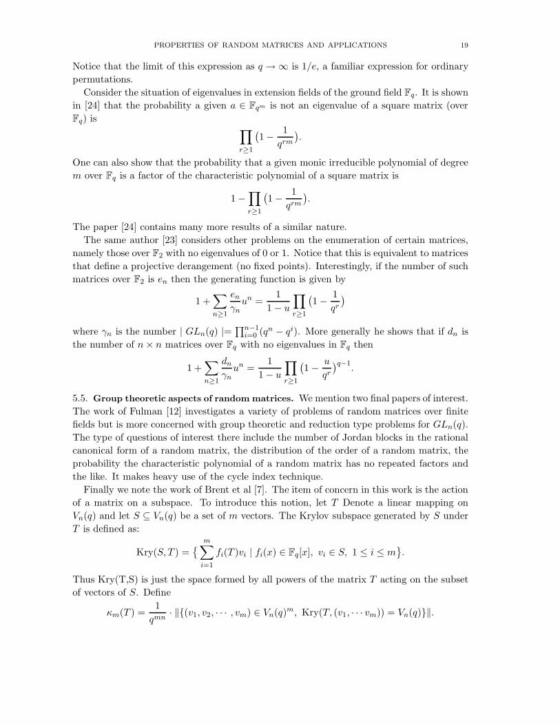
To begin, we confirm various results noted in Section 3, perhaps especially Theorem 3.2.
The following graphs consider the rank of (random binary) matrices where each element is
chosen at random and independently with probability p, as shown.
0
0.2
0.4
0.6
0.8
1
100 102 104 106 108 110
Pro
babi
lity
of F
ull R
ank
Number of Columns (k+m)
theoryp = 0.5p = 0.4p = 0.3p = 0.2p = 0.1
0
0.2
0.4
0.6
0.8
1
500 502 504 506 508 510
Pro
babi
lity
of F
ull R
ank
Number of Columns (k+m)
theoryp = 0.5p = 0.4p = 0.3p = 0.2p = 0.1
Figure 1. Probability of rank k for a k×(k+m) matrix. The left graph shows the
results for k = 100, while the right is for k = 500. In both graphs, the theoretical
expression of Equation 3.4 is shown versus experimental results for the probability
of a nonzero element p = 0.1, 0.2, 0.3, 0.4, 0.5. Each point of the experimental
results is for 50, 000 trials for k = 100 and 5, 000 trials for k = 500.
The agreement of experiment with theory, for p sufficiently large, in these graphs is quite
surprising. Further experiments for k down to 10 showed similar agreement. Note that all
values of p in these curves exceed the threshold value of ln(k)/k.
It was noted in Section 3 that a critical value for the probability p for choosing the
nonzero elements in a random matrix was p = ln k/k for a matrix with k rows. The following
experimental results attempt to justify this, showing the behavior of the probability of full
rank as p varies around log(k)/k. Additionally we show that the expression for Qm corrected
for the probability of zero rows and columns (Equation 6.1)is accurate well below this value,
although it becomes increasingly difficult to verify this experimentally.
Based on these experimental results and the expressions of the previous sections it can
be justified that the rank properties of a random matrix over F2 where the matrix elements
are chosen to be 1, independently and identically with probability p where 2 ln(k)/k <
p < 1 − 2 ln(k)/k, are indistinguishable from the purely random case where p = 1/2. For
example the expression equation (3.6) can be used to show this 1
Note that from the theorems of Section 3 the critical value of probability is p = ln(k)/k
and for a value of p slightly larger, asymptotically as k, m increase, the rank tends to full.
size of p needed to behave as a ”purely random” (p = 1/2) matrix is . Based on the work
of Kolchin and Cooper, the correct lower bound for the value of p in order for the rank
poprties of the matrix to be similar for the random (p = 1/2 case) is likely of the form
p = (ln(k) + d(k))/k for a function d(k) decreasing to 0 sufficiently slowly with k.
1The authors are grateful to Omran Ahmadi for pointing this out.
22 IAN F. BLAKE AND CHRIS STUDHOLME
0
0.2
0.4
0.6
0.8
1
100 110 120 130 140 150
Pro
babi
lity
of F
ull R
ank
Number of Columns (k+m)
c = 1.5c = 1.3c = 1.0c = 0.8
0
0.2
0.4
0.6
0.8
1
500 510 520 530 540 550
Pro
babi
lity
of F
ull R
ank
Number of Columns (k+m)
c = 1.5c = 1.3c = 1.0c = 0.8
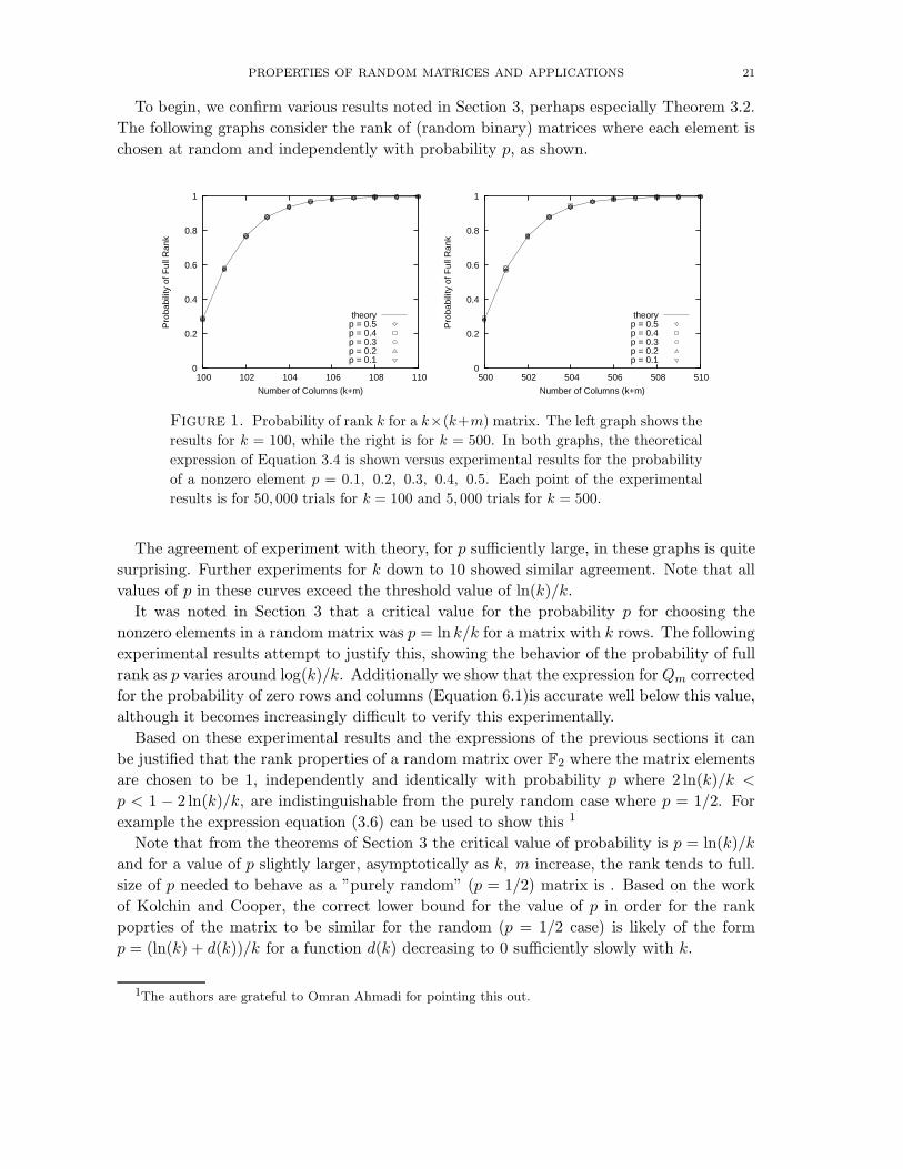
Figure 2. Probability of full rank for p = c ln(k)/k as the number of extra
columns increases. Each data point is the result of 50, 000 trials (for k = 100)
and 5, 000 trials (for k = 500). The solid line is computed using Equation
6.1 and the dotted line (purely random matrix with constant p > 2 ln(k)/k)
for Equation 3.4.
It has been observed the the average number of columns, beyond k, for a purely random
k× (k+m) to achieve full rank with high probability, is 1.60669515 · · · . Based on the above
observations, we suggest the following:
Conjecture 6.1. If the elements of a random binary k × (k + m) matrix Mk,(k+m) are
chosen independently and identically at random to be 1 with probability p, then the expected
number of columns beyond k required to achieve full rank (k), m, is, asymptotically as
k → ∞i) m = ∞ for p < ln(k)/k
ii) m = 1.60669515 · · · (as in section 3) for 2 ln(k)/k < p < 1 − 2 ln(k)/k
The behavior of m for p = c ln(k)/k for 1 < c < 2 would be of interest.
So far we have only considered generating columns for the random matrices by choosing
the individual column elements at random, identically and independently distributed. It is
interesting to consider other mechanisms to generate the columns and we will have a use
for one such mechanism when considering applications for the material to coding.
For the mechanism to be considered, assume we have a ”degree distribution” available,
p(d), d = 1, 2, · · · , k where p(d) is the probability of choosing a degree of d. The terminology
derives from coding theory where the binary matrix is viewed as a bipartite graph. The
process will be, for each column to be added to the random matrix, d is chosen according to
the distribution, and the column is formed by choosing a random d-tuple of integers from
1 to k to place the ones. For this we use the terms weight and degree interchangeably.
Several distributions are used.
Wedge distribution: To achieve a mean column weight of σ, which we assume is not of the
form of an integer plus 0.5, we choose degrees, d − 1, d, d + 1 where d is σ rounded to
the nearest integer. The probability assigned to d is 0.5 and the sum of probabilities for
d − 1, d + 1 is 0.5, with mean degree σ, resulting in a unique distribution.

PROPERTIES OF RANDOM MATRICES AND APPLICATIONS 23
0
0.2
0.4
0.6
0.8
1
100 110 120 130 140 150
Pro
babi
lity
of F
ull R
ank
Number of Columns (k+m)
c = 2.0c = 1.2c = 1.0
0
0.2
0.4
0.6
0.8
1
500 510 520 530 540 550
Pro
babi
lity
of F
ull R
ank
Number of Columns (k+m)
c = 2.0c = 1.2c = 1.0
Figure 3. Probability of rank k for a k × (k + m) matrix. The left graph shows
the results for k = 100, while the right is for k = 500. The graphs use p = c ln(k)/k
in Equation 6.1 and the data points are derived from the wedge distribution with
the same mean.
Uniform distribution: To achieve a mean degree (weight) of σ we assign probabilities of
approximately 1/2σ to degrees 1, 2, · · · , to approximately 2σ, adjusting the probability of
the last degree to achieve the correct mean.
0
0.2
0.4
0.6
0.8
1
100 110 120 130 140 150
Pro
babi
lity
of F
ull R
ank
Number of Columns (k+m)
c = 2.0c = 1.2c = 1.0
0
0.2
0.4
0.6
0.8
1
500 510 520 530 540 550
Pro
babi
lity
of F
ull R
ank
Number of Columns (k+m)
c = 2.0c = 1.2c = 1.0
Figure 4. Probability of rank k for a k × (k + m) matrix. The left graph shows
the results for k = 100, while the right is for k = 500. The graphs use p = c ln(k)/k
in Equation 6.1 and the data points are derived from the uniform distribution with
the same mean.
Horshoe distribution: Half of the columns have low degree (2 or 3) and half have high
degree (approximately 2σ). We used two variants: in the degree 2 variant, we used half
of the columns of weight 2 and the other half of weight d and d + 2, d odd, choosing the
probabilities to give the correct mean. In the degree 3 variant we choose half of the columns
of weight 3 and the other half of degrees d and d + 1 (note: a matrix with all columns of
even weight cannot have full rank and these considerations are to avoid this possibility).

24 IAN F. BLAKE AND CHRIS STUDHOLME
0
0.2
0.4
0.6
0.8
1
100 110 120 130 140 150
Pro
babi
lity
of F
ull R
ank
Number of Columns (k+m)
c = 2.0c = 1.2c = 1.0
0
0.2
0.4
0.6
0.8
1
500 510 520 530 540 550
Pro
babi
lity
of F
ull R
ank
Number of Columns (k+m)
c = 2.0c = 1.2c = 1.0
Figure 5. Probability of rank k for a k×(k+m) matrix. The left graph shows the
results for k = 100, while the right is for k = 500. The graphs use p = c ln(k)/k in
Equation 6.1 and the data points are derived from the horshoe distribution (variant
2) with the same mean.
0
0.2
0.4
0.6
0.8
1
100 110 120 130 140 150
Pro
babi
lity
of F
ull R
ank
Number of Columns (k+m)
c = 2.0c = 1.2c = 1.0
0
0.2
0.4
0.6
0.8
1
500 510 520 530 540 550
Pro
babi
lity
of F
ull R
ank
Number of Columns (k+m)
c = 2.0c = 1.2c = 1.0
Figure 6. Probability of rank k for a k×(k+m) matrix. The left graph shows the
results for k = 100, while the right is for k = 500. The graphs use p = c ln(k)/k in
Equation 6.1 and the data points are derived from the horshoe distribution (variant
3) with the same mean.
Soliton distribution: This distribution will be of interest in the coding section (Section 7).
The distribution is given by
p(d) =
1/k i = 1
1/i(i − 1) 2 ≤ i ≤ k.
It is seen there is very little difference in the results of the wedge, uniform and horshoe
distributions for the same mean column weight. As far as rank properties of the random
matrices are concerned, as long as the mean column weights are the same, one can either
choose the column elements at random with probability p or choose the column weight d
from the distribution and then a random d-tuple from [1, k].
However for the soliton distribution the results are significantly different (see Graph 7).
No explanation was found for this.

PROPERTIES OF RANDOM MATRICES AND APPLICATIONS 25
0
0.2
0.4
0.6
0.8
1
100 105 110 115 120 125 130
Pro
babi
lity
of F
ull R
ank
Number of Columns (k+m)
c = 1.3c = 1.1264
c = 1.0soliton
0
0.2
0.4
0.6
0.8
1
500 505 510 515 520 525 530
Pro
babi
lity
of F
ull R
ank
Number of Columns (k+m)
c = 1.3c = 1.093
c = 1.0soliton
Figure 7. Probability of rank k for a k × (k + m) matrix. The left graph shows
the results for k = 100, while the right is for k = 500. The graphs use p = c ln(k)/k
in Equation 6.1 and the data points are derived from the soliton distribution with
similar mean. Note for k = 100 the mean of the soliton distribution is approximately
1.1264 ln(k) and for k = 500 it is approximately 1.093 ln(k)/k.
Experiments for the windowed matrices described in Section 5.1 are considered.
0
0.2
0.4
0.6
0.8
1
100 102 104 106 108 110
Number of Columns (k+m)
theoryrandom
w=20w=15w=10
0
0.2
0.4
0.6
0.8
1
900 902 904 906 908 910
Number of Columns (k+m)
theoryw=60w=45w=30
Figure 8. Probability of rank k for a k × (k + m) matrix. The left graph shows
the results for k = 100, while the right is for k = 900. In both graphs, the dotted
line is Qm (Equation 3.4), the open circles show results from random (p = 1/2) ma-
trices, and the other symbols show results for windowed matrices (with the specified
window size). For clarity, no open circles are shown on the right graph.
The curves of Graph 8 (and subsequent graphs) suggest the lower bound of 2√
k for full
rank falls slightly short for lower values of k (≤ 100) but appears quite accurate for larger
values, in terms of obtaining rank behaviour of the windowed matrices equivalent to those
of a random matrix.
The Graph 10 is similar to previous curves with slightly extended horizontal range.
The conclusions of this experimental evidence suggests that windowed matrices with
window size at least w ≥ 2√
k with mean column weight higher then 2 ln(k) give probabilities
of full rank as those of purely random matrices, but that otherwise the effect of window
size beyond 2√
k has little effect.

26 IAN F. BLAKE AND CHRIS STUDHOLME
0
0.2
0.4
0.6
0.8
1
2500 2502 2504 2506 2508 2510
Number of Columns (k+m)
theoryw=100
low weightw=75w=50
0
0.2
0.4
0.6
0.8
1
10000 10002 10004 10006 10008 10010
Number of Columns (k+m)
theoryw=200
low weightw=150w=100
Figure 9. Probability of rank k for a k × (k + m) matrix. The left graph shows
the results for k = 2500, while the right is for k = 10000. In both graphs, the broken
line is Qm (Equation 3.4), the open triangles show results for random (p = 1/2)
matrices (window size 2√
k, 100 and 200 respectively), and the other symbols show
results for windowed matrices (with the specified window size). The low weight
closed triangles are the results for a window size of w = 2√
k but with the mean
column weight fixed at 2 log k.
0
0.2
0.4
0.6
0.8
1
100 105 110 115 120
Pro
babi
lity
of F
ull R
ank
Number of Columns (k+m)
Probability of Full Rank (k=100)
window length = 20window length = 15window length = 10
0
0.2
0.4
0.6
0.8
1
10000 10005 10010 10015 10020
Pro
babi
lity
of F
ull R
ank
Number of Columns (k+m)
Probability of Full Rank (k=10000)
window length = 200window length = 150window length = 100
Figure 10. Probability of rank k for a k × (k + m) matrix. The left graph shows
the results for k = 100, while the right is for k = 10000. In both graphs, the broken
line is Qm, and the other symbols show results for windowed matrices (with the
specified window size), for p = 1/2 within a window.
The remaining graphs are given without caption and are self explanatory, where the
termforced start refers to the first (topmost element) in the window is forced to be 1.
Curves where the probability of a nonzero element is chosen to make the mean column
weight 2 ln(k) are so marked. All other curves use p = 1/2. The dotted curve in each graph
is Equation 3.4.
Conjecture 6.2. The rank properties of a binary windowed k × (k + m) random matrix,
as discussed in section 5.1, behave as a random binary matrix iff the window length is at
least 2√
k as long as the probability of an element being 1 is at least p, where p is chosen to
give a mean column weight of 2 ln(k).

PROPERTIES OF RANDOM MATRICES AND APPLICATIONS 27
0
0.2
0.4
0.6
0.8
1
100 105 110 115 120
Pro
babi
lity
of F
ull R
ank
Number of Columns (k+m)
Probability of Full Rank (k=100; forced start)
window length = 20window length = 15window length = 10
0
0.2
0.4
0.6
0.8
1
100 105 110 115 120
Pro
babi
lity
of F
ull R
ank
Number of Columns (k+m)
Probability of Full Rank (k=100; weight 2 log k)
window length = 20window length = 15window length = 10
Figure 11. Probability of rank k for a k × (k + m) matrix for k = 100. In
both graphs, the broken line is Qm: the left graph shows results for random (p =
1/2) (windowed, forced start) matrices, and the other show results for low weight
windowed matrices.Note low value of k here.
0
0.2
0.4
0.6
0.8
1
900 905 910 915 920
Pro
babi
lity
of F
ull R
ank
Number of Columns (k+m)
Probability of Full Rank (k=900; forced start)
window length = 60window length = 45window length = 30
0
0.2
0.4
0.6
0.8
1
900 905 910 915 920
Pro
babi
lity
of F
ull R
ank
Number of Columns (k+m)
Probability of Full Rank (k=900; weight 2 log k)
window length = 60window length = 45window length = 30
Figure 12. Probability of rank k for a k × (k + m) matrix. Similar to previous
graphs only for k = 900. In both graphs, the broken line is Qm. The left graph
shows results for random (p = 1/2) and forced start matrices, and the right for low
weight.
We conclude the section with some experimental results associated with the work of
Calkin [8] on random matrices with constant weight columns and to verify the behaviour
of the threshold of βk mentioned there.
28 IAN F. BLAKE AND CHRIS STUDHOLME
0
0.2
0.4
0.6
0.8
1
2500 2505 2510 2515 2520
Pro
babi
lity
of F
ull R
ank
Number of Columns (k+m)
Probability of Full Rank (k=2500; forced start)
window length = 100window length = 75window length = 50
0
0.2
0.4
0.6
0.8
1
2500 2505 2510 2515 2520
Pro
babi
lity
of F
ull R
ank
Number of Columns (k+m)
Probability of Full Rank (k=2500; weight 2 log k)
window length = 100window length = 75window length = 50
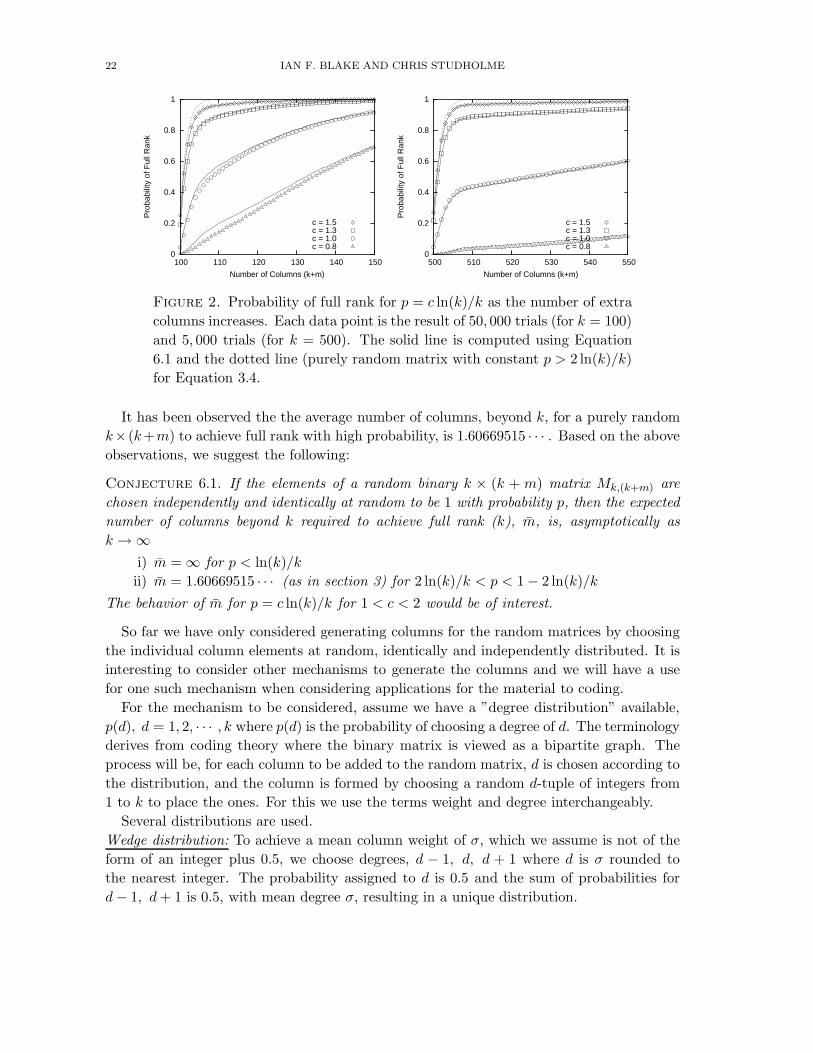
Figure 13. Probability of rank k for a k × (k + m) matrix. Similar to previous
graphs only for k = 2500. In both graphs, the broken line is Qm. The left graph
shows results for random (p = 1/2) and forced start matrices, and the right for low
weight.
0
0.2
0.4
0.6
0.8
1
2500 2505 2510 2515 2520
Pro
babi
lity
of F
ull R
ank
Number of Columns (k+m)
Probability of Full Rank (k=2500; weight 3 log k)
window length = 100window length = 75window length = 50
0
0.2
0.4
0.6
0.8
1
2500 2505 2510 2515 2520
Pro
babi
lity
of F
ull R
ank
Number of Columns (k+m)
Probability of Full Rank (k=2500; weight 4 log k)
window length = 100window length = 75window length = 50
Figure 14. Probability of rank k for a k × (k + m) matrix. Similar to previous
graphs with k = 2500 and higher mean column weight. In both graphs, the broken
line is Qm.
k n = 500 n = 1000 n = 2000 theory3 theory2
2 0.464 < b < 0.466 0.459 < b < 0.460 0.4563 < b < 0.4577
3 0.914 < b < 0.916 0.916 < b < 0.917 0.9170 < b < 0.9175 0.90912 0.92817
4 0.972 < b < 0.974 0.974 < b < 0.975 0.9755 < b < 0.9760 0.96909 0.97358
5 0.990 < b < 0.992 0.991 < b < 0.992 0.9920 < b < 0.9925 0.98935 0.99028
6 0.992 < b < 0.994 0.995 < b < 0.996 0.9960 < b < 0.9965 0.99625 0.99642
7 0.996 < b < 0.998 0.998 < b < 0.999 0.9985 < b < 0.9990 0.99865 0.99868
8 0.9985 < b < 0.9990 0.99951 0.99952
9 0.9995 < b < 0.9999 0.99982 0.99982

PROPERTIES OF RANDOM MATRICES AND APPLICATIONS 29
0
0.2
0.4
0.6
0.8
1
10000 10005 10010 10015 10020
Pro
babi
lity
of F
ull R
ank
Number of Columns (k+m)
Probability of Full Rank (k=10000; forced start)
window length = 200window length = 150window length = 100
0
0.2
0.4
0.6
0.8
1
10000 10005 10010 10015 10020
Pro
babi
lity
of F
ull R
ank
Number of Columns (k+m)
Probability of Full Rank (k=10000; weight 2 log k)
window length = 200window length = 150window length = 100
Figure 15. Probability of rank k for a k × (k + m) matrix. Similar to previous
graphs with k = 10000 and mean column weight as indicated. In both graphs, the
broken line is Qm.
0
0.2
0.4
0.6
0.8
1
10000 10005 10010 10015 10020
Pro
babi
lity
of F
ull R
ank
Number of Columns (k+m)
Probability of Full Rank (k=10000; weight 4 log k)
window length = 200window length = 150window length = 100
Figure 16. Probability of rank k for a k × (k + m) matrix. Similar to previous
graphs with k = 10000 and higher mean column weight as indicated. The broken
line is Qm.
In this table, the column labelled ‘theory3’ is the 3 term expression for βk mid way down
on page 270 of [8] and ‘theory2’ is the approximation βk ∼ 1− exp(−k)/log(2). The ranges
of values shown in columns 2 to 5 were extracted from the graph 17 below. It proved a very
difficult problem to assess these values with accuracy.
For the probabilty of independence (full rank) in the square case:
k n=500 n=1000 n=2000
3 0 0 0
5 0.007694 0.00012 0
7 0.183832 0.11501 0.0460
9 0.271318 0.25741 0.2316
11 0.2836
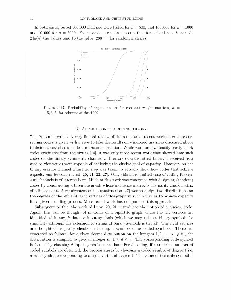
30 IAN F. BLAKE AND CHRIS STUDHOLME
In both cases, tested 500,000 matrices were tested for n = 500, and 100, 000 for n = 1000
and 10, 000 for n = 2000. From previous results it seems that for a fixed n as k exceeds
2 ln(n) the values tend to the value .288 · · · for random matrices.
0
0.2
0.4
0.6
0.8
1
950 960 970 980 990 1000
Pro
babi
lity
of D
epen
dent
Set
Number of Columns
Probability of Dependent Set (n=1000)
4567
Figure 17. Probability of dependent set for constant weight matrices, k =
4, 5, 6, 7. for columns of size 1000
7. Applications to coding theory
7.1. Previous work. A very limited review of the remarkable recent work on erasure cor-
recting codes is given with a view to take the results on windowed matrices discussed above
to define a new class of codes for erasure correction. While work on low density parity check
codes originates from the sixties [14], it was only more recent work that showed how such
codes on the binary symmetric channel with errors (a transmitted binary 1 received as a
zero or vice-versa) were capable of achieving the elusive goal of capacity. However, on the
binary erasure channel a further step was taken to actually show how codes that achieve
capacity can be constructed [20, 21, 22, 27]. Only this more limited case of coding for era-
sure channels is of interest here. Much of this work was concerned with designing (random)
codes by constructing a bipartite graph whose incidence matrix is the parity check matrix
of a linear code. A requirement of the construction [27] was to design two distributions on
the degrees of the left and right vertices of this graph in such a way as to achieve capacity
for a given decoding process. More recent work has not pursued this approach.
Subsequent to this, the work of Luby [20, 21] introduced the notion of a rateless code.
Again, this can be thought of in terms of a bipartite graph where the left vertices are
identified with, say, k data or input symbols (which we may take as binary symbols for
simplicity although the extension to strings of binary symbols is trivial). The right vertices
are thought of as parity checks on the input symbols or as coded symbols. These are
generated as follows: for a given degree distribution on the integers 1, 2, · · · , k, ρ(k), the
distribution is sampled to give an integer d, 1 ≤ d ≤ k. The corresponding code symbol
is formed by choosing d input symbols at random. For decoding, if a sufficient number of
coded symbols are obtained, the process starts by choosing a coded symbol of degree 1 i.e.
a code symbol corresponding to a right vertex of degree 1. The value of the code symbol is

PROPERTIES OF RANDOM MATRICES AND APPLICATIONS 31
transferred to the corresponding input symbol, whose value is then transferred to all coded
symbols containing it, and all the corresponding edges are removed from the graph. If a
new right vertex is now of degree 1, the process continues.
Clearly the decoding continues until it completes with all input symbols recovered or
there are no right vertices of degree 1 at some stage, in which case the decoding fails.
To minimize the probability of the latter, the distribution ρ(i) is chosen carefully. Ini-
tially, it was suggested [21] to use the soliton distribution given by ρ(i) = 1/i(i − 1), i =
2, 3, · · · , k, ρ(1) = 1/k. The theoretical reasoning for this distribution is sound, but it turns
out in practice that the probability, at each stage of the decoding, of having a vertex of
degree 1 is too sensitive, giving too high a probability the decoding would not complete. To
remedy the situation, a robust soliton distribution was suggested that proved more robust
in practice. These codes are referred to as rateless since the decoder can continue to gather
coded symbols from any source, on the same input data, until decoding completes – there
is no fixed a priori rate associated with the code. In conventional coding, it would first be
necessary to estimate the erasure probability to allow proper code design and this rateless
feature is very useful.
For an original set of k data or input symbols, the number of extra (more than k) coded
symbols required to give a high probability of decoding completion is referred to as the
overhead. It is shown in [21] that if δ is the allowable decoding failure probability then by
using the robust soliton distribution for the generation of the coded symbols, the overhead
required to decode is k + O(√
k ln2(k/δ)) and the average degree of the right vertices is
D = ln(k/δ). Since the complexity of decoding is proportional to the number of edges in
the graph, this last result shows the decoding complexity to be O(k ln(k/δ)).
To improve the situation further Shokrollahi [27] and independently Maymounkov [22]
introduced the idea of precoding. Here one uses a good erasure correcting code to code the
original input symbols resulting in a certain number of auxiliary symbols. These are then
added to the input symbols (on the left hand side of the bipartite graph) and the combined
set of left hand side symbols are coded using a truncated soliton-like encoder. This latter
(outer) code has a mean right hand side degree that is independent of k, giving linear time
encoding and decoding. In exchange for this complexity reduction, overhead is increased
to O(k) extra coded symbols. For convenience, we note Theorem 2 from [22], using our
terminology. A similar result is found in [27, 11].
Theorem 7.1. (Maymounkov): For any message of size k input symbols, and any param-
eter ǫ > 0, there is a rateless locally encodable code (right distribution) that can recover the
input symbols from any (1 + ǫ)k coded symbols with high probability in time proportional to
k log(1/ǫ).
100%
10%
1%
0.1% 10 100 1000 10000
Number of Input Symbols (k)Figure 18. Mean over-
In the presence of such a powerful result one
might wonder why further work on this problem
might be of interest. One aspect of the above is
that they are essentially asymptotic results. In
practice, with our simulations and others avail-
able in the references, a typical overhead for the

32 IAN F. BLAKE AND CHRIS STUDHOLME
LT decoding might be as much as 15% for a num-
ber of input symbols on the order of a thousand
and this drops to perhaps 3% to 4% for a much
higher number of input symbols. The Online or
Raptor codes can be constructed to have an over-
head of 3% to 4%, of k for large k. For an idea of
the improvement in overhead that is possible, see
figure 18. The solid line in this figure illustrates
the overhead achievable by our erasure code con-
struction which we take as approximately 2 sym-
bols, independent of k.
The class of codes presented here will have a
decoding complexity of O(k3/2) for k input sym-
bols. Although significantly higher than the previous work, for low k the increase is not
so large when all the constants in the estimates are taken into account. In return for this
increased complexity, one obtains codes that are effective for values of k as low as 100, are
easily generated requiring only a uniform distribution, and have a very high and quantifiable
probability of decoding completion with an overhead that is constant, independent of k. It
is likely there will be applications where such properties are of interest.
7.2. Erasure code construction. In this section we describe how one might use these
windowed random matrices to construct an efficiently encodable and decodable erasure
code.
7.2.1. Encoding. The encoder begins with the k data symbols (input blocks) that need to be
transmitted. From these input blocks, the encoder generates, randomly and independently,
columns of a windowed matrix along with output data blocks (coded symbols). There is
one output block associated with each column.
Here are the steps the encoder takes to generate an output data block:
(1) Choose a starting row number (uniformly) within the range 1, . . . , k.
(2) For each of the w rows starting at this start row, decide whether a 1 or a 0 will be
placed in that row. These two choices may be equally likely, or not (see below).
(3) For each 1 in the column generated in step 2, sum the corresponding input blocks
using bitwise exclusive or.
(4) Send the column and output block (sum) to the decoder.
In this last step, sending the column need not require O (k), or even O(√
k) space. Instead,
one might send a small seed for a pseudo-random number generator that is used by both
parties to generate the column. This requires O (log k) space.
With w = 2√
k, the maximum number of input blocks to be summed is w. For a densely
packed window, the expected number is w/2 =√
k; however, we can do better than this.
In figure 11, right graph, the closed triangles give the probability of full rank for w = 2√
k
but with a mean column weight of 2 log k. Note that these results are almost as good as the
results for a densely packed window, and therefore, if one wishes to reduce the per output
block encoding time to O (log k), one can modify step 2 to instead choose 2 log k 1’s within

PROPERTIES OF RANDOM MATRICES AND APPLICATIONS 33
the window chosen in step 1. Be careful, however, to ensure that it is not the case that
every column has even weight. Such a matrix will be singular. Perhaps choose the next
largest odd integer greater than 2 log k and generate columns with that weight.
7.2.2. Avoiding Wrapping. In the next section, while discussing the decoding algorithm,
we will notice that the decoder must treat columns that wrap from bottom to top as though
they have length k. We will also see that these long length columns can increase the work
to be done by the decoder by a factor of 2. Therefore, to avoid this extra work, we have
developed a strategy to avoid columns that wrap; however, as we will see, this strategy may
not reduce the work to be done by the decoder as much as we would like.
The strategy involves both a non-uniform distribution on the starting row selection (step
1 above) and a variable window length. The calculations required are all based on the
binomial theorem and are similar to those of previous theorems. Unfortunately, we find
that, to achieve a probability of full rank that is similar to what we see when wrapping is
allowed, the required window length for columns with an initial 1 near the middle of the
column is about 4√
k, and the mean window length is a little greater than 3√
k. This negates
much of the benefit of avoiding wrapping. Regardless, we will give a complete description
of the non-wrapping encoder and a detailed performance comparison in the full version of
this paper.
7.3. Decoding. The decoding algorithm is simply Gaussian Elimination; however, to en-
sure our discussion of decoder complexity is precise, we will describe a specific decoding
algorithm. Decoding has two phases:
(1) Column collection. During column collection, matrix columns, along with their
associated data blocks, are inserted into a hash table and reduced as necessary to
ensure they are independent.
(2) Back filling. At the conclusion of column collection, we will have a lower triangular
matrix with 1’s along the diagonal. This matrix is non-singular. With a series of
data block sums, the matrix is essentially made diagonal and decoding is complete.
The hash table constructed during the first phase is to have exactly k bins. Each column
received hashes to the bin whose index is the index of the first row containing a 1. When
this table is full, we will have k columns, all of which start at a different row (ie. a lower
triangular matrix with 1’s along the diagonal). For the purposes of this algorithm, we do
not consider any columns to wrap from bottom to top, and as a result, the first 1 in a
column may not coincide with the start of the window.
During column collection, we will occasionally come across two columns whose initial
1’s are in the same row. This is a hash collision and requires collision resolution. Such
resolution is easy, simply add the two columns (and their associated data blocks) together.
The resulting column is guaranteed not to have it’s initial 1 in the same row. A subtle but
important aspect of this algorithm is the choice of columns to keep after collision resolution.
Obviously, the sum is to be kept. The other column to keep is the shorter of the two colliding
columns. Here, the length of a column is the number of rows between the first 1 and the
last 1 (inclusive). If the two columns are of equal length, either one may be kept.
34 IAN F. BLAKE AND CHRIS STUDHOLME
It may also happen during collision resolution that the two colliding columns are identical
and their sum is the all zero column. In this case, one of the two columns is simply discarded
and an extra column must be collected.
When the hash table is full, back filling can begin. Back filling is done starting at the
last row and working up through the matrix. First, the data block associated with the 1
on the diagonal is added to all of the data blocks associated with 1’s in the last row. Then,
the second to last row is processed in a similar manner. At the completion of back filling,
the data blocks will be the original input blocks.
Theorem 7.2. Worst case decoder complexity is lk data block additions, where l is the
mean column length. Column length, l, as mentioned earlier in this section, is the number
of rows between the first 1 and the last 1, inclusive.
Proof. During the column collection phase, one data block addition is required each time
there is a hash table collision. If two columns, one of length x and the other of length y,
x ≤ y, collide, their sum will be a column whose length is no greater than y − 1. Since lk
is the sum of the length’s of the columns and each collision reduces this total length by at
least 1, there can be at most lk collisions.
During the back filling phase, the number of data block additions needed is exactly the
weight of the matrix (after column collection) less k. Also, the weight of the matrix is no
greater than the total length, and the total length after column collection no greater than
the total length before column collection less the number of collisions. Therefore, the sum
of the weight of the matrix after column collection and the number of collisions resolved
during column collection is at most lk.
The average case complexity is lk/2. This is easily seen by noting that when columns of
length x and y, x ≤ y, are added, the expected length of the resulting column is at most
y − 2. Furthermore, the expected weight of the matrix after column collection is half the
total length.
To see how the average case complexity may be calculated from w, first notice that for
columns that do not wrap, l ≤ w; however, for columns that do wrap, l may be as large as
k. In the case where wrapping is allowed, we suggest w = 2√
k is sufficient to achieve low
overhead. Note that the probability of generating a column that wraps is w/k. This means
that, after k columns have been generated, we only expect w of them to wrap. The mean
column length (as seen by the decoder) is thus l = wk + (k −w)w ≈ 2wk. This gives us an
average case decoder complexity of wk = 2k3/2.
It was suggested earlier that we may be able to avoid generating columns that wrap;
however, in doing so columns with a window length as large as 4√
k may be generated.
This means l may be as large as 4√
k and thus decoder complexity is still 2k3/2. Actually,
in this no-wrapping case, l is closer to 3√
k so there may yet be a benefit to avoiding
wrapping.
7.4. Conclusions. An efficiently encodable and decodable class of erasure correcting codes,
with decoding complexity O(k3/2), based on the rank properties of windowed binary random
matrices, has been formulated. They have the advantages over other classes of erasure

PROPERTIES OF RANDOM MATRICES AND APPLICATIONS 35
correcting codes of a low and fixed overhead and effectiveness at much lower block lengths.
The necessity of the rank properties required for the windowed matrices are established
here. While simulation and intuitive arguments show the conditions needed are clearly
sufficient it is hoped to establish these properties analytically in future work.
8. A diversion
There are numerous applications of the matrices considered here as well as many other
related problems, including combinatorics, coding, theoretical computer science etc.. We
mention a problem that has been of interest in computer science, that of the singularity of
random (equally likely) ±1 matrices taken over the integers (or rationals). (Recall, the work
of this report has been concerned exclusively with rank over the finite field of interest.) Let
Mn be an n × n random ±1 matrix. It long been conjectured that
P (det(Mn) = 0) ≥ (1 + o(1))n221−n,
a result of the fact that such a random matrix with two identical or opposite columns
has a determinant of 0, which has also been conjectured as the main source of singularity.
However the best actual result in this direction is:
Theorem 8.1.
P (det(Mn) = 0) = O((1 − ǫ)n)
where [15] ǫ = .001 improved to ǫ = .0691 · · · [28].
(The constant ǫ = .0691 · · · in the theorem is the unique solution to the equation
h(ǫ) + ǫ/(log2(16/15)) = 1
in the interval (0, 1/2), where h(·) is the binary entropy function.) It is also noted there
([28]) that from Hadamard’s inequality we have that
det(Mn) ≤ nn/2
with equality iff Mn is a Hadamard matrix. Furthermore it can be shown that
E((det Mn)2) = n!
and higher moments are also computable. A main result of [28] is that
P (det(Mn) = ±√
n! exp(−o(n1/2+ǫ)) =1
2− o(1).
It is interesting, although not surprising, that the behavior of this case is so different than
the binary 0, 1 over F2.
9. Comments
A very brief overview of certain aspects of rank properties of random matrices over finite
fields has been considered and certain questions of interest have been posed. It has been
intended only as a document for possible use in pursuing further work in the area.
Acknowledgements: The authors would like to thank Igor Shparlinski for his careful
reading of the report and suggestions for improvement.

36 IAN F. BLAKE AND CHRIS STUDHOLME
References
1. G.V. Balakin, The disribution of the rank of random matrices over a finite field, Theory Prob. Appl.,,
vol. 8, no. 4, pp. 594-605, 1968.
2. E.R. Berlekamp, The technology of error correcting codes, Proc. IEEE, vol. 68, pp. 564-593, 1980.
3. C. Bertram-Kretzberg, T. Hofmeister and H. Lefmann, Sparse 0−1 matrices and forbidden hypergraphs,
Combinatorics, Probability and Computing, vol. 8, pp. 417-427, 1999.
4. Ian F. Blake and Ronald C. Mullin, The Mathematical Theory of Coding, Academic Press, 1975.
5. Johannes Blomer and Richard Karp and Emo Welzl, The rank of sparse random matrices over finite
fields, Random Structures and algorithms, vol. 10, pp 407–419, 1997.
6. Bela Bollobas, Random Graphs, 2nd edition, Cambridge, 2001.
7. R. Brent, S. Gao and A. Lauder, Random Krylov spaces over finite fields, SIAM J. Discrete Math., vol.
16, pp. 276–287, 2003.
8. N. Calkin, Dependent sets of constant weight binary vectors, Combinatorics, Probability and Computing,
vol. 6, pp. 263-271, 1997.
9. C. Cooper, On the rank of random matrices, Random Structures and Algorithms, vol. 16, no. 2, pp.
209-232, 2000.
10. C. Cooper, On the distribution of rank of a random matrix over a finite field, Random Structures and
Algorithms, vol. 17, pp. 197-212, 2000.
11. O. Elesami and A. Shokrollahi, Raptor codes on binary memoryless symmetric channels, IEEE Trans.
Information Theory, vol. 52, pp. 2033-2051, 2006.
12. J. Fulman, Random matrix theory over finite fields, Bull. Amer. Math. Soc., vol. 39, no. 1, pp. 51-85,
2001.
13. R. Sedgewick and P. Flajolet, Analysis of Algorithms, Addison-Wesley, 1996.
14. R.G. Gallager, Low Density Parity Check Codes, MIT Press, 1963.
15. J. Kahn, J. Komlos and E. Szemeredi, On the probability that a random ±1 matrix is singular, J.
American Math. Society, vol. 8, no. 1, pp. 223-240, 1995.
16. V.F. Kolchin, Random Graphs, Cambridge, 1999.
17. G. Landsburg, Uber eine Anzahlbestimmiung und eine damit zusammenhangende Reihe, J. Reine
Angew. Math. vol. 111, pp. 87-88, 1893.
18. H. Lefmann, P. Pudlick and P. Savicky, On sparse parity check matrices, Designs, Codes and Cryptog-
raphy, vol. 12, pp. 107-130, 1997.
19. H. Lefmann, Sparse parity check matrices over finite fields, COCOON 2003, T. Warnow and B. Zhu
eds., LNCS vol. 2697, pp. 112-121, 2003.
20. Michael Luby, Michael Mitzenmacher, M. Amin Shokrollahi, Daniel Speilman and Volker Stemann,
Practical loss-resilient codes, STOC, pp. 150–159, 1997.
21. M. Luby, LT codes, 43rd FOCS, pp. 271-280, 2002.
22. P. Maymounkov, Online Codes, Technical Report TR2002-833, New York University, October 2002.
23. Kent Morrison, Eigenvalues of random matrices over finite fields, preprint, 1999.
24. Kent Morrison, Matrices over Fq with no eigenvalues of 0 or 1, preprint, 2004.
25. A. Mukhopadhyay, The probability that the determinant of an n× n matrix over a finite field vanishes,
Discrete Mathematics, vol 51, pp. 311-315, 1995.
26. Assaf Naor and Jacques Verstraete, Improved bounds on the size of sparse parity check matrices, preprint,
2005.
27. A. Shokrollahi, Raptor codes, IEEE Trans. Information Theory, vol. 52, pp. 2551-2567, 2006.
28. T. Tao and Van Wu, On random ±1 matrices: Singularity and determinant, STOC 2005, pp. 431-440.
(Also, Random Structures and Algorithms, vol. 28, no. 4, pp. 1-23, 2005).
29. J.H. van Lint and R.M. Wilson, A Course in Combinatorics, Cambridge, 1992.

PROPERTIES OF RANDOM MATRICES AND APPLICATIONS 37
Department of Electrical and Computer Engineering, University of Toronto, Toronto,
Ontario M5S 3G4
E-mail address: [email protected]
Department of Computer Science, University of Toronto, Toronto, Ontario M5S 3G4
E-mail address: cvs@cs,utoronto.ca


![Operator-Valued Matrices with Free or Exchangeable Entries€¦ · As applications, we consider random matrices with independent blocks, as in [11], and random matrices in which the](https://static.fdocuments.us/doc/165x107/6059fdb7840fc35b3c17bce1/operator-valued-matrices-with-free-or-exchangeable-entries-as-applications-we-consider.jpg)