Properties of ﬂat-spectrum radio-loud narrow-line Seyfert ...

arX

iv:1

409.

3716

v4 [

astr

o-ph

.HE

] 8

Nov

201

9Astronomy & Astrophysics manuscript no. foschiniREV4 c©ESO 2019November 11, 2019

Properties of flat-spectrum radio-loud

narrow-line Seyfert 1 galaxies

L. Foschini1, M. Berton2, A. Caccianiga1, S. Ciroi2, V. Cracco2, B. M. Peterson3, E. Angelakis4, V. Braito1,L. Fuhrmann4, L. Gallo5, D. Grupe6, 7, E. Järvelä8, 9, S. Kaufmann10, S. Komossa4, Y. Y. Kovalev11, 4,

A. Lähteenmäki8, 9, M. M. Lisakov11, M. L. Lister12, S. Mathur3, J. L. Richards12, P. Romano13, A. Sievers14,G. Tagliaferri1, J. Tammi8, O. Tibolla15, 16, 17, M. Tornikoski8, S. Vercellone13 , G. La Mura2, L. Maraschi1, P. Rafanelli2

(Affiliations can be found after the references)

Received —; accepted —

ABSTRACT

We have conducted a multiwavelength survey of 42 radio loud narrow-1ine Seyfert 1 galaxies (RLNLS1s), selected by searchingamong all the known sources of this type and omitting those with steep radio spectra. We analyse data from radio frequencies toX-rays, and supplement these with information available from online catalogues and the literature in order to cover the full electro-magnetic spectrum. This is the largest known multiwavelength survey for this type of source. We detected 90% of the sources inX-rays and found 17% at γ rays. Extreme variability at high energies was also found, down to timescales as short as hours. In somesources, dramatic spectral and flux changes suggest interplay between a relativistic jet and the accretion disk. The estimated massesof the central black holes are in the range ∼ 106−8 M⊙, lower than those of blazars, while the accretion luminosities span a range from∼ 0.01 to ∼ 0.49 times the Eddington limit, similar to those of quasars. The distribution of the calculated jet power spans a rangefrom ∼ 1042.6 to ∼ 1045.6 erg s−1, generally lower than quasars and BL Lac objects, but partially overlapping with the latter. Oncenormalised by the mass of the central black holes, the jet power of the three types of active galactic nuclei are consistent with eachother, indicating that the jets are similar and the observational differences are due to scaling factors. Despite the observational differ-ences, the central engine of RLNLS1s is apparently quite similar to that of blazars. The historical difficulties in finding radio-loudnarrow-line Seyfert 1 galaxies might be due to their low power and to intermittent jet activity.

Key words. galaxies: Seyfert – galaxies: jets – quasars: general – BL Lacertae objects: general

1. Introduction

An important new discovery made with the Large Area Tele-scope (LAT, Atwood et al. 2009) on board the Fermi Gamma-raySpace Telescope (hereafter Fermi) is the high-energy gamma-ray emission from radio-loud narrow-line Seyfert 1 galaxies(RLNLS1s, Abdo et al. 2009a,b,c, Foschini et al. 2010).Narrow-line Seyfert 1 galaxies (NLS1s) are a well-known classof active galactic nuclei (AGNs), but they are usually consid-ered to be radio-quiet (e.g. Ulvestad et al. 1995, Moran 2000,Boroson 2002). Thus, the first discoveries of RLNLS1s (e.g.Remillard et al. 1986, Grupe et al. 2000, Oshlack et al. 2001,Zhou et al. 2003) seemed to be exceptions, rather than the tip ofan iceberg. The early surveys revealed only a handful of objects:11 by Zhou & Wang (2002) and Komossa et al. (2006a), and16 by Whalen et al. (2006). Williams et al. (2002) analysed 150NLS1s from the Sloan Digital Sky Survey (SDSS) Early Data Re-lease, and only a dozen (8%) were detected at radio frequenciesand only two (1.3%) are radio loud, i.e. with the ratio betweenradio and optical flux densities greater than 10. One source isalso in the present sample (J0948 + 0022, Zhou et al. 2003),while we have discarded the other (J1722+5654, Komossa et al.2006b) because of its steep radio index (see Sect. 2). Most of themildly radio-loud NLS1 galaxies of Komossa et al. (2006a) aresteep-spectrum sources, and do not show indications of beaming,while three sources are more similar to blazars. In terms of theiroptical emission-line properties and BH masses, the RLNLS1s

are similar to the radio-quiet NLS1 (RQNLS1) population as awhole. A larger study by Zhou et al. (2006) based on SDSSData Release 3 resulted in a sample of 2011 NLS1s, about 14%of all the AGNs with broad emission lines. The fraction detectedin the radio is 7.1%, similar to what was found by Williams etal. (2002). From this subsample, Yuan et al. (2008) culled 23RLNLS1s with radio loudness greater than 100 and found thatthese sources are characterised by flat radio spectra. Detectionof flux and spectral variability and their characteristic spectralenergy distributions (SEDs) suggest a blazar-like nature.

In 2009, detection at high-energy γ rays by Abdo et al.(2009a,c) revealed beyond any reasonable doubt the existenceof powerful relativistic jets in RLNLS1s and brought this poorlyknown class of AGNs into the spotlight (see Foschini 2012a fora recent review). An early survey including gamma-ray detec-tions (after 30 months of Fermi operations) was carried out byFoschini (2011a). Forty-six RLNLS1s were found, of whichseven were detected by Fermi. Of 30 RQNLS1 that served asa control sample, none were detected at γ rays. Additional mul-tiwavelength (MW) data, mostly from archives, were employedin this survey; specifically, X-ray data from ROSAT were used,but yielded a detection rate of only about 60%.

To improve our understanding of RLNLS1s, we decidedto perform a more extended and detailed study. First, wehave revised the sample selection (see Sect. 2), resulting in 42RLNLS1s. We focus here on the population that is likely beamed(i.e. where the jet is viewed at small angles); a parallel study on

Article number, page 1 of 35

http://arxiv.org/abs/1409.3716v4

the search for the parent population (i.e. with the jet viewed atlarge angles) is ongoing (Berton et al., in preparation). We there-fore exclude from this study RLNLS1s with steep radio spectralindices, although we keep the sources with no radio spectral in-dex information. We requested specific observations with Swiftand XMM–Newton to improve the X-ray detection rate, whichis now at 90%. Observations with these satellites were also ac-companied by ultraviolet observations to study the accretion diskemission. Optical spectra were mostly taken from the SDSSarchives and from the literature. For two sources, new opticalspectra were obtained at the Asiago Astrophysical Observatory(Italy). New radio observations, particularly from monitoringcampaigns on the γ-ray detected RLNLS1s, supplemented thearchival data. More details on radio monitoring programs at Ef-felsberg/Pico Veleta and Metsähovi will be published separately(Angelakis et al. in preparation, Lähteenmäki et al. in prepa-ration). Some preliminary results from the present work havealready been presented by Foschini et al. (2013).

To facilitate comparison with previous work, we adopt theusualΛCDM cosmology with a Hubble–Lemaître constant H0 =

70 km s−1 Mpc−1 and ΩΛ = 0.73 (Komatsu et al. 2011). Weadopt the flux density and spectral index convention S ν ∝ ν

−αν .

2. Sample selection

The number of RLNLS1s known today is quite small comparedto other classes of AGNs. We selected all the sources found inprevious surveys (Zhou & Wang 2002, Komossa et al. 2006a,Whalen et al. 2006, Yuan et al. 2008) and from individual stud-ies (Grupe et al. 2000, Oshlack et al. 2001, Zhou et al. 2003,2005, 2007, Gallo et al. 2006) that meet the following criteria:

– Optical spectrum with an Hβ line width FWHM(Hβ) <2000 km s−1 (Goodrich 1989) with tolerance +10%, a line-flux ratio [O iii]/Hβ < 3, and clear broad Fe ii emissionblends (Osterbrock & Pogge 1985).

– Radio loudness RL = S radio/S optical > 10, where S radio is theflux density at 5 GHz and S optical is the optical flux density at440 nm. In cases where 5 GHz fluxes are not available, weused other frequencies — generally 1.4 GHz — under thehypothesis of a flat radio spectrum, (i.e. αr ≈ 0).

– Flat or inverted radio spectra (αr < 0.5, within the mea-surement errors), in order to select jets viewed at small an-gles. Sources with steep radio spectra (corresponding tojets viewed at large angles) are the subject of another sur-vey (Berton et al., in preparation). Sources without spectralinformation and with only a radio detection at 1.4 GHz areincluded in our sample.

Radio loudness was recalculated on the basis of more re-cent data from Foschini (2011a), leading to some sources fromWhalen et al. (2006) being reclassified as radio loud or radioquiet. Given the variability of the radio emission, we decided tokeep all the sources which were classified as radio loud at least inone of the two samples. The resulting list of 42 sources studiedin the present work is displayed in Table 1. For each source, wesearched all the data available from radio to γ rays (see Sect. 3).It is worth noting that in this work we do not make a distinc-tion between quasars and Seyfert galaxies, although most of thesources of the present samples are sufficiently luminous to beclassified as quasars. We adopt the general acronym RLNLS1sfor all the sources in the sample.

We also note that there has been some doubt about the clas-sification of J2007−4434 as NLS1 because of its weak Fe ii

emission: Komossa et al. (2006a) proposed a classification asnarrow-line radio galaxy, while Gallo et al. (2006) argued thatsince there is no quantitative criterion on the intensity of Fe ii, thesource can be considered to be a genuine RLNLS1. We followthe latter interpretation and include J2007−4434 in our sample.

To facilitate comparison with blazars, we selected a sampleof 57 flat-spectrum radio quasars (FSRQs) and 31 BL Lac ob-jects, all detected by Fermi/LAT (Ghisellini et al. 2009, 2010,Tavecchio et al. 2010 and references therein). This sample wasbuilt by selecting all the sources in the LAT Bright AGN Sam-ple (LBAS, Abdo et al. 2009d) with optical-to-X-ray coveragewith Swift and information about masses of the central blackholes and jet power. However, those works do not contain allthe information we need to make a complete broad-band com-parison with the present set of RLNLS1s. Therefore, we supple-mented the published data in the cited works with informationfrom online catalogues, specifically radio data at 15 GHz fromthe MOJAVE Project (Lister et al. 2009, 2013), ultraviolet fluxesfrom Swift/UVOT extracted from the Science Data Center of theItalian Space Agency (ASI-ASDC1), and X-ray fluxes from theSwift X-ray Point Sources catalogue (1SXPS, Evans et al. 2014).

3. Data analysis and software

We retrieved all the publicly available observations done by Swift(Gehrels et al. 2004) and XMM-Newton (Jansen et al. 2001) on2013 December 9. Data analysis was performed by followingstandard procedures as described in the documentation for eachinstrument.

In the case of Swift we used HEASoft v.6.15 with the cal-ibration data base updated on 2013 Dec 13. We analysed dataof the X-Ray Telescope (XRT, Burrows et al. 2005) and the Ul-traviolet Optical Telescope (UVOT, Roming et al. 2005). XRTspectral counts were rebinned to have at least 20–30 counts perbin in order to apply the χ2 test. When this was not possible,we applied the unbinned likelihood (Cash 1979). We adoptedpower-law and broken power-law models. The need for the latterwas evaluated by using the f−test (cf. Protassov et al. 2002) witha threshold > 99%. The observed magnitudes (Vega System) ofUVOT were dereddened according to Cardelli et al. (1989) andconverted into physical units by using zero points from Swift cal-ibration data base. All the sources are point-like, and thereforewe consider the emission from the host galaxy to be negligi-ble; only J0324+3410 in the V filter displayed some hint of hostgalaxy, which was properly subtracted. We did not analysed theBurst Alert Telescope (BAT, Barthelmy et al. 2005) data becausethe average fluxes of RLNLS1s in hard X-rays are well belowthe instrument sensitivity. Indeed, by looking at the two avail-able catalogues built on BAT data, we found only one detectionof J0324+3410 in both the 70-month survey of the Swift/BATteam (Baumgartner et al. 2013) and the Palermo 54-month cat-alogue (Cusumano et al. 2010). J0324+3410 was first detectedby Foschini et al. (2009) by integrating all the available directobservations performed during the period 2006–2008 (total ex-posure ∼ 53 ks). There is also another detection of J0948+0022in the Palermo catalogue, but not confirmed by Baumgartner etal. (2013). We did not include this information in the presentwork. Swift results are summarised in Tables 5 and 6 of the On-line Materials.

In the case of XMM–Newton, we analysed data of theEuropean Photon Imaging Camera (EPIC) pn (Strüder et al.2001) and MOS (Turner et al. 2001) detectors. We adopted

1 http://www.asdc.asi.it/


http://www.asdc.asi.it/

L. Foschini et al.: Properties of flat-spectrum radio-loud narrow-line Seyfert 1 galaxies

Table 1. Sample of RLNLS1s. Columns: (1) Name of the source as used in the present work; (2) Other name often found in the literature; (3)Right Ascension (J2000); (4) Declination (J2000); (5) Redshift from SDSS or NED; (6) Galactic absorption column density [1020 cm−2] fromKalberla et al. (2005); (7) Full-Width Half Maximum of broad Hβ emission line [km s−1]; (8) Peak radio flux density at 1.4 GHz from VLA/FIRST(Becker et al. 1995) or from the nearest frequency available [mJy]. The coordinates were mostly from the VLA/FIRST survey; when missing, wereferred to NED.

Name Alias α δ z NH FWHM Hβ S 1.4 GHzJ0100 − 0200 FBQS J0100 − 0200 01 : 00 : 32.22 −02 : 00 : 46.3 0.227 4.12 920 6.4J0134 − 4258 PMN J0134 − 4258 01 : 34 : 16.90 −42 : 58 : 27.0 0.237 1.69 930 55.0(∗)J0324 + 3410 1H 0323 + 342 03 : 24 : 41.16 +34 : 10 : 45.8 0.061 12.0 1600 614.3(∗∗)J0706 + 3901 FBQS J0706 + 3901 07 : 06 : 25.15 +39 : 01 : 51.6 0.086 8.27 664 5.6J0713 + 3820 FBQS J0713 + 3820 07 : 13 : 40.29 +38 : 20 : 40.1 0.123 6.00 1487 10.4J0744 + 5149 NVSS J074402 + 514917 07 : 44 : 02.24 +51 : 49 : 17.5 0.460 4.83 1989 11.9J0804 + 3853 SDSS J080409.23+ 385348.8 08 : 04 : 09.24 +38 : 53 : 48.7 0.211 5.26 1356 2.9J0814 + 5609 SDSS J081432.11+ 560956.6 08 : 14 : 32.13 +56 : 09 : 56.6 0.509 4.44 2164 69.2J0849 + 5108 SDSS J084957.97+ 510829.0 08 : 49 : 57.99 +51 : 08 : 28.8 0.584 2.97 1811 344.1J0902 + 0443 SDSS J090227.16+ 044309.5 09 : 02 : 27.15 +04 : 43 : 09.4 0.532 3.10 2089 156.6J0937 + 3615 SDSS J093703.02+ 361537.1 09 : 37 : 03.01 +36 : 15 : 37.3 0.179 1.22 1048 3.6J0945 + 1915 SDSS J094529.23+ 191548.8 09 : 45 : 29.21 +19 : 15 : 48.9 0.284 2.16 < 2000 17.2J0948 + 0022 SDSS J094857.31+ 002225.4 09 : 48 : 57.29 +00 : 22 : 25.6 0.585 5.55 1432 107.5J0953 + 2836 SDSS J095317.09+ 283601.5 09 : 53 : 17.11 +28 : 36 : 01.6 0.658 1.25 2162 44.6J1031 + 4234 SDSS J103123.73+ 423439.3 10 : 31 : 23.73 +42 : 34 : 39.4 0.376 1.01 1642 16.6J1037 + 0036 SDSS J103727.45+ 003635.6 10 : 37 : 27.45 +00 : 36 : 35.8 0.595 5.07 1357 27.2J1038 + 4227 SDSS J103859.58+ 422742.2 10 : 38 : 59.59 +42 : 27 : 42.0 0.220 1.50 1979 2.8J1047 + 4725 SDSS J104732.68+ 472532.0 10 : 47 : 32.65 +47 : 25 : 32.2 0.798 1.31 2153 734.0J1048 + 2222 SDSS J104816.58+ 222239.0 10 : 48 : 16.56 +22 : 22 : 40.1 0.330 1.51 1301 1.2J1102 + 2239 SDSS J110223.38+ 223920.7 11 : 02 : 23.36 +22 : 39 : 20.7 0.453 1.22 1972 2.0J1110 + 3653 SDSS J111005.03+ 365336.3 11 : 10 : 05.03 +36 : 53 : 36.1 0.630 1.85 1300 18.6J1138 + 3653 SDSS J113824.54+ 365327.1 11 : 38 : 24.54 +36 : 53 : 27.0 0.356 1.82 1364 12.5J1146 + 3236 SDSS J114654.28+ 323652.3 11 : 46 : 54.30 +32 : 36 : 52.2 0.465 1.42 2081 14.7J1159 + 2838 SDSS J115917.32+ 283814.5 11 : 59 : 17.31 +28 : 38 : 14.8 0.210 1.70 1415 2.2J1227 + 3214 SDSS J122749.14+ 321458.9 12 : 27 : 49.15 +32 : 14 : 59.0 0.137 1.37 951 6.5J1238 + 3942 SDSS J123852.12+ 394227.8 12 : 38 : 52.15 +39 : 42 : 27.6 0.623 1.42 910 10.4J1246 + 0238 SDSS J124634.65+ 023809.0 12 : 46 : 34.68 +02 : 38 : 09.0 0.363 2.02 1425 37.0J1333 + 4141 SDSS J133345.47+ 414127.7 13 : 33 : 45.47 +41 : 41 : 28.2 0.225 0.74 1940 2.5J1346 + 3121 SDSS J134634.97+ 312133.7 13 : 46 : 35.07 +31 : 21 : 33.9 0.246 1.22 1600 1.2J1348 + 2622 SDSS J134834.28+ 262205.9 13 : 48 : 34.25 +26 : 22 : 05.9 0.918 1.17 1840 1.6J1358 + 2658 SDSS J135845.38+ 265808.5 13 : 58 : 45.40 +26 : 58 : 08.3 0.331 1.56 1863 1.8J1421 + 2824 SDSS J142114.05+ 282452.8 14 : 21 : 14.07 +28 : 24 : 52.2 0.538 1.28 1838 46.8J1505 + 0326 SDSS J150506.47+ 032630.8 15 : 05 : 06.47 +03 : 26 : 30.8 0.409 4.01 1082 365.4J1548 + 3511 SDSS J154817.92+ 351128.0 15 : 48 : 17.92 +35 : 11 : 28.4 0.479 2.37 2035 140.9J1612 + 4219 SDSS J161259.83+ 421940.3 16 : 12 : 59.83 +42 : 19 : 40.0 0.234 1.29 819 3.4J1629 + 4007 SDSS J162901.30+ 400759.9 16 : 29 : 01.31 +40 : 07 : 59.6 0.272 1.06 1458 12.0J1633 + 4718 SDSS J163323.58+ 471858.9 16 : 33 : 23.58 +47 : 18 : 59.0 0.116 1.77 909 62.6J1634 + 4809 SDSS J163401.94+ 480940.2 16 : 34 : 01.94 +48 : 09 : 40.1 0.495 1.66 1609 7.5J1644 + 2619 SDSS J164442.53+ 261913.2 16 : 44 : 42.54 +26 : 19 : 13.2 0.145 5.12 1507 87.5J1709 + 2348 SDSS J170907.80+ 234837.6 17 : 09 : 07.82 +23 : 48 : 38.2 0.254 4.12 1827 1.6J2007 − 4434 PKS 2004 − 447 20 : 07 : 55.18 −44 : 34 : 44.3 0.240 2.93 1447 791.0(∗∗∗)J2021 − 2235 IRAS 20181 − 2244 20 : 21 : 04.38 −22 : 35 : 18.3 0.185 5.54 460 24.9(∗∗)

∗ 4.85 GHz, Grupe et al. (2000).

∗∗ VLA/NVSS, Condon et al. (1998).

∗∗∗ 1.4 GHz, ATCA, Gallo et al. (2006).

the Science Analysis Software v.13.5.0 with the cali-bration data base updated on 2013 December 19. We excludedtime periods with high-background by following the prescrip-tions of Guainazzi et al. (2013). The spectral modelling wasdone as for Swift/XRT. XMM-Newton results are summarised inTables 5 of the Online Materials.

3.1. Optical Data

Optical spectra were retrieved for 32/42 sources from SDSS DR9database (Ahn et al. 2012), downloaded from NED (3/42), orextracted from figures published in the literature (2/43). Twosources, J0324+3410 and J0945+1915, were observed with the1.22 m telescope of the Asiago Astrophysical Observatory be-tween 2013 December and 2014 January, using the Boller &


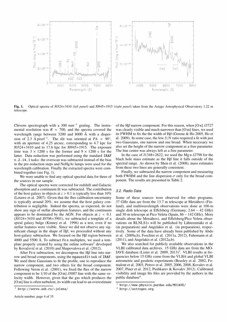
Fig. 1. Optical spectra of J0324+3410 (left panel) and J0945+1915 (right panel) taken from the Asiago Astrophysical Observatory 1.22 mtelescope.

Chivens spectrograph with a 300 mm−1 grating. The instru-mental resolution was R ≈ 700, and the spectra covered thewavelength range between 3200 and 8000 Å with a disper-sion of 2.3 Å pixel−1. The slit was oriented at PA = 90,with an aperture of 4.25 arcsec, corresponding to 4.7 kpc forJ0324+3410 and to 17.6 kpc for J0945+1915. The exposuretime was 3 × 1200 s for the former and 9 × 1200 s for thelatter. Data reduction was performed using the standard IRAFv.2.14.1 tasks: the overscan was subtracted instead of the biasin the pre-reduction steps and NeHgAr lamps were used for thewavelength calibration. Finally the extracted spectra were com-bined together (see Fig. 1).

We were unable to find any optical spectral data for three ofthe sources in our sample.

The optical spectra were corrected for redshift and Galacticabsorption and a continuum fit was subtracted. The contributionof the host galaxy in objects at z > 0.1 is typically less than 10%(Letawe et al. 2007). Given that the flux calibration uncertaintyis typically around 20%, we assume that the host galaxy con-tribution is negligible. Indeed the spectra, as expected, do notshow any sign of stellar absorption features, and the continuumappears to be dominated by the AGN. For objects at z < 0.1(J0324+3410 and J0706+3901), we subtracted a template of aspiral galaxy bulge (Kinney et al. 1996) as a test, even if nostellar features were visible. Since we did not observe any sig-nificant change in the shape of Hβ, we proceeded without anyhost-galaxy subtraction. We focused on the Hβ region between4000 and 5500 Å. To subtract Fe ii multiplets, we used a tem-plate properly created by using the online software2 developedby Kovacevic et al. (2010) and Shapovalova et al. (2012).

After Fe ii subtraction, we decompose the Hβ line into nar-row and broad components, using the ngaussfit task of IRAF.We used three Gaussians to fit the profile, one to reproduce thenarrow component, and two others for the broad component.Following Veron et al. (2001), we fixed the flux of the narrowcomponent to be 1/10 of the [O iii] λ5007 line with the same ve-locity width. However, given that the gas which produces the[O iii] line is often turbulent, its width can lead to an overestimate

2 http://servo.aob.rs/~jelena/

of the Hβ narrow component. For this reason, when [O ii] λ3727was clearly visible and much narrower than [O iii] lines, we usedits FWHM to fix the the width of Hβ (Greene & Ho 2005, Ho etal. 2009). In some case, the low S/N ratio required a fit with justtwo Gaussians, one narrow and one broad. When necessary wealso set the height of the narrow component as a free parameter.The line centre was always left as a free parameter.

In the case of J1348+2622, we used the Mg ii λ2798 for theblack hole mass estimate as the Hβ line it falls outside of thespectral range. As shown by Shen et al. (2008), mass estimatesfrom these two lines are generally consistent.

Finally, we subtracted the narrow component and measuringboth FWHM and the line dispersion σ only for the broad com-ponent. The results are presented in Table 2.

3.2. Radio Data

Some of these sources were observed for other programs.37 GHz data are from the 13.7 m telescope at Metsähovi (Fin-land), and multiwavelength observations were done at 100-msingle dish telescope at Effelsberg (Germany, 2.64 − 42 GHz)and 30-m telescope at Pico Veleta (Spain, 86 − 142 GHz). Moredetails about the Metsähovi, and Effelsberg/Pico Veleta obser-vations on RLNLS1s will be published by Lähteenmäki et al.(in preparation) and Angelakis et al. (in preparation), respec-tively. Some of the data have already been published by Abdoet al. (2009a,b), Foschini et al. (2011a, 2012), Fuhrmann et al.(2011), and Angelakis et al. (2012a,b).

We also searched for publicly available observations in theVLBI calibrated data archives. 15 GHz data are from the MO-JAVE database (Lister et al. 2009, 2013)3. VLBI results at fre-quencies below 15 GHz come from the VLBA and global VLBIastrometric and geodetic experiments (Beasley et al. 2002, Fo-malont et al. 2003, Petrov et al. 2005, 2006, 2008, Kovalev et al.2007, Piner et al. 2012, Pushkarev & Kovalev 2012). Calibratedvisibility and image fits files are provided by the authors in thepublic database4.

3 http://www.physics.purdue.edu/MOJAVE/4 http://astrogeo.org


http://servo.aob.rs/~jelena/

http://www.physics.purdue.edu/MOJAVE/

http://astrogeo.org


We performed a standard CLEANing (Högbom 1974) andfollowed the model-fitting of the calibrated VLBI visibility datain Difmap (Shepherd 1997). We preferred to use circular Gaus-sian components unless the use of elliptical components gave abetter fit to the data. To ensure the quality of the fit, we comparedGaussian model parameters with the results of CLEAN. The to-tal flux density and residual RMS appeared to be almost identicalfor the two cases. All of these sources have simple radio struc-ture, so they are well-modelled by Gaussian components. Theresults are presented in the Online Material (Table 7).

3.3. Online catalogues and Literature

We supplemented these data with information from online cat-alogues and literature. For γ rays, we mainly referred to Fos-chini (2011a), who reported the detection of 7 RLNLS1s withFermi/LAT after 30 months of operations. When available, wereported more recent published analyses (Foschini et al. 2012,D’Ammando et al. 2013a,d, Paliya et al. 2014). No new detec-tions have been claimed to date after Foschini (2011a). There-fore, for the non-detected sources in the present sample, weindicated the upper limit of ∼ 10−9 ph cm−2 s−1 as from theFermi/LAT performance web page5, which is the minimum de-tectable (TS = 25) flux above 100 MeV over a period of 4 yearsfor a source with a power-law shaped spectrum with a spectralindex α = 1. A summary of γ ray characteristics found in litera-ture is shown in the Online Material (Table 4).

For X-rays, we searched for missing sources in the Chan-dra X-Assist (CXA, Ptak & Griffiths 2003) catalogue v.4 andXMM–Newton Slew Survey Clean Sample v.1.5 (XSS, Saxton etal. 2008). The two catalogues provide X-ray detections in differ-ent energy bands: 0.5–8 keV for the former, and 0.2–12 keV forthe latter. The fluxes were then converted into the 0.3–10 keVband by using WebPIMMS6 and a fixed photon index value Γ = 2(α = 1). Some sources were not observed by any of the above-cited satellites. In those cases, we calculated an upper limit byusing the detection limit of the ROSAT All-Sky Survey (RASS,Voges et al. 1999, 2000).

At infrared/optical/ultraviolet wavelengths, in addition to theSwift/UVOT data presented here, we used SDSS-III data release9 (Ahan et al. 2012) and 2MASS (Cutri et al. 2003). Only onesource, J2021−2235, remained without optical coverage fromeither Swift/UVOT or SDSS, but we found B and R magnitudesin the US Naval Observatory B1 catalogue (Monet et al. 2003).

We also searched the WISE all-sky catalogue (Wright et al.2010) for photometric data at mid-IR wavelengths (between 3.4and 22 µm). In particular, we have used the last version of thecatalogue, the AllWISE data release (November 2013). All theRLNLS1s of the sample are detected (S/N > 3) in the WISEsurvey at 3.4 and 4.6 µm (W1 and W2 bands, respectively) while41 and 37 objects are detected also at 12 µm (W3 band) and22 µm (W4 band) respectively. The observed magnitudes havebeen converted into monochromatic flux densities assuming apower-law spectrum with α = 2. For the sources not detected ordetected with a S/N < 3, we have calculated the 3σ upper limiton the flux density.

At radio frequencies, in addition to the above cited programs(see Sect. 3.2), we have taken all available data from the NED7

and HEASARC8 archives.

5 http://www.slac.stanford.edu/exp/glast/groups/canda/lat_Performance.htm6 http://heasarc.gsfc.nasa.gov/Tools/w3pimms.html7 http://ned.ipac.caltech.edu/8 http://heasarc.gsfc.nasa.gov/

4. Observational characteristics

4.1. Gamma rays

We found in the available literature 7/42 detections at high-energy γ rays (17%) sources. Specifically, they are:

– J0948+0022, the first RL-NLS1 to be detected in γ rays(Abdo et al. 2009a,b, Foschini et al. 2010).

– J0324+3410, J1505+0326, and J2007−4434, which weredetected after the first year of Fermi operations (Abdo et al.2009c).

– J0849+5108, which was detected because of an outburst in2010 (Foschini 2011a, D’Ammando et al. 2012).

– J1102+2239, J1246+0238 (Foschini 2011a).

The spectral indices are generally steep, with a weighted av-erage of αγ = 1.6± 0.3 (median 1.7), but there is one interestingcase with harder spectrum: J0849+5108 with αγ = 1.0 − 1.18(Online Material Table 4 and 8). The average values for blazarsas measured by Fermi/LAT (Ackermann et al. 2011) are 1.4±0.2for FSRQs, α = 1.2 ± 0.1 for low-synchrotron peak BL Lacs,α = 1.1 ± 0.1 for intermediate-synchrotron peak BL Lacs, andα = 0.9±0.2 for high-synchrotron peak BL Lacs. Therefore, weconclude that the spectral characteristics of RLNLS1s are gener-ally similar to those of FSRQs.

Short timescale variability for factor-of-two flux changes isalso reported by some authors. Specifically, Foschini (2011a)reported intraday variability for J0948+0022 and J1505+0326,while Palyia et al. (2014) found 3-hour variability ofJ0324+3410 during its outburst of 2013 August 28 to 2013September 1 (see Online Material Table 9).

4.2. X-rays

About 90% of the sources in the present sample (38/42) are de-tected in X-rays (see Table 5). The average spectral index in the0.3–10 keV energy range is αX = 1.0± 0.5, with a median valueof 0.8 (see Online Material Table 8), as compared with the val-ues of 0.58 (FSRQs), 1.3 (BL Lac objects), 1.1 (BLS1s), and 1.7(RQNLS1s). These values were calculated from the samples ofγ−ray blazars from Ghisellini et al. (2009, 2010) and Tavecchioet al. (2010) and radio-quiet Seyferts from Grupe et al. (2010).The corresponding distributions are displayed in Fig. 2. The av-erage spectral indices for the individual sources (see Online Ma-terial Table 8) are α < 1 in 23/42 cases and α ≥ 1 in 12/42 cases.In 7/42 cases, the spectral index is near the boundary.

We note that the X-ray spectral indices of RLNLS1s aresimilar to those of BLS1s, and usually harder than those ofRQNLS1s. However, when compared to blazars, RLNLS1s arebetween the average values of FSRQs and BL Lac objects. Frominspection of the SEDs (see Sect. 7), it seems that the X-rayemission of RLNLS1s could be due either to inverse-Compton(IC) radiation from a relativistic jet or from the corona of the ac-cretion disk. This could explain why the average spectral indexis softer than that of FSRQs, where the X-ray emission is dom-inated by the IC from the jet (see, for example, Ghisellini et al.2010).

In the case of four sources, there were multiple observationswith sufficient exposure for individual detections (Online Ma-terial Table 5). We therefore searched for any correlation be-tween flux and spectral slope. No significant trend was found.It is interesting to compare with radio-quiet Seyferts, where acorrelation between 2–10 keV flux and the spectral index wasfound, indicating a steepening of the spectral shape as the flux


http://www.slac.stanford.edu/exp/glast/groups/canda/lat_Performance.htm

http://heasarc.gsfc.nasa.gov/Tools/w3pimms.html

http://ned.ipac.caltech.edu/

http://heasarc.gsfc.nasa.gov/

05

1015

Nr

RLNLS10

510

15

Nr

BL Lac Obj

05

1015

Nr

FSRQ

05

1015

Nr

BLS1

0 0.5 1 1.5 2 2.5 3

05

1015

Nr

Spectral Index (α)

NLS1

Fig. 2. X-ray (0.3–10 keV) spectral index distributions for the presentsample of RLNLS1s; BL Lac objects and FSRQs are from Ghisellini etal. (2009, 2010) and Tavecchio et al. (2010); BLS1s and RQNLS1s arefrom Grupe et al. (2010).

increases (Markowitz et al. 2003). Some interesting episodeswere described in the case of J0324+3410 by Foschini et al.(2009), Foschini (2013), and Tibolla et al. (2013): the sourcehas generally a soft spectral index, typical of NLS1s, but some-times — as the jet became active — the X-ray spectrum displaysa break at a 2–3 keV and a hard tail appears (see also Paliyaet al. 2014). Similar behaviour has been observed in anotherRLNLS1, PKS 0558−5049, where ASCA observed a hardeningof the spectral index during an outburst, changing from ∼ 1.2 to∼ 0.9 (Wang et al. 2001).

In the case of J0324+3410, with more data (Online MaterialTable 5), there is no evident trend to link the change in flux with achange of the spectral slope. Although the epochs with a hard tailare concentrated in a high-flux region, there are also observationswith similar fluxes that can be fit satisfactorily by a single power-law model. It is worth noting that there might be an instrumentalbias: Swift/XRT has a small effective area at energies ≥ 7 keV(Romano et al. 2005) and, therefore, the detection of the hard tailcould depend on the exposure time at similar flux levels. Indeed,the exposures in the present data set ranged from 1.3 to 8.8 ks(see Online Material Table 5) and the spectral shape at shorterexposures — having low statistics at high energies — could befit with just a power-law model with an index harder than usual.An observing campaign with a satellite like XMM–Newton forexample, carrying X-ray instruments with a large effective areaabove 7 keV, could effectively monitor the spectral changes (seebelow the example of J0948+0022).

Many sources of the present sample were included in previ-ous surveys by Komossa et al. (2006a) and Yuan et al. (2008).In these studies, the X-ray characteristics were measured fromROSAT data. Komossa et al. (2006a) found spectral indicesin the range 0.9–3.3, while Yuan et al. (2008) measured val-ues between 0.37 and 2.36. Particularly, the spectral index ofJ0948+0022 was measured as 1.6 ± 1.8 by Zhou et al. (2003),∼ 1.2 by Komossa et al. (2006a), and 1.26 ± 0.64 by Yuan etal. (2008). The source is also present in the Williams et al.(2002) sample, who reportedαX = 1.8±0.5, again on the basis ofROSAT observations. In our case, both Swift and XMM–Newton

9 This source is not in the present sample because it has a steep radiospectral index. It is included in the sample studied by Berton et al. (inpreparation).

indicate a harder spectral index (average αX ∼ 0.56) that re-mains unchanged with flux variations (Online Material Table 5).This is in agreement with previous studies and MW campaigns(Abdo et al. 2009a,b, Foschini et al. 2011a, 2012). A studybased on a long one-orbit XMM–Newton observation revealedthe presence of a soft X-ray excess (D’Ammando et al. 2014,Bhattacharyya et al. 2014), which is confirmed in the presentstudy. The break energy is between 1.72+0.09

−0.11 keV (D’Ammandoet al. 2014) and ∼ 1.2 keV (Bhattacharyya et al. 2014; see alsoour analysis in the Online Material Table 5). The low-energyspectral index is between 1.1 and 1.3, while the high-energypower-law has a slope 0.5–0.6. There is also a Swift observa-tion the same day of that of XMM–Newton (2011 May 28) andwe tried also to fit these data with a broken power-law model.We found α1 = Γ1 − 1 = 1.8+1.4

−0.8, α2 = Γ2 − 1 = 0.5 ± 0.2,and Ebreak = 0.9 ± 0.3 keV (χ2 = 5.4 for 7 dof, not reportedin Online Material Table 5). However, according to our thresh-old defined in Sect. 3, the broken power-law model is not sta-tistically preferred over the single power-law model (95% vs. athreshold of 99%). Therefore, we conclude that the presence orabsence of a soft X-ray excess is related more to an instrumen-tal bias rather than to an effective change of the AGN. ROSAT,having a bandpass of 0.1–2.4 keV, is biased toward soft X-raysources and therefore only captures the soft excess. Swift, witha wider energy band (0.3–10 keV) and snapshot observations,measured an average of both the soft excess and the hard tail.XMM–Newton, still operating in the 0.3–10 keV band, detectedboth the soft excess and the hard tail because of the longer ex-posure and larger effective area. Both D’Ammando et al. (2014)and Bhattacharyya et al. (2014) concluded that the excess at lowenergies could be due to the accretion disk/corona system, as isthe usual case for many RQNLS1s (e.g. Leighly 1999, Foschiniet al. 2004, Grupe et al. 2010).

We note that also the blazar 3C 273 displays such a soft ex-cess and there is a correlation between the low activity of the rel-ativistic jet and the emergence of the thermal component in thesoft X-rays, which was interpreted as a signature of the jet-diskconnection (Grandi & Palumbo 2004, Foschini et al. 2006). Inthe present case, the instrumental bias prevents any conclusionabout the X-ray component, but the optical component offerssome hints that support the above hypothesis (see Sect. 7).

The case of J2007−4434 is different. The X-ray spectrum asobserved by XMM–Newton on 2004 April 11 shows a soft ex-cess and a hard tail. Gallo et al. (2006) favoured the hypothesisof an accretion disk corona to generate the excess low-energyflux, while Foschini et al. (2009), on the basis of different vari-ability characteristics (16% and < 8% in the 0.2–1 keV and 2–10 keV energy bands, respectively), suggested a similarity withlow-energy peaked BL Lac objects (i.e. the low-energy com-ponent is the tail of the synchrotron emission). This seems tobe confirmed by the analysis and modelling of the SED (Abdoet al. 2009c, Paliya et al. 2013b; see also the Sect. 7). In thepresent work, we find two more XMM–Newton archival obser-vations performed in 2012 (May 1 and October 18): in bothcases, there was no low-energy excess and the spectra were fitwith a single power-law model with spectral index α ≈ 0.7. It isworth noting that the flux was about one third that of the 2004observation, when the soft excess was detected.

In all the other cases, ROSAT observations reported by Ko-mossa et al. (2006a) and Yuan et al. (2008) are generally con-firmed.

The search for variability on short timescales resulted inmany significant detections of intraday variability, with fluxchanges greater than 3σ (Online Material Table 9). There are



hour timescales for J0134−4258, J0324+3410, J0948+0022,J1629+4007, and J2007−4434. It is worth noting that the mea-surements reported in Table 9 (Online Material) were only madefrom Swift/XRT data. We also analysed XMM–Newton data andfind variability on minute timescales (down to ∼ 2 minutes withflux change at the 11σ level in the case of J0948+0022). How-ever, we note that all XMM–Newton observations are affected bysoft-proton flares: although we corrected for both the anomalousparticle and photon backgrounds, we noted that minute-scalevariability is detected near periods of the light curve that are ex-cised because of high particle background. In addition, there isno confirmation of such short timescale variations in the Swiftdata, but it is worth noting that Itoh et al. (2013) found similarvalues from optical observations. These findings therefore re-quire a much more careful dedicated analysis and confirmationwith other instruments less affected by grazing-incidence parti-cle background (i.e. from X-ray satellites in low-Earth orbit).

The hour timescales found are much shorter than thoseexpected in case of changing obscuration, which could be∼10 hours in the most extreme case of NGC 1365 (see the re-view by Bianchi et al. 2012). In addition, fits of X-ray spectrado not require iron lines or obscuration in addition to the Galac-tic column, as expected from radio-loud AGNs, in contrast toradio-quiet AGNs (e.g. Reeves et al. 1997). The exceptionseems to be J0324+341, where Abdo et al. (2009c) reportedan unresolved iron line at EFe = 6.5 ± 0.3 keV with equivalentwidth of 147 eV (see also Paliya et al. 2014). By integratingall the available Swift snapshots (with a total exposure time of2.1 × 105 s), we basically confirm the previous measurements:EFe = 6.5 ± 0.1 keV, equivalent width ∼ 91 eV, and ∆χ2 = 13.1for two additional parameters (EFe and normalisation; we fixedσFe to 0.1 keV). XMM–Newton observations of J0948+0022 andJ1348+2622 only show a hint of an excess above 5 keV.

4.3. Ultraviolet, optical, and infrared frequencies

Spectral indices for ultraviolet and infrared frequencies were cal-culated by means of the two-point spectral index formula

α12 = −log(S 1/S 2)log(ν1/ν2)

, (1)

where S 1 and S 2 are the observed flux densities at fre-quencies ν1 and ν2, respectively. In the ultraviolet, we usethe Swift/UVOT observations, where ν1 = 1.16 × 1015 Hz andν2 = 1.47 × 1015 Hz refer to the uvw1 (λ = 2591 Å) and uvw2(λ = 2033 Å) bands, respectively. For infrared frequencies, weadopt the extreme filters of WISE: ν1 = 1.36 × 1013 Hz andν2 = 8.82 × 1013 Hz, corresponding to W4 and W1 filters, re-spectively. When one of the two filters only has an upper limit,we referred to the closest other filter with a detection, either W2(ν = 2.50 × 1013 Hz) or W3 (6.5 × 1013 Hz). Optical spec-tral indices were measured by fitting the spectra over the range∼ 3000–8000 Å.

The average ultraviolet spectral index is αuv = 0.7 ± 1.4(median 0.7), and the values for the individual sources weremeasured from the integrated flux densities (Online Material Ta-ble 6). This spectral index can be compared with the values of0.79 (median 0.61) for BLS1, and 0.85 (median 0.65) for NLS1in the Grupe et al. (2010) sample, also based on Swift/UVOTobservations. Ganguly et al. (2007) observed 14 radio-quiet lowredshift (z < 0.8) quasars with Hubble Space Telescope (HST) inthe range 1570–3180 Å and measured an average index of 0.87.

Pian et al. (2005), also with HST over the range ∼ 1570–4780 Å,observed 16 blazars and found αuv ≈ 1.16. In a previous studyon a larger sample of 47 radio-loud AGNs observed in the range1200 − 3000 Å with International Ultraviolet Explorer (IUE),Pian & Treves (1993) found an average αuv ≈ 1, with strongemission line quasars having αuv ≈ 1.38, BL Lac objects withαuv ≈ 0.97, and radio-weak BL Lacs with αuv ≈ 0.66. Fora control sample of 37 objects from the Palomar–Green (PG)bright quasar survey, an average αuv ≈ 0.84 was found. At thelevel of average values, the present sample is in agreement withthe values for radio-weak blazars, PG quasars, and radio-quietSeyferts.

The average optical spectral index of the present sample ofRLNLS1s is αo = 1.0 ± 0.8 (median 0.8), in agreement withthe previous surveys of RQNLS1 (Constantin & Shields, 2003)and RLNLS1s (Komossa et al. 2006a, Yuan et al. 2008). Acomparison with the optical slopes measured by Whalen et al.(2006) reveals similar slopes (particularly, Fig. 4 in Whalen et al.2006), with some exceptions likely due to the source variability.For example, J1159+2838 changed from αo ≈ −0.19 to 0.04,and J1358+2658 switched from αo ≈ 0.45 to 0.97. Vanden Berket al. (2001) integrated the SDSS spectra of more than 2200quasars and found an average αo ≈ 0.44. They also note thatby using only the low-redshift sources, the optical spectral indexbecomes steeper (αo ≈ 0.65). Our average value (αo ≈ 1.0)seems to be in agreement with this trend.

The average infrared spectral index as measured from WISEis αIR = 1.3 ± 0.3 (median 1.3), as expected in the case ofsynchrotron emission from a relativistic jet (see Massaro et al.2011, D’Abrusco et al. 2012, Raiteri et al. 2014). Fig. 3shows the distribution of WISE colours of the present samplecompared with the blazar strip by Massaro et al. (2011) andthe X-ray selected Type 1 and 2 AGNs by Mateos et al. (2012,2013). While most of the RLNLS1s are in the blazar/AGNregion, there are also some cases in the starburst region (cf.Fig. 1 in Massaro et al. 2011), suggesting the presence ofintense star-formation activity (typical of NLS1s, Sani et al.2010). Caccianiga et al. (2014) studied a steep-spectrumRLNLS1 (SDSS J143244.91+301435.3, which is not includedin the present sample because of its steep radio spectrum), andfound significant star-forming activity. In that case, since the jetis likely to be viewed at a large angle, it does not overwhelm theemission from the nearby environment. The RLNLS1s of thepresent sample were instead selected by their flat radio spectra,to extract the beamed population, and are hence dominated bysynchrotron emission. However, one source (J1505+0326) in thestarburst region was detected in γ rays, and two γ-ray RLNLS1shave W2−W3 > 3 (in the addition to the one cited earlier, there isalso J0948+0022, still around the synchrotron line). Specifically,J0948+0022 and J1505+0326 were among the most γ−ray ac-tive RLNLS1s of the present sample, therefore this result couldbe counterintuitive (except for J0948+0022, which is still nearthe synchrotron line). The explanation is in the epochs of theWISE observations, performed between 2010 Jan 7 (MJD 55203)and Aug 6 (MJD 55414). Comparing with the γ-ray light curvesdisplayed in Foschini et al. (2012), it is seen that J0948+0022was almost undetected during the WISE observations. In the caseof J1505+0326, D’Ammando et al. (2013a) detected the sourceby integrating over three-month time bins, but the flux in the firsthalf of 2010 remained at low level of order 10−8 ph cm−2 s−1.Therefore, it is likely that these sources could have strong star-forming activity that is sometimes overwhelmed by synchrotronemission from the jet. We also note that another RLNLS1 of thepresent sample, J2021−2235, is classified as an ultraluminous


1.5 2 2.5 3 3.5 4 4.5

0.5

11.

5

W1−

W2

W2−W3

AGN Wedge

WGS FSRQ

WGS BL Lac

Fig. 3. WISE colours of the present sample of RLNLS1s (filled orangestars indicated the γ-ray detected RLNLS1s). Different characteristicregions are also plotted: the blazar WISE Gamma-ray Strip (WGS) forBL Lacs (dashed line) and FSRQs (dotted line), as defined by Massaroet al. (2012) and the AGN wedge (dot-dashed line) as defined by Ma-teos et al. (2012, 2013) for X-ray selected AGNs. The continuous linecorresponded to a power-law emission (S ν ∝ ν−α) with α ranging from∼ −0.5 to ∼ +2.5.

infrared galaxy (ULIRG) by Hwang et al. (2007), thus support-ing the presence of intense star-forming activity.

A search for the shortest timescale for a factor-of-two changein flux demonstrates intraday variability for 7/42 sources (seeTable 10). There is some bias in this case, because not allSwift/UVOT observations were performed using all six filters.Two sources were extensively observed with almost all the sixfilters (J0324+3410 and J0948+0022) and displayed intradayvariability at all wavelengths. This is in agreement of previ-ous findings of extreme intraday optical variability reported byLiu et al. (2010), Itoh et al. (2013), Maune et al. (2013), andPaliya et al. (2013a). In particular, Itoh et al. (2013) reportchanges on timescale of minutes in the optical polarised flux ofJ0948+0022 on 2012 December 20, with a peak degree of polar-isation of 36%.

Jiang et al. (2012) examined WISE data in a search forinfrared variability among the 23 RLNLS1 of the Yuan et al.(2008) sample. They found three cases, also in the presentsample: J0849+5108, J0948+0022, and J1505+0326. Thefirst two sources displayed intraday variability, while the lattershowed significant flux changes over ∼6 months. The remain-ing 20 RLNLS1s of the Yuan et al. (2008) sample did not showvariability, most likely because of the weakness of the sources.

A more detailed analysis of the characteristics of the opti-cal spectra (line, bumps, blue/red wings) will be presented else-where (Berton et al. in preparation).

4.4. Radio

About half of the sources (21/42) in the present sample wereonly detected at 1.4 GHz so it is not possible to determine a radiospectral index. In the remaining half of the cases, it was possi-ble to estimate a spectral index between two frequencies below8.4 GHz (between 1.4 and 5 GHz in 13/21 cases). About 28% ofthese sources (12/42) were detected at frequencies in the MHzrange (74–843 MHz, see Table 9). In 4/42 cases (J0324+3410,J0849+5108, J0948+0022, and J1505+0326), spectral indicesbetween 5–15 and 15–37 GHz are measured, because of the MW

campaign of Effelsberg, Metsähovi, and RATAN-600 (Abdo etal. 2009a,b, Foschini et al. 2011a, 2012, Fuhrmann et al. 2011,Angelakis et al. 2012a,b). In only two cases (J0324+3140 andJ0948+0022) are there detections up to 142 GHz at Pico Veleta.The results are summarised in Online Material Table 8. In 7/13cases, the spectral indices αr were inverted. Three of thesecases were of γ−ray detected RLNLS1s. Two of these cases,J0324+3410 and J0849+5108 (two γ−ray sources), the averagespectral index was inverted at higher frequencies. The weightedmean αr was equal to 0.1 ± 0.3 (median 0.3).

Comparison with blazar samples reveals similar spectral in-dices. Abdo et al. (2010b) performed a linear regression ofall the available data in the 1–100 GHz frequency range of 48blazars of the Fermi LAT Bright AGN Sample (LBAS) and findan average value of α1−100 GHz = 0.03± 0.23. They found no dif-ferences between FSRQs and BL Lac objects. It is worth notingthat the RLNLS1 J0948+0022 of the present sample is also inthe LBAS list, but it is classified there as a low-synchrotron peakFSRQ. Abdo et al. (2010) find a radio spectral index of −0.645.

Another useful comparison is with the jetted AGNs of theMOJAVE sample: Hovatta et al. (2014) analysed the radio dataof 191 AGNs (133 FSRQs, 33 BL Lac objects, 21 radio galax-ies, and 4 unknown-type AGNs and calculated the spectral indexbetween 8.1 and 15.4 GHz. Also in this case, there is virtuallyno difference between FSRQs and BL Lac objects, −0.22 and−0.19, respectively.

Tornikoski et al. (2000) studied 47 Southern hemispheresources, mostly FSRQs (38), plus 6 BL Lac objects and 3 radiogalaxies (see also Ghirlanda et al. 2010 for a sample of blazarsin the Southern hemisphere) over a frequency range spanning2.3 to 230 GHz. The spectral indices are almost flat below8.4 GHz, with some differences between BL Lacs and high-polarisation quasars on one hand, and low-polarisation quasarson the other: while the latter have a somewhat steeper spectralindex (α2.3−8.4 GHz ≈ 0.05), the former have an inverted index(α2.3−8.4 GHz ≈ −0.13). For all the sources, the spectral index be-comes steeper at higher frequencies (α90−230 GHz ≈ 0.79). Niep-pola et al. (2007) studied a large sample (398) of only BL Lacobjects in the Northern hemisphere and found average values ofα5−37 GHz ≈ −0.25 and α37−90 GHz ≈ 0.0.

Our values are in agreement with these results: we find arather flat or inverted spectrum extending from all the avail-able frequencies (Online Material Table 8), as already foundby Fuhrmann et al. (2011) and Angelakis et al. (2012a,b, inpreparation). However, we note that most of the radio obser-vations refer to the first γ−ray RLNLS1s detected, which wereimmediately monitored with MW campaigns, i.e. J0324+3410,J0849+5108, J0948+0022, and J1505+0326. All the othersources in the present sample have been poorly observed in theradio. There are, however, programs to increase the database onthese sources at radio frequencies. The Metsähovi group is per-forming a multi-epoch variability program at 22 and 37 GHz onmore than 150 radio-loud AGNs, including 38 RLNLS1s of thepresent sample (Lähteenmäki et al., in preparation). Richards etal. (2014) is performing a high-spatial resolution study on 15RLNLS1s of the present sample with the VLBA at 5, 8, 15, and24 GHz, including polarisation.

Analysis of archival VLBI radio maps provides some fur-ther information (see Sect. 3.2 and Online Material Table 7).Again, the earliest γ−ray detected RLNLS1s were the mostheavily observed: J0324+3410, J0849+5108, and J0948+0022.The source J0324+3410 (7 observations at 15 GHz) displayed asmall flare in 2011, with compactness — defined as the core tototal flux density ratio — of order 0.6, which increased during



the flare to > 0.75. Polarisation is almost stable during theseobservations, but during the flare there is a marginal change inthe position angle of the electric vector (EVPA) with respect tothe jet direction (from 87 to 77). Also J0849+5108 showedan increase in the compactness (from 0.75 to 0.9) with flux den-sity. Between 2013 January and July (MJD 56313 − 56481),there was a swing in the EVPA (from 168 to 24, with an al-most stable jet direction) that preceded a γ−ray outburst (Eggenet al. 2013), which happened also in J0948+0022 (Foschini etal. 2011a). The latter has been observed 17 times at 15 GHz,and many of these epochs were already studied by Foschini etal. (2011a). The present reanalysis basically confirms and ex-tends the previous studies. It is worth noting that this source isvery compact (0.975) as also indicated by previous comparisonwith single-dish observations (Abdo et al. 2009b, Foschini et al.2011a, 2012). An exceptional radio core outburst on 2013 May 5(MJD 56417), when J0948+0022 reached a core flux density of0.862 Jy. This followed a strong outburst at γ-rays that occurredon 2013 January 1 (MJD 56293), as reported by D’Ammandoet al. (2013c). During the same period there was also a swingof the EVPA, changing from ∼ 82 on 2012 November 11 to∼ 125 on 2013 May 5. Moreover, Itoh et al. (2013) reportedstrong variability in optical polarisation in the same epoch (seeSect. 4.3).

The only source for which there are multifrequency obser-vations is J1505+0326, from 2 to 43 GHz. A detailed analy-sis is reported b D’Ammando et al. (2013a). It is very com-pact (0.95–0.97 at 15 GHz during flares), at level comparable toJ0948+0022. A flux density excess (∼ 0.1 Jy) outside the corehas been measured at 22 GHz in 2002. The EVPA–jet directionangle is quite unstable, changing from ∼ 61 to −100. We ob-served significant flux density increases only in the VLBI coresof all the observed sources (Table 8), suggesting that the locationof the γ-ray emission should be very close to the central blackhole.

Morphological studies of RLNLS1s have been published byDoi et al. (2006, 2007, 2011, 2012), Gu & Chen (2010), Girolettiet al. (2011), and Orienti et al. (2012). The emerging charac-teristics are (a) compact radio morphology, although there arekiloparsec scale structures in some cases (Doi et al. 2012), (b)high-brightness temperature of the core feature, indicating non-thermal processes, (c) flat or inverted spectra (although the sam-ples included also steep spectrum radio sources, which are ex-cluded from the present work), and (d) possible links with com-pact steep spectrum (CSS) and gigahertz peaked spectrum (GPS)radio sources, as also suggested by Oshlack et al. (2001) andGallo et al. (2006) for J2007−4434, Komossa et al. (2006a),Yuan et al. (2008), and more recently by Caccianiga et al.(2014). Doi et al. (2012) found that the detection of extendedemission is lower than expected from broad-line Seyferts andthey suggest it could be due to the lower kinetic power of jetsin low-mass AGNs, rather than the young age of the source. In-terestingly, also the radio core of RQNLS1s and Seyferts dis-play non-thermal characteristics, suggesting some link with jets(Giroletti & Panessa 2009, Doi et al. 2013).

Angelakis et al. (in preparation) have studied the vari-ability of four RLNLS1s detected at γ rays (J0324+3410,J0849+5108, J0948+0022, J1505+0326) at different radio fre-quencies. Brightness temperature measurements indicate mini-mum Doppler factors from 1.3 for J0324+3410 to 4.2 in the caseof J1505+0326.

The search for short variability resulted in only one case ofvariability on timescales of days: we measure an upper limit of2.6 days for J0948+0022 at 37 GHz. In the other cases, we find

106 107 108 109 101010−

710

−6

10−

510

−4

10−

30.

010.

11

L disc

[LE

dd]

Mass [MO. ]

Fig. 4. Accretion disk luminosity [Eddington units] vs. mass ofthe central black hole [M⊙]. The orange stars are the RLNLS1s of thepresent sample (see Table 2) and filled orange stars indicate those de-tected at γ rays; the red circles are the FSRQs, and the blue squares arethe BL Lac objects (blue arrows indicates upper limits in the accretionluminosity) from Ghisellini et al. (2010). We noted some BL Lacs withstrong accretion disk, in the region occupied by FSRQs: these are theso-called intruders (Ghisellini et al. 2011, Giommi et al. 2012).

variations on timescales of about one month, but this is likelydue to the one-month sampling rate of Effelsberg observations.Metsähovi (37 GHz) observed at a more intense sampling rateduring some MW campaigns (e.g. Abdo et al. 2009b, Foschiniet al. 2011a, 2012). Nieppola et al. (2007) reported variabilityon timescales of hours for some BL Lac objects, for example,∼8 hours for S5 0716 + 71, ∼1 hour for AO 0235+164, and∼6 hours for OJ 287. In the case of RLNLS1s, clearly highersampling rate MW campaigns are required.

5. Estimates of masses and accretion luminosities

The masses of the central black holes are given by

M = f

RBLRσ2line

G

, (2)

where RBLR is the size of the broad-line region (BLR) measuredby reverberation or estimated from scaling relations, σline is theline dispersion (or second moment of the line profile), G is thegravitational constant, and f is a dimensionless scale factor oforder unity (Peterson et al. 2004). We used the line dispersion,because it is less affected by inclination, Eddington ratio, andline profile (Peterson et al. 2004, Collin et al. 2006). We esti-mate the BLR radius by using the relationship between the lumi-nosity of the Hβ line and the radius of the BLR (RBLR) from therelationship of Greene et al. (2010),

log[

RBLR

10 light days

]

= 0.85 + 0.53 log[

L(Hβ)1043 erg s−1

]

. (3)

Following Collin et al. (2006), we adopt f = 3.85.The size of the BLR gives also the luminosity of the accretion

disk (RBLR ∝ L1/2disk, e.g. Ghisellini & Tavecchio 2009; see also


Table 2. Mass and Accretion luminosity estimated from optical data. Columns: (1) Name of the source; (2) Line dispersion σline of the broadcomponent of Hβ [km s−1]; (3) FWHM of the broad component of Hβ [km s−1]; (4) Hβ luminosity [1042 erg s−1]; (5) Black hole mass [107 M⊙];(6) Disk luminosity [1044 erg s−1]; (7) Disk luminosity [Eddington units]; (8) method adopted: A, from Asiago spectra; L, spectra from literature;M, derived from optical magnitudes; N, spectra downloaded from NED; S, from SDSS spectra.

Source σline FWHM LHβ M Ldisk Ldisk/LEdd MethodJ0100 − 0200 982 920 − 4.0 25.2 0.49 MJ0134 − 4258 1632 1241 2.77 7.1 8.61 0.09 L (Grupe et al. 2000)J0324 + 3410 1791 1868 0.53 3.6 1.50 0.03 AJ0706 + 3901 1839 1402 0.16 2.0 0.43 0.02 NJ0713 + 3820 2041 1901 9.28 21.2 31.0 0.11 NJ0744 + 5149 2122 1989 − 26.5 49.2 0.14 MJ0804 + 3853 1588 1523 2.74 6.7 8.51 0.10 SJ0814 + 5609 2759 2777 6.10 31.0 19.9 0.05 SJ0849 + 5108 1330 2490 1.32 3.2 3.94 0.09 SJ0902 + 0443 1491 1781 2.02 5.0 6.17 0.09 SJ0937 + 3615 1343 2192 0.59 2.1 1.68 0.06 SJ0945 + 1915 1730 2818 2.52 7.6 7.80 0.08 AJ0948 + 0022 1548 1639 3.73 7.5 11.8 0.12 SJ0953 + 2836 2407 2749 3.14 16.6 9.84 0.05 SJ1031 + 4234 3153 1822 2.08 22.9 6.37 0.02 SJ1037 + 0036 985 1776 1.75 2.0 5.31 0.20 SJ1038 + 4227 1615 1917 2.62 6.8 8.12 0.09 SJ1047 + 4725 1474 2237 5.80 8.6 18.9 0.17 SJ1048 + 2222 1742 718 1.39 5.7 4.16 0.06 SJ1102 + 2239 1940 2181 3.56 11.5 11.2 0.08 SJ1110 + 3653 1230 2081 1.07 2.4 3.14 0.10 SJ1138 + 3653 1231 1542 1.29 2.7 3.85 0.11 SJ1146 + 3236 1737 1977 3.79 9.5 12.0 0.10 SJ1159 + 2838 1907 2728 0.052 1.2 0.13 0.01 NJ1227 + 3214 694 1567 0.51 0.52 1.42 0.21 SJ1238 + 3942 940 1229 1.16 1.5 3.42 0.18 SJ1246 + 0238 1667 1756 1.80 5.9 5.45 0.07 SJ1333 + 4141 1589 2942 1.73 5.3 5.25 0.08 SJ1346 + 3121 1074 1503 0.64 1.4 1.83 0.10 SJ1348 + 2622 2192 3361 4.09 5.3 13.0 0.19 S (based on Mg ii λ2798.)J1358 + 2658 1471 1805 3.20 6.3 10.1 0.12 SJ1421 + 2824 1589 1724 7.18 11.2 23.7 0.16 SJ1505 + 0326 1409 1337 0.41 1.9 1.12 0.05 SJ1548 + 3511 1557 2217 4.37 8.3 14.0 0.13 SJ1612 + 4219 777 1200 0.87 0.88 2.53 0.22 SJ1629 + 4007 1246 1410 2.00 3.5 6.10 0.13 SJ1633 + 4718 945 931 0.36 0.79 0.98 0.10 SJ1634 + 4809 1856 1763 1.95 7.7 5.94 0.06 SJ1644 + 2619 1129 1486 0.51 1.4 1.42 0.08 SJ1709 + 2348 2377 1256 0.95 2.4 2.79 0.09 SJ2007 − 4434 1869 2844 1.62 7.0 4.8 0.052 L (Drinkwater et al. 1997)J2021 − 2235 491 460 − 3.75 2.91 0.60 M

Bentz et al. 2013), which in turn has been normalised to theEddington value

LEdd = 1.3 × 1038

(

M

M⊙

)

[erg s−1]. (4)

By using L(Hβ) — instead of the continuum at 5100 Å (or an-other wavelength), which is more conventional and generallymore accurate — to estimate the size of the BLR and the ac-cretion disk luminosity, we avoid the problem of contaminationof the flux by either the jet or the host galaxy.

The results are displayed in Table 2. In three cases (3/42), nooptical spectra were found. Therefore, we estimated the line dis-persion from the value of FWHM found in literature by using theratio FWHM/σline = 1.07, which is the average over the known

values of the present sample (39/42). This value is consistentwith what expected from NLS1s (cf. Peterson 2011). From theavailable optical magnitudes near 5100 Å we estimated the diskluminosity and the size of the BLR and then used eq. (2) to esti-mate the mass. We note that these sources have Eddington ratiosslightly greater than the others of the sample: this can be under-stood because with the photometry it is not possible to disentan-gle the contribution of the disk from that of the jet. We note thatour values are in agreement with the results available in the vastmajority of literature on RLNLS1s (e.g. Komossa et al. 2006,Whalen et al. 2006, Yuan et al. 2006) and on NLS1s in general(e.g. Peterson 2011).

A comparison of these data with the corresponding data forthe blazar sample is shown in Fig. 4. It is evident that RLNLS1s



occupy a unique parameter space among AGNs with relativis-tic jets that corresponds to lower masses and high Eddingtonrates10. There is apparently an unoccupied area of parameterspace corresponding to low black hole masses and low Edding-ton ratios. It is not possible to say whether this is real or a se-lection effect. Possible candidates to occupy this region are low-luminosity AGNs (e.g. M81, Alberdi et al. 2013), although thereis debate about the nature of their radio emission (see Paragi etal. 2013). Moreover, no low-luminosity AGN has yet been de-tected in high-energy γ rays.

6. Monochromatic luminosities

Another comparison with blazars can be done via νLν−νLν plotsin Fig. 5. Starting from the available data, we normalised thefluxes to four reference frequencies or wavelengths or energies:15 GHz for radio observations, 203 nm for ultraviolet wave-lengths, 1 keV for X-rays, and 100 MeV for γ−rays. While formost blazars, radio observations at 15 GHz were available fromthe MOJAVE project, the same was not true for RLNLS1s. Forhalf of the RLNLS1s (21/42), there were radio data at 1.4 GHzeither from NVSS or FIRST surveys. In some cases, there werealso data at 5, 8.4, 17, or 20 GHz (the two latter frequencies areused in the Southern hemisphere). We extrapolated the 15 GHzflux by using the average radio spectral indices in Online Mate-rial Table 8.

The situation is slightly better at ultraviolet wavelengths, be-cause of the availability of Swift/UVOT observations, many ofthem specifically requested for this survey. For those sourceswith incomplete data, we used the bluest photometric data avail-able and corrected by using the average UV spectral index inOnline Material Table 8. We adopted the average spectral in-dices also to normalise the integrated fluxes or upper limits inthe 0.3–10 keV and 0.1–100 GeV bands.

The monochromatic fluxes were then K-corrected by

S ν,rest = S ν(1 + z)αν−1, (5)

where S ν,rest is the rest-frame monochromatic flux at the fre-quency ν, S ν is the observed monochromatic flux at frequencyν, z is the redshift, and αν is the spectral index at the frequencyν. The corrected monochromatic fluxes were then converted intoluminosities. The results are displayed in Fig. 5.

Fig. 5 shows that RLNLS1s are the low-luminosity tail ofFSRQs, as already noted by Foschini et al. (2013). While at ra-dio and ultraviolet frequencies RLNLS1s share the same regionof BL Lac objects, the two populations diverge from each otherat 1 keV, where BL Lac objects move to greater X-ray luminosi-ties, indicating a different origin of the emission (synchrotron forBL Lacs, disk corona or inverse-Compton for RLNLS1s).

10 This part of text has been changed after November 4, 2019. Thefollowing sentence has been removed: “It is worth noting one outlier,J2007−4434, has a low Eddington rate (0.003LEdd): this was also oneof the RLNLS1s whose nature is questionable on account of its weakFe ii emission (Gallo et al. 2006, Komossa et al. 2006)”. In the previousversions, we referred to Oshlack et al. (2001) for the optical spectrumof J2007 − 4434. However, when following up the 2019 October γ−rayoutburst of this source (Berton et al. 2019), we found an error in the y-axis of the optical spectrum displayed in Fig. 2 of Oshlack et al. (2001).The same spectrum was originally recorded by Drinkwater et al. (1997),but the original 1997 figure has a flux greater than that of Oshlack bya factor ∼ 200. After adopting the correct flux value, J2007 − 4434 isnow fully consistent with the typical values of the NLS1s distributions.This change of flux affects Table 2, Fig. 4, and Fig. 13, left panel.

10−4 10−3 0.01 0.1 1 10 1000.01

0.1

110

100

1000

104

Gam

ma

rays

100

MeV

− ν

L ν [1

044 e

rg s

−1 ]

Radio 15 GHz − νLν [1044 erg s−1]

0.01 0.1 1 10 100 10000.01

0.1

110

100

1000

104

Gam

ma

rays

100

MeV

− ν

L ν [1

044 e

rg s

−1 ]

UV 203 nm − νLν [1044 erg s−1]

10−4 10−3 0.01 0.1 1 10 100 10000.01

0.1

110

100

1000

104

Gam

ma

rays

100

MeV

− ν

L ν [1

044 e

rg s

−1 ]

X−rays 1 keV − νLν [1044 erg s−1]

Fig. 5. Gamma-ray luminosity at 100 MeV compared with radioluminosity at 15 GHz (top panel), ultraviolet luminosity at 203 nm (midpanel), X-ray luminosity at 1 keV (bottom panel). The orange starsare the RLNLS1s of the present sample detected in γ rays, while upperlimits are reported for the others (grey arrows); the red circles are theFSRQs and the blue squares are the BL Lac objects.

We noted one possible outlier in the radio–γ panel:J1102+2239 was detected at γ-ray flux above what is expectedfrom the trend of the other sources. There could be several ex-planations: the γ-ray activity could be limited to a small timeinterval, the radio measurements, extrapolated from 1.4 GHzmeasurements from FIRST and NVSS, were likely done duringperiods of low activity of the sources, or it could even be an in-


1013 1014 1015 1016

10−

1210

−11

νFν

[erg

cm

−2

s−1 ]

Frequency [Hz]1013 1014 1015 1016

10−

1210

−11

νFν

[erg

cm

−2

s−1 ]

Frequency [Hz]

Fig. 6. Zoom of the SED of J0948+0022 in the infrared-to-ultraviolet range. Data are from: WISE (filled squares), 2MASS (filled triangles),SDSS (continuous line), Swift/UVOT (filled circles). (left panel) Blue refer to lowest observed activity state (LS, 2009 May 15); (right panel) redto highest activity state (HS, 2012 December 30). The grey dot-dashed line represents a model of standard accretion disk as expected in the case ofJ0948+0022 (M = 7.5 × 107 M⊙); the grey dotted line represents the synchrotron emission; the continuous grey line is the sum of the two models.

dication of some artefact in the γ-ray detection. Further studiescould solve the conundrum.

There are also two sources with very low X-ray fluxes in theX-ray/γ-ray panel, J0100−0200 and J0706+3901. In both cases,the X-ray flux was measured by Chandra in 2003 and there wereno simultaneous data at other wavelengths.

We stress the difference between RLNLS1s and BL Lac ob-jects. Fig. 5 shows the observed luminosities at different fre-quencies: RLNLS1s and BL Lacs occupy similar regions andgenerally overlap at radio and UV frequencies. However, whileBL Lac objects have low power and masses comparable to thoseof FSRQs, RLNLS1s have low power and lower masses (seeFig. 4). Indeed, when normalised for the mass of the centralblack hole, the jet power of RLNLS1s and FSRQs are of thesame order of magnitude, as shown by Foschini (2014) and ref-erences therein. It is worth stressing that the normalisation isnot linear, but it is necessary to divide the jet power by M1.4, ac-cording to the theory developed by Heinz & Sunyaev (2003) andconfirmed by Foschini (2011b, 2012b,c, 2014).

7. Spectral energy distribution

Fig. 8-13 display the observed SEDs of all RLNLS1 in thepresent sample, assembled from data extracted from observa-tions at different epochs and archives, as discussed in Sect. 3.The most complete SEDs are mostly those of the RLNLS1ssignificantly detected at gamma rays, i.e. J0324+3410,J0849+5108, J0948+0022, J1505+0326, J2007−4434. Themodelling of these SEDs already has been presented and dis-cussed in other papers (e.g. Abdo et al. 2009b,c, Foschini etal. 2011a, 2012, D’Ammando et al. 2012, 2013a,b, Paliya et al.2014).

There are also a few more cases (e.g,. J0814+5609,J1047+4725, J1548+3511, J1629+4007) with fairly good sam-pling because of previous specific interest. For example,J1629+4007 was long observed because it was thought to bean example of a high-frequency peaked FSRQ (Padovani et al.2002, Falcone et al. 2004). It is evident from the SED (Fig. 15)that the strong X-ray emission is not due to synchrotron radia-tion, but rather to the disk corona (see also Maraschi et al. 2008).In other cases, it seems simply that the source fell into the field

of view of other targets. We noted a strong change in radio fluxdensity at 5 GHz in J1047+4725: early observations performedin 1987 with the Green Bank 91 m telescope (∼ 3.′5 angular res-olution) found a flux density of ∼ 0.4 Jy (Becker et al. 1991,Gregory & Condon 1991), while an observation with the VLAat 8.4 GHz in 1990 (0′′.2 angular resolution) measured a flux den-sity of ∼ 0.3 Jy (Patnaik et al. 1992). A VLBA observation at5 GHz with milliarcsecond resolution in 2006 resulted in a fluxdensity of ∼ 33 mJy (Helmboldt et al. 2007). One explanationfor this could be the presence of significant extended emission,which is integrated in the low angular resolution of Green Bank91 m and VLA telescopes, while is resolved in the milliarcsec-ond images of VLBA.

Other sources displayed extreme variability, specifically atoptical wavelengths: for example, the SDSS optical spectrumof J0849+5108 (observed in 2000) is about one order of mag-nitude lower than the optical observations made with Swift afterthe detection at γ-rays by Fermi (2011–2013). A similar case isJ1159+2838, while the optical spectrum of J0953+2836 is abouttwo orders of magnitude brighter than in the Swift observations.Spectral changes at optical frequencies, due to the jet activity,are also observed. Just as an example, we focus on the infrared-to-ultraviolet band of J0948 + 0022, which is the best sampledsource, being the first to be detected at γ-rays. Fig. 6 displaysthe two extreme states from the available data: the lowest activ-ity state (LS, 2009 May 15, see also Abdo et al. 2009b, Foschiniet al. 2012) and the highest state (HS, 2012 December 30). Inboth cases, we model the synchrotron emission (dotted grey line)with a power-law model with an exponential cutoff. The diskemission (dashed grey line) is the standard Shakura–Sunyaevmodel as expected from a black hole of M = 7.5 × 107M⊙(see Table 2). Previous modelling (Abdo et al. 2009b, Fos-chini et al. 2012) supposed constant disk luminosity equal toLdisk ∼ 0.4LEdd, as measured by fitting the optical/UV emissionwith a standard Shakura–Sunyaev disk. In the present work, weobtained from the emission lines a value of Ldisk ∼ 0.12LEdd.The difference could be due to a contamination of the jet emis-sion in the optical/UV photometry fit, which is removed by usingthe emission lines. However, since the optical spectrum of SDSSwas observed in 2000 and the MW campaign used for the SED



modelling were obtained in 2008–2011, it is also possible thatthe Eddington ratio really changed.

Although the lowest flux points were not simultaneous, sincemany of them are smoothly connected, it is reasonable to assumethat they refer to a common state of low jet activity. Therefore,we modelled them together as low activity state (LS): in thiscase, the expected peak of the emission from the accretion diskat 12% of the Eddington luminosity is at ∼ 3.0×1015 Hz. For thehigh state (HS), we have just one Swift/UVOT observation andwe adopted a standard disk at 40% of the Eddington value, peak-ing at ∼ 4.1 × 1015 Hz. The cutoff of the synchrotron emissionwas set to 8 × 1014 Hz in the LS and increased to 1.5 × 1015 Hzin the HS. We underscore that this is just another option, in addi-tion — and not in contrast — to the previous model. As the ex-pected peak of the disk emission in the far UV, outside the rangeof our observations, we cannot clearly distinguish between dif-ferent possibilities. We also note that at infrared wavelengths,there is an excess that is likely attributable to the dusty torusand/or the host galaxy, as suggested also by the WISE colours(see Sect. 4.3).

Changes in the activity of a relativistic jet, as forJ0948+0022, could explain the differences in the spectral slopesof J0849+5108, and J1159+2838. All these sources havean optical spectrum with a slope different from that derivedfrom the optical/UV photometry. Moreover, some sourcesshow optical/UV slopes decreasing with increasing frequencies(e.g. J0804+3853, J0937+3615, J1031+4234, J1038+4227,J1102+2239, J1138+365, J1227+3214), while there were othercases with the opposite trend (e.g. J0134−4258, J0324+3410,J0814+5609, J1348+2622, J1548+3511, J1629+400). Thesealso have a flat X-ray slope, with some evidence of a soft-excess.An inspection of their corresponding central black hole massesand Eddington ratios did not reveal any trend. On the basis of theJ0948+0022 behaviour, we favour the interpretation of the samecentral engine observed in a different combination of jet–diskstates.

There are some cases with only a few data points, so that it isnot possible to draw useful inferences (e.g. J0100−0200,J0706+3901, J1333+4141, J1346+3121, J1358+2658,J1612+4219, J1709+2348). While we have added signif-icantly to the multiwavelength database for many of theseobjects, the radio observations remained limited to only1.4 GHz. It is therefore desirable that future observations focuson radio frequencies (e.g. Richards et al. 2014, Lähteenmäki etal., in preparation).

8. Jet power

To estimate the jet power, we adopted the relationships based onthe radio core measurements at 15 GHz by Foschini (2014),

log Pjet,radiative = (12 ± 2) + (0.75 ± 0.04) log Lradio,core (6)

and

log Pjet,kinetic = (6 ± 2) + (0.90 ± 0.04) log Lradio,core. (7)

From the values calculated in the Sect. 6, we derived the radia-tive, kinetic (protons, electrons, magnetic field), and the total jetpower for each source. The results are given in Table 3.

In some cases, it is possible to test the present results withcalculations performed by modelling the SED, with the caveatthat we are comparing different epochs of strongly variablesources. For example, J0948+0022 — the first RLNLS1 tobe detected at gamma rays — had a radiative jet power of

log Pradiative = 45.5, while the kinetic part was estimated aslog Pkinetic = 46.9 (Abdo et al. 2009a). During the 2009 MWcampaign, these values ranged from 44.9 to 45.54 for the radia-tive power, and from 45.67 to 46.2 for the kinetic power (Abdoet al. 2009b). During more than three years of monitoring,log Prad spanned the interval 44.55–45.97, while log Pkinetic wasin the range 46.19–47.61 (Foschini et al. 2012). The presentestimate (Table 3) is an average of several measurements donedirectly at 15 GHz (mostly by the MOJAVE project and Ef-felsberg), and is reasonably consistent with the previously pub-lished values (see also Angelakis et al., in preparation). Thegreater values were recorded during the exceptional 2010 out-burst, when J0948+0022 reached an observed luminosity ofabout 1048 erg s−1 (Foschini et al. 2011a).

In other cases:

– J0324+3410: log Prad = 42.8, log Pkin = 44.3 (averaged overone year, Abdo et al. 2009c), and log Prad = 41.29–41.74,log Pkin = 44.06–45.14 (different states over five years mon-itoring, Paliya et al. 2014).

– J0849+5108: log Prad = 45.6 (peak during an outburst),log Pkin = 45.3(11) (D’Ammando et al. 2012).

– J1505+0326: log Prad = 44.0, log Pkin = 46.2 (averaged overone year, Abdo et al. 2009c).

– J2007−4434: log Prad = 42.9, log Pkin = 44.1 (averaged overone year, Abdo et al. 2009c).

A comparison with the jet power of FSRQs and BL Lac ob-jects (Fig. 7) shows that RLNLS1s have values comparable toBL Lac objects but lower than FSRQs. The mean values arelog Prad = 43.35 and log Pkin = 43.62 for RLNLS1s, log Prad =

45.49 and log Pkin = 46.78 for FSRQs, and log Prad = 44.14and log Pkin = 45.01 in the case of BL Lac objects. Taking intoaccount a mean value for the masses of the central black holesof the three populations (MRLNLS1 = 6.8 × 107M⊙, MFSRQs =

1.5 × 109M⊙, and MBL Lacs = 7.2 × 108M⊙) and renormalizingby M1.4, we obtained log Prad = 32.38 and log Pkin = 32.65 forRLNLS1s, log Prad = 32.64 and log Pkin = 33.93 for FSRQs,and log Prad = 31.74 and log Pkin = 32.61 in the case of BL Lacobjects. Thus, the normalised jet power is almost the same for allthe three types of AGNs, as expected (see Sect. 6), and it is alsoconsistent with the jets from Galactic binaries (Foschini 2014).

9. Discussion

Since the discovery of NLS1s, there has been debate as towhether they are an intrinsically separate AGN class, or simplythe low-mass tail of the distribution of Seyferts (Osterbrock &Pogge 1985). Many authors favoured the latter hypothesis (e.g.Grupe 2000, Mathur 2000, Botte et al. 2004). The same questionhas been proposed in the case of RLNLS1s (Yuan et al. 2008).The first studies following the detections at γ rays suggested asimple mass difference (Abdo et al. 2009a,c, Foschini 2011a,2012a, Foschini et al. 2011a, 2013). The unification of rela-tivistic jets provided further support for this point of this view(Foschini 2011b, 2012b,c, 2014). On the basis of what we havefound in this survey, with more sources and data, we can confirmthat, although RLNLS1s show some peculiar observational dif-ferences with respect to the other radio-loud AGNs (the opticalspectrum and the possible starburst activity), the physical char-acteristics inferred from the data (mass of the central black hole,Eddington ratio, spectrum, jet power) favour the hypothesis thatRLNLS1s are the low-mass tail of AGNs with jets. This is one

11 Electrons and magnetic field only.


010

2030

Nr

RLNLS1

010

2030

Nr

FSRQ

40 42 44 46 48 50

010

2030

Nr

Radiative Jet Power [log erg s−1]

BL Lac Obj

010

2030

Nr

RLNLS1

010

2030

Nr

FSRQ

40 42 44 46 48 50

010

2030

Nr

Kinetic Jet Power [log erg s−1]

BL Lac Obj

Fig. 7. Jet power distribution: (left panel) radiative, (right panel) kinetic. RLNLS1sdata are from the present work (Table 3), while values forFSRQs and BL Lac objects are from Ghisellini et al. (2010).

more point favouring the Livio (1997) conjecture, according towhich the jet engine is the same, but the observational featuresare different, depending on a number of variables, such as themass of the central accreting body, the accretion flow, and thelocal environment.

In the case of RLNLS1s, the relatively lower mass of thecentral black hole implies variability on very short timescales,much smaller than expected only from Doppler boosting, whichis exactly what is seen when the observational coverage allowsit. It is known that the power spectral densities of AGNs showa break timescale, tb, separating long-term timescales from theshorter ones (McHardy et al. 2006). There are some relation-ships linking tb with the mass of the central black hole, thebolometric luminosity, or the FWHM of the Hβ (McHardy etal. 2006, González-Martín & Vaughan 2012). By taking as rep-resentative values the averages of the selected quantities, it ispossible to estimate tb, which is expected to be around minutesto hours for RLNLS1s, and hours to a few days for blazars. In-deed, hour timescales at high energies are exceptional events forblazars (e.g. Foschini et al. 2011b,c), but are quite common forRLNLS1s as there are sufficient statistics to allow a meaningfuldetection (Table 10). As stated in Sect. 4.2, the claim of minutetimescale X-ray variability requires further detailed study, but itis worth noting the 2–3 minute timescale variability in the opticalpolarisation reported by Itoh et al. (2013).

We have observed not only flux variability, but also spec-tral changes, suggesting the interplay of jet and disk compo-nents (see the case of J0948+0022 in Sect. 7). At a first look,the SEDs suggest two different classes of RLNLS1s, depend-ing on the slope of the optical/UV spectra. However, the spec-tral variability of some sources (e.g. J0849+5108, J0945+1915,J0948+0022, J1159+2838) simply indicates that we are observ-ing different states of activity of the same central engine. Indeed,the two classes do not show any difference in the mass, disk, andjet parameters.

The lower mass of the central black holes in RLNLS1s has animportant implication: the observed jet luminosity is lower thanthat of quasars, but comparable to that of BL Lac objects. There-fore, one could wonder why the RLNLS1s are more difficult todiscover than BL Lacs? The latter are generally more luminousat X-rays than RLNL1s because the synchrotron radiation peaksin the UV/X-rays (see Fig. 5, bottom panel), and indeed, BLLac objects are more easily found in X-ray surveys (Padovani &

Giommi 1995). At γ rays, Fermi/LAT discovered many BL Lacobjects because the instrumental characteristics of LAT favourhard sources at low fluxes: this made it easier to detect BL Lacs(αγ < 1), but not RLNLS1s (αγ > 1) (see Sect. 4.1). At radiofrequencies, both RLNLS1s and BL Lac objects are weak (seeFig. 5, top panel). However, Giroletti et al. (2012) noted thatBL Lacs have extended radio emission, which is almost missingin RLNLS1s (e.g,. Doi et al. 2012). One possible explanation,advanced by Doi et al. (2012), is that in the case of RLNLS1s,the jet has low kinetic power because of the low mass and be-cause it has to propagate in a gas-rich environment, while in BLLacs the jet power is slightly greater and develops in a more rar-ified medium. Another possibility is to invoke the young age ofRLNLS1s (Mathur 2000, Mathur et al. 2012) and, indeed, manyauthors made the hypothesis of a link with GPS/CSS sources,which in turn are believed to be very young radio galaxies (Osh-lack et al. 2001, Komossa et al. 2006a, Gallo et al. 2006, Yuanet al. 2008, Caccianiga et al. 2014). Yet another option hasbeen proposed by Gu & Chen (2010): the jet activity could beintermittent, as observed in other Seyferts (e.g. Brunthaler etal. 2005, Mundell et al. 2009). Therefore, as the technolog-ical improvement of radio surveys allows better monitoring ofthese sources (e.g. Square Kilometer Array, SKA), the rate ofdetection should increase.

The intermittent jet should not be confused with the out-burst/flare activity as observed in blazars. In the case ofRLNLS1s, the periods of activity/inactivity might be separatedby dramatic changes in flux. Indeed, in addition to the episodesof strong variability already described (see Sect. 7), we also notetwo sources where the X-ray flux was three-to-four orders ofmagnitude lower than the optical/UV emission (J0100−0200,J0706+3901). In other cases, although the SED displayed thedouble-humped shape typical of a domination of a relativis-tic jet, the lack of γ-ray detection (no new detection was re-ported to date) set very stringent constraints (e.g. J0814+5609,J1031+4234, J1421+2824, J1629+4007). This can be comparedwith the lowest-known state of the BL Lac object PKS 2155−304(z = 0.116) where the changes in the X-ray flux were of about anorder of magnitude and there was a shift of the synchrotron peakat lower frequencies (Foschini et al. 2008). This indicates a jetwith a continuous background of emitted radiation, with super-imposed outbursts and flares, as new blobs are ejected. The moredramatic changes of three-to-four orders of magnitudes observed



Table 3. Estimated jet power from radio core measurements at 15 GHz according to the relationships in Foschini (2014). Columns display thelogarithm of the radiative, kinetic (protons, electrons, magnetic field), and total jet powers [erg s−1].

Source log Prad log Pkin log Ptot

J0100 − 0200 42.88 43.06 43.28J0134 − 4258 43.28 43.53 43.72J0324 + 3410 43.17 43.40 43.60J0706 + 3901 42.22 42.27 42.55J0713 + 3820 42.67 42.81 43.05J0744 + 5149 43.55 43.86 44.03J0804 + 3853 42.59 42.71 42.96J0814 + 5609 43.88 44.26 44.41J0849 + 5108 44.58 45.09 45.21J0902 + 0443 44.33 44.79 44.92J0937 + 3615 42.56 42.67 42.92J0945 + 1915 43.37 43.64 43.83J0948 + 0022 44.72 45.27 45.38J0953 + 2836 44.25 44.70 44.83J1031 + 4234 43.54 43.85 44.02J1037 + 0036 44.00 44.40 44.55J1038 + 4227 42.57 42.68 42.93J1047 + 4725 44.92 45.50 45.60J1048 + 2222 42.59 42.71 42.95J1102 + 2239 42.98 43.18 43.40J1110 + 3653 43.92 44.31 44.46J1138 + 3653 43.41 43.70 43.88J1146 + 3236 43.64 43.97 44.14J1159 + 2838 42.51 42.61 42.86J1227 + 3214 42.58 42.70 42.95J1238 + 3942 43.72 44.06 44.22J1246 + 0238 43.34 43.61 43.79J1333 + 4141 42.51 42.61 42.87J1346 + 3121 42.42 42.50 42.76J1348 + 2622 43.38 43.65 43.84J1358 + 2658 42.76 42.91 43.14J1421 + 2824 43.77 44.12 44.28J1505 + 0326 44.57 45.08 45.20J1548 + 3511 44.10 44.52 44.66J1612 + 4219 42.74 42.88 43.12J1629 + 4007 43.73 44.07 44.24J1633 + 4718 42.76 42.91 43.14J1634 + 4809 43.46 43.75 43.93J1644 + 2619 43.31 43.57 43.76J1709 + 2348 42.42 42.58 42.81J2007 − 4434 43.96 44.36 44.50J2021 − 2235 42.99 43.19 43.40

in RLNLS1s suggests that the central engine changes its level ofactivity significantly: not only the jet, but also the corona seemsto be strongly reduced.

Czerny et al. (2009), supported by Wu (2009), proposed a ra-diative instability in the accretion disk to explain the intermittentactivity in young radio sources. RLNLS1s have all accretion lu-minosities sufficiently high to be in the radiation-pressure dom-inated regime (Moderski & Sikora 1996, Ghosh & Abramow-icz 1997; see Foschini 2011b for the application to RLNLS1s),where Czerny’s theory applies. The timescale of the active phasein the case of low-mass AGNs, such as NLS1s, could be verysmall, of the order of tens-to-hundreds of years (Czerny et al.2009). Therefore, the low kinetic power of the jet due to thelow mass of the central black hole, the short periods of activ-ity, and a frustrating nearby environment rich in interstellar gasand photons, are the sufficient ingredients to explain the lack of

extended radio relics. As suggested by Doi et al. (2012), suchstructures might appear only in the sources with greatest blackhole masses, which in turn might be in the final stages of theircosmological evolution before changing into broad-line AGNs.

Another possibility is the aborted jet model proposed byGhisellini et al. (2004), which in turn could also explain the dif-ference between radio-loud and radio-quiet AGNs. In this case,the jet has insufficient power to escape from the central blackhole and falls back. The spectral characteristics in the X-rayband could be an index generally steeper than usual for Seyferts(that is αx ∼ 1), significant equivalent-width fluorescent ironlines, and a steeper-when-brighter behaviour of the light curves.J0324+3410 might be a good candidate, also because it is theonly one with a detected Fe Kα line. However, the X-ray fluxand spectral index values (Online Material Table 5) do not re-veal any significant trend. We note that high-flux periods have


both harder and steeper indices. We can speculate that a jetmight sometimes be aborted (steeper when brighter) or launched(harder when brighter). The rather obvious question is then whatdetermines one or the other?

10. Conclusions

We have presented a survey of 42 RLNLS1s observed from radioto γ rays, the largest MW sample to date of this type of source.In addition to previously published data, we present here newanalyses of data obtained with Swift and XMM–Newton specifi-cally to address these sources. The main results of the analysesare:

– γ rays: 7/42 sources (17%) were detected at high-energy γrays. The average spectral index is αγ ∼ 1.6, consistent withthat of FSRQs. Intraday variability has been reported in threesources.

– X-rays: We detected 38/42 sources (90%), with an averagespectral index αx ∼ 1.0 and median 0.8. We also detectedvariability on timescales of hours in 6 sources.

– Intraday variability was observed also at ultraviolet/opticalwavelengths in those few sources which were targets ofMW campaigns. Dramatic changes both in fluxes and spec-tra were also observed when comparing observations ontimescales of years. Infrared colours indicate that RLNLS1sare basically on the line expected from synchrotron emission,but with a significant spread towards the starburst region.

– We observed in some sources changes of the EVPA corre-sponding to γ ray activity. We detected significant changesof radio flux density only in the VLBI-cores, suggesting thatthe emission of γ rays should occur close to the central blackhole.

– Comparison of monochromatic luminosities at 15 GHz,203 nm, 1 keV, and 100 MeV with a sample of blazars (FS-RQs, and BL Lac objects) suggest that RLNLS1s are thelow-power tail of the quasar distribution.

– Some SEDs confirm the dramatic variability already appar-ent from the single band analysis. We modelled one case(J0948+0022) to show how the observed spectral variabilitycan be interpreted as the interplay of the jet and accretiondisk emission.

The radio coverage are still deficient, but some programs areongoing (Richards et al. 2014, Angelakis et al. in preparation,Lähteenmäki et al. in preparation).

The main results calculated from the data are:

– The estimated masses of the central black holes (106−8M⊙)and Eddington ratios (0.01–0.49LEdd) are in the range typi-cal of NLS1s. The masses are lower than those of blazars(108−10M⊙), indicating that we are studying a new differentregime of the mass-accretion parameter space.

– The calculated jet powers (1042.6−45.6 erg s−1) are generallylower than those of FSRQs and partially overlapping, butstill slightly lower than those of BL Lac objects. Once nor-malised by the mass of the central black holes, the jet powersof the three populations are consistent with each other, indi-cating the scalability of the jet.

The inferences that can be drawn from this study are that,despite the observational differences, the central engine ofRLNLS1s is quite similar to that of blazars, as indicated by thescalability of the jet emission. The difficulties in finding thistype of source might be due to the low observed power and an

intermittent activity of the jet. Large monitoring programs withhigh-performance instruments (e.g. SKA) should allow us togreatly improve our understanding of these sources, which willlead to a better understanding of the more general issue of thephysics of relativistic jets and how they are generated.

Acknowledgements. We would like to thank the members of the Fermi LATCollaboration – David Thompson, Denis Bastieri, Jeremy Perkins, and FilippoD’Ammando – for a critical review of the manuscript. Part of the Swift observa-tions have been supported by the contract ASI-INAF I/004/11/0. The Metsähoviteam acknowledges the support from the Academy of Finland to our observ-ing projects (numbers 212656, 210338, 121148, and others) YYK and MMLare partly supported by the Russian Foundation for Basic Research (project 13-02-12103). Y.Y.K. is also supported by the Dynasty Foundation. BMP is sup-ported by the NSF through grant AST-1008882. This research has made useof data from the MOJAVE database that is maintained by the MOJAVE team(Lister et al. 2009, 2013). The MOJAVE program is supported under NASAFermi grant NNX12AO87G. JLR acknowledges support from NASA throughFermi Guest Investigator grant NNX13AO79G. This research has made use ofdata and/or software provided by the High Energy Astrophysics Science ArchiveResearch Center (HEASARC), which is a service of the Astrophysics ScienceDivision at NASA/GSFC and the High Energy Astrophysics Division of theSmithsonian Astrophysical Observatory. This research has made use of theNASA/IPAC Extragalactic Database (NED) which is operated by the Jet Propul-sion Laboratory, California Institute of Technology, under contract with the Na-tional Aeronautics and Space Administration. This research has made use ofthe XRT Data Analysis Software (XRTDAS) developed under the responsibil-ity of the ASI Science Data Center (ASDC), Italy. Funding for SDSS-III hasbeen provided by the Alfred P. Sloan Foundation, the Participating Institutions,the National Science Foundation, and the U.S. Department of Energy Officeof Science. The SDSS-III web site is http://www.sdss3.org/. SDSS-IIIis managed by the Astrophysical Research Consortium for the Participating In-stitutions of the SDSS-III Collaboration including the University of Arizona,the Brazilian Participation Group, Brookhaven National Laboratory, CarnegieMellon University, University of Florida, the French Participation Group, theGerman Participation Group, Harvard University, the Instituto de Astrofisica deCanarias, the Michigan State/Notre Dame/JINA Participation Group, Johns Hop-kins University, Lawrence Berkeley National Laboratory, Max Planck Institutefor Astrophysics, Max Planck Institute for Extraterrestrial Physics, New MexicoState University, New York University, Ohio State University, Pennsylvania StateUniversity, University of Portsmouth, Princeton University, the Spanish Partic-ipation Group, University of Tokyo, University of Utah, Vanderbilt University,University of Virginia, University of Washington, and Yale University.

References

Abdo, A. A., Ackermann, M., Ajello, M., et al. (LAT Collaboration), 2009a,ApJ, 699, 976

Abdo, A. A., Ackermann, M., Ajello, M., et al. (LAT Collaboration), 2009b,ApJ, 707, 727

Abdo, A. A., Ackermann, M., Ajello, M., et al. (LAT Collaboration), 2009c,ApJ, 707, L142

Abdo, A. A., Ackermann, M., Ajello, M., et al. (LAT Collaboration), 2009d,ApJ, 700, 597

Abdo, A. A., Ackermann, M., Agudo, I., et al. (LAT Collaboration), 2010, ApJ,716, 30

Ackermann, M., Ajello, M., Allafort, A., et al. (LAT Collaboration), 2011, ApJ,743, 171

Ahn, C. P., Alexandroff, R., Allende P. C., et al. (SDSS-III Collaboration), 2012,ApJS, 203, 21

Alberdi, A., Martì-Vidal, I., Marcaide, J. M., et al., 2013, EPJ Web of Conf, 61,08002

Angelakis, E., Fuhrmann, L., Myserlis, I., et al., 2012a, in: Nuclei of Seyfertgalaxies and QSOs - Central engine & conditions of star formation, Proceed-ings of Science (Trieste, Italy), vol. Seyfert2012, id. 58.

Angelakis, E., Fuhrmann, L., Nestoras, I., et al., 2012b, in: Fermiand Jansky: Our evolving understanding of AGN, eConf C1111101,arXiv:1205.1961

Atwood, W. B., Abdo, A. A., Ackermann, M., et al. (LAT Collaboration), 2009,ApJ, 697, 1071

Barthelmy, S. D., Barbier, L. M., Cummings, J. R., et al., 2005, Space Sci. Rev.,120, 143

Baumgartner, W. H., Tueller, J., Markwardt, C. B., et al., 2013, ApJS, 207, 19Beasley, A. J., Gordon, D., Peck, A. B., Petrov, L., MacMillan, D. S., Fomalont,

E. B., & Ma, C., 2002, ApJS, 141, 13Becker, R. H., White, R. L., & Edwards, A. L., 1991, ApJS, 75, 1


http://www.sdss3.org/

http://arxiv.org/abs/1205.1961


Becker, R. H., White, R. L., & Helfand, D. J., 1995, ApJ, 450, 559Bentz, M., Denney, K. D., Grier, C. J., et al., 2013, ApJ, 767, 149Berton, M., Ciroi, S., Congiu, E., et al., 2019, ATel 13259Bhattacharyya, S., Bhatt, H., Bhatt, N., & Singh, K. K., 2014, MNRAS, 440,

106Bianchi, S., Maiolino, R., Risaliti, G., 2012, Advances in Astronomy, 2012,

782030Boroson, T. A., 2002, ApJ, 565, 78Botte, V., Ciroi, S., Rafanelli, P., & Di Mille, F., 2004, AJ, 127, 3168Brunthaler, A., Falcke, H., Bower, G. C., Aller, M. F., Aller, H. D., & Teräsranta,

H., 2005, A&A, 435, 497Burrows, D. N., Hill, J. E., Nousek, J. A., et al., 2005, Space Sci. Rev., 120, 165Caccianiga, A., Antón, S., Ballo, L., et al., 2014, MNRAS, 441, 172Cardelli, J. A., Clayton, G. C., Mathis, J. S., 1989, ApJ, 345, 245Cash, W., 1979, ApJ, 228, 939Condon, J. J., Cotton, W. D., Greisen, E. W., et al., 1998, AJ, 115, 1693Constantin, A., & Shields, J. C., 2003, PASP, 115, 592Collin, S., Kawaguchi, T., Peterson, B. M., Vestergaard, M., 2006, A&A, 456,

75Cusumano, G., La Parola, V., Segreto, A., et al., 2010, A&A, 524, 64Cutri, R. M., Skrutskie, M. F., van Dyk, S., et al., 2003, 2MASS All Sky Catalog

of point sources, NASA/IPAC Infrared Science Archive.Czerny, B., Siemiginowska, A., Janiuk, A., Nikiel-Wroczynski, B., Stawarz, L.,

2009, ApJ, 698, 840D’Abrusco, R., Massaro, F., Ajello, M., et al., 2012, ApJ, 748, 68D’Ammando, F., Orienti, M., Finke, J., et al. (LAT Collaboration), 2012, MN-

RAS, 426, 317D’Ammando, F., Orienti, M., Doi, A., et al. (LAT Collaboration), 2013a, MN-

RAS, 433, 952D’Ammando, F., Orienti, M., Finke, J., et al. (LAT Collaboration), 2013b, MN-

RAS, 436, 191D’Ammando, F., Orienti, M., et al. (LAT Collaboration), 2013c, ATel 4694D’Ammando, F., Tosti, G., Orienti, M., et al. (LAT Collaboration), 2013d, in:

IV Fermi Symposium, Monterey, CA, USA, 28 Oct - 2 Nov 2012, eConfC121028

D’Ammando, F., Larsson, J., Orienti, M., et al. (LAT Collaboration), 2014, MN-RAS, 438, 3521

Doi, A., Nagai, H., Asada, K., et al., 2006, PASJ, 58, 829Doi, A., Fujisawa, K., Inoue, M., et al., 2007, PASJ, 59, 703Doi, A., Asada, K., & Nagai, H., 2011, ApJ, 738, 126Doi, A., Nagira, H., Kawakatu, N., et al., 2012, ApJ, 760, 41Doi, A., Asada, K., Fujisawa, K., et al., 2013, ApJ, 765, 69Drinkwater, M. J., Webster, R. L., Francis, P. J., et al., 1997, MNRAS, 284, 85.Eggen, J. R., Miller, H. R., & Maune, J. D., 2013, ATel 5007Evans, P. A., Osborne, J. P., Beardmore, A. P., et al., 2014, ApJS, 210, 8Falcone, A. D., Bond, I. H., Boyle, P. J., et al., 2004, ApJ, 613, 710Fomalont, E., Petrov, L., McMillan, D. S., Gordon, D., & Ma, C., 2003, AJ, 126,

2562Foschini, L., 2011a, in: Narrow-Line Seyfert 1 Galaxies and Their Place in the

Universe, eds L. Foschini, M. Colpi, L. Gallo, D. Grupe, S. Komossa, K.Leighly, & S. Mathur. Proceedings of Science (Trieste, Italy), vol. NLS1, id.24.

Foschini, L., 2011b, Res. Astron. Astrophys., 11, 1266Foschini, L., 2012a, in: Nuclei of Seyfert galaxies and QSOs - Central engine

& conditions of star formation, Proceedings of Science (Trieste, Italy), vol.Seyfert2012, id. 10.

Foschini, L., 2012b, in: High-Energy Phenomena in Relativistic Outflows (HE-PRO III), eds J. M. Paredes, M. Ribò, F. A. Aharonian & G. E. Romero, IJMPConf. Series, 8, 172.

Foschini, L., 2012c, in: High-Energy Gamma-Ray Astronomy: 5th InternationalMeeting on High Energy Gamma-Ray Astronomy, eds F. A. Aharonian, W.Hofmann & F. M. Rieger, AIP Conf. Proc., 1505, 574.

Foschini, L., 2014, in: High-Energy Phenomena in Relativistic Outflows (HE-PRO IV), eds F. A. Aharonian, F. M. Rieger, J. M. Paredes, & G. E. Romero,IJMP Conf. Series, 28, 1460188

Foschini, L., Braito, V., Palumbo, G. G. C., et al., 2004, A&A, 428, 51Foschini, L., Ghisellini, G., Raiteri, C. M., et al., 2006, A&A, 453, 829Foschini, L., Treves, A., Tavecchio, F., et al., 2008, A&A, 484, L35Foschini, L., Maraschi, L., Tavecchio, F., et al., 2009, Adv. Space Res., 43, 889Foschini, L., et al. (LAT Collaboration), 2010, in: Accretion and Ejection in

AGNs: A Global View, L. Maraschi, G. Ghisellini, R. Della Ceca, and F.Tavecchio, eds., ASP Conference Series (San Francisco, CA, USA), Vol. 427,p. 243

Foschini, L., Ghisellini, G., Kovalev, Y. Y., et al., 2011a, MNRAS, 413, 1671Foschini, L., Ghisellini, G., Tavecchio, F., Bonnoli, G., Stamerra, A., 2011b,

A&A, 530, A77Foschini, L., Ghisellini, G., Tavecchio, F., Bonnoli, G., Stamerra, A., 2011c, in:

III Fermi Symposium, Roma, May 9-12, 2011, eConf C110509Foschini, L., Angelakis, E., Fuhrmann, L., et al., 2012, A&A, 548, A106Foschini, L., Angelakis, E., Bonnoli, G., et al., 2013, Mem. S.A.It., 84, 731

Fuhrmann, L., Angelakis, E., Nestoras, I., et al., 2011, in: Narrow-Line Seyfert 1Galaxies and Their Place in the Universe, eds L. Foschini, M. Colpi, L. Gallo,D. Grupe, S. Komossa, K. Leighly, & S. Mathur. Proceedings of Science(Trieste, Italy), vol. NLS1, id. 26.

Gallo, L. C., Edwards, P. G., Ferrero, E., Kataoka, J., Lewis, D. R., Ellingsen,S. P., Misanovic, Z., Welsh, W. F., Whiting, M., Boller, Th., Brinkmann, W.,Greenhill, J., & Oshlack, A., 2006, MNRAS, 370, 245

Ganguly, R., Brotherton, M. S., Arav, N., et al., 2007, AJ, 133, 479Gehrels, N., Chincarini, G., Giommi, P., et al., 2004, ApJ, 611, 1005Ghirlanda, G., Ghisellini, G., Tavecchio, F., & Foschini, L., 2010, MNRAS, 407,

791Ghisellini, G., Haardt, F., & Matt, G., 2004, A&A, 413, 535Ghisellini, G., & Tavecchio, F., 2009, MNRAS, 397, 985Ghisellini, G., Tavecchio, F., & Ghirlanda, G., 2009, MNRAS, 399, 2041Ghisellini, G., Tavecchio, F., Foschini, L., Ghirlanda, G., Maraschi, L., & Celotti,

A., 2010, MNRAS, 402, 497Ghisellini, G., Tavecchio, F., Foschini, L., & Ghirlanda, G., 2011, MNRAS, 414,

2674Ghosh, P., & Abramowicz, M. A., 1997, MNRAS, 292, 887Giommi, P., Padovani, P., Polenta, G., et al., 2012, MNRAS, 420, 2899Giroletti, M., & Panessa, F., 2009, ApJ, 706, L260Giroletti, M., Paragi, Z., Bignall, H., et al., 2011, A&A, 528, L11Giroletti, M., Pavlidou, V., Reimer, A., et al., 2012, Adv Space Res, 49, 1320González-Martín, O., & Vaughan, S., 2012, A&A, 544, A80Goodrich, R. W., 1989, ApJ, 342, 224Grandi, P., & Palumbo, G. G. C., 2004, Science, 306, 998Greene, J. E. & Ho, L. C., 2005, ApJ, 627, 721Greene, J. E., Hood, C. E., Barth, A. J., et al., 2010, ApJ, 723, 409Gregory, P. C., & Condon, J. J., 1991, ApJS, 75, 1011Grupe, D., 2000, New Astron. Rev., 44, 455Grupe, D., Leighly, K. M., Thomas, H.-C., & Laurent-Muehleisen, S. A., 2000,

A&A, 356, 11Grupe, D., Komossa, S., Leighly, K. M., Page, K. L., 2010, ApJS, 187, 64Gu, M., & Chen, Y., 2010, AJ, 139, 2612Guainazzi, M. on behalf of the EPIC Consortium, 2013, EPIC Status of Calibra-

tion and Data Analysis, XMM–Newton Calibration Technical Note n. 18, v.3.3

Jansen, F., Lumb, D., Altieri, B., et al., 2001, A&A, 365, L1Jiang, N., Zhou, H.-Y., Ho, L. C., et al., 2012, ApJ, 759, L31Heinz, S., & Sunyaev, R. A., 2003, MNRAS, 343, L59Helmboldt, J. F., Taylor, G. B., Tremblay, S., et al., 2007, ApJ, 658, 203Ho, L. C., 2009, ApJ, 699, 638Högbom, J. A., 1974, A&AS, 15, 417Hovatta, T., Aller, M. F., Aller, H. D., et al., 2014, AJ, 147, 143Hwang, H. S., Serjeant, S., Lee, M. G., Lee, K. H., White, G. J., 2007, MNRAS,

375, 115Itoh, R., Tanaka, Y. T., Fukazawa, Y., et al., 2013, ApJ, 775, L26Kalberla, P. M. W., Burton, W. B., Hartmann, Dap, Arnal, E. M., Bajaja, E.,

Morras, R., & Pöppel, W. G. L., 2005, A&A, 440, 775Kinney, A. L., Calzetti, D., Bohlin, R. C., McQuade, K., Storchi-Bergmann, T.,

Schmitt, H. R., 1996, ApJ, 467, 38Komatsu, E., et al., 2011, ApJS 192, 18Komossa, S., Voges, W., Xu, D., et al., 2006a, AJ, 132, 531Komossa, S., Voges, W., Adorf, H.-M., Xu, D., Mathur, S., & Anderson, S. F.,

2006b, ApJ, 639, 710Kovacevic, J., Popovic, L. C. Dimitrijevic, M. S., 2010, ApJS, 189, 15Kovalev, Yu. Y., Petrov, L., Fomalont, E., & Gordon, D., 2007, AJ, 133, 1236Leighly, K. M., 1999, ApJS, 125, 317Letawe, G., Magain, P., Courbin, F., et al., 2007, MNRAS, 378, 83Lister, M. L., Aller, H. D., Aller, M. F., et al., 2009, AJ, 137, 3718Lister, M. L., Aller, M. F., Aller, H. D., et al., 2013, AJ, 146, 120Livio, M., 1997, in: Accretion Phenomena and Related Outflows, IAU Collo-

quium 163, eds D. T. Wickramasinghe, L. Ferrario, & G. V. Bicknell, ASPConf. Series, 121, 845

Liu, H., Wang, J., Mao, Y., & Wei, J., 2010, ApJ, 710, L113Maraschi, L., Foschini, L., Ghisellini, G., Tavecchio, F., Sambruna, R. M., 2008,

MNRAS, 391, 1981Markowitz, A., Edelson, R., & Vaughan, S., 2003, ApJ, 598, 935Massaro, F., D’Abrusco, R., Ajello, M., Grindaly, J. E., Smith, H. A., 2011, ApJ,

740, L48Massaro, E., Giommi, P., Leto, C., Marchegiani, P., Maselli, A., Perri, M., &

Piranomonte, S., 2012, The Roma BZCAT Multi-frequency Catalogue ofBlazars, Edition 4.1.1, (Roma, Italy; Aracne)

Mateos, S., Alonso-Herrero, A., Carrera, F. J., et al., 2012, MNRAS, 426, 3271Mateos, S., Alonso-Herrero, A., Carrera, F. J., Blain, A., Severgnini, P., Caccian-

iga, A., Ruiz, A., 2013, MNRAS, 434, 941Mathur, S., 2000, MNRAS, 314, L17Mathur, S., Fields, D., Peterson, B. M., & Grupe, D., 2012, ApJ, 754, 146Mattox, J. R., Bertsch, D. L., Chiang, J., et al., 1996, ApJ, 461, 396Maune, J. D., Miller, H. R., & Eggen, J. R., 2013, ApJ, 762, 124


McHardy, I. M., Koerding, E., Knigge, C., Uttley, P., & Fender, R. P., 2006,Nature, 444, 730

Moderski, R., & Sikora, M., 1996, MNRAS, 283, 854Monet, D. G., Levine, S. E., Canzian, B., et al., 2003, AJ, 125, 984Moran, E. C., 2000, New Astron. Rev., 44, 527Mundell, C. G., Ferruit, P., Nagar, N., & Wilson, A. S., 2009, ApJ, 703, 802Nieppola, E., Tornikoski, M., Lähteenmäki, A., et al., 2007, AJ, 133, 1947Orienti, M., D’Ammando, F., Giroletti, M., on behalf of the Fermi LAT Collab-

oration, 2012, in: Fermi and Jansky: Our evolving understanding of AGN,eConf C1111101, arXiv:1205.0402

Oshlack, A. Y. K. N., Webster, R. L.; Whiting, M. T., 2001, ApJ, 558, 578Osterbrock, D. E., & Pogge, R. W., 1985, ApJ, 297, 166Padovani, P., & Giommi, P., 1995, ApJ, 444, 567Padovani, P., Costamante, L., Ghisellini, G., Giommi, P., Perlman, E., 2002, ApJ,

581, 895Paliya, V. S., Stalin, C. S., Kumar, B., et al., 2013a, MNRAS, 428, 2450Paliya, V. S., Stalin, C. S. Shukla, A., & Sahayanathan, S., 2013b, ApJ, 768, 52Paliya, V. S., Sahayanathan, S., Parker, M. L., et al., 2014, ApJ, 789, 143Paragi, Z., Shen, Z. Q., de Gasperin, F., et al., 2013, in: 11th European

VLBI Network Symposium & Users Meeting, October 9-12, 2012, Bordeaux,France. Proceedings of Science (Trieste, Italy), vol. 11th EVN Symposium,id. 8.

Patnaik, A. L., Browne, I. W. A., Wilkinson, P. N., Wrobel, J. M., 1992, MN-RAS, 254, 655

Peterson, B. M., 2011, in: Narrow-Line Seyfert 1 Galaxies and Their Place inthe Universe, eds L. Foschini, M. Colpi, L. Gallo, D. Grupe, S. Komossa, K.Leighly, & S. Mathur. Proceedings of Science (Trieste, Italy), vol. NLS1, id.32.

Peterson, B. M., Ferrarese, L., Gilbert, K. M., et al., 2004, ApJ, 613, 682Petrov, L., Kovalev, Yu. Y., Fomalont, E., & Gordon, D., 2005, AJ, 129, 1163Petrov, L., Kovalev, Yu. Y., Fomalont, E., & Gordon, D., 2006, AJ, 131, 1872Petrov, L., Kovalev, Yu. Y., Fomalont, E., & Gordon, D., 2008, AJ, 136, 580Pian, E. & Treves, A., 1993, ApJ, 416, 130Pian, E., Falomo, R., & Treves, A., 2005, MNRAS, 361, 919Piner, B. G., Pushkarev, A. B., Kovalev, Y. Y., et al., 2012, ApJ, 758, 84Protassov, R., van Dyk, D. A., Connors, A., Kashyap, V. L., Siemiginowska, A.,

2002, ApJ, 571, 545Ptak, A., & Griffiths, R., 2003, in: Astronomical Data Analysis Software and

Systems XII, ASP Conference Series, Vol. 295, eds H. E. Payne, R. I. Jedrze-jewski, & R. N. Hook, p. 465

Pushkarev, A. B. & Kovalev, Y. Y., 2012, A&A, 544, A34Raiteri, C. M., Villata, M., Carnerero, M. I., et al., 2014, MNRAS, 442, 629Reeves, J. N., Turner, M. J. L., Ohashi, T., & Kii, T., 1997, MNRAS, 292, 468Remillard, R. A., Bradt, H. V., Buckley, D. A. H., et al., 1986, ApJ, 301, 742Richards, J. L., Lister, M. L., Foschini, L., et al., 2014, American Astronomical

Society, AAS Meeting #223, #251.01Romano, P., Cusumano, G., Campana, S., et al., 2005, in: UV, X-Ray, and

Gamma-Ray Space Instrumentation for Astronomy XIV, ed O. H. W. Sieg-mund, Proc. SPIE, 5898, 369

Roming, P. W. A., Kennedy, T E., Mason, K. O., et al., 2005, Space Sci. Rev.,120, 95

Sani, E., Lutz, D., Risaliti, G., et al., 2010, MNRAS, 403, 1246Shapovalova, A. I., Popovic, L. C., Burenkov, A. N., Chavushyan, V. H., Ilic, D.,

Kovacevic, A., Kollatschny, W., et al. 2012, ApJS, 202, 10Shen, Y., Greene, J. E., Strauss, M. A., Richards, G. T., Schneider, D. P., 2008,

ApJ, 680, 169Shepherd, M. C., 1997, in: Astronomical Data Analysis Software and Systems

VI, eds G. Hunt & H. E. Payne, ASP Conf. Ser. 125, (San Francisco: ASP),77

Saxton, R. D., Read, A. M., Esquej, P., et al., 2008, A&A, 480, 611Strüder, L., Briel, U., Dennerl, K., et al., 2001, A&A, 365, L18Tavecchio, F., Ghisellini, G., Ghirlanda, G., Foschini, L., & Maraschi, L., 2010,

MNRAS, 401, 1570Tibolla, O., Kaufmann, S., Foschini, L., et al., 2013, in: ICRC 2013 The

astroparticle physics conference, July 2-9, 2013, Rio de Janeiro, Brazil,arXiv:1306.4017

Tornikoski, M., Lainela, M., & Valtaoja, E., 2000, AJ, 120, 2278Turner, M. J. L., Abbey, A., Arnaud, M., et al., 2001, A&A, 365, L27Ulvestad, J. S., Antonucci, R. R. J., & Goodrich, R. W., 1995, AJ, 109, 81Vanden Berk, D. E., Richards, G. T., Bauer, A., et al., 2001, AJ, 122, 549Voges, W., Aschenbach, B., Boller, Th., et al., 1999, A&A, 349, 389Voges, W., Aschenbach, B., Boller, Th., et al., 2000, IAU Circ, 7432, 1Wang, T. G., Matsuoka, M., Kubo, H., Mihara, T., & Negoro, H., 2001, ApJ,

554, 233Whalen, D. J., Laurent-Muehleisen, S. A., Moran, E. C., & Becker, R. H., 2006,

AJ, 131, 1948Williams, R. J., Pogge, R. W., & Mathur, S., 2002, AJ, 124, 30429Wright, E. L., Eisenhardt, P. R., Mainzer, A. K., et al., 2010, AJ, 140, 1868Wu, Q., 2009, ApJ, 701, L95

Yuan, W., Zhou, H. Y., Komossa, S., Dong, X. B., Wang, T. G., Lu, H. L., & Bai,J. M., 2008, ApJ, 685, 801

Zhou, H., & Wang, T., 2002, Ch. J. A&A, 2, 501Zhou, H., Wang, T., Dong, X., Zhou, Y., & Li, C., 2003, ApJ, 584, 147Zhou, H., Wang, T., Dong, X., Li, C., & Zhang, X., 2005, Ch. J. A&A, 5, 41Zhou, H., Wang, T., Yuan, W., et al., 2006, ApJS, 166, 128Zhou, H., Wang, T., Yuan, W., Shan, H., Komossa, S., Lu, H., Liu, Y., Xu, D.,

Bai, J. M., & Jiang, D. R., 2007, ApJ, 658, L13

1 INAF – Osservatorio Astronomico di Brera, viaE. Bianchi 46, 23807 Merate (LC), Italy; e-mail:[email protected]

2 Dipartimento di Fisica e Astronomia, Università di Padova, vicolodell’Osservatorio 3, 35122 Padova, Italy;

3 Department of Astronomy and Center for Cosmology and AstroPar-ticle Physics, The Ohio State University, 140 West 18th Avenue,Columbus, OH 43210, USA;

4 Max-Planck-Institut für Radioastronomie, Auf dem Hügel 69,53121 Bonn, Germany;

5 Department of Astronomy and Physics, Saint Mary’s University,Halifax, Canada;

6 Space Science Center, Morehead State University, 235 MartindaleDr., Morehead, KY 40351, USA;

7 Swift Mission Operation Center, 2582 Gateway Dr., State College,PA 16801, USA;

8 Aalto University Metsähovi Radio Observatory, Metsähovintie 114,FIN-02540 Kylmälä, Finland;

9 Aalto University Department of Radio Science and Engineering,P.O.Box 13000, FI-00076 Aalto, Finland;

10 Landessternwarte, Universität Heidelberg, Königstuhl, D 69117Heidelberg, Germany;

11 Astro Space Center of the Lebedev Physical Institute, Moscow, Rus-sia;

12 Department of Physics, Purdue University, West Lafayette, IN47907, USA;

13 INAF – Istituto di Astrofisica Spaziale e Fisica Cosmica, 90146Palermo, Italy;

14 Institut de Radio Astronomie Millimétrique, Avenida Divina Pastora7, Local 20, 18012 Granada, Spain;

15 ITPA, Universität Würzburg, Campus Hubland Nord, Emil-Fischer-Str. 31 D-97074 Würzburg, Germany.

16 Mesoamerican Centre for Theoretical Physics (MCTP), UniversidadAutónoma de Chiapas (UNACH), Carretera Emiliano Zapata Km. 4,Real del Bosque (Teràn). 29050 Tuxtla Gutiérrez, Chiapas, México.

17 Istituto Nazionale di Fisica Nucleare, Sezione di Trieste, I-34127Trieste, Italy.




A&A–foschiniREV4, Online Material p 19

Table 4. Gamma-ray spectral characteristics. Columns: (1) Name of the source; (2) Flux in the 0.1 − 100 GeV energy band [10−8 ph cm−2 s−1];(3) Photon index of the power-law model (Γ = α + 1); (4) Test Statistic (Mattox et al. 1996); (5) Time period; (6) Reference.

Name Flux Photon Index TS Time Period ReferenceJ0324 + 3410 6.0 ± 0.7 2.87 ± 0.09 164 2008 Aug - 2011 Feb Foschini (2011a)J0849 + 5108 0.51 ± 0.15 2.0 ± 0.1 52 2008 Aug - 2011 Feb Foschini (2011a)

2.6 ± 0.2 2.18 ± 0.05 658 2008 Aug - 2012 Aug D’Ammando et al. (2013d)J0948 + 0022 13.7 ± 0.7 2.85 ± 0.04 1081 2008 Aug - 2011 Feb Foschini (2011a)

13.6 ± 0.3 2.67 ± 0.03 2015 2008 Aug - 2011 Dec Foschini et al. (2012)J1102 + 2239 2.0 ± 0.6 3.1 ± 0.2 32 2008 Aug - 2011 Feb Foschini (2011a)J1246 + 0238 1.7 ± 0.7 3.1 ± 0.3 15 2008 Aug - 2011 Feb Foschini (2011a)J1505 + 0326 7.0 ± 0.6 2.71 ± 0.07 411 2008 Aug - 2011 Feb Foschini (2011a)

5.1 ± 0.4 2.67 ± 0.06 419 2008 Aug - 2012 Jul Paliya et al. (2013b)4.0 ± 0.4 2.60 ± 0.06 305 2008 Aug - 2012 Nov D’Ammando et al. (2013a)

J2007 − 4434 1.2 ± 0.3 2.3 ± 0.1 44 2008 Aug - 2011 Feb Foschini (2011a)1.7 ± 0.3 2.6 ± 0.1 68 2008 Aug - 2012 Jul Palyia et al. (2013b)1.4 ± 0.3 2.6 ± 0.1 49 2008 Aug - 2012 Aug D’Ammando et al. (2013d)

A&

A–foschiniR

EV

4,O

nlin

eM

ate

rial

p2

0Table 5. X-ray characteristics. Columns: (1) Name of the source; (2) Satellite used: C, Chandra; S, Swift; X, XMM–Newton; R, ROSAT; (3) Observing date (start, YYYY/MM/DD HH:MM; orinterval of dates, if it is the result of an integration of different snapshots); (4) Exposure [ks]; (5) Photon index (power-law model, Γ = α+ 1) or low-energy photon index (broken power-law model);(6) Break energy [keV]; (7) High-energy photon index (broken power-law model); (8) Statistics/Value/Degrees of freedom, where statistics can be χ2, or likelihood (Cash 1979), or CXA, XSS, orRASS, if the detection is extracted from the Chandra, XMM–Newton, or ROSAT catalogues; (9) Observed flux in the 0.3 − 10 keV [10−12 erg cm−2 s−1]; (10) Intrinsic luminosity [1044 erg s−1].

Name Sat. Date Exp. Γ1 Ebreak Γ2 stat/val/dof F0.3−10 keV L0.3−10 keV

J0100 − 0200 C 2003 Sep 04 11:46 9.2 2.0(f) CXA 0.0051 ± 0.0023 0.0090J0134 − 4258 S 2007 Nov 29 07:04 2.3 2.4 ± 0.4 χ2/4.3/3 2.2 ± 0.5 4.6

S 2008 Mar 13 01:29 4.0 1.9 ± 0.2 χ2/6.5/7 2.7 ± 0.5 4.8S 2008 Mar 25 04:27 4.3 2.1 ± 0.2 χ2/1.4/4 1.5 ± 0.3 2.5S 2008 Mar 27 04:38 5.0 1.5 ± 0.4 χ2/3.8/3 1.7 ± 0.6 2.7S 2008 Mar 29 01:24 3.3 2.3 ± 0.2 χ2/3.4/6 2.9 ± 0.4 5.7S 2008 Mar 31 06:29 3.2 1.7 ± 0.2 χ2/8.5/9 4.6 ± 0.7 7.8X 2008 Dec 11 20:03 32.4 1.94+0.03

−0.09 1.4+0.1−0.4 2.29+0.05

−0.08 χ2/540.4/541 2.9 ± 0.8 5.3S 2010 Mar 21 04:38 2.3 2.4 ± 0.3 C/48.1/64 1.3 ± 0.3 2.6S 2010 Mar 21 06:14 1.7 2.1 ± 0.3 C/48.2/61 1.7 ± 0.4 3.1S 2010 Nov 21 17:06 1.4 1.6 ± 0.3 C/60.3/64 2.5 ± 0.9 4.1S 2010 Nov 21 21:55 1.0 1.9 ± 0.3 C/44.3/55 2.7 ± 0.8 4.7S 2011 Mar 20 02:01 1.4 1.7 ± 0.2 C/86.0/107 4.4 ± 0.9 7.4S 2011 Mar 20 03:57 1.3 1.9 ± 0.2 C/87.2/98 4.0 ± 0.9 6.9S 2011 Mar 25 05:32 3.7 1.9 ± 0.2 χ2/7.0/8 3.5 ± 0.6 6.1S 2011 Mar 26 07:06 2.7 2.0 ± 0.3 χ2/3.8/5 3.4 ± 0.7 6.1S 2012 Dec 06 02:38 2.7 2.3 ± 0.3 χ2/6.9/6 3.6 ± 0.7 7.2

J0324 + 3410 S 2006 Jul 06 00:53 8.3 2.03 ± 0.06 χ2/99.1/82 16.1 ± 0.9 1.9S 2006 Jul 09 10:51 2.4 2.0 ± 0.1 χ2/38.2/27 15.6 ± 1.4 1.8S 2006 Jul 09 23.42 8.8 2.3 ± 0.1 1.3+0.4

−0.2 1.8 ± 0.1 χ2/126.3/99 28.2 ± 9.0 3.3S 2007 Jul 20 16:59 6.4 2.04 ± 0.05 χ2/83.9/81 19.2 ± 0.9 2.3S 2007 Nov 04 03:08 1.9 1.9 ± 0.1 χ2/20.9/12 12.5 ± 1.4 1.4S 2007 Nov 11 02:08 2.2 2.0 ± 0.1 χ2/9.9/13 10.5 ± 1.3 1.2S 2007 Nov 25 18:02 2.2 1.9 ± 0.2 χ2/22.1/10 7.7 ± 1.2 0.87S 2007 Dec 01 04:14 2.4 2.0 ± 0.1 χ2/27.1/23 14.9 ± 1.3 1.8S 2007 Dec 06 00:18 6.1 1.92 ± 0.07 χ2/50.0/47 11.8 ± 0.6 1.3S 2007 Dec 15 09:05 2.5 2.1 ± 0.1 χ2/11.0/13 9.6 ± 1.2 1.2S 2007 Dec 23 08:18 2.1 2.3 ± 0.1 χ2/13.9/24 15.0 ± 1.1 2.0S 2007 Dec 28 06:48 1.3 2.2 ± 0.2 χ2/5.4/9 10.8 ± 1.6 1.4S 2008 Jan 04 04:25 2.3 2.0 ± 0.1 χ2/21.0/21 13.5 ± 1.3 1.6S 2008 Jan 14 08:28 2.3 2.7 ± 0.2 1.3+0.4

−0.2 1.8+0.1−0.2 χ2/43.2/32 25.1 ± 8.6 3.3

S 2008 Nov 16 17:35 5.9 2.5+0.5−0.2 1.3+0.3

−0.4 1.7+0.2−0.1 χ2/38.8/30 13.1 ± 5.7 1.6

S 2009 Jul 24 03:07 3.2 1.71 ± 0.08 χ2/53.2/38 19.2 ± 1.4 2.0S 2009 Jul 27 08:13 2.8 2.1 ± 0.1 χ2/55.5/30 14.4 ± 1.3 1.7S 2009 Jul 30 08:29 2.9 1.87 ± 0.07 χ2/47.3/44 22.5 ± 1.5 2.5S 2009 Aug 02 00:46 3.2 2.4 ± 0.2 1.8+1.2

−0.3 1.6+0.2−0.7 χ2/50.0/32 16.8 ± 13.5 2.0

S 2009 Aug 05 00:50 3.3 2.03 ± 0.08 χ2/28.0/33 14.0 ± 0.9 1.7S 2009 Aug 08 12:30 2.9 2.2 ± 0.1 χ2/28.6/31 14.3 ± 1.1 1.8S 2010 Oct 28 21:36 2.9 1.8 ± 0.1 χ2/24.1/29 16.0 ± 1.6 1.8S 2010 Oct 29 02:16 2.9 1.9 ± 0.1 χ2/18.4/19 11.6 ± 1.0 1.3

A&

A–foschiniR

EV

4,O

nlin

eM

ate

rial

p2

1S 2010 Oct 30 02:21 3.1 2.4+0.3

−0.2 1.5 ± 0.4 1.6 ± 0.2 χ2/36.6/29 16.4 ± 8.0 2.0S 2010 Oct 31 13:40 3.1 1.90 ± 0.09 χ2/33.7/33 15.8 ± 1.1 1.8S 2010 Nov 01 07:20 3.3 2.14 ± 0.09 χ2/66.4/34 15.1 ± 1.2 1.9S 2010 Nov 02 04:18 3.4 2.0 ± 0.1 χ2/46.0/29 12.7 ± 1.0 1.5S 2010 Nov 03 09:07 3.3 2.1 ± 0.1 χ2/32.9/31 12.8 ± 0.9 1.6S 2010 Nov 04 20:42 2.9 1.9 ± 0.1 χ2/25.1/25 13.1 ± 1.1 1.1S 2010 Nov 05 20:46 2.8 2.01 ± 0.08 χ2/39.8/39 19.6 ± 1.4 2.3S 2010 Nov 06 20:46 3.0 1.97 ± 0.09 χ2/37.9/31 15.8 ± 1.4 1.8S 2010 Nov 07 20:57 1.4 2.1 ± 0.2 χ2/9.8/5 9.2 ± 1.7 1.1S 2010 Nov 08 21:00 2.9 2.0 ± 0.1 χ2/26.8/20 10.9 ± 0.9 1.3S 2010 Nov 09 19:32 2.9 2.1 ± 0.1 χ2/29.7/29 14.4 ± 1.2 1.8S 2010 Nov 10 21:12 2.4 2.0 ± 0.1 χ2/27.0/23 16.3 ± 1.4 1.9S 2010 Nov 11 13:00 3.1 2.07 ± 0.07 χ2/51.5/45 22.0 ± 1.3 2.7S 2010 Nov 12 01:54 2.8 2.1 ± 0.1 χ2/34.4/29 18.3 ± 1.4 2.2S 2010 Nov 13 13:10 3.0 2.0 ± 0.1 χ2/30.2/29 22.7 ± 1.9 2.6S 2010 Nov 14 05:16 3.0 1.93 ± 0.07 χ2/64.3/47 23.3 ± 1.5 2.7S 2010 Nov 15 00:47 1.9 1.9 ± 0.2 χ2/6.2/8 11.5 ± 2.1 1.3S 2010 Nov 16 13:40 3.1 1.80 ± 0.08 χ2/52.6/38 22.3 ± 1.7 2.4S 2010 Nov 17 11:54 3.0 1.9 ± 0.1 χ2/29.4/24 20.9 ± 1.9 2.4S 2010 Nov 18 07:14 2.8 1.97 ± 0.09 χ2/49.9/31 16.3 ± 1.4 1.9S 2010 Nov 19 15:50 3.0 1.9 ± 0.1 χ2/27.1/23 11.5 ± 1.0 1.3S 2010 Nov 23 04:25 2.6 2.29 ± 0.08 χ2/52.7/45 22.6 ± 1.4 3.0S 2010 Nov 24 18:57 2.7 2.09 ± 0.08 χ2/33.1/43 22.7 ± 1.6 2.8S 2010 Nov 25 19:03 2.9 2.4 ± 0.1 2.0+0.7

−0.4 1.6+0.2−0.3 χ2/42.2/43 25.5 ± 10.3 3.2

S 2010 Nov 26 06:18 3.4 2.13 ± 0.07 χ2/59.2/51 19.6 ± 1.2 2.4S 2010 Nov 27 17:39 3.0 2.4 ± 0.2 1.4+0.4

−0.2 1.6 ± 0.2 χ2/33.3/30 20.8 ± 6.9 2.5S 2010 Nov 28 03:17 3.3 2.4 ± 0.1 2.3+0.8

−0.6 1.4+0.4−0.7 χ2/35.1/40 22.2 ± 13.6 2.7

S 2010 Nov 29 03:23 3.3 2.01 ± 0.08 χ2/54.3/46 19.8 ± 1.4 2.4S 2010 Nov 30 11:46 3.3 2.13 ± 0.08 χ2/35.1/38 17.9 ± 1.2 2.2S 2011 Jul 06 23:59 2.0 2.07 ± 0.08 χ2/52.2/42 28.2 ± 1.8 3.4S 2011 Aug 07 05:40 2.0 2.05 ± 0.09 χ2/45.7/32 22.0 ± 1.7 2.6S 2011 Sep 04 00:07 1.9 2.0 ± 0.1 χ2/17.0/19 18.3 ± 1.7 2.2S 2011 Oct 03 18:10 2.3 2.0 ± 0.1 χ2/15.0/15 10.7 ± 1.2 1.3S 2011 Oct 07 01:15 1.9 1.9 ± 0.1 χ2/33.9/29 24.1 ± 2.1 2.7S 2011 Nov 05 04:50 2.0 2.0 ± 0.1 χ2/11.4/22 17.4 ± 1.7 2.1S 2011 Dec 04 15:18 0.2 1.9 ± 0.4 C/45.6/52 14.3 ± 1.9 1.6S 2011 Dec 07 01:10 1.5 1.8 ± 0.2 χ2/10.8/7 9.5 ± 1.8 1.0S 2011 Dec 28 08:48 1.9 2.1 ± 0.1 χ2/17.3/20 21.1 ± 2.1 2.5S 2012 Jan 02 01:03 1.3 2.0 ± 0.2 χ2/10.3/9 11.1 ± 1.9 1.3S 2012 Jan 30 15:51 2.0 1.8 ± 0.1 χ2/18.6/15 12.7 ± 1.6 1.4S 2012 Mar 03 08:07 1.5 1.9 ± 0.2 χ2/6.3/7 8.2 ± 1.5 0.94S 2013 Jan 13 10:57 3.6 1.9 ± 0.1 χ2/30.8/27 11.6 ± 1.1 1.3S 2013 Jan 14 07:47 2.8 2.0 ± 0.1 χ2/24.2/23 12.7 ± 1.3 1.5S 2013 Jan 15 09:18 3.7 2.0 ± 0.1 χ2/31.7/30 11.9 ± 1.0 1.4S 2013 Feb 15 07:42 4.0 1.8 ± 0.1 χ2/15.6/19 9.5 ± 1.1 1.0

A&

A–foschiniR

EV

4,O

nlin

eM

ate

rial

p2

2S 2013 Feb 15 18:50 3.8 2.0 ± 0.1 χ2/23.2/20 9.1 ± 0.9 1.1S 2013 Mar 02 16:04 1.9 2.1 ± 0.1 χ2/9.7/14 11.4 ± 1.2 1.4S 2013 Mar 05 14:35 2.3 2.6+0.3

−0.2 2.2+0.6−0.8 1.3+0.6

−0.7 χ2/20.6/18 18.8 ± 12.5 2.4J0706 + 3901 C 2003 Jan 22 22:33 9.6 2.0(f) CXA 0.0082 ± 0.0025 0.0020J0713 + 3820 S 2011-2012 2.0 2.0 ± 0.2 χ2/1.0/3 3.4 ± 0.7 1.6J0744 + 5149 S 2011 Dec 16-19 4.7 2.4 ± 0.3 C/75.3/73 0.68 ± 0.19 8.0J0804 + 3853 S 2010-2012 4.1 3.0 ± 0.3 C/76.3/58 0.68 ± 0.15 1.6J0814 + 5609 S 2011 Dec 15-16 3.1 2.0 ± 0.4 C/31.4/36 0.62 ± 0.29 7.1J0849 + 5108 S 2011-2013 42.1 1.7 ± 0.1 χ2/14.8/14 0.59 ± 0.09 8.0J0902 + 0443 S 2012 Jun 04-06 4.6 2.0(f) UL 3σ < 0.10 < 1.3J0937 + 3615 S 2012 Dec 18 04:04 3.4 1.3 ± 0.6 C/13.2/20 0.46 ± 0.34 3.7J0945 + 1915 S 2012-2013 6.4 1.3 ± 0.4 C/42.7/29 0.38 ± 0.23 8.5J0948 + 0022 X 2008 Apr 29 14:42 0.05 1.4 ± 0.3 C/49.2/52 9.3 ± 4.3 111.6

S 2008 Dec 05 02:21 4.2 1.8 ± 0.2 χ2/4.0/8 3.6 ± 0.8 54.0S 2009 Mar 26 06:21 4.8 1.7 ± 0.1 χ2/24.3/23 7.5 ± 0.9 107.4S 2009 Apr 15 08:16 4.4 1.7 ± 0.1 χ2/11.3/13 5.2 ± 0.9 73.3S 2009 May 05 10:06 4.8 1.6 ± 0.1 χ2/17.6/22 7.6 ± 1.1 99.6S 2009 May 10 12:21 4.9 1.8 ± 0.1 χ2/12.8/12 4.2 ± 0.8 62.7S 2009 May 15 03:04 1.4 1.8 ± 0.3 C/51.2/57 2.1 ± 0.4 31.2S 2009 May 25 10:25 5.0 1.7 ± 0.1 χ2/6.9/11 4.0 ± 0.6 58.1S 2009 Jun 04 03:56 4.5 1.7 ± 0.2 χ2/13.9/10 4.1 ± 1.0 56.8S 2009 Jun 14 01:04 3.9 1.6 ± 0.1 χ2/11.0/11 5.3 ± 1.0 70.7S 2009 Jun 23 10:03 7.7 1.6 ± 0.1 χ2/10.5/15 3.5 ± 0.4 46.0S 2009 Jun 24 19:29 4.7 1.5 ± 0.2 χ2/5.4/7 3.3 ± 0.9 40.6S 2009 Jul 03 12:41 4.2 1.7 ± 0.3 χ2/4.2/5 3.0 ± 1.0 41.2S 2010 Jul 03 19:30 1.6 1.4 ± 0.3 χ2/1.1/2 5.6 ± 2.2 65.0S 2011 Apr 29 04:10 2.0 1.6 ± 0.4 χ2/0.82/2 4.0 ± 1.7 52.5S 2011 May 15 03:53 4.7 1.8 ± 0.2 χ2/15.8/10 4.0 ± 0.9 58.0S 2011 May 28 01:54 3.6 1.6 ± 0.2 χ212.5/9 4.6 ± 1.1 62.1X 2011 May 28 11:21 34.9 2.33 ± 0.03 1.21 ± 0.06 1.61 ± 0.03 χ2/943.5/932 3.9 ± 0.2 78.5S 2011 Jun 04 08:54 2.0 1.7 ± 0.3 χ2/0.95/2 3.3 ± 1.3 45.7S 2011 Jun 14 03:17 5.2 1.7 ± 0.2 χ2/5.7/9 3.2 ± 0.6 45.6S 2011 Jul 02 17:30 2.0 1.4 ± 0.2 χ2/5.8/7 5.0 ± 1.5 59.3S 2011 Oct 09 00:12 0.2 1.4 ± 0.5 C/39.5/33 10.2 ± 8.6 117.4S 2011 Oct 12 21:11 1.9 1.6 ± 0.3 χ2/1.5/4 10.0 ± 3.2 132.7S 2011 Nov 05 01:57 2.0 1.6 ± 0.2 χ2/3.8/6 7.1 ± 1.8 95.6S 2011 Dec 08 23:59 1.9 1.5 ± 0.2 C/80.7/95 3.3 ± 1.1 41.7S 2012 Jan 02 11:08 2.0 1.3 ± 0.4 χ2/0.72/1 3.6 ± 1.1 40.5S 2012 Jan 05 23:59 0.5 1.7 ± 0.5 C/22.1/21 2.8 ± 2.1 39.5S 2012 Jan 31 05:21 0.8 1.7 ± 0.3 C/42.5/49 3.4 ± 1.6 46.4S 2012 Feb 27 14:56 2.1 1.8 ± 0.5 χ2/0.34/1 2.6 ± 1.6 38.9S 2012 Mar 26 03:38 2.0 1.8 ± 0.2 χ2/6.0/5 5.3 ± 1.3 78.9S 2012 Mar 30 02:16 2.2 1.8 ± 0.3 χ2/3.8/4 4.4 ± 1.4 66.0S 2012 Apr 23 05:46 0.9 1.4 ± 0.3 C/66.7/75 5.1 ± 2.0 61.8S 2012 Apr 28 13:43 2.0 1.4 ± 0.3 C/75.0/65 2.1 ± 1.0 25.7S 2012 May 21 11:54 0.7 1.7 ± 0.3 C/46.5/64 4.7 ± 1.8 65.4

A&

A–foschiniR

EV

4,O

nlin

eM

ate

rial

p2

3S 2012 Jun 18 12:03 2.1 1.6 ± 0.3 χ2/0.34/2 3.8 ± 1.7 50.8S 2012 Jun 30 18:57 2.0 1.8 ± 0.4 χ2/2.0/2 4.8 ± 2.1 70.6S 2012 Nov 05 01:51 2.1 1.8+0.4

−0.3 χ2/2.6/2 3.8 ± 2.0 55.4S 2012 Dec 03 04:56 2.0 1.8+0.6

−0.5 χ2/0.23/1 2.3 ± 0.8 33.4S 2012 Dec 25 07:15 1.9 1.4 ± 0.4 χ2/0.11/1 4.9 ± 3.4 58.6S 2012 Dec 30 15:34 0.7 1.8 ± 0.2 χ2/1.6/4 13.1 ± 3.8 198.5S 2013 Jan 03 10:52 3.0 1.5 ± 0.1 χ2/8.1/10 6.9 ± 1.2 85.8S 2013 Jan 11 08:07 2.9 1.6 ± 0.2 χ2/6.4/9 6.6 ± 1.6 85.2S 2013 Jan 17 08:17 3.3 1.7 ± 0.1 χ2/7.1/13 9.2 ± 1.6 126.4

J0953 + 2836 S 2012-2013 11.0 1.9 ± 0.3 C/51.6/61 0.28 ± 0.10 5.8J1031 + 4234 S 2012 Jan-Oct 9.2 1.6 ± 0.3 C/56.2/41 0.23 ± 0.10 1.1J1037 + 0036 S 2013 Jan-Feb 6.9 2.0 ± 0.3 C/60.3/50 0.43 ± 0.16 7.5J1038 + 4227 S 2013 Jan-Feb 7.4 1.7 ± 0.5 C/31.4/24 0.16 ± 0.09 0.23J1047 + 4725 S 2012 Feb-Apr 6.7 1.6 ± 0.5 C/20.3/17 0.18 ± 0.16 4.6J1048 + 2222 S 2013 Jan-Feb 3.1 2.0(f) C/10.1/16 0.25 ± 0.11 0.95J1102 + 2239 S 2012 Jan-Jul 25.1 1.6 ± 0.2(*) χ2/0.94/3 0.40 ± 0.19 1.5

X 2012 Jun 11 07:00 5.0 2.0 ± 0.2 χ2/7.8/11 0.20 ± 0.04 1.7J1110 + 3653 S 2012 Mar-Oct 9.0 1.0 ± 0.5 C/21.2/17 0.16 ± 0.12 1.8J1138 + 3653 S 2012-2013 7.4 1.5 ± 0.5 C/23.4/15 0.33 ± 0.22 1.3J1146 + 3236 S 2013 Jan-Apr 7.4 2.1 ± 0.3 C/68.7/72 0.44 ± 0.11 4.0J1159 + 2838 S 2012 Mar-Oct 4.3 1.8 ± 0.6 C/17.8/12 0.16 ± 0.11 0.21J1227 + 3214 S 2012 Feb-Aug 4.0 1.3 ± 0.2 χ2/8.8/6 2.6 ± 0.7 1.2J1238 + 3942 S 2012 Nov 10-14 5.0 2.0 ± 0.3 C/43.6/62 0.66 ± 0.23 11.5J1246 + 0238 S 2012-2013 23.6 1.6 ± 0.3 χ2/1.0/3 0.23 ± 0.08 0.95

X 2012 Dec 14 21:05 10.3 2.0 ± 0.2 χ2/25.5/16 0.13 ± 0.02 0.76J1333 + 4141 X 2006 Dec 19 09:57 0.0055 2.0(f) XSS 3.0 ± 0.9 4.7J1346 + 3121 R 1990-1991 0.714 2.0(f) RASS < 0.11 < 0.20J1348 + 2622 X 2003 Jan 13 13:25 40.1 3.32 ± 0.04 χ2/314.5/253 0.379 ± 0.008 58.8J1358 + 2658 R 1990-1991 0.531 2.0(f) RASS < 0.16 < 0.63J1421 + 2824 S 2012 Aug 16-17 6.1 1.6 ± 0.3 C/53.7/44 0.41 ± 0.18 4.1J1505 + 0326 S 2009-2012 24.2 1.8 ± 0.2 χ2/8.5/7 0.32 ± 0.07 2.0

X 2012 Aug 07 20:12 10.8 2.1 ± 0.1 1.8 ± 0.5 1.4+0.2−0.3 χ2/47.4/49 0.37 ± 0.13 3.0

J1548 + 3511 X 2011 Aug 08 00:55 13.9 2.64+0.09−0.08 1.8+0.3

−0.4 1.7 ± 0.2 χ2/95.3/94 0.41 ± 0.11 6.5X 2011 Aug 20 00:04 17.6 2.55 ± 0.08 1.6 ± 0.3 1.7 ± 0.2 χ2/103.7/126 0.48 ± 0.11 6.7

J1612 + 4219 R 1990-1991 1.0 2.0(f) RASS < 0.077 < 0.13J1629 + 4007 S 2005 Apr 20 07:06 4.9 2.4 ± 0.2 χ2/15.9/11 2.6 ± 0.3 7.2

S 2005 May 23 20:38 0.6 2.7 ± 0.4 C/26.8/35 1.9 ± 0.6 5.7S 2006 Jan 20 23:59 6.2 2.2 ± 0.1 χ2/17.3/13 2.3 ± 0.2 5.9S 2007 Apr 22 05:25 1.9 2.6 ± 0.3 χ2/2.1/2 2.1 ± 0.4 6.1S 2007 Apr 28 04:45 1.9 2.6 ± 0.4 χ2/1.1/1 1.9 ± 0.4 5.7S 2007 May 04 11:17 2.2 2.3 ± 0.3 C/27.8/43 0.79 ± 0.24 2.1S 2007 May 12 08:50 2.1 2.4 ± 0.4 χ2/1.1/2 2.2 ± 0.5 6.0S 2007 May 18 09:36 2.2 2.5 ± 0.5 χ2/1.4/1 1.8 ± 0.5 5.1S 2007 May 27 05:39 2.2 1.9 ± 0.3 χ2/0.91/2 2.7 ± 0.7 6.5S 2007 Jun 26 00:32 3.0 2.4 ± 0.3 χ2/0.71/2 2.0 ± 0.4 5.6S 2008 Jan 08 01:03 7.6 2.4 ± 0.1 χ2/25.1/14 2.8 ± 0.3 7.6

A&

A–foschiniR

EV

4,O

nlin

eM

ate

rial

p2

4S 2008 Jan 11 19:09 6.5 2.5 ± 0.2 χ2/4.7/8 1.8 ± 0.2 5.0S 2008 Apr 05 01:52 2.0 2.4 ± 0.4 χ2/1.8/1 1.6 ± 0.5 4.4S 2008 May 03 10:50 1.0 2.4 ± 0.3 C/48.2/54 2.5 ± 0.6 6.9S 2012 Jul 26 08:22 0.9 1.7 ± 0.4 C/35.1/41 3.0 ± 1.3 6.8S 2012 Oct 13 02:38 0.6 2.5 ± 0.6 C/19.1/26 2.5 ± 1.0 7.1S 2012 Oct 29 16:14 1.4 3.6 ± 0.4 C/19.8/40 1.7 ± 0.5 6.5S 2012 Oct 30 11:45 1.1 2.8 ± 0.4 C/25.9/38 1.6 ± 0.5 4.8

J1633 + 4718 X 2011 Jul 09 05:50 17.0 1.58 ± 0.05 1.8+0.5−0.3 1.94+0.10

−0.08 χ2/522.0/368 1.9 ± 0.5 0.79X 2011 Sep 12 22:24 19.0 1.59 ± 0.03 2.2+0.4

−0.3 1.96+0.10−0.08 χ2/582.0/427 2.0 ± 0.4 0.83

X 2012 Jan 14 15:56 12.8 1.40 ± 0.04 2.2+0.4−0.3 1.96+0.11

−0.09 χ2/483.4/370 2.5 ± 0.5 0.98X 2012 Mar 14 10:20 8.7 1.60 ± 0.03 χ2/316.0/211 1.96 ± 0.07 0.76S 2012 May-Jun 1.2 2.0 ± 0.4 C/27.5/41 1.6 ± 0.6 0.61

J1634 + 4809 S 2011-2012 6.6 1.8 ± 0.4 C/38.7/35 0.26 ± 0.12 2.4J1644 + 2619 S 2011 Dec 26 09:41 1.3 2.2 ± 0.3 C/73.9/63 2.1 ± 0.6 1.5J1709 + 2348 R 1990-1991 8.0 2.0(f) RASS 0.65 ± 0.06 1.3J2007 − 4434 X 2004 Apr 11 18:52 20.7 2.1 ± 0.2 0.65+0.10

−0.08 1.53 ± 0.03 χ2/351.1/338 1.4 ± 0.4 3.9S 2011-2013 58.6 1.7 ± 0.1 χ2/13.4/23 0.60 ± 0.06 1.0X 2012 May 01 05:32 19.0 1.69 ± 0.05 χ2/166.0/146 0.47 ± 0.02 1.2X 2012 Oct 18 21:24 23.2 1.67 ± 0.03 χ2/235.2/206 0.69 ± 0.02 1.5

J2021 − 2235 X 2005 Apr 06 14:31 0.011 2.0(f) XSS 2.1 ± 0.6 2.5

A&

A–foschiniR

EV

4,O

nlin

eM

ate

rial

p2

5Table 6. Swift/UVOT Observed average magnitudes (extracted from all the data integrated). Column Exp. indicated the resulting exposure [ks].

Name v Exp. b Exp. u Exp. uvw1 Exp. uvm2 Exp. uvw2 Exp.J0134 − 4258 16.21 ± 0.03 2.5 16.35 ± 0.03 2.6 15.17 ± 0.03 5.1 14.73 ± 0.04 5.3 14.59 ± 0.04 7.0 14.69 ± 0.04 16.0J0324 + 3410 15.70 ± 0.02 41.0 16.24 ± 0.03 15.5 15.34 ± 0.03 17.0 15.61 ± 0.04 31.8 15.91 ± 0.04 40.1 15.80 ± 0.04 91.7J0713 + 3820 14.94 ± 0.04 0.08 15.38 ± 0.04 0.12 14.41 ± 0.04 0.12 14.70 ± 0.04 1.1 14.92 ± 0.06 0.11 15.12 ± 0.04 0.47J0744 + 5149 18.90 ± 0.03 0.17 18.57 ± 0.11 0.17 17.63 ± 0.04 1.2 17.74 ± 0.06 0.76 17.88 ± 0.06 1.6 17.87 ± 0.07 0.67J0804 + 3853 17.25 ± 0.04 1.7 17.76 ± 0.08 0.64 18.11 ± 0.08 0.94 18.21 ± 0.08 0.79J0814 + 5609 18.04 ± 0.17 0.18 18.40 ± 0.09 0.18 17.47 ± 0.05 0.52 17.21 ± 0.07 0.36 17.22 ± 0.06 1.1 17.14 ± 0.05 0.72J0849 + 5108 17.32 ± 0.04 2.4 17.89 ± 0.03 2.2 17.60 ± 0.04 2.2 17.60 ± 0.04 16.8 17.60 ± 0.04 12.9 17.63 ± 0.04 12.6J0902 + 0443 19.31 ± 0.45 0.27 19.36 ± 0.22 0.27 18.54 ± 0.10 0.58 18.45 ± 0.08 1.5 18.36 ± 0.10 0.82 18.56 ± 0.08 1.1J0937 + 3615 17.42 ± 0.13 0.01 17.97 ± 0.09 0.01 17.18 ± 0.08 0.01 17.49 ± 0.04 2.3 17.60 ± 0.10 0.31 17.83 ± 0.08 0.40J0945 + 1915 16.71 ± 0.06 0.24 17.01 ± 0.04 0.24 15.93 ± 0.03 1.5 15.79 ± 0.04 1.5 15.69 ± 0.04 1.9 15.85 ± 0.04 1.6J0948 + 0022 17.72 ± 0.03 6.6 18.10 ± 0.03 6.7 17.38 ± 0.03 40.1 17.11 ± 0.04 14.2 17.20 ± 0.04 17.4 17.21 ± 0.04 26.9J0953 + 2836 19.44 ± 0.34 0.37 19.33 ± 0.13 0.37 18.31 ± 0.04 6.4 18.20 ± 0.08 0.74 17.93 ± 0.06 1.4 18.01 ± 0.05 1.5J1031 + 4234 19.39 ± 0.26 0.72 19.82 ± 0.16 0.72 19.27 ± 0.13 0.72 19.65 ± 0.13 1.6 19.62 ± 0.12 2.1 20.02 ± 0.11 3.0J1037 + 0036 > 19.3 0.31 19.97 ± 0.24 0.31 19.46 ± 0.21 0.31 19.93 ± 0.16 1.4 20.00 ± 0.24 0.83 20.90 ± 0.17 3.6J1038 + 4227 17.73 ± 0.07 0.53 18.27 ± 0.05 0.53 17.92 ± 0.05 0.67 18.74 ± 0.07 1.6 19.26 ± 0.10 1.8 19.83 ± 0.09 2.7J1047 + 4725 19.05 ± 0.21 0.35 19.35 ± 0.12 0.35 18.48 ± 0.06 1.3 18.11 ± 0.06 1.6 17.68 ± 0.06 1.5 18.00 ± 0.05 1.9J1048 + 2222 18.86 ± 0.30 0.17 18.78 ± 0.13 0.17 17.83 ± 0.09 0.17 17.66 ± 0.05 1.3 17.42 ± 0.08 0.52 17.87 ± 0.07 0.69J1102 + 2239 19.37 ± 0.26 0.76 19.85 ± 0.17 0.76 19.66 ± 0.07 5.0 20.47 ± 0.15 5.3 20.86 ± 0.17 5.5 20.75 ± 0.11 7.4J1110 + 3653 > 19.6 0.37 20.51 ± 0.39 0.37 20.10 ± 0.26 0.84 19.65 ± 0.10 3.0 19.67 ± 0.10 3.4 19.77 ± 0.11 2.1J1138 + 3653 19.25 ± 0.20 0.63 20.08 ± 0.17 0.63 19.64 ± 0.16 0.63 20.37 ± 0.17 2.3 21.29 ± 0.38 2.0 21.60 ± 0.32 2.7J1146 + 3236 18.73 ± 0.15 0.49 19.11 ± 0.49 0.49 18.33 ± 0.05 1.1 18.34 ± 0.06 1.3 18.27 ± 0.07 1.3 18.33 ± 0.05 2.5J1159 + 2838 18.13 ± 0.16 0.24 18.72 ± 0.12 0.24 17.82 ± 0.05 0.93 18.23 ± 0.07 1.0 18.44 ± 0.12 0.49 18.66 ± 0.07 1.4J1227 + 3214 18.22 ± 0.37 0.07 19.01 ± 0.36 0.07 19.07 ± 0.08 2.3 19.14 ± 0.20 0.33 19.88 ± 0.30 0.45 19.48 ± 0.14 0.82J1238 + 3942 > 18.9 0.21 > 19.8 0.21 18.99 ± 0.24 0.21 18.65 ± 0.13 0.42 18.54 ± 0.16 0.34 18.66 ± 0.05 3.5J1246 + 0238 18.22 ± 0.09 0.71 18.46 ± 0.06 0.71 17.61 ± 0.03 4.3 17.53 ± 0.04 7.6 17.56 ± 0.05 2.8 17.64 ± 0.04 7.5J1421 + 2824 17.63 ± 0.13 0.13 17.88 ± 0.08 0.17 16.87 ± 0.06 0.18 16.69 ± 0.04 4.7 16.70 ± 0.07 0.28 16.64 ± 0.05 0.51J1505 + 0326 19.02 ± 0.13 1.0 19.65 ± 0.11 1.0 18.68 ± 0.04 4.4 18.42 ± 0.04 6.3 18.67 ± 0.05 6.6 18.44 ± 0.05 4.2J1629 + 4007 18.18 ± 0.05 3.0 18.37 ± 0.04 2.6 17.32 ± 0.04 9.1 17.04 ± 0.03 7.9 16.82 ± 0.04 11.7 16.84 ± 0.04 10.8J1633 + 4718 16.47 ± 0.05 0.27 16.83 ± 0.06 0.30 16.89 ± 0.06 0.59J1634 + 4809 > 19.1 0.14 20.00 ± 0.35 0.14 19.43 ± 0.30 0.14 19.82 ± 0.16 1.1 19.96 ± 0.11 4.1 20.15 ± 0.19 0.90J1644 + 2619 17.88 ± 0.26 0.08 18.22 ± 0.14 0.08 16.83 ± 0.08 0.08 16.98 ± 0.08 0.17 16.90 ± 0.09 0.20 16.95 ± 0.05 0.70J2007 − 4434 18.77 ± 0.06 6.1 19.49 ± 0.05 6.5 18.80 ± 0.03 38.2 19.40 ± 0.04 36.1 19.92 ± 0.06 21.2 20.10 ± 0.06 14.2

A&

A–foschiniR

EV

4,O

nlin

eM

ate

rial

p2

6Table 7. Characteristics at radio frequencies (VLBI). Columns: (1) Frequency; (2) date; (3) core size [mas]; (4) core flux density [Jy]; (5) total flux density from clean [Jy]; (6) total flux densityfrom model fitting [Jy]; (7) rms after clean [mJy]; (8) rms after model fitting [mJy]; (9) core axial ratio; (10) core position angle; (11) jet direction [deg]; (12) jet width [mas]; (13) MOJAVE EVPA[deg] (Lister et al. 2009, 2013).

Frequency Date Core Size Core Flux Total Flux C Total Flux M RMS C RMS M Axes Ratio Pos Angle Direction Width EVPAJ0324 + 3410

15 GHz 2010 Oct 15 0.187 0.222 0.300 0.307 0.153 0.177 0.3 -51.5 -49.9 0.070 35.02011 Mar 05 0.056 0.337 0.400 0.407 0.155 0.198 1.0 -61.6 0.056 26.02011 May 26 0.029 0.237 0.336 0.344 0.171 0.185 1.0 -46.5 0.029 31.02011 Jul 15 0.169 0.286 0.294 0.156 0.183 1.0 -50.8 31.02011 Dec 29 0.232 0.373 0.379 0.182 0.225 1.0 -53.4 27.02012 Jul 12 0.061 0.153 0.229 0.237 0.166 0.197 1.0 -50.9 0.061 33.02012 Dec 23 0.146 0.258 0.265 0.171 0.185 1.0 -57.8 25.02013 Jul 08 0.027 0.131 0.213 0.219 0.161 0.174 1.0 -53.3 0.027 33.0

J0814 + 56092 GHz 2010 Mar 23 1.338 0.024 0.029 0.031 0.227 0.222 0.0 78.5 -96.3 1.2748 GHz 2010 Mar 23 0.282 0.034 0.032 0.036 0.199 0.153 0.2 -84.3 -89.5 0.280

J0849 + 510815 GHz 2011 May 26 0.009 0.183 0.242 0.244 0.168 0.206 1.0 -77.9 0.009 163.0

2011 Jul 15 0.060 0.165 0.211 0.215 0.168 0.180 1.0 -82.5 0.060 105.02012 Jan 02 0.064 0.186 0.229 0.233 0.155 0.182 1.0 -79.4 0.064 174.02012 Jun 25 0.061 0.265 0.305 0.308 0.105 0.131 1.0 -80.9 0.061 169.02012 Nov 02 0.034 0.281 0.310 0.314 0.132 0.151 1.0 -65.8 0.034 159.02013 Jan 21 0.050 0.218 0.247 0.252 0.125 0.136 1.0 -78.9 0.050 168.02013 Jul 08 0.045 0.333 0.357 0.361 0.153 0.165 1.0 -76.7 0.045 24.0

J0902 + 04435 GHz 2013 Apr 08 1.040 0.071 0.076 0.109 4.210 1.014 0.3 47.7 -110.5 0.5758 GHz 2013 Apr 08 0.780 0.069 0.051 0.095 4.269 0.383 0.5 18.0 -122.1 0.457

J0948 + 002215 GHz 2009 May 28 0.025 0.420 0.434 0.436 0.155 0.178 1.0 -157.6 0.025 131.0

2009 Jul 23 0.022 0.326 0.338 0.340 0.174 0.175 1.0 -155.2 0.022 146.02009 Dec 10 0.381 0.383 0.387 0.141 0.155 1.0 -147.22010 Sep 17 0.027 0.531 0.531 0.537 0.158 0.188 1.0 -152.3 0.027 51.02010 Nov 04 0.045 0.487 0.494 0.496 0.168 0.251 1.0 -153.5 0.045 49.02010 Nov 29 0.029 0.477 0.478 0.483 0.147 0.164 1.0 -151.2 0.029 49.02011 Feb 20 0.014 0.602 0.619 0.623 0.155 0.207 1.0 -179.0 0.014 19.02011 May 26 0.029 0.652 0.664 0.665 0.181 0.198 1.0 -171.3 0.029 49.02011 Jun 24 0.023 0.655 0.669 0.671 0.151 0.190 1.0 -158.3 0.023 51.02011 Sep 12 0.032 0.447 0.455 0.458 0.182 0.195 1.0 -169.9 0.032 40.02011 Dec 12 0.033 0.366 0.380 0.382 0.181 0.215 1.0 -162.2 0.033 77.02012 Jul 12 0.056 0.321 0.328 0.330 0.200 0.219 1.0 -171.8 0.056 98.02012 Nov 11 0.026 0.334 0.338 0.340 0.145 0.164 1.0 -170.1 0.026 82.02012 Dec 10 0.016 0.379 0.381 0.388 0.139 0.157 1.0 -162.6 0.016 101.02013 Jan 21 0.033 0.480 0.485 0.487 0.128 0.137 1.0 -172.7 0.033 125.02013 May 05 0.041 0.862 0.866 0.867 0.164 0.194 1.0 -159.4 0.041 102.02013 Jul 30 0.053 0.420 0.421 0.423 0.188 0.223 1.0 -171.3 0.053 92.0

J1505 + 0326

A&

A–foschiniR

EV

4,O

nlin

eM

ate

rial

p2

72 GHz 1995 Jul 15 0.369 0.860 0.855 0.901 2.266 1.836 1.0 85.9 0.369

1997 Jan 10 0.574 0.571 0.587 1.392 1.296 1.0 82.22000 May 22 0.930 0.496 0.548 0.567 0.931 0.698 0.0 -37.0 104.7 0.3522002 Sep 25 0.842 0.560 0.579 0.589 1.270 1.101 0.4 -56.0 94.2 0.7032006 Jul 11 0.851 0.513 0.541 0.557 2.196 1.926 0.2 -25.4 111.9 0.2242006 Sep 13 0.634 0.389 0.444 0.457 0.975 0.755 0.0 -37.9 120.4 0.0832008 Dec 17 0.823 0.370 0.376 0.391 1.477 1.209 0.0 -44.1 115.8 0.2582010 Oct 13 0.591 0.564 0.581 0.598 1.018 0.791 0.7 -46.3 97.6 0.4902012 Oct 03 0.729 0.538 0.532 0.560 1.572 0.778 0.4 -16.0 102.2 0.290

8 GHz 1995 Jul 15 0.210 0.987 1.002 1.048 2.441 1.279 0.7 -42.3 119.9 0.1471997 Jan 10 0.014 0.508 0.530 0.558 1.364 0.927 0.0 73.5 108.6 0.0142000 May 22 0.300 0.625 0.648 0.673 1.262 0.626 0.5 -35.0 129.0 0.1502002 Sep 25 0.192 0.753 0.760 0.784 1.470 0.994 0.0 -47.5 107.1 0.0972006 Jul 11 0.417 0.580 0.542 0.580 4.709 4.707 0.6 2.6 0.0 0.4162006 Sep 13 0.235 0.478 0.480 0.495 0.704 0.479 0.5 -55.7 121.1 0.1452008 Dec 17 0.194 0.502 0.496 0.526 2.361 1.455 0.0 86.3 123.2 0.1692010 Oct 13 0.321 0.554 0.546 0.568 1.041 1.051 1.0 143.8 0.3212012 Oct 03 0.192 0.561 0.596 0.616 1.316 0.652 0.0 -39.8 106.4 0.0762013 May 18 0.409 0.429 0.502 0.508 0.427 0.457 0.5 -38.8 139.3 0.232

15 GHz 2010 Oct 15 0.154 0.372 0.502 0.504 0.166 0.201 0.4 -58.1 119.4 0.090 19.02010 Oct 25 0.178 0.366 0.485 0.487 0.143 0.188 0.5 -49.8 118.3 0.100 18.02011 May 26 0.159 0.348 0.427 0.429 0.187 0.233 0.0 -61.0 118.3 0.086 179.02012 Jan 02 0.122 0.399 0.443 0.447 0.152 0.164 0.3 -64.1 121.2 0.075 50.02012 Sep 27 0.203 0.577 0.584 0.590 0.151 0.318 0.0 -63.7 112.0 0.135 81.02013 May 05 0.111 0.401 0.498 0.500 0.160 0.204 0.6 -76.7 120.1 0.094 22.0

22 GHz 2002 Dec 26 0.456 0.559 0.593 0.838 1.972 1.0 125.22003 May 22 0.124 0.421 0.437 0.452 0.849 2.162 0.0 79.5 112.7 0.122

43 GHz 2002 Dec 26 0.042 0.397 0.423 0.447 1.074 1.826 0.0 85.1 107.3 0.041J2007 − 4434

8 GHz 2002 Jan 31 0.425 0.110 0.072 0.110 10.647 9.018 1.0 0.0 0.425

A&

A–foschiniR

EV

4,O

nlin

eM

ate

rial

p2

8Table 8. Spectral indices (S ν ∝ ν−α) at different frequencies. The index αr was calculated by using flux densities at 1.4 and 5 GHz when possible; otherwise, we used the available frequencies(mostly 325 MHz and 1.4 GHz, but also 150, 153, 352, and 843 MHz, 8.35 and 37 GHz). An asterisk on the name indicated the detection at frequencies < 1.4 GHz.

Name αr α5−15 GHz α15−37 GHz α37−142 GHz αIR αo αuv αx αγJ0100 − 0200 1.37 ± 0.04 1.18 ± 0.06J0134 − 4258∗ 0.10 ± 0.04 1.14 ± 0.03 −0.49 ± 0.02 0.36 ± 0.32 0.98 ± 0.05J0324 + 3410∗ 0.26 ± 0.03 0.24 ± 0.01 −0.57 ± 0.06 0.10 ± 0.06 0.96 ± 0.02 0.59 ± 0.07 −0.41 ± 0.32 0.83 ± 0.02 1.87 ± 0.09J0706 + 3901 1.44 ± 0.04 1.01 ± 0.15J0713 + 3820∗ 0.58 ± 0.12 1.06 ± 0.02 0.18 ± 0.02 1.43 ± 0.31 1.0 ± 0.2J0744 + 5149 1.30 ± 0.05 0.35 ± 0.17 0.51 ± 0.51 1.4 ± 0.3J0804 + 3853 1.21 ± 0.03 1.75 ± 0.01 1.71 ± 0.65 2.0 ± 0.3J0814 + 5609∗ 0.38 ± 0.01 0.92 ± 0.08 −0.40 ± 0.02 −0.22 ± 0.47 1.0 ± 0.4J0849 + 5108∗ 0.21 ± 0.01 −0.25 ± 0.01 −0.64 ± 0.05 0.70 ± 0.09 1.49 ± 0.02 0.42 ± 0.31 0.7 ± 0.1 1.1 ± 0.1J0902 + 0443 0.07 ± 0.01 1.45 ± 0.06 1.20 ± 0.05 0.71 ± 0.65J0937 + 3615 1.36 ± 0.03 1.78 ± 0.02 1.89 ± 0.47 0.3 ± 0.6J0945 + 1915 1.19 ± 0.03 0.94 ± 0.07 0.66 ± 0.31 0.3 ± 0.4J0948 + 0022 −0.28 ± 0.01 −0.71 ± 0.01 −0.33 ± 0.01 0.10 ± 0.03 1.33 ± 0.06 0.39 ± 0.03 0.29 ± 0.32 0.56 ± 0.05 1.7 ± 0.1J0953 + 2836 0.67 ± 0.18 0.62 ± 0.01 −0.16 ± 0.53 0.9 ± 0.3J1031 + 4234∗ −0.40 ± 0.06 1.47 ± 0.69 1.43 ± 0.04 2.06 ± 0.99 0.6 ± 0.3J1037 + 0036 1.00 ± 0.25 0.89 ± 0.04 3.73 ± 1.41 1.0 ± 0.3J1038 + 4227 1.36 ± 0.11 1.34 ± 0.01 4.77 ± 0.65 0.7 ± 0.5J1047 + 4725∗ 0.33 ± 0.01 1.52 ± 0.13 0.89 ± 0.05 0.14 ± 0.44 0.6 ± 0.5J1048 + 2222 1.20 ± 0.07 0.70 ± 0.02 1.33 ± 0.48J1102 + 2239 1.35 ± 0.04 1.96 ± 0.04 1.66 ± 1.08 0.8 ± 0.2 2.1 ± 0.2J1110 + 3653 0.65 ± 0.48 −0.20 ± 0.17 0.95 ± 0.87 0.0 ± 0.5J1138 + 3653∗ 0.50 ± 0.09 1.05 ± 0.13 1.80 ± 0.07 5.27 ± 2.01 0.5 ± 0.5J1146 + 3236∗ 0.38 ± 0.09 0.79 ± 0.23 0.76 ± 0.05 0.51 ± 0.44 1.1 ± 0.3J1159 + 2838 1.76 ± 0.03 0.04 ± 0.19 2.17 ± 0.56 0.8 ± 0.6J1227 + 3214 −1.04 ± 0.07 1.32 ± 0.02 3.76 ± 0.03 1.87 ± 1.49 0.3 ± 0.2J1238 + 3942 0.77 ± 0.19 0.62 ± 0.28 0.59 ± 0.76 1.0 ± 0.3J1246 + 0238 0.55 ± 0.06 1.34 ± 0.11 0.04 ± 0.04 0.87 ± 0.32 0.8 ± 0.3 2.1 ± 0.3J1333 + 4141 1.63 ± 0.03 0.48 ± 0.04J1346 + 3121 1.26 ± 0.07 0.60 ± 0.05J1348 + 2622 1.10 ± 0.21 0.00 ± 0.16 2.32 ± 0.04J1358 + 2658 1.31 ± 0.04 0.97 ± 0.07J1421 + 2824 −0.21 ± 0.01 1.26 ± 0.06 0.19 ± 0.03 0.37 ± 0.36 0.6 ± 0.3J1505 + 0326 −0.31 ± 0.01 0.05 ± 0.01 0.39 ± 0.07 1.51 ± 0.06 1.31 ± 0.05 0.21 ± 0.35 0.6 ± 0.2 1.65 ± 0.06J1548 + 3511∗ 0.26 ± 0.01 1.31 ± 0.05 0.06 ± 0.04 0.7 ± 0.2J1612 + 4219 1.88 ± 0.03 0.54 ± 0.07J1629 + 4007 −0.68 ± 0.02 1.23 ± 0.04 −0.13 ± 0.04 −0.18 ± 0.32 1.26 ± 0.07J1633 + 4718 0.42 ± 0.01 1.57 ± 0.02 0.92 ± 0.01 0.9 ± 0.2J1634 + 4809 1.42 ± 0.08 0.78 ± 0.05 1.80 ± 1.50 0.8 ± 0.4J1644 + 2619 −0.06 ± 0.01 1.14 ± 0.07 1.33 ± 0.01 −0.17 ± 0.53 1.2 ± 0.3J1709 + 2348 1.23 ± 0.08 1.24 ± 0.08J2007 − 4434∗ 0.41 ± 0.01 1.23 ± 0.06 1.49 ± 0.03 3.03 ± 0.40 0.65 ± 0.05 1.5 ± 0.2J2021 − 2235∗ 0.50 ± 0.07 1.61 ± 0.03

A&

A–foschiniR

EV

4,O

nlin

eM

ate

rial

p2

9Table 9. Shortest Variability at optical-to-γ ray frequencies. For each source, it is indicated the τ [days] and, in the second row between parentheses, the significance of the flux change [σ].

Name γ rays X-rays uvw2 uvm2 uvw1 u b v

J0134 − 4258 −0.071 ± 0.025(3.8)

J0324 + 3410 0.10 ± 0.03a −0.079 ± 0.012 0.09 ± 0.03 0.10 ± 0.04 < 0.43 7 ± 3 < 0.7 < 0.28(3.8) (4.4) (10.7) (7.6) (4.1) (6.1) (4.0) (3.6)

J0849 + 5108 12 ± 8b < 18 < 0.27(4.7) (3.5) (3.6)

J0948 + 0022 < 0.8b < 0.21 0.12 ± 0.07 0.09 ± 0.05 0.08 ± 0.03 0.07 ± 0.03 0.06 ± 0.03 0.05 ± 0.03(5.4) (5.2) (6.3) (6.1) (7.3) (7.9) (7.8) (5.7)

J0953 + 2836 < 18(3.1)

J1031 + 4234 < 0.15(3.0)

J1038 + 4227 < 12(3.4)

J1047 + 4725 < 0.83(3.4)

J1102 + 2239 < 0.24(3.1)

J1238 + 3942 < 0.58(3.4)

J1505 + 0326 1.3 ± 0.5b < 0.04(6.6) (3.8)

J1629 + 4007 −0.12 ± 0.02 < 0.49 < 0.17 < 0.23 < 0.09(3.5) (3.7) (4.1) (3.2) (3.6)

J2007 − 4434 6 ± 2b < 0.19 < 0.12 < 0.30 < 0.14(12) (3.3) (3.0) (3.1) (3.1)

a Palyia et al. (2014).b Foschini (2011a).


106 107 108 1091010101110121013101410151016101710181019102010211022102310241025102610−

1710

−16

10−

1510

−14

10−

1310

−12

10−

1110

−10

10−

9

νFν

[erg

cm

−2

s−1 ]

Frequency [Hz]

J0100−0200

106 107 108 1091010101110121013101410151016101710181019102010211022102310241025102610−

1710

−16

10−

1510

−14

10−

1310

−12

10−

1110

−10

10−

9

νFν

[erg

cm

−2

s−1 ]

Frequency [Hz]

J0134−4258

106 107 108 1091010101110121013101410151016101710181019102010211022102310241025102610−

1710

−16

10−

1510

−14

10−

1310

−12

10−

1110

−10

10−

9

νFν

[erg

cm

−2

s−1 ]

Frequency [Hz]

J0324+3410

106 107 108 1091010101110121013101410151016101710181019102010211022102310241025102610−

1710

−16

10−

1510

−14

10−

1310

−12

10−

1110

−10

10−

9

νFν

[erg

cm

−2

s−1 ]

Frequency [Hz]

J0706+3901

106 107 108 1091010101110121013101410151016101710181019102010211022102310241025102610−

1710

−16

10−

1510

−14

10−

1310

−12

10−

1110

−10

10−

9

νFν

[erg

cm

−2

s−1 ]

Frequency [Hz]

J0713+3820

106 107 108 1091010101110121013101410151016101710181019102010211022102310241025102610−

1710

−16

10−

1510

−14

10−

1310

−12

10−

1110

−10

10−

9

νFν

[erg

cm

−2

s−1 ]

Frequency [Hz]

J0744+5149

106 107 108 1091010101110121013101410151016101710181019102010211022102310241025102610−

1710

−16

10−

1510

−14

10−

1310

−12

10−

1110

−10

10−

9

νFν

[erg

cm

−2

s−1 ]

Frequency [Hz]

J0804+3853

106 107 108 1091010101110121013101410151016101710181019102010211022102310241025102610−

1710

−16

10−

1510

−14

10−

1310

−12

10−

1110

−10

10−

9

νFν

[erg

cm

−2

s−1 ]

Frequency [Hz]

J0814+5609

Fig. 8. Spectral Energy Distributions of the sources in the present sample. Data are corrected for the Galactic absorption. Points refer todetections; arrows are upper limits; the continuous lines are the optical spectra.


106 107 108 1091010101110121013101410151016101710181019102010211022102310241025102610−

1710

−16

10−

1510

−14

10−

1310

−12

10−

1110

−10

10−

9

νFν

[erg

cm

−2

s−1 ]

Frequency [Hz]

J0849+5108

106 107 108 1091010101110121013101410151016101710181019102010211022102310241025102610−

1710

−16

10−

1510

−14

10−

1310

−12

10−

1110

−10

10−

9

νFν

[erg

cm

−2

s−1 ]

Frequency [Hz]

J0902+0443

106 107 108 1091010101110121013101410151016101710181019102010211022102310241025102610−

1710

−16

10−

1510

−14

10−

1310

−12

10−

1110

−10

10−

9

νFν

[erg

cm

−2

s−1 ]

Frequency [Hz]

J0937+3615

106 107 108 1091010101110121013101410151016101710181019102010211022102310241025102610−

1710

−16

10−

1510

−14

10−

1310

−12

10−

1110

−10

10−

9

νFν

[erg

cm

−2

s−1 ]

Frequency [Hz]

J0945+1915

106 107 108 1091010101110121013101410151016101710181019102010211022102310241025102610−

1710

−16

10−

1510

−14

10−

1310

−12

10−

1110

−10

10−

9

νFν

[erg

cm

−2

s−1 ]

Frequency [Hz]

J0948+0022

106 107 108 1091010101110121013101410151016101710181019102010211022102310241025102610−

1710

−16

10−

1510

−14

10−

1310

−12

10−

1110

−10

10−

9

νFν

[erg

cm

−2

s−1 ]

Frequency [Hz]

J0953+2836

106 107 108 1091010101110121013101410151016101710181019102010211022102310241025102610−

1710

−16

10−

1510

−14

10−

1310

−12

10−

1110

−10

10−

9

νFν

[erg

cm

−2

s−1 ]

Frequency [Hz]

J1031+4234

106 107 108 1091010101110121013101410151016101710181019102010211022102310241025102610−

1710

−16

10−

1510

−14

10−

1310

−12

10−

1110

−10

10−

9

νFν

[erg

cm

−2

s−1 ]

Frequency [Hz]

J1037+0036



106 107 108 1091010101110121013101410151016101710181019102010211022102310241025102610−

1710

−16

10−

1510

−14

10−

1310

−12

10−

1110

−10

10−

9

νFν

[erg

cm

−2

s−1 ]

Frequency [Hz]

J1038+4227

106 107 108 1091010101110121013101410151016101710181019102010211022102310241025102610−

1710

−16

10−

1510

−14

10−

1310

−12

10−

1110

−10

10−

9

νFν

[erg

cm

−2

s−1 ]

Frequency [Hz]

J1047+4725

106 107 108 1091010101110121013101410151016101710181019102010211022102310241025102610−

1710

−16

10−

1510

−14

10−

1310

−12

10−

1110

−10

10−

9

νFν

[erg

cm

−2

s−1 ]

Frequency [Hz]

J1048+2222

106 107 108 1091010101110121013101410151016101710181019102010211022102310241025102610−

1710

−16

10−

1510

−14

10−

1310

−12

10−

1110

−10

10−

9

νFν

[erg

cm

−2

s−1 ]

Frequency [Hz]

J1102+2239

106 107 108 1091010101110121013101410151016101710181019102010211022102310241025102610−

1710

−16

10−

1510

−14

10−

1310

−12

10−

1110

−10

10−

9

νFν

[erg

cm

−2

s−1 ]

Frequency [Hz]

J1110+3653

106 107 108 1091010101110121013101410151016101710181019102010211022102310241025102610−

1710

−16

10−

1510

−14

10−

1310

−12

10−

1110

−10

10−

9

νFν

[erg

cm

−2

s−1 ]

Frequency [Hz]

J1138+3653

106 107 108 1091010101110121013101410151016101710181019102010211022102310241025102610−

1710

−16

10−

1510

−14

10−

1310

−12

10−

1110

−10

10−

9

νFν

[erg

cm

−2

s−1 ]

Frequency [Hz]

J1146+3236

106 107 108 1091010101110121013101410151016101710181019102010211022102310241025102610−

1710

−16

10−

1510

−14

10−

1310

−12

10−

1110

−10

10−

9

νFν

[erg

cm

−2

s−1 ]

Frequency [Hz]

J1159+2838



106 107 108 1091010101110121013101410151016101710181019102010211022102310241025102610−

1710

−16

10−

1510

−14

10−

1310

−12

10−

1110

−10

10−

9

νFν

[erg

cm

−2

s−1 ]

Frequency [Hz]

J1227+3214

106 107 108 1091010101110121013101410151016101710181019102010211022102310241025102610−

1710

−16

10−

1510

−14

10−

1310

−12

10−

1110

−10

10−

9

νFν

[erg

cm

−2

s−1 ]

Frequency [Hz]

J1238+3942

106 107 108 1091010101110121013101410151016101710181019102010211022102310241025102610−

1710

−16

10−

1510

−14

10−

1310

−12

10−

1110

−10

10−

9

νFν

[erg

cm

−2

s−1 ]

Frequency [Hz]

J1246+0238

106 107 108 1091010101110121013101410151016101710181019102010211022102310241025102610−

1710

−16

10−

1510

−14

10−

1310

−12

10−

1110

−10

10−

9

νFν

[erg

cm

−2

s−1 ]

Frequency [Hz]

J1333+4141

106 107 108 1091010101110121013101410151016101710181019102010211022102310241025102610−

1710

−16

10−

1510

−14

10−

1310

−12

10−

1110

−10

10−

9

νFν

[erg

cm

−2

s−1 ]

Frequency [Hz]

J1346+3121

106 107 108 1091010101110121013101410151016101710181019102010211022102310241025102610−

1710

−16

10−

1510

−14

10−

1310

−12

10−

1110

−10

10−

9

νFν

[erg

cm

−2

s−1 ]

Frequency [Hz]

J1348+2622

106 107 108 1091010101110121013101410151016101710181019102010211022102310241025102610−

1710

−16

10−

1510

−14

10−

1310

−12

10−

1110

−10

10−

9

νFν

[erg

cm

−2

s−1 ]

Frequency [Hz]

J1358+2658

106 107 108 1091010101110121013101410151016101710181019102010211022102310241025102610−

1710

−16

10−

1510

−14

10−

1310

−12

10−

1110

−10

10−

9

νFν

[erg

cm

−2

s−1 ]

Frequency [Hz]

J1421+2824



106 107 108 1091010101110121013101410151016101710181019102010211022102310241025102610−

1710

−16

10−

1510

−14

10−

1310

−12

10−

1110

−10

10−

9

νFν

[erg

cm

−2

s−1 ]

Frequency [Hz]

J1505+0326

106 107 108 1091010101110121013101410151016101710181019102010211022102310241025102610−

1710

−16

10−

1510

−14

10−

1310

−12

10−

1110

−10

10−

9

νFν

[erg

cm

−2

s−1 ]

Frequency [Hz]

J1548+3511

106 107 108 1091010101110121013101410151016101710181019102010211022102310241025102610−

1710

−16

10−

1510

−14

10−

1310

−12

10−

1110

−10

10−

9

νFν

[erg

cm

−2

s−1 ]

Frequency [Hz]

J1612+4219

106 107 108 1091010101110121013101410151016101710181019102010211022102310241025102610−

1710

−16

10−

1510

−14

10−

1310

−12

10−

1110

−10

10−

9

νFν

[erg

cm

−2

s−1 ]

Frequency [Hz]

J1629+4007

106 107 108 1091010101110121013101410151016101710181019102010211022102310241025102610−

1710

−16

10−

1510

−14

10−

1310

−12

10−

1110

−10

10−

9

νFν

[erg

cm

−2

s−1 ]

Frequency [Hz]

J1633+4718

106 107 108 1091010101110121013101410151016101710181019102010211022102310241025102610−

1710

−16

10−

1510

−14

10−

1310

−12

10−

1110

−10

10−

9

νFν

[erg

cm

−2

s−1 ]

Frequency [Hz]

J1634+4809

106 107 108 1091010101110121013101410151016101710181019102010211022102310241025102610−

1710

−16

10−

1510

−14

10−

1310

−12

10−

1110

−10

10−

9

νFν

[erg

cm

−2

s−1 ]

Frequency [Hz]

J1644+2619

106 107 108 1091010101110121013101410151016101710181019102010211022102310241025102610−

1710

−16

10−

1510

−14

10−

1310

−12

10−

1110

−10

10−

9

νFν

[erg

cm

−2

s−1 ]

Frequency [Hz]

J1709+2348



106 107 108 1091010101110121013101410151016101710181019102010211022102310241025102610−

1710

−16

10−

1510

−14

10−

1310

−12

10−

1110

−10

10−

9

νFν

[erg

cm

−2

s−1 ]

Frequency [Hz]

J2007−4434

106 107 108 1091010101110121013101410151016101710181019102010211022102310241025102610−

1710

−16

10−

1510

−14

10−

1310

−12

10−

1110

−10

10−

9

νFν

[erg

cm

−2

s−1 ]

Frequency [Hz]

J2021−2235


Properties of ﬂat-spectrum radio-loud narrow-line Seyfert ...

Documents

Transcript of Properties of ﬂat-spectrum radio-loud narrow-line Seyfert ...