PROJECTIVE LINES OVER FINITE RINGS
27
PROJECTIVE LINES OVER FINITE RINGS (RCQI Bratislava, August 10, 2006) METOD SANIGA Astronomical Institute of the Slovak Academy of Sciences SK-05960 Tatransk´ a Lomnica, Slovak Republic ([email protected]) AN OVERVIEW OF THE TALK 1. Introduction 2. Rudiments of Ring Theory • Definition of a(n Associative) Ring • Units, Zero-Divisors, Characteristic, Fields • Ideals, Jacobson radical, Quotient Rings • Mappings: Ring Homo- and Isomorphism • Examples of (Finite) Commutative Rings: Abstract and Concrete/Illustrative 3. Projective Line over a Ring • GL(2,R) and Pair Admissibility • Projective Line over a Ring R, PR(1) • Neighbour/Distant Relations • The Fine Structure of PR(1): Points of Type I and II • Illustrative Examples of Finite Projective Ring Lines • Classification of Projective Ring Lines up to Order 63 4. Conclusion/References
Transcript of PROJECTIVE LINES OVER FINITE RINGS
PROJECTIVE LINES OVER FINITERINGS
(RCQI Bratislava, August 10, 2006)
METOD SANIGA
Astronomical Institute of the Slovak Academy of Sciences
SK-05960 Tatranska Lomnica, Slovak Republic
AN OVERVIEW OF THE TALK
1. Introduction
2. Rudiments of Ring Theory
• Definition of a(n Associative) Ring
• Units, Zero-Divisors, Characteristic, Fields
• Ideals, Jacobson radical, Quotient Rings
• Mappings: Ring Homo- and Isomorphism
• Examples of (Finite) Commutative Rings:
Abstract and Concrete/Illustrative
3. Projective Line over a Ring
• GL(2, R) and Pair Admissibility
• Projective Line over a Ring R, PR(1)
• Neighbour/Distant Relations
• The Fine Structure of PR(1): Points of Type I and II
• Illustrative Examples of Finite Projective Ring Lines
• Classification of Projective Ring Lines up to Order 63
4. Conclusion/References

1. Introduction
• Finite projective ring geometries, lines in particular, represent a well-
studied, important and venerable branch of algebraic geometry.
• Although these geometries are endowed with a number of fascinating
and rather counter-intuitive properties having no analogues in their
classical (field) counterparts, it may well come as a surprise that they
have so far successfully evaded the attention of physicists and scholars
of other natural sciences.
• The purpose of the talk is to reveal the beauty of the structure of
projective ring lines and show the first classification of these objects for
finite commutative rings with unity up to order sixty-three.
2. Rudiments of Ring Theory
Definition of a(n Associative) Ring
A ring is a set R (or, more specifically, (R,+, ∗)) with two binary op-
erations, usually called addition (+) and multiplication (∗), such that R
is
⇒ an abelian group under addition and
⇒ a semigroup under multiplication,
with multiplication being both left and right distributive over addition. (It
is customary to denote multiplication in a ring simply by juxtaposition,
using ab in place of a ∗ b.)
A ring in which the multiplication is commutative is a commutative ring.
A ring R with a multiplicative identity 1 such that 1r = r1 = r for all
r ∈ R is a ring with unity.
A ring containing a finite number of elements is a finite ring; the num-
ber of its elements is called its order.
In what follows the word ring will always mean
a commutative ring with unity.
Units, Zero-Divisors, Characteristic, Fields
An element r of the ring R is a unit (or an invertible element) if there
exists an element r−1 such that rr−1 = r−1r = 1. This element, uniquely
determined by r, is called the multiplicative inverse of r. The set of units
forms a group under multiplication.
A (non-zero) element r of R is said to be a (non-trivial) zero-divisor if
there exists s 6= 0 such that sr = rs = 0; 0 itself is regarded as trivial
zero-divisor.
An element of a finite ring is either a unit or a zero-divisor. A unit
cannot be a zero-divisor.
A ring in which every non-zero element is a unit is a field; finite (or Galois)
fields, often denoted by GF(q), have q elements and exist only for q = pn,
where p is a prime number and n a positive integer.
The smallest positive integer s such that s1 = 0, where s1 stands for
1+1+1+ . . .+1 (s times), is called the characteristic of R; if s1 is never
zero, R is said to be of characteristic zero.
Ideals, Jacobson radical, Quotient Rings
An ideal I of R is a subgroup of (R,+) such that aI = Ia ⊆ I for all
a ∈ R. Obviously, {0} and R are trivial ideals; in what follows the word
ideal will always mean proper ideal, i.e. an ideal different from either of
the two. A unit of R does not belong to any ideal of R; hence, an ideal
features solely zero-divisors.
An ideal of the ring R which is not contained in any other ideal but R
itself is called a maximal ideal.
If an ideal is of the form Ra for some element a of R it is called a principal
ideal, usually denoted by 〈a〉.
A very important ideal of a ring is that represented by the intersection
of all maximal ideals; this ideal is called the Jacobson radical.
A ring with a unique maximal ideal is a local ring.
Let R be a ring and I one of its ideals. Then R ≡ R/I = {a+I | a ∈ R}
together with addition (a + I) + (b + I) = a + b + I and multiplication
(a+ I)(b+ I) = ab+ I is a ring, called the quotient, or factor, ring of R
with respect to I; if I is maximal, then R is a field.
Mappings: Ring Homo- and Isomorphism
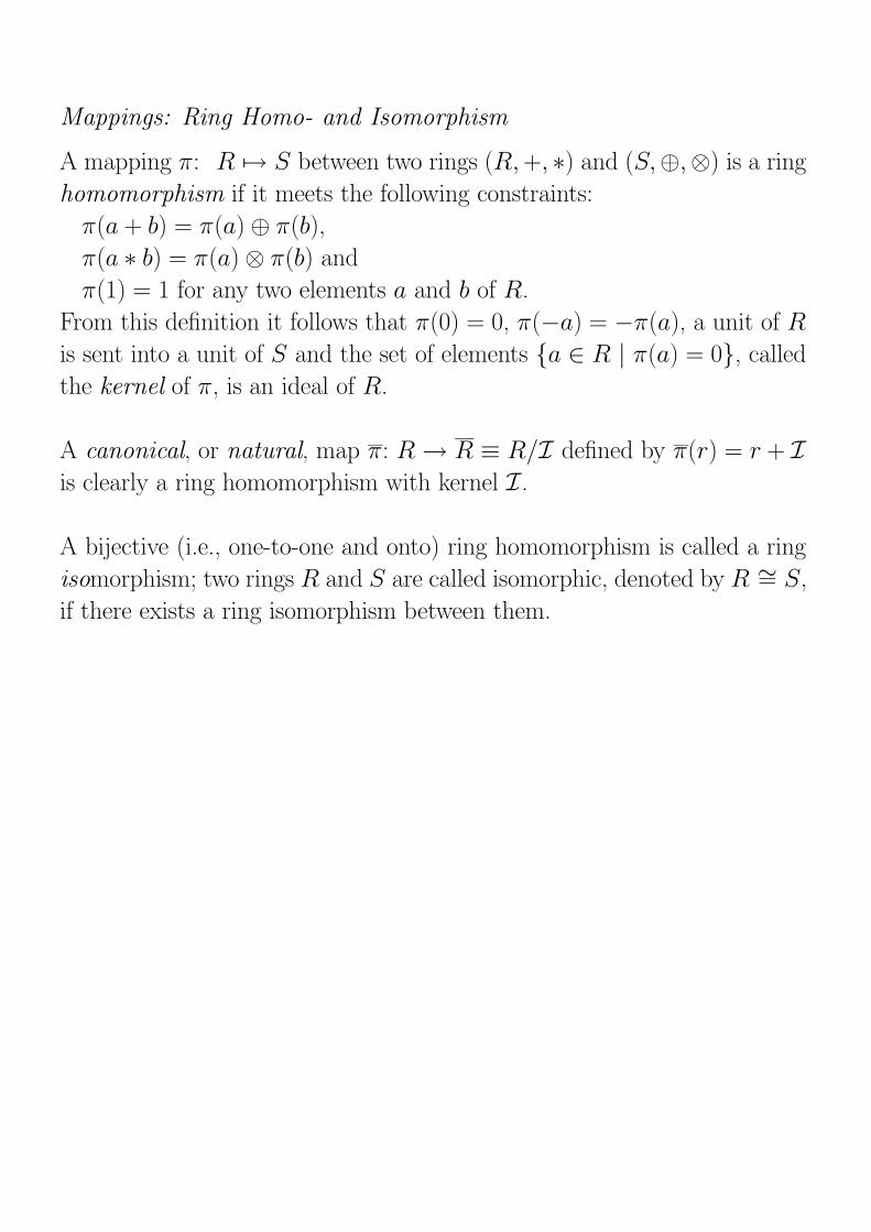
A mapping π: R 7→ S between two rings (R,+, ∗) and (S,⊕,⊗) is a ring
homomorphism if it meets the following constraints:
π(a + b) = π(a)⊕ π(b),
π(a ∗ b) = π(a)⊗ π(b) and
π(1) = 1 for any two elements a and b of R.
From this definition it follows that π(0) = 0, π(−a) = −π(a), a unit of R
is sent into a unit of S and the set of elements {a ∈ R | π(a) = 0}, called
the kernel of π, is an ideal of R.
A canonical, or natural, map π: R→ R ≡ R/I defined by π(r) = r + I
is clearly a ring homomorphism with kernel I.
A bijective (i.e., one-to-one and onto) ring homomorphism is called a ring
isomorphism; two rings R and S are called isomorphic, denoted by R ∼= S,
if there exists a ring isomorphism between them.
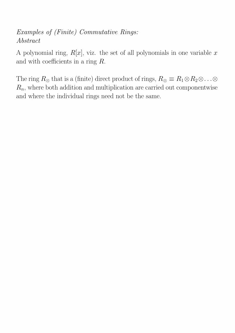
Examples of (Finite) Commutative Rings:
Abstract
A polynomial ring, R[x], viz. the set of all polynomials in one variable x
and with coefficients in a ring R.
The ring R⊗ that is a (finite) direct product of rings, R⊗ ≡ R1⊗R2⊗. . .⊗
Rn, where both addition and multiplication are carried out componentwise
and where the individual rings need not be the same.
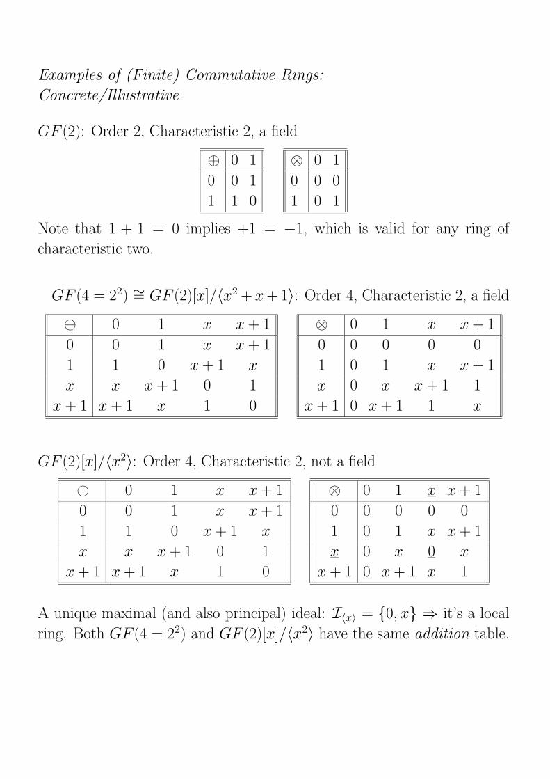
Examples of (Finite) Commutative Rings:
Concrete/Illustrative
GF (2): Order 2, Characteristic 2, a field
⊕ 0 1
0 0 1
1 1 0
⊗ 0 1
0 0 0
1 0 1
Note that 1 + 1 = 0 implies +1 = −1, which is valid for any ring of
characteristic two.
GF (4 = 22) ∼= GF (2)[x]/〈x2 + x+1〉: Order 4, Characteristic 2, a field
⊕ 0 1 x x + 1
0 0 1 x x + 1
1 1 0 x + 1 x
x x x + 1 0 1
x + 1 x + 1 x 1 0
⊗ 0 1 x x + 1
0 0 0 0 0
1 0 1 x x + 1
x 0 x x + 1 1
x + 1 0 x + 1 1 x
GF (2)[x]/〈x2〉: Order 4, Characteristic 2, not a field
⊕ 0 1 x x + 1
0 0 1 x x + 1
1 1 0 x + 1 x
x x x + 1 0 1
x + 1 x + 1 x 1 0
⊗ 0 1 x x + 1
0 0 0 0 0
1 0 1 x x + 1
x 0 x 0 x
x + 1 0 x + 1 x 1
A unique maximal (and also principal) ideal: I〈x〉 = {0, x} ⇒ it’s a local
ring. Both GF (4 = 22) and GF (2)[x]/〈x2〉 have the same addition table.
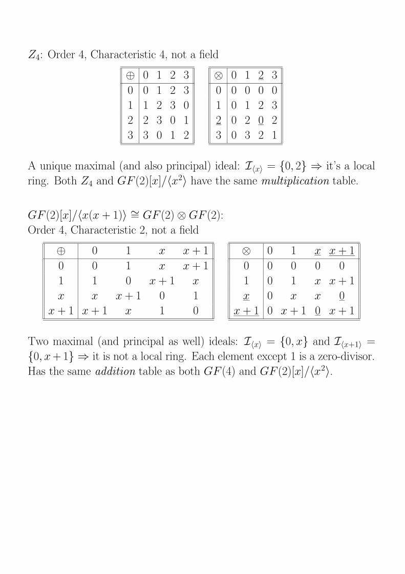
Z4: Order 4, Characteristic 4, not a field
⊕ 0 1 2 3
0 0 1 2 3
1 1 2 3 0
2 2 3 0 1
3 3 0 1 2
⊗ 0 1 2 3
0 0 0 0 0
1 0 1 2 3
2 0 2 0 2
3 0 3 2 1
A unique maximal (and also principal) ideal: I〈x〉 = {0, 2} ⇒ it’s a local
ring. Both Z4 and GF (2)[x]/〈x2〉 have the same multiplication table.
GF (2)[x]/〈x(x + 1)〉 ∼= GF (2)⊗GF (2):
Order 4, Characteristic 2, not a field
⊕ 0 1 x x + 1
0 0 1 x x + 1
1 1 0 x + 1 x
x x x + 1 0 1
x + 1 x + 1 x 1 0
⊗ 0 1 x x + 1
0 0 0 0 0
1 0 1 x x + 1
x 0 x x 0
x + 1 0 x + 1 0 x + 1
Two maximal (and principal as well) ideals: I〈x〉 = {0, x} and I〈x+1〉 =
{0, x+1} ⇒ it is not a local ring. Each element except 1 is a zero-divisor.
Has the same addition table as both GF (4) and GF (2)[x]/〈x2〉.
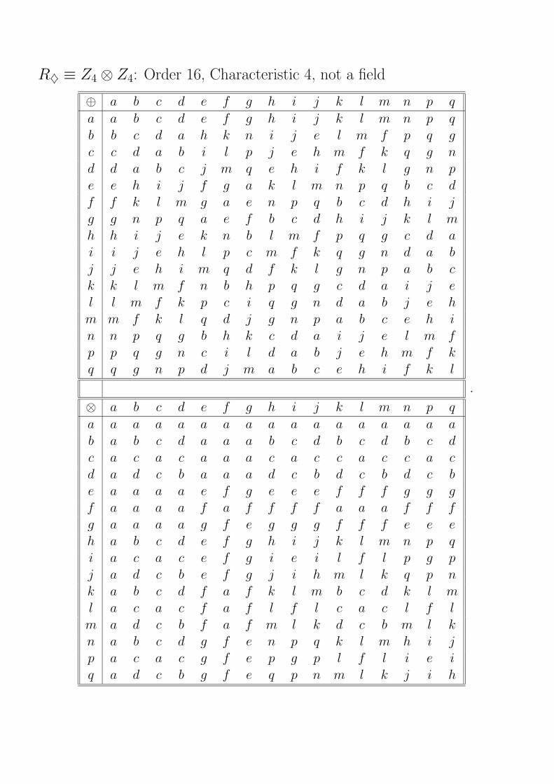
R♦ ≡ Z4 ⊗ Z4: Order 16, Characteristic 4, not a field
⊕ a b c d e f g h i j k l m n p q
a a b c d e f g h i j k l m n p qb b c d a h k n i j e l m f p q g
c c d a b i l p j e h m f k q g nd d a b c j m q e h i f k l g n p
e e h i j f g a k l m n p q b c df f k l m g a e n p q b c d h i j
g g n p q a e f b c d h i j k l mh h i j e k n b l m f p q g c d a
i i j e h l p c m f k q g n d a bj j e h i m q d f k l g n p a b c
k k l m f n b h p q g c d a i j el l m f k p c i q g n d a b j e h
m m f k l q d j g n p a b c e h in n p q g b h k c d a i j e l m f
p p q g n c i l d a b j e h m f kq q g n p d j m a b c e h i f k l
⊗ a b c d e f g h i j k l m n p q
a a a a a a a a a a a a a a a a ab a b c d a a a b c d b c d b c d
c a c a c a a a c a c c a c c a cd a d c b a a a d c b d c b d c b
e a a a a e f g e e e f f f g g gf a a a a f a f f f f a a a f f f
g a a a a g f e g g g f f f e e eh a b c d e f g h i j k l m n p q
i a c a c e f g i e i l f l p g pj a d c b e f g j i h m l k q p n
k a b c d f a f k l m b c d k l ml a c a c f a f l f l c a c l f l
m a d c b f a f m l k d c b m l k
n a b c d g f e n p q k l m h i jp a c a c g f e p g p l f l i e i
q a d c b g f e q p n m l k j i h
.
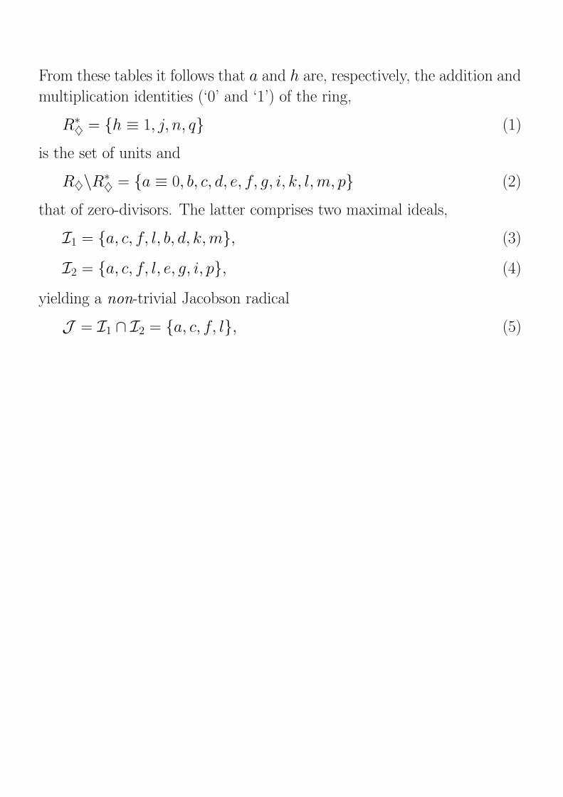
From these tables it follows that a and h are, respectively, the addition and
multiplication identities (‘0’ and ‘1’) of the ring,
R∗♦ = {h ≡ 1, j, n, q} (1)
is the set of units and
R♦\R∗♦ = {a ≡ 0, b, c, d, e, f, g, i, k, l,m, p} (2)
that of zero-divisors. The latter comprises two maximal ideals,
I1 = {a, c, f, l, b, d, k,m}, (3)
I2 = {a, c, f, l, e, g, i, p}, (4)
yielding a non-trivial Jacobson radical
J = I1 ∩ I2 = {a, c, f, l}, (5)

3. Projective Line over a Ring
GL(2, R) and Pair Admissibility
Given
⇒ a ring R with unity and
⇒ GL(2, R), the general linear group of
invertible two-by-two matrices with entries in R,
a pair (α, β) ∈ R2 is called admissible over R if there exist γ, δ ∈ R
such thatα β
γ δ
∈ GL(2, R). (6)
or, equivalently,
det
α β
γ δ
∈ R∗. (7)
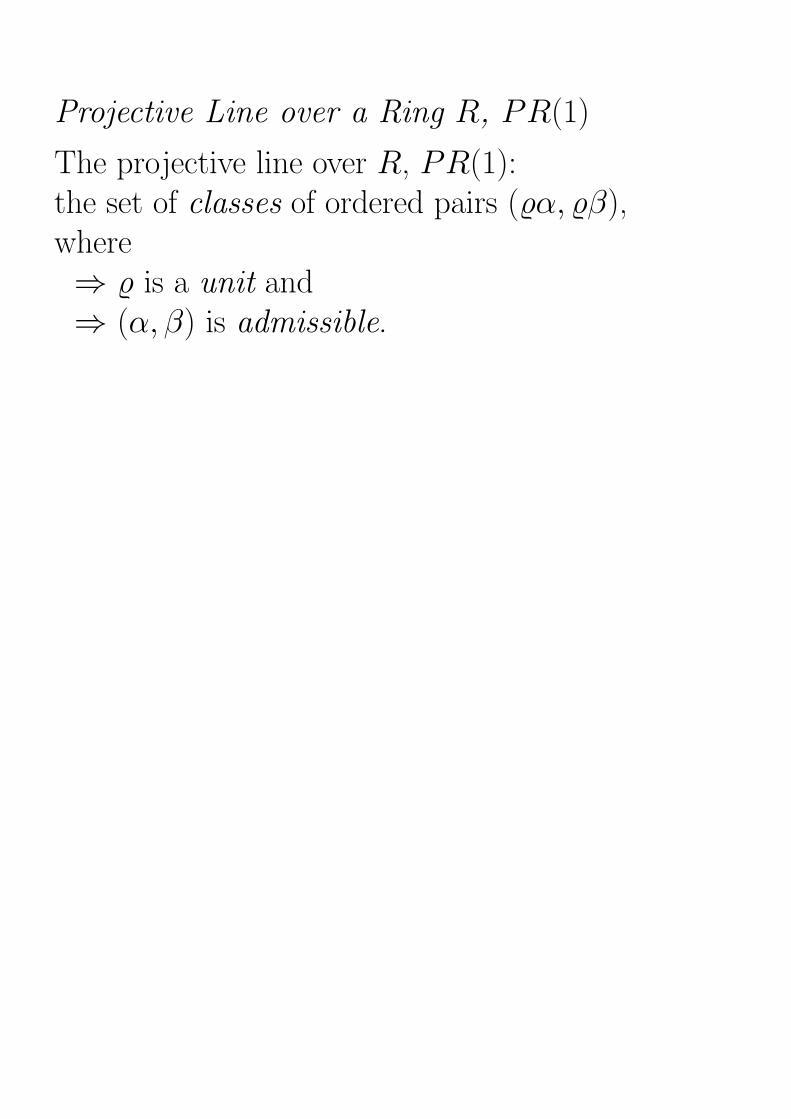
Projective Line over a Ring R, PR(1)
The projective line over R, PR(1):the set of classes of ordered pairs (%α, %β),where⇒ % is a unit and⇒ (α, β) is admissible.
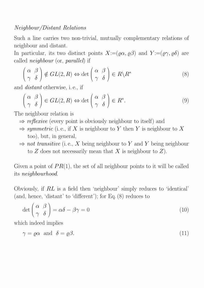
Neighbour/Distant Relations
Such a line carries two non-trivial, mutually complementary relations of
neighbour and distant.
In particular, its two distinct points X :=(%α, %β) and Y :=(%γ, %δ) are
called neighbour (or, parallel) ifα β
γ δ
/∈ GL(2, R)⇔ det
α β
γ δ
∈ R\R∗ (8)
and distant otherwise, i. e., ifα β
γ δ
∈ GL(2, R)⇔ det
α β
γ δ
∈ R∗. (9)
The neighbour relation is
⇒ reflexive (every point is obviously neighbour to itself) and
⇒ symmetric (i. e., if X is neighbour to Y then Y is neighbour to X
too), but, in general,
⇒ not transitive (i. e., X being neighbour to Y and Y being neighbour
to Z does not necessarily mean that X is neighbour to Z).
Given a point of PR(1), the set of all neighbour points to it will be called
its neighbourhood.
Obviously, if RL is a field then ‘neighbour’ simply reduces to ‘identical’
(and, hence, ‘distant’ to ‘different’); for Eq. (8) reduces to
det
α β
γ δ
= αδ − βγ = 0 (10)
which indeed implies
γ = %α and δ = %β. (11)
The Fine Structure of PR(1): Points of Type I and II
PR(1) comprises, in general, two distinct groups of points.
Points of Type I: the points represented by coordinates where
at least one entry is a unit.
It is easy to verify that for any finite commutative ring this number is
always equal to the sum of the total number of elements of the ring and
the number of its zero-divisors; for, indeed,
⇒ if α is a unit then we can always select % in such a way
that (%α, %β) ⇒ (1, β ′), where β ′ ∈ R and
⇒ if β only is a unit then (%α, %β) ⇒ (α′, 1), where α′ ∈ R\R∗.
Points of Type II: the points represented by coordinates where
both entries are zero-divisors.
These points exist only if the ring has two or more maximal ideals and
their number depends on the properties and interconnection between these
ideals. For (%α, %β), with α, β being both zero-divisors of R, to represent
a point of PR(1), Eq. (7) requires
det
α β
γ δ
= αδ − βγ ∈ R∗. (12)
This constraint cannot be met if R contains just a single maximal ideal I,
because α ∈ I implies αδ ∈ I, β ∈ I implies βγ ∈ I, which implies that
the whole expression αδ − βγ ∈ I and, so, is not a unit.
Illustrative Examples of Finite Projective Ring Lines
R = GF (q):
the line contains q (total # of elements) + 1 (# of zero-divisors) points,
any two of them being distant.
R = Z4:
the line contains 4+2 = 6 points, forming three pairs of neighbours, namely
(page 9):
(1, 0) and (1, 2)
(0, 1) and (2, 1)
(1, 1) and (1, 3)
R = GF (2)[x]/〈x(x + 1)〉 ∼= GF (2)⊗GF (2):
the line is endowed with nine points (page 9), out of which there are
seven of the first kind,
(1, 0), (1, x), (1, x + 1), (1, 1),
(0, 1), (x, 1), (x + 1, 1),
and two of the second kind,
(x, x + 1), (x + 1, x).
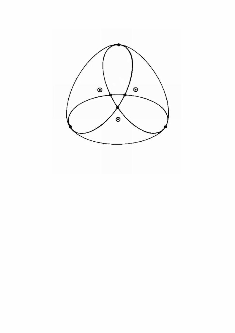
The neighbourhoods of three distinguished pairwise distant points ˜U : (1, 0),
V : (0, 1) and W : (1, 1) here read
˜U : ˜U1 : (1, x), ˜U2 : (1, x + 1), ˜U3 : (x, x + 1), ˜U4 : (x + 1, x), (13)
V : V1 : (x, 1), V2 : (x + 1, 1), V3 : (x, x + 1), V4 : (x + 1, x), (14)
and
W : W1 : (1, x), W2 : (1, x + 1), W3 : (x, 1), W4 : (x + 1, 1). (15)
From these expressions, and the fact that GL(2, R) acts transitively on
triples of mutually distant points, we find that
⇒ the neighbourhood of any point of this line comprises four distinct
points,
⇒ the neighbourhoods of any two distant points have two points in
common (which again implies non-transitivity of the neighbour relation)
and
⇒ the neighbourhoods of any three mutually distant points are disjoint
as illustrated in the figure; note that in this case there exist no “Jacobson”
points, i. e. the points belonging solely to a single neighbourhood, due to
the trivial character of the Jacobson radical, J♣ = {0}.
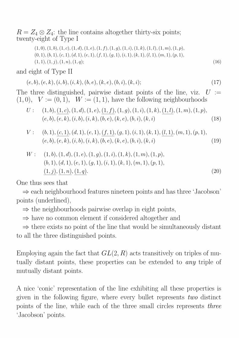
R = Z4 ⊗ Z4: the line contains altogether thirty-six points;twenty-eight of Type I
(1, 0), (1, b), (1, c), (1, d), (1, e), (1, f), (1, g), (1, i), (1, k), (1, l), (1,m), (1, p),
(0, 1), (b, 1), (c, 1), (d, 1), (e, 1), (f, 1), (g, 1), (i, 1), (k, 1), (l, 1), (m, 1), (p, 1),
(1, 1), (1, j), (1, n), (1, q); (16)
and eight of Type II
(e, b), (e, k), (i, b), (i, k), (b, e), (k, e), (b, i), (k, i); (17)
The three distinguished, pairwise distant points of the line, viz. U :=(1, 0), V := (0, 1), W := (1, 1), have the following neighbourhoods
U : (1, b), (1, c), (1, d), (1, e), (1, f), (1, g), (1, i), (1, k), (1, l), (1, m), (1, p),
(e, b), (e, k), (i, b), (i, k), (b, e), (k, e), (b, i), (k, i) (18)
V : (b, 1), (c, 1), (d, 1), (e, 1), (f, 1), (g, 1), (i, 1), (k, 1), (l, 1), (m, 1), (p, 1),
(e, b), (e, k), (i, b), (i, k), (b, e), (k, e), (b, i), (k, i) (19)
W : (1, b), (1, d), (1, e), (1, g), (1, i), (1, k), (1, m), (1, p),
(b, 1), (d, 1), (e, 1), (g, 1), (i, 1), (k, 1), (m, 1), (p, 1),
(1, j), (1, n), (1, q). (20)
One thus sees that
⇒ each neighbourhood features nineteen points and has three ‘Jacobson’
points (underlined),
⇒ the neighbourhoods pairwise overlap in eight points,
⇒ have no common element if considered altogether and
⇒ there exists no point of the line that would be simultaneously distant
to all the three distinguished points.
Employing again the fact that GL(2, R) acts transitively on triples of mu-
tually distant points, these properties can be extended to any triple of
mutually distant points.
A nice ‘conic’ representation of the line exhibiting all these properties is
given in the following figure, where every bullet represents two distinct
points of the line, while each of the three small circles represents three
‘Jacobson’ points.
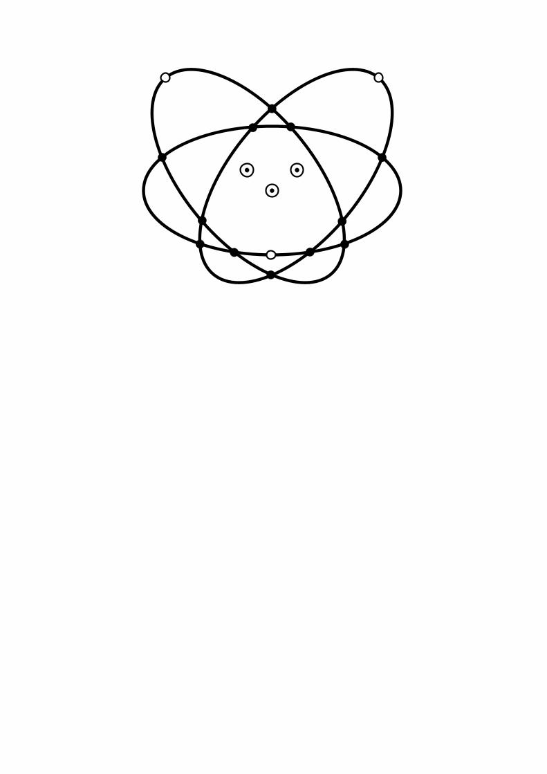
R = GF (2)⊗GF (2)⊗GF (2):
The line possesses twenty-seven points, twelve of Type II; the neighbour-
hood of any point of the line features eighteen distinct points, the neigh-
bourhoods of any two distant points share twelve points and the neigh-
bourhoods of any three mutually distant points have six points in common
— as depicted in the figure.
As in the case of the lines defined over GF(2) ⊗ GF(2) and Z4 ⊗ Z4,
the neighbour relation is not transitive; however, a novel feature, not en-
countered in the previous cases, is here a non-zero overlapping between the
neighbourhoods of three pairwise distant points, which can be attributed
to the existence of three maximal ideals of the ring.
(Every small bullet represents two distinct points of the line, while the big
bullet at the bottom stands for as many as six different points.)
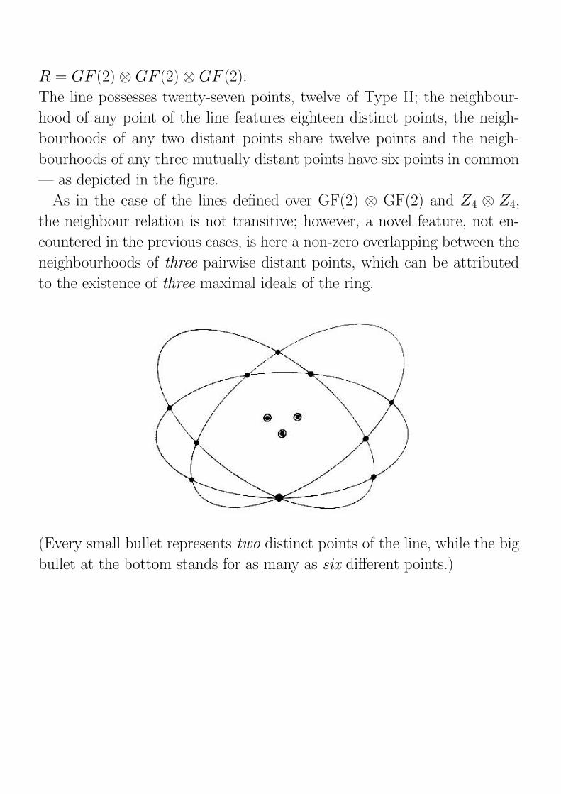
Omitting three distinguished points, the remaining twenty-four points of
the line split into two sets of twelve exhibiting intriguing structures in terms
of the neighbour/distant relation – as illustrated in the figure.

Classification of Projective Ring Lines up to Order 63
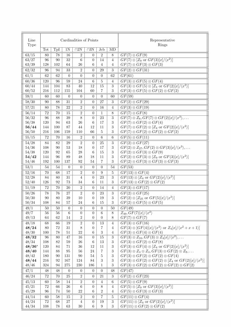
Line Cardinalities of Points RepresentativeType Rings
Tot TpI 1N ∩2N ∩3N Jcb MD
63/15 80 78 16 2 0 2 8 GF (7)⊗GF (9)63/27 96 90 32 6 0 14 4 GF (7)⊗ [Z9 or GF (3)[x]/〈x2〉]63/39 128 102 64 26 6 4 4 GF (7)⊗GF (3)⊗GF (3)
62/32 96 94 33 2 0 29 3 GF (2)⊗GF (31)
61/1 62 62 0 0 0 0 62 GF (61)
60/36 120 96 59 24 6 5 4 GF (3)⊗GF (5)⊗GF (4)60/44 144 104 83 40 12 15 3 GF (3)⊗GF (5)⊗ [Z4 or GF (2)[x]/〈x2〉]60/52 216 112 155 104 60 7 3 GF (3)⊗GF (5)⊗GF (2)⊗GF (2)
59/1 60 60 0 0 0 0 60 GF (59)
58/30 90 88 31 2 0 27 3 GF (2)⊗GF (29)
57/21 80 78 22 2 0 16 4 GF (3)⊗GF (19)
56/14 72 70 15 2 0 1 8 GF (7)⊗GF (8)56/32 96 88 39 8 0 23 3 GF (7)⊗ Z8, GF (7)⊗GF (2)[x]/〈x3〉, . . .56/38 120 94 63 26 6 17 3 GF (7)⊗GF (2)⊗GF (4)56/44 144 100 87 44 12 11 3 GF (7)⊗GF (2)⊗ [Z4 or GF (2)[x]/〈x2〉]56/50 216 106 159 110 66 5 3 GF (7)⊗GF (2)⊗GF (2)⊗GF (2)
55/15 72 70 16 2 0 6 6 GF (5)⊗GF (11)
54/28 84 82 29 2 0 25 3 GF (2)⊗GF (27)54/36 108 90 53 18 0 17 3 GF (2)⊗ Z27, GF (2)⊗GF (3)[x]/〈x3〉, . . .54/38 120 92 65 28 6 15 3 GF (2)⊗GF (3)⊗GF (9)54/42 144 96 89 48 18 11 3 GF (2)⊗GF (3)⊗ [Z9 or GF (3)[x]/〈x2〉]54/46 192 100 137 92 54 7 3 GF (2)⊗GF (3)⊗GF (3)⊗GF (3)
53/1 54 54 0 0 0 0 54 GF (53)
52/16 70 68 17 2 0 9 5 GF (13)⊗GF (4)52/28 84 80 31 4 0 23 3 GF (13)⊗ [Z4 or GF (2)[x]/〈x2〉]52/40 126 92 73 34 6 11 3 GF (13)⊗GF (2)⊗GF (2)
51/19 72 70 20 2 0 14 4 GF (3)⊗GF (17)
50/26 78 76 27 2 0 23 3 GF (2)⊗GF (25)50/30 90 80 39 10 0 19 3 GF (2)⊗ [Z25 or GF (5)[x]/〈x2〉]50/34 108 84 57 24 6 15 3 GF (2)⊗GF (5)⊗GF (5)
49/1 50 50 0 0 0 0 50 GF (49)49/7 56 56 6 0 0 6 8 Z49, GF (7)[x]/〈x2〉49/13 64 62 14 2 0 0 8 GF (7)⊗GF (7)
48/18 68 66 19 2 0 13 4 GF (3)⊗GF (16)48/24 80 72 31 8 0 7 4 GF (3)⊗ [GF (4)[x]/〈x2〉 or Z4[x]/〈x2 + x + 1〉]48/30 100 78 51 22 6 3 4 GF (3)⊗GF (4)⊗GF (4)48/32 96 80 47 16 0 15 3 GF (3)⊗ Z16, GF (3)⊗ Z4[x]/〈x2〉, . . .48/34 108 82 59 26 6 13 3 GF (3)⊗GF (2)⊗GF (8)48/36? 120 84 71 36 12 11 3 GF (3)⊗GF (4)⊗ [Z4 or GF (2)[x]/〈x2〉]48/40 144 88 95 56 24 7 3 GF (3)⊗ Z4 ⊗ Z4, GF (3)⊗GF (2)⊗ Z8, . . .48/42 180 90 131 90 54 5 3 GF (3)⊗GF (2)⊗GF (2)⊗GF (4)48/44 216 92 167 124 84 3 3 GF (3)⊗GF (2)⊗GF (2)⊗ [Z4 or GF (2)[x]/〈x2〉]48/46 324 94 275 230 186 1 3 GF (3)⊗GF (2)⊗GF (2)⊗GF (2)⊗GF (2)
47/1 48 48 0 0 0 0 48 GF (47)
46/24 72 70 25 2 0 21 3 GF (2)⊗GF (23)
45/13 60 58 14 2 0 4 6 GF (5)⊗GF (9)45/21 72 66 26 6 0 8 4 GF (5)⊗ [Z9 or GF (3)[x]/〈x2〉]45/29 96 74 50 22 6 2 4 GF (5)⊗GF (3)⊗GF (3)
44/14 60 58 15 2 0 7 5 GF (11)⊗GF (4)44/24 72 68 27 4 0 19 3 GF (11)⊗ [Z4 or GF (2)[x]/〈x2〉]44/34 108 78 63 30 6 9 3 GF (11)⊗GF (2)⊗GF (2)
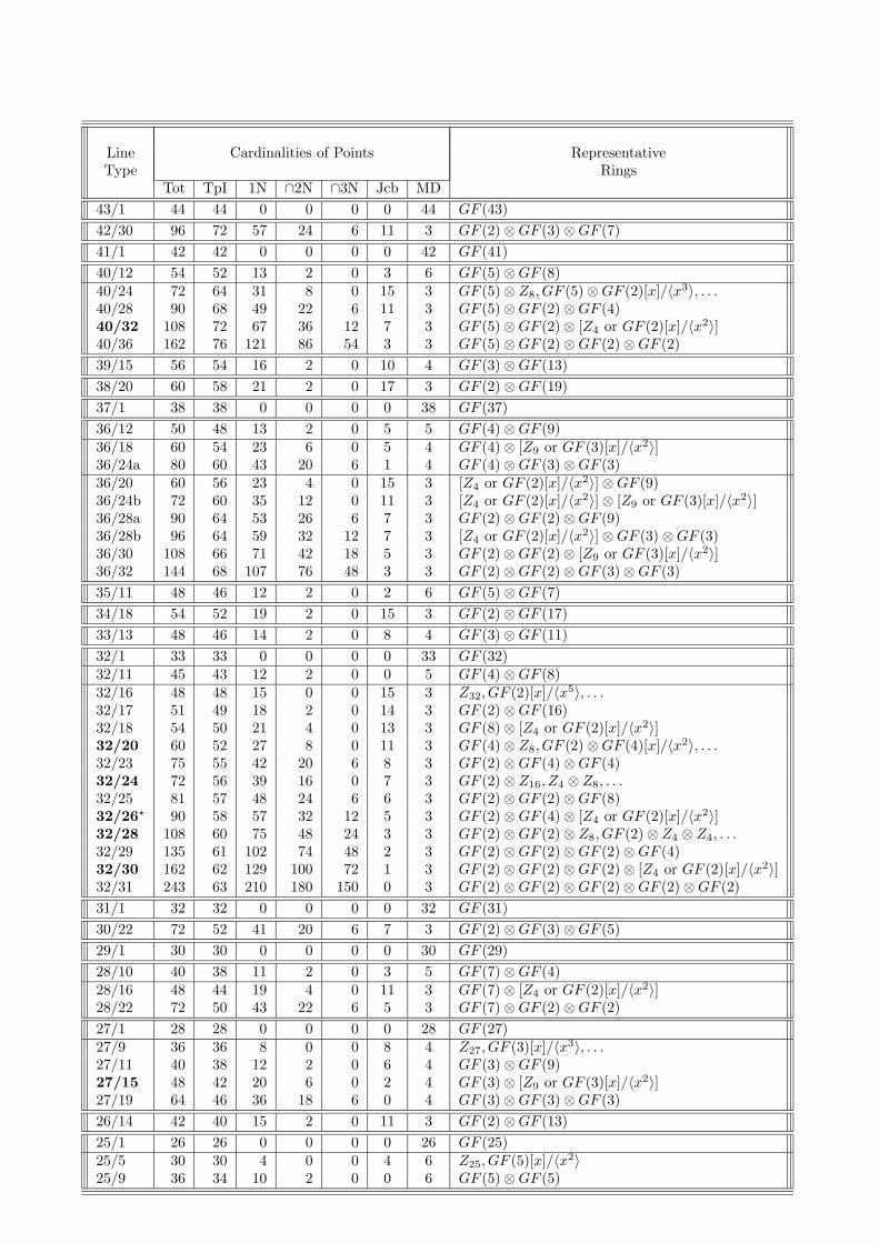
Line Cardinalities of Points RepresentativeType Rings
Tot TpI 1N ∩2N ∩3N Jcb MD
43/1 44 44 0 0 0 0 44 GF (43)
42/30 96 72 57 24 6 11 3 GF (2)⊗GF (3)⊗GF (7)
41/1 42 42 0 0 0 0 42 GF (41)
40/12 54 52 13 2 0 3 6 GF (5)⊗GF (8)40/24 72 64 31 8 0 15 3 GF (5)⊗ Z8, GF (5)⊗GF (2)[x]/〈x3〉, . . .40/28 90 68 49 22 6 11 3 GF (5)⊗GF (2)⊗GF (4)40/32 108 72 67 36 12 7 3 GF (5)⊗GF (2)⊗ [Z4 or GF (2)[x]/〈x2〉]40/36 162 76 121 86 54 3 3 GF (5)⊗GF (2)⊗GF (2)⊗GF (2)
39/15 56 54 16 2 0 10 4 GF (3)⊗GF (13)
38/20 60 58 21 2 0 17 3 GF (2)⊗GF (19)
37/1 38 38 0 0 0 0 38 GF (37)
36/12 50 48 13 2 0 5 5 GF (4)⊗GF (9)36/18 60 54 23 6 0 5 4 GF (4)⊗ [Z9 or GF (3)[x]/〈x2〉]36/24a 80 60 43 20 6 1 4 GF (4)⊗GF (3)⊗GF (3)36/20 60 56 23 4 0 15 3 [Z4 or GF (2)[x]/〈x2〉]⊗GF (9)36/24b 72 60 35 12 0 11 3 [Z4 or GF (2)[x]/〈x2〉]⊗ [Z9 or GF (3)[x]/〈x2〉]36/28a 90 64 53 26 6 7 3 GF (2)⊗GF (2)⊗GF (9)36/28b 96 64 59 32 12 7 3 [Z4 or GF (2)[x]/〈x2〉]⊗GF (3)⊗GF (3)36/30 108 66 71 42 18 5 3 GF (2)⊗GF (2)⊗ [Z9 or GF (3)[x]/〈x2〉]36/32 144 68 107 76 48 3 3 GF (2)⊗GF (2)⊗GF (3)⊗GF (3)
35/11 48 46 12 2 0 2 6 GF (5)⊗GF (7)
34/18 54 52 19 2 0 15 3 GF (2)⊗GF (17)
33/13 48 46 14 2 0 8 4 GF (3)⊗GF (11)
32/1 33 33 0 0 0 0 33 GF (32)32/11 45 43 12 2 0 0 5 GF (4)⊗GF (8)32/16 48 48 15 0 0 15 3 Z32, GF (2)[x]/〈x5〉, . . .32/17 51 49 18 2 0 14 3 GF (2)⊗GF (16)32/18 54 50 21 4 0 13 3 GF (8)⊗ [Z4 or GF (2)[x]/〈x2〉]32/20 60 52 27 8 0 11 3 GF (4)⊗ Z8, GF (2)⊗GF (4)[x]/〈x2〉, . . .32/23 75 55 42 20 6 8 3 GF (2)⊗GF (4)⊗GF (4)32/24 72 56 39 16 0 7 3 GF (2)⊗ Z16, Z4 ⊗ Z8, . . .32/25 81 57 48 24 6 6 3 GF (2)⊗GF (2)⊗GF (8)32/26? 90 58 57 32 12 5 3 GF (2)⊗GF (4)⊗ [Z4 or GF (2)[x]/〈x2〉]32/28 108 60 75 48 24 3 3 GF (2)⊗GF (2)⊗ Z8, GF (2)⊗ Z4 ⊗ Z4, . . .32/29 135 61 102 74 48 2 3 GF (2)⊗GF (2)⊗GF (2)⊗GF (4)32/30 162 62 129 100 72 1 3 GF (2)⊗GF (2)⊗GF (2)⊗ [Z4 or GF (2)[x]/〈x2〉]32/31 243 63 210 180 150 0 3 GF (2)⊗GF (2)⊗GF (2)⊗GF (2)⊗GF (2)
31/1 32 32 0 0 0 0 32 GF (31)
30/22 72 52 41 20 6 7 3 GF (2)⊗GF (3)⊗GF (5)
29/1 30 30 0 0 0 0 30 GF (29)
28/10 40 38 11 2 0 3 5 GF (7)⊗GF (4)28/16 48 44 19 4 0 11 3 GF (7)⊗ [Z4 or GF (2)[x]/〈x2〉]28/22 72 50 43 22 6 5 3 GF (7)⊗GF (2)⊗GF (2)
27/1 28 28 0 0 0 0 28 GF (27)27/9 36 36 8 0 0 8 4 Z27, GF (3)[x]/〈x3〉, . . .27/11 40 38 12 2 0 6 4 GF (3)⊗GF (9)27/15 48 42 20 6 0 2 4 GF (3)⊗ [Z9 or GF (3)[x]/〈x2〉]27/19 64 46 36 18 6 0 4 GF (3)⊗GF (3)⊗GF (3)
26/14 42 40 15 2 0 11 3 GF (2)⊗GF (13)
25/1 26 26 0 0 0 0 26 GF (25)25/5 30 30 4 0 0 4 6 Z25, GF (5)[x]/〈x2〉25/9 36 34 10 2 0 0 6 GF (5)⊗GF (5)
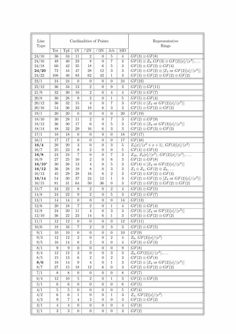
Line Cardinalities of Points RepresentativeType Rings
Tot TpI 1N ∩2N ∩3N Jcb MD
24/10 36 34 11 2 0 5 4 GF (3)⊗GF (8)24/16 48 40 23 8 0 7 3 GF (3)⊗ Z8, GF (3)⊗GF (2)[x]/〈x3〉, . . .24/18 60 42 35 18 6 5 3 GF (3)⊗GF (2)⊗GF (4)24/20 72 44 47 28 12 3 3 GF (3)⊗GF (2)⊗ [Z4 or GF (2)[x]/〈x2〉]24/22 108 46 83 62 42 1 3 GF (3)⊗GF (2)⊗GF (2)⊗GF (2)
23/1 24 24 0 0 0 0 24 GF (23)
22/12 36 34 13 2 0 9 3 GF (2)⊗GF (11)
21/9 32 30 10 2 0 4 4 GF (3)⊗GF (7)
20/8 30 28 9 2 0 1 5 GF (5)⊗GF (4)20/12 36 32 15 4 0 7 3 GF (5)⊗ [Z4 or GF (2)[x]/〈x2〉]20/16 54 36 33 18 6 3 3 GF (5)⊗GF (2)⊗GF (2)
19/1 20 20 0 0 0 0 20 GF (19)
18/10 30 28 11 2 0 7 3 GF (2)⊗GF (9)18/12 36 30 17 6 0 5 3 GF (2)⊗ [Z9 or GF (3)[x]/〈x2〉]18/14 48 32 29 16 6 3 3 GF (2)⊗GF (3)⊗GF (3)
17/1 18 18 0 0 0 0 18 GF (17)
16/1 17 17 0 0 0 0 17 GF (16)16/4 20 20 3 0 0 3 5 Z4[x]/〈x2 + x + 1〉, GF (4)[x]/〈x2〉16/7 25 23 8 2 0 0 5 GF (4)⊗GF (4)16/8 24 24 7 0 0 7 3 Z16, Z4[x]/〈x2〉, GF (2)[x]/〈x4〉, . . .16/9 27 25 10 2 0 6 3 GF (2)⊗GF (8)16/10? 30 26 13 4 0 5 3 GF (4)⊗ [Z4 or GF (2)[x]/〈x2〉]16/12 36 28 19 8 0 3 3 Z4 ⊗ Z4, GF (2)⊗ Z8, . . .16/13 45 29 28 16 6 2 3 GF (2)⊗GF (2)⊗GF (4)16/14 54 30 37 24 12 1 3 GF (2)⊗GF (2)⊗ [Z4 or GF (2)[x]/〈x2〉]16/15 81 31 64 50 36 0 3 GF (2)⊗GF (2)⊗GF (2)⊗GF (2)
15/7 24 22 8 2 0 2 4 GF (3)⊗GF (5)
14/8 24 22 9 2 0 5 3 GF (2)⊗GF (7)
13/1 14 14 0 0 0 0 14 GF (13)
12/6 20 18 7 2 0 1 4 GF (3)⊗GF (4)12/8 24 20 11 4 0 3 3 GF (3)⊗ [Z4 or GF (2)[x]/〈x2〉]12/10 36 22 23 14 6 1 3 GF (3)⊗GF (2)⊗GF (2)
11/1 12 12 0 0 0 0 12 GF (11)
10/6 18 16 7 2 0 3 3 GF (2)⊗GF (5)
9/1 10 10 0 0 0 0 10 GF (9)9/3 12 12 2 0 0 2 4 Z9, GF (3)[x]/〈x2〉9/5 16 14 6 2 0 0 4 GF (3)⊗GF (3)
8/1 9 9 0 0 0 0 9 GF (8)8/4 12 12 3 0 0 3 3 Z8, GF (2)[x]/〈x3〉, . . .8/5 15 13 6 2 0 2 3 GF (2)⊗GF (4)8/6 18 14 9 4 0 1 3 GF (2)⊗ [Z4 or GF (2)[x]/〈x2〉]8/7 27 15 18 12 6 0 3 GF (2)⊗GF (2)⊗GF (2)
7/1 8 8 0 0 0 0 8 GF (7)
6/4 12 10 5 2 0 1 3 GF (2)⊗GF (3)
5/1 6 6 0 0 0 0 6 GF (5)
4/1 5 5 0 0 0 0 5 GF (4)4/2 6 6 1 0 0 1 3 Z4, GF (2)[x]/〈x2〉4/3 9 7 4 2 0 0 3 GF (2)⊗GF (2)
3/1 4 4 0 0 0 0 4 GF (3)
2/1 3 3 0 0 0 0 3 GF (2)
4. Conclusion/References
Saniga, M., Planat, M., and Pracna, P.: 2006, A Classification of the ProjectiveLines over Small Rings II. Non-Commutative Case, to be submitted;(http://hal.ccsd.cnrs.fr/ccsd-00080736 and http://arXiv.org/abs/math.AG/0606500).
Planat, M., Saniga, M., and Kibler, M. R.: 2006, Quantum Entanglement andProjective Ring Geometry, SIGMA, accepted; (http://hal.ccsd.cnrs.fr/ccsd-00077093and http://arXiv.org/abs/quant-ph/0605239).
Saniga, M., Planat, M., Kibler, M. R., and Pracna, P.: 2006, A Classification of theProjective Lines over Small Rings, submitted; (http://hal.ccsd.cnrs.fr/-ccsd-00068327and http://arXiv.org/abs/math.AG/0605301).
Saniga, M., and Planat, M.: 2006, On the Fine Structure of the Projective Lineover GF(2) ⊗ GF(2) ⊗ GF(2), submitted; (http://hal.ccsd.cnrs.fr/ccsd-00022719 andhttp://arXiv.org/abs/math.AG/0604307).
Saniga, M., Planat, M., and Minarovjech, M.: 2006, The Projective Line over theFinite Quotient Ring GF(2)[x]/〈x3 − x〉 and Quantum Entanglement II. The Mermin“Magic” Square/Pentagram, submitted; (http://hal.ccsd.cnrs.fr/ccsd-00021604 andhttp://arXiv.org/abs/quant-ph/0603206).
Saniga, M., and Planat, M.: 2006, The Projective Line over the Finite Quotient RingGF(2)[x]/〈x3 − x〉 and Quantum Entanglement I. Theoretical Background, submitted;(http://hal.ccsd.cnrs.fr/ccsd-00020182 and http://arXiv.org/abs/quant-ph/0603051).
Saniga, M., and Planat, M.: 2006, Finite Geometries in Quantum Theory: From Ga-lois (Fields) to Hjelmslev (Rings), International Journal of Modern Physics B, 20(11–13), 1885–1892.
Saniga, M., and Planat, M.: 2006, Projective Planes over “Galois” Double Num-bers and a Geometrical Principle of Complementarity, Chaos, Solitons & Fractals, inpress; (http://hal.ccsd.cnrs.fr/ccsd-00016658 and http://arXiv.org/abs/math.NT/-0601261).
Saniga, M., and Planat, M.: 2006, Hjelmslev Geometry of Mutually Unbiased Bases,Journal of Physics A: Mathematical and General, 39(2), 435–440;(http://hal.ccsd.cnrs.fr/ccsd-00005539 and http://arXiv.org/abs/math-ph/0506057).


![A survey on projectively equivalent representations of finite groups · The theory of projective representations of finite groups was founded by I. Schur [25] and the notion of projective](https://static.fdocuments.us/doc/165x107/5f0db3177e708231d43ba5cb/a-survey-on-projectively-equivalent-representations-of-finite-the-theory-of-projective.jpg)