Csaba Mengyán CONSTRUCTIONAL METHODS IN FINITE PROJECTIVE ...web.cs.elte.hu/phd_th/mengyan.pdf ·...

Csaba Mengyán

CONSTRUCTIONAL METHODS IN FINITEPROJECTIVE GEOMETRY

PhD thesis

Supervisor: Prof. Tamás Szőnyi

Mathematics PhD School of the Eötvös Loránd University

Director: Prof. Miklós Laczkovich

Pure Mathematics PhD Program

Director: Prof. János Szenthe

Department of Computer Science, Eötvös Loránd University,Budapest, Hungary

2008

Contents

Preambulum 3Overview . . . . . . . . . . . . . . . . . . . . . . . . . . . . . . . . . 3Acknowledgement . . . . . . . . . . . . . . . . . . . . . . . . . . . . . 5Notation . . . . . . . . . . . . . . . . . . . . . . . . . . . . . . . . . . 6

1 Introduction 91.1 Basic definitions . . . . . . . . . . . . . . . . . . . . . . . . . . . 9

1.1.1 Minimal blocking set . . . . . . . . . . . . . . . . . . . . 91.1.2 Unital and Hermitian curve . . . . . . . . . . . . . . . . 101.1.3 High dimensional structures . . . . . . . . . . . . . . . . 10

1.2 Upper and lower bounds . . . . . . . . . . . . . . . . . . . . . . 111.3 The spectrum . . . . . . . . . . . . . . . . . . . . . . . . . . . . 161.4 Related notions . . . . . . . . . . . . . . . . . . . . . . . . . . . 171.5 Constructional methods . . . . . . . . . . . . . . . . . . . . . . 18

1.5.1 Embeddings . . . . . . . . . . . . . . . . . . . . . . . . . 181.5.2 Partitioning with curves . . . . . . . . . . . . . . . . . . 191.5.3 Random Choice . . . . . . . . . . . . . . . . . . . . . . . 191.5.4 Adding and deleting points . . . . . . . . . . . . . . . . . 201.5.5 The Rédei construction, subsets and cosets . . . . . . . . 21

1.6 Weil’s theorem and its variants . . . . . . . . . . . . . . . . . . 22

2 Constructions in space 252.1 The André, Bruck-Bose representation . . . . . . . . . . . . . . 252.2 A general cone construction . . . . . . . . . . . . . . . . . . . . 262.3 The generalized Buekenhout construction . . . . . . . . . . . . . 28

1

2 CONTENTS

2.4 Some more results . . . . . . . . . . . . . . . . . . . . . . . . . . 322.5 Partitioning the flags . . . . . . . . . . . . . . . . . . . . . . . . 33

2.5.1 The trivial estimate . . . . . . . . . . . . . . . . . . . . . 332.5.2 The Illés, Szőnyi, Wettl method . . . . . . . . . . . . . . 342.5.3 The embedding method . . . . . . . . . . . . . . . . . . 36

3 Constructions in the plane 413.1 Random constructions in the plane . . . . . . . . . . . . . . . . 41

3.1.1 The parabola construction . . . . . . . . . . . . . . . . . 413.1.2 Blocking sets arising from a Hermitian curve . . . . . . . 44

3.2 The method of subsets and cosets . . . . . . . . . . . . . . . . . 473.2.1 Blocking sets from a triangle . . . . . . . . . . . . . . . . 473.2.2 Megyesi’s construction . . . . . . . . . . . . . . . . . . . 51

4 A generalization of Megyesi’s construction 554.1 Placing cosets on three lines . . . . . . . . . . . . . . . . . . . . 564.2 Embedding and non-Rédei minimal blocking sets . . . . . . . . 60

Bibliography 65

Summary 71

Magyar nyelvű összefoglaló 73

Preambulum

Overview

In finite projective geometry several methods both from geometry and algebracan be used to attain new results. In this thesis we concentrate on some methodsof particular importance in the construction of minimal blocking sets and aclosely related notion, strong representative systems.

The preambulum is devoted to an overview of the thesis, acknowledgementand notation.

In Chapter 1 we give some basic definitions and concepts. We prove ageneralization of the Bruen-Thas upper bound in Section 1.2. In Section 1.5 wegive a short overview of the methods to be discussed: embedding, partitioning,random choice, adding and deleting points and use of subsets. The descriptionhere is very general, but in subsequent chapters we provide ample examples oftheir uses. We also include a strong algebraic technical tool, Weil’s estimateand some of its variants.

Chapter 2 is devoted to higher dimensional constructions using embeddingand partitioning. In Sections 2.1 and 2.2 we give necessary definitions and ageneral construction. In Section 2.3 we describe the generalized Buekenhoutconstruction, and a particular type of large minimal blocking set obtained usingthis embedding method. In Section 2.4 we present some results obtained bythe generalized Buekenhout construction and its modifications. In subsectionsof Section 2.5 we show three solutions to a problem raised by Gyárfás that isequivalent to partitioning the flags of PG(2, q) into strong representative sys-tems. The first two subsections give results using geometrical and partitioningarguments, while the last part of the chapter shows a solution to this problem

3

4 PREAMBULUM

obtained by the generalized Buekenhout construction using minimal blockingsets described in Section 2.3, and demonstrates the power of the embeddingmethod over the other solutions.

In Chapter 3 we consider constructions in the plane. The results here userandom choice in the first part of the chapter, and mainly subsets and cosetsin the second part. In Section 3.1 we show density results and that the numberof such structures is in most cases more than polynomial, a question originallyasked by Turán. In Section 3.2 we construct more than polynomial numberof minimal blocking sets starting from the well-known triangle and Megyesi’sexample respectively by placing suitable subsets (of points) on lines.

In Chapter 4 we investigate Megyesi’s example more thoroughly. In Section4.1 we show a generalization of Megyesi’s example, and prove that there is astrong correspondence between such constructions and some trivial equations.Finally, in Section 4.2 we introduce a simple embedding method and sketchanother high dimensional embedding method, and discuss their implications toconstructing non-Rédei minimal blocking sets.

Finally, we end the thesis with the Bibliography, Summary and Hungariansummary.

5

Acknowledgement

Above all, I am thankful to my supervisor and menthor, professor Tamás Szőnyi,who had introduced me to finite geometry in the first place, and who made mystudies of this field possible and also successful.

I am very grateful to professor Andrács Gács, who was instrumental in pro-viding help and guidance to me in writing the articles that this thesis is basedon.

I would also like to thank my co-authors: M. Nóra Viola Harrach and ZsuzsaWeiner for the joint work, and everyone at the Computer Science Departmentof the Eötvös Loránd University for being very helpful throughout my researchperiod there.

6 PREAMBULUM

Notation

Finite Desarguesian projective spaces PG(n, q) are all formed from the under-lying Galois fields GF(q). Hence q is a power of p, where p is prime.

Let Vn+1 be the (n + 1)-dimensional vector space over GF(q) with origin O.Consider the following relation on Vn+1 \ {O}: elements x = (x1, x2, ..., xn+1)

and y = (y1, y2, ..., yn+1) are in relation if there is a 0 6= λ ∈ GF(q) for whichxi = λyi for every i = 1, 2, ..., n + 1. This is an equivalence relation, andthe equivalence classes correspond to the 1-dimensional subspaces of Vn+1, thepoints of PG(n, q). A point is represented by any of the vectors from the givenequivalence class. (The set of equivalence classes is the set of points of PG(n, q)).

An m-dimensional subspace or m-space of PG(n, q) is the set of points allof whose representing vectors form (together with the origin) a subspace ofdimension m + 1 of Vn+1. A subspace of dimension zero has already beencalled a point; subspaces of dimension one and two are called line and planerespectively. Subspaces of dimension n− 1 are called hyperplanes. Hyperplanesare represented similarly to the points by n-tuples. A point is incident with ahyperplane if and only if the scalar product of their coordinate vectors is zero.

Throughout this paper we will work in the finite Desarguesian projectivespace PG(n, q) and its affine part AG(n, q). The order of the space (plane) isq. For these spaces (planes) standard representations will be used, see [26].

The points of AG(2, q) have affine coordinates, represented by pairs, wherethe elements of the pairs are elements of GF(q). The lines of AG(2, q) haveequation mX + b − Y = 0 or X = c, where m is the slope of the line. Theinfinite points can be identified with slopes, so (m) defines the infinite point oflines with slope m. In the same way (∞) will be the infinite point of the verticallines, that is the lines with equation X = c. Instead of infinite the term ideal isalso used in the text. The ideal points together with AG(2, q) are the projectiveclosure of AG(2, q), which is PG(2, q) defined above.

For vectors we use boldface letters. If x = (x1, x2, .., xn) then by xb wemean x = (xb

1, xb2, ..., x

bn). The same applies for the notation of matrices H, the

exponent is considered elementwise (for each entry in the matrix).

In this paper for the multiplicative subgroup of GF(q) we use the notation

7

(GF(q), ·). Finally, we note that blocking sets are usually denoted by B, someother sets linked to blocking sets by S and ovoids by O. Generally (but notalways), capital letters stand for points, lower case letters for lines and greekletters for spaces.

The thesis tries to follow the usual notation found in the literature.

8 PREAMBULUM

Chapter 1

Introduction

1.1 Basic definitions

1.1.1 Minimal blocking set

A blocking set in a projective plane is a set of points which intersects everyline. Lines that intersect the blocking set B in exactly one point of B are calledtangents. A line intersecting B in k points (k > 0) is called a k-secant or simplya secant. A point P of a blocking set B is called essential, if B \ {P} is not ablocking set. Geometrically, a point is essential if there is a tangent line at P ,that is, a line intersecting B just at P . A blocking set is said to be minimal,when no proper subset of it is a blocking set, or, equivalently if each point ofthe blocking set is essential. Note that a minimal blocking set in a projectiveplane is either a line, or does not contain a line. A blocking set is called trivialif it contains all points from a line. It is straightforward to check that lines arethe smallest blocking sets. If there is exactly one tangent t to B at P , then P iscalled a critical point, and t a critical tangent. Blocking sets for which there isa line l such that |B \ l| = q are said to be Rédei blocking sets (or blocking setsof Rédei-type). Such a line l is called a Rédei line of the blocking set. Blockingsets are also characterized by their sizes; a blocking set is small if its size is lessthan 3(q + 1)/2, and large if its size is greater than 3q − 3. Note that in thisthesis we mainly investigate blocking sets in the plane, which are also calledplanar blocking sets.

9

10 CHAPTER 1. INTRODUCTION

1.1.2 Unital and Hermitian curve

A pointset U of PG(2, q) is called a unital if it has q√

q+1 points, and every lineintersects it in 1 or √q + 1 points. The Hermitian curve is a classical unital; itis a curve projectively equivalent to the curve defined by the following equation:

X√

q+10 + X

√q+1

1 + X√

q+12 = 0

or equivalently in matrix form,

x√

qHxT = 0

such that H = (H√

q)T is a Hermitian matrix.The set H of points of such a curve form a unital, that is, its size is q

√q + 1

and it meets every line in 1 or √q +1 points. (We shall call these lines tangentsand secants, respectively.)

There is a unique tangent at each point of H, while through a point not onthe curve there are √q + 1 tangents.

Tangents through a point P /∈ H meet H in collinear points, the correspond-ing secant is called the polar of P and denoted by P⊥, and vice versa, tangentsat points of a secant ` are concurrent at a point called the pole of ` and denotedby `⊥.

All secants meet the curve in a Baer subline. The Baer sublines PG(1, q) ofPG(1, q2) form the blocks of a 3−(q2 +1, q+1, 1) design, that is an inversive (orMöbius) plane. This means that three points determine a unique Baer subline,and two sublines meet in at most two points.

1.1.3 High dimensional structures

An embedding is an injective (one-to-one) mapping, where the (original) inci-dence properties are invariant under the mapping.

A projective space PG(n, q) embedded in PG(n, qk) is called a subgeometry.When n = 2 it is called a subplane and when k = 2 it is the Baer subgeometryof dimension n. For n = k = 2 they are the Baer subplanes.

1.2. UPPER AND LOWER BOUNDS 11

A blocking set with respect to k-dimensional subspaces in PG(n, q) is a setB of points which intersects every k-dimensional subspace. Sometimes they arecalled k-blocking sets.

An oval is a set of points that every line meets in 0,1 or 2 points such thatthere is exactly one tangent at each of its points.

A spread of PG(n, q) is a set F of r-dimensional subspaces of PG(n, q), ifthe elements of F partition the points of PG(n, q).

An ovoid O is a set of q2 points in PG(3, q) such that no three points ofO are on the same line of PG(3, q). We will only consider classical ovoids (i.e.non-singular elliptic quadrics Q3) in PG(3, q) that have q2 + 1 points. Thesehave canonical equation Q3 = F (x1, x2) + x3x4 for some coordinate system,where F is an irreducible quadratic polynomial.

Consider three subspaces of PG(n, q), namely γ, π and a subspace V disjointboth from γ and π. Then by a projection of a point P ∈ γ from V onto π wemean the unique intersection of π and the space spanned by P and V , 〈P, V 〉.By a projection of γ from V onto π we mean the pointwise projection of γ.

Consider two disjoint subspaces π and V in a projective space. Let O be asubstructure contained entirely in π. A cone with base O and vertex V is theunion of the connecting lines (considered as a pointset) of the points of O tothe points of V .

1.2 Upper and lower bounds

Here we are going to discuss the minimal and maximal sizes a minimal blockingset can have in the plane. For q = 2 we have the Fano plane, and as Neumannand Morgenstern observed in the 1940’s there are no minimal blocking sets inthis case. Therefore, we always consider q to be greater than 2.

A lower bound for the size of minimal blocking sets was given by Bruen [17]and Pelikán.

Theorem 1.1 (Bruen and Pelikán, [17]) Non-trivial minimal blocking sets ofPG(2, q) contain at least q+

√q+1 points. If there is equality, then the minimal

blocking set is a Baer subplane.


Theorem 1.1 is combinatorial, that is it holds for any projective plane oforder q > 2. There are much better lower bounds when q is not a square andthe plane is Desarguesian.

Theorem 1.2 (Blokhuis, [8]) If q is a prime, then the size of a non-trivialblocking set is at least 3(q+1)

2. If q = ph is neither a square nor a prime, then

the size of a non-trivial blocking set is at least q +√

pq + 1.

The lower bound was further improved by Blokhuis, Storme and Szőnyi [15].

Theorem 1.3 (Blokhius, Storme, Szőnyi, [15]) If q = ph, h is odd, then |B| ≥q + 1 + cpq

2/3, where c2 = c3 = 2−1/3 and cp = 1 for p > 3.

Theorem 1.4 (Szőnyi, [41]) Let B be a non-trivial minimal blocking set inPG(2, q), q = pn. Suppose that |B| < 3(q + 1)/2. Then

q + 1 +q

pe + 2≤ |B| ≤

qpe + 1−√

(qpe + 1)2 − 4q2pe

2,

for some integer e, 1 ≤ e.

In the particular case when q = p2, the previous theorem has the followingcorollary.

Corollary 1.5 Let q = p2 and B be a non-trivial minimal blocking set which isnot a Baer subplane. Then |B| ≥ 3(q + 1)/2.

The result about the intervals was improved by Sziklai [40], who showed thatonly the intervals with e|n are nonempty. He also proved that the (pe+1)-secantsof the blocking set are sublines.

An upper bound for the size of minimal blocking sets was given by Bruenand Thas [19].

Theorem 1.6 (Bruen and Thas, [19]) If B is a minimal blocking set of PG(2, q)

then |B| ≤ q√

q + 1. In case of equality B is a unital (and q is square).


Proof. Let t be the number of tangents of B, and consider the non-tangentlines: L1, ..., LN , where N = q2 + q + 1 − t. Let nj = |Lj ∩ B|, j = 1, ..., N .Counting the pairs (point of B, lines through this point) and (a pair of pointsof B, connecting lines through these points) we get that

∑nj = |B|(q + 1)− t

and∑

nj(nj − 1) = |B|(|B| − 1). Summing these two equations gives∑

n2j =

|B|2 + |B|q − t. Using the inequality between the geometric and arithmeticmeans gives

NN∑

j=1

n2j ≥ (

N∑j=1

nj)2

that is (q2 + q + 1− t)(|B|2 + |B|q − t)− (|B|q + |B| − t)2 ≥ 0.Some easy calculations give (|B|2 + q2 + q +1−|B|q− 2|B|)t−|B|(q3 + q2 +

q − |B|q) ≤ 0.As B is minimal t ≥ |B|, and the coefficient of t is positive. Replacing t by

|B| still gives the calculated inequality. Rearranging gives then |B| ≤ q√

q + 1.In case of equality t = |B| and every non-tangent line meets B in exactly √q+1

points.

An improvement on the Bruen-Thas upper bound is possible, as we nowshow, see [4].

Theorem 1.7 (Szőnyi, Cossidente, Gács, Mengyán, Siciliano, Weiner, [4])Suppose B is a minimal blocking set in PG(2, q), q 6= 5, and denote by s the

fractional part of √q. Then |B| ≤ q√

q + 1− 14s(1− s)q.

Note that this always implies at least a 1/8√

q improvement on the Bruen–Thas upper bound. On the other hand, it is easy to see that if q is not too closeto a square, then this implies a cq improvement.

Before the proof of Theorem 1.7, we need a lemma, which is also used in theproof of Turán’s theorem on graphs containing no Kr (see Lovász, [33]).

Lemma 1.8 Let a1, ..., an be integers with a1+...+an = N . Then a21+...+a2

n ≥N(2α + 1) − nα(α + 1), where α denotes the integer part of N/n. If equalityholds, then all the ais are the same or they take two different values accordingas N/n is an integer or not.


Proof. Note that (a− 1)2 +(b+1)2 < a2 + b2 whenever a > b+1. This showsthat if we have integers a1, ..., an taking at least three values, we can decrease thesum of their squares (without changing their sum) by changing an appropriatelychosen pair (ai, aj) to (ai−1, aj +1). So starting with a1 = N, a2 = ... = an = 0,after finitely many steps we end up with a multiset {a1, ..., an} consisting of atmost two values, α and α + 1. It is easy to see that if N/n is integer, then wecan only have one value, which is N/n; while for N/n non-integer, α has to bethe integer part of N/n.

If we know that the multiset {a1, ..., an} consists of α-s and (α + 1)-s, wecan determine the number k of α-s using the equation kα+(n−k)(α+1) = N .This gives k = n(α + 1) − N , hence the minimum is kα2 + (n − k)(α + 1)2 =

N(2α + 1)− nα(α + 1).

Proof of Theorem 1.7 The proof works only for q ≥ 53, for smaller valuessee the remark after the proof.

Write b = |B| = q√

q+1−ε and let r = [√

q], the integer part of√q. From theBruen–Thas upper bound we know that ε > 0, we need ε ≥ 1/4s(1−s)q. Denoteby a1, ..., aq2+q+1 the intersection sizes of B with lines. Since B is minimal, wecan suppose that a1 = · · · = ab = 1. From standard double counting, we find

q2+q+1∑i=b+1

ai = b(q + 1)− b = bq; (1.1)

q2+q+1∑i=b+1

ai(ai − 1) = b(b− 1). (1.2)

Finally, the sum of these two equations gives

q2+q+1∑i=b+1

a2i = b(b− 1 + q). (1.3)

We wish to use Lemma 1.8. Here n = q2 + q + 1 − b and N = bq. N/n =bq

q2+q+1−b= q

(q2+q+1)/b−1is increasing in b and for b = q

√q + 1 it is √q + 1, so

N/n <√

q + 1. We prove that if N/n ≤ r + 1, then b ≤ q√

q + 1− 14s(1− s)q

automatically holds, so α = [N/n] = r + 1 can be supposed.


N/n ≤ r + 1 is equivalent to b ≤ (r+1)(q2+q+1)q+r+1

. We need that the right handside is at most q

√q+1−1/4s(1−s)q. We consider the even stronger inequality

(r + 1)(q2 + q + 1)

q + r + 1≤ q

√q + 1− 1/4sq.

Replacing r with √q − s and after a little calculation we find the following

equivalent form:

0 ≤ sq(3/4q − 5/4√

q + 3/4 + 1/4s2),

this is true for q ≥ 53.Now Lemma 1.8 and (1.3) imply that

b(b− 1 + q) ≥ (2r + 3)bq − (q2 + q + 1− b)(r + 1)(r + 2).

Replacing r with √q − s and after a little manipulation, we find

b2 − (2q√

q + 3q + 3√

q + 3)b + (q2 + q + 1)(q + 3√

q + 2)+

+s(2q + 2√

q + 3− s)b− s(q2 + q + 1)(2√

q + 3− s) ≥ 0,

which is equivalent to

(b− q√

q − 1)(b− q√

q − 3q − 3√

q − 2)

−s{(q2 + q + 1)(2√

q + 3− s)− (2q + 2√

q + 3− s)b} ≥ 0.

Hence

ε = q√

q + 1− b ≥ s(q2 + q + 1)(2

√q + 3− s)− (2q + 2

√q + 3− s)b

q√

q + 3q + 3√

q + 2− b=

2s(√

q + 1)(q2 + q + 1)− (q +√

q + 1)b

q√

q + 3q + 3√

q + 2− b+ s(1− s)

q2 + q + 1− b

q√

q + 3q + 3√

q + 2− b.

Replacing b with q√

q + 1− ε and after some calculation, we find

ε ≥ 2sε(q +

√q + 1)

3(q +√

q + 1) + ε− 2+ s(1− s)

q2 + q + 1− q√

q − 1 + ε

3q + 3√

q + 1 + ε.(1.4)


Now the best we can get from ε ≥ 14s(1 − s)q is q

16, so we can suppose ε ≤ q

16.

After this, an easy calculation shows that, if q ≥ 49 holds, then the secondterm on the right hand side of (1.4) is at least s(1− s) q

4. Since the first one is

non-negative, we are done.

Remark 1.9 For q < 53, a case by case application of Lemma 1.8 yields theresult of Theorem 1.7. Furthermore, the direct use of the lemma gives slightlybetter bounds in several cases. For q = 5, the union of three lines minus theintersection points is a blocking set of size 12, showing that in this case theBruen–Thas upper bound is tight.

Remark 1.10 Note that the proof of Theorem 1.7 is combinatorial, so the resultis true for any projective plane of order q ≥ 53. Again using Lemma 1.8 directly,all values less than 53 can be ruled out except for 26.

1.3 The spectrum

Under the term spectrum we mean a characterization of blocking sets (or otherstructures) with respect to their sizes. As already described previously: thesmallest size for a blocking set in PG(2, q) after q + 1 (the size of a line) isq+

√q+1 with equality if and only if q is square and the set is a Baer subplane,

and the biggest possible size is q√

q + 1 with equality if and only if q is squareand the set is a unital. The spectrum can be divided into four major parts, intothe following intervals:

I. [q +√

q + 1, 3(q+1)2

) (small minimal blocking sets)

II. [3(q+1)2

, 2q − 2]

III. [2q − 1, 3q − 3]

IV. (3q − 3, q√

q + 1] (large minimal blocking sets)

The reason the intervals are divided like this is mainly due to the differentpossible techniques and approaches connected to them. Small minimal blocking

1.4. RELATED NOTIONS 17

sets are partly characterized, for blocking sets from the second interval mainlyconstructions are known. In the third interval there is a minimal blocking setfor all sizes, while large minimal blocking sets are rare.

There are several survey papers about blocking sets. (See Blokhuis [9], [10],Szőnyi, Gács, Weiner [45], and Chapter 13 of the second edition of Hirschfeld’sbook [26] also contains a lot of recent results).

1.4 Related notions

A tangency set S is a set of points such that every point P ∈ S has a tangent,in other words there exists a line l at P such that S ∩ l = {P}. The tangenyset S is maximal if no further point can be added to it preserving the tangencyproperty; that is none of whose supersets are tangency sets [18].

Minimal blocking sets are all maximal tangency sets. The notion of maximaltangency sets is more general than that of minimal blocking sets as was shownin [18], because for q even, an oval is a maximal tangency set, but clearly not aminimal blocking set. Note that a maximal tangency set that is a blocking setis also a minimal blocking set.

A flag of PG(2, q) is an incident point-line pair (P, r). A set of flags B =

{(P1, r1), ..., (Pk, rk)} is a strong representative system if and only if Pi ∈ rj

means i = j. B is maximal if it is maximal subject to inclusion [27, 13]. By thepointset of a strong representative system we mean the union of the points fromthe pairs, that is the points

⋃k1{Pi}.

It is easy to see that the idea of strong representative system is closely linkedto tangency sets, namely the pointset of a strong representative system is atangency set, and a tangency set is the pointset of some strong representativesystems. There is a one to one correspondence between tangency sets and strongrepresentative systems if all points are critical.

Furthermore, the notion of strong representative system is also a general-ization of the notion of minimal blocking set: any minimal blocking set canbe represented as a strong representative system by taking the set of pointstogether with one of their tangents. We note that the representation is uniqueif there is exactly one tangent at each point of the minimal blocking set. On


the other hand, there are strong representative systems that do not arise fromminimal blocking sets, see [27].

Some of the previous results about minimal blocking sets extend to strongrepresentative systems or tangency sets. For example, Theorem 1.6 was provedfor maximal tangency sets by Illés, Szőnyi, Wettl [27]. The lower bound (The-orem 1.1) was also extended to tangency sets, as Bruen and Drudge proved in[18] that a maximal tangency set is either a line, or an oval and q is even, or itssize is at least q +

√q + 1.

1.5 Constructional methods

Below we describe the constructions that are the topics of this thesis and whichare often used in finite geometry. We only give an overview of these, the concreteapplications will be included in the parts where we apply them to solve certainquestions. Some problems require additional methods from algebra, like Weil’sestimate, but these constructions themselves are geometrical in nature. We notethat usually, if several of the constructions are applied in combination to solvea problem, the results tend to be stronger and more general.

1.5.1 Embeddings

Embeddings play an important role for constructions in planes (spaces) whoseorder is not a prime. The usual ingredient in these constructions is a certaintype of structure (like a minimal blocking set) that is known to exist in the plane(space) to be embedded. By a careful embedding the resulting structure willstill be of the same type as the original, although its size and other propertiesmay be markedly different. In such a way we get new structures of the sametype in the larger plane (space).

One of the simplest embeddings is that of embedding a plane PG(2, q) intoPG(2, qh). If h = 2 then PG(2, q) is a Baer subplane, for which the availableliterature is huge; but even for h > 2 a lot of trivial facts can be said, like a lineof PG(2, qh) intersects PG(2, q) in no point, one point or exactly q + 1 points, aline of PG(2, q) is contained in at most one line of PG(2, qh). Even such simple

1.5. CONSTRUCTIONAL METHODS 19

observations will prove adequate to describe some nice new results [1].Other embedding methods are more complex, they may require several con-

secutive embeddings. Generally we start with a minimal blocking set (the struc-ture of given type) and embed this into a larger space. We form a cone withbase the minimal blocking set and vertex disjoint from the embedded space, andthen either project the cone onto a plane of the large space or use propertiesof the cone to derive a new minimal blocking set. In these constructions theblocking property is usually automatically fulfilled, but minimality depends onthe actual setting [4, 37, 45].

1.5.2 Partitioning with curves

In some consructions we need to partition the affine part of PG(n, q) with curves.A trivial way to do this in the plane is to simply consider the q vertical linesthrough the infinite vertical point, but more often we need this partitioningto satisfy certain conditions, like having as few elements as possible, so moreelaborate structures are needed than lines. Such structures may be unitals, likedisjoint Hermitian curves or parabolas according to the parabola construction ofSzőnyi [43] (these are described later). Although the just mentioned exampleswork in the plane, it is easy to see that a partitioning of the affine part ofPG(n, q) is always possible (using any construction that partitions the affineplane) by considering cones, whose bases are the curves and their vertex thesame infinite point disjoint from the bases. As long as the bases are disjoint,the cones will be disjoint as well.

In other constructions we may need to partition the whole of PG(n, q), andnot just the affine part. This may also be done using curves, but more often weuse the concept of spread.

1.5.3 Random Choice

The probabilistic method was invented by Erdős, and the simplest form is justa counting technique for existence proofs. Standard sources for the probablisticmethod are the books by Alon and Spencer [5] and Erdős and Spencer [20].One ingredient of the technique as we will use it is to find a certain blocking set


within a structure depending on the particular problem. This should be doneby random choice; as this probability argument is always trivial this method iscalled trivial random choice. By this we mean that one simply determines thenumber of possible choices for a structure of a given size, then gives an upperbound on the number of “bad choices” (choices not satisfying the prescribedconditions) which is still smaller than the number of possible choices. Thisensures that there is at least one structure of prescibed type; in fact as we willuse the method here later, this ensures that of the “good choices” (the structuresof prescribed type) there will be more than polynomial of. The interesting factis that although trivial random choice may seem very imprecise, it still providessome strong and interesting results.

A more thorough account of the probabilistic method and a survey of itsapplications in finite geometry can be found in [24], where Gács and Szőnyisystematically take into account all the known applications of this method.

1.5.4 Adding and deleting points

Given a prescribed structure B one may try to add some points to it, and thendelete some original points (points of B) such that the resulting structure isstill of the type of B. If the added and deleted points are well chosen then thismethod can be considered as the non-random random choice, because we onlychoose from a pool of “good” choices. Therefore it is closely connected to therandom choice method, and as we shall apply it to the method using subsets.

For consider a minimal blocking set B. We would like to construct a minimalblocking set of different size from this. We can investigate then points that maybe added and points that consequently must be deleted. The difficulty usuallylies in determining the deleted points. As we will see in certain cases, whereparticular subsets are used, it is quite easy to determine the set of deleted points.In other cases it is also possible that the number of added points is small, andthis fact itself determines the deleted points.

More on this method can be found in an article by Béres and Illés [7].

1.5. CONSTRUCTIONAL METHODS 21

1.5.5 The Rédei construction, subsets and cosets

Rédei blocking sets arise from a particular construction. Let U = {(ai, bi) :

i = 1, ..., q} denote a q-element pointset in AG(2, q). Given such a pointsetU in AG(2, q), we call a point (m) on the line at infinity determined if m =

(bi− bj)/(ai− aj) for some points (ai, bi) and (aj, bj) in U . The infinite point ofthe vertical lines is determined if there are two points of U on any of the verticallines. In this case we also say that U determines the direction m, and denotethe set of determined directions by D; the set of non-determined directions willbe denoted by Dc. A trivial way to construct a blocking set of size q + |D| inPG(2, q) is to place q points in AG(2, q) and consider these together with thedetermined points from the line at infinity. When U is the graph of a function,this construction is called Rédei’s construction. Conversely, if B is a minimalblocking set of size q + |D| with |D| < q + 1 and there is a line l such that|B \ l| = q then the blocking set can be obtained by Rédei’s construction. Thiscan be done by a suitable change of coordinates that makes B \ l = U the graphof a function f , and then B ∩ l is the set of directions determined by U . Fromthe definition of Rédei blocking sets we deduce that these are of size at most2q + 1.

Working with certain subsets of GF(q) that have nice and well-known alge-braic properties makes calculations and constructions easier (or simply possible)in PG(n, q). Hereby the properties of the subsets aid in solving the given prob-lem, provide the algebraic fabric. One example that is often used in connectionto blocking sets are subgroups and their cosets. In this case instead of sim-ply placing some points in the plane, we place points that are determined bycosets. We often say that we place some cosets on a line through the origin,and by this we mean the affine points {(x, y, 1) : x ∈ some cosets of GF(q)} or{(x, y, 1) : y ∈ some cosets of GF(q)}. Doing this in some cases makes it quitesimple to estimate the set of determined directions. This is so in particular ifwe consider the Rédei construction, and place q/s cosets on lines in the affineplane, where s is the size of the cosets (as we will show later).


1.6 Weil’s theorem and its variants

A plane curve over a field K is the equivalence class of homogeneous polynomialsin three variables, where two polynomials are equivalent if they are constantmultiples of each other. This means that multiple components are allowed.The degree of the curve is just the degree of the polynomial. A curve is calledabsolutely irreducible if it is irreducible over the algebraic closure of K. A pointof the curve f is called K-rational, if its coordinates are in K. A point of thecurve f is singular if all three partial derivatives of f vanish at this point. Weil’stheorem gives a surprisingly strong bound for the number of GF(q)-rationalpoints of absolutely irreducible curves defined over GF(q). First we state it fornon-singular plane curves. Note that non-singularity obviously implies absoluteirreducibility.

Theorem 1.11 (Weil, [47]) Let C be a non-singular plane curve of degree d,defined over GF(q), and denote by N the number of its GF(q)-rational points.Then

|N − (q + 1)| ≤ (d− 1)(d− 2)√

q.

In most of the applications, one cannot guarantee that the curve is non-singular; but in this form the result is true for singular absolutely irreduciblecurves, too.

In order to apply Weil’s theorem a technical difficulty still remains: one hasto check whether the curve is absolutely irreducible or not. In this thesis weshall always use special curves for which absolute irreducibility can be proved.One way of proving absolute irreducibility is the study of singular points and theuse of Bézout’s theorem, see [44]. In most of the applications in combinatorics,the character sum version of Weil’s theorem is used (see Weil [47]). This hasthe advantage that instead of absolute irreducibility a much simpler conditionhas to be checked. This theorem, due essentially to Burgess, can be found asTheorem 5.41 in the book [32] by Lidl and Niederreiter.

Theorem 1.12 (Burgess, [32]) Let χ be a multiplicative character of GF(q) oforder k and let f(x) be a polynomial of degree d which cannot be written as

1.6. WEIL’S THEOREM AND ITS VARIANTS 23

f(x) = cg(x)k. Then

|∑

x∈GF (q)

χ(f(x))| ≤ (d− 1)√

q.

The biggest advantage of the character sum version of Weil’s theorem isthat it can easily be extended to a system of equations. We wish to prescribethat certain one variable polynomials fi(x), (i = 1, . . . ,m) take square or non-square values. (This can be considered as a system of equations by putting(fi(x))(q−1)/2 = ±1.) Under some light and natural conditions one can showthat such a system of equations has approximately q/2m solutions, where m isthe number of equations. This supports the intuitive idea that being a squareis a “random event with probability 1/2".

Theorem 1.13 (Szőnyi, [43]) Let f1(x), . . . , fm(x) ∈GF(q)[x] be given poly-nomials. Suppose that no partial product fi1(x) . . . fij(x) (1 ≤ i1 < i2 <

. . . ij; j ≤ m) can be written as a constant multiple of a square of a polyno-mial. If 2m−1

∑mi=0 deg(fi) ≤

√q − 1, then there is an x0 ∈GF(q) such that

fi(x0) is a non-square for every i = 1, . . . ,m. More precisely if we denote thenumber of these x0’s by N , then∣∣∣N − q

2m

∣∣∣ ≤ m∑i=1

deg(fi)

√q + 1

2.

Another form of Weil’s estimate is a result of Sziklai [39].

Theorem 1.14 (Sziklai, [39]) Let f1, ..., fm ∈ GF(q)[X] be a set of polynomialssuch that no partial product f s1

i1f s2

i2...f

sj

ij(1 ≤ j ≤ m; 1 ≤ i1 < i2 < ... < ij ≤

m; 1 ≤ s1, s2, ..., sj ≤ d − 1) can be written as a constant multiple of a d-thpower of a polynomial, where d|(q − 1), d,m ≥ 2. Denote by N the numberof solutions {x ∈ GF(q) : fi(x) is a d-th power in GF(q) for all i = 1, ...,m}.Then |N − q

dm | ≤√

(q)∑m

i=1 degfi.

Chapter 2

Constructions in space

The main aim of the chapter is to give a demonstration of the embedding andpartitioning methods by solving a problem connected to strong representativesystems. We will need the following simple dimension argument of subspaces:given an r-dimensional subspace and an s-dimensional subspace, with the di-mension of their intersection equal to m and the dimension of their span equalto t, we have r + s = m + t.

2.1 The André, Bruck-Bose representation

For the generalized Buekenhout construction (to be introduced later) that em-ploys the embedding constructional method we need a suitable high dimensionalrepresentation of the plane that stems from spreads.

Theorem 2.1 (Bruck and Bose, [16]) There is a spread in PG(n, q) containingr-dimensional subspaces if and only if (r + 1)|(n + 1).

Construction 2.2 Let F be a spread of PG(2t − 1, q) comprised of (t − 1)-dimensional subspaces. Embed PG(2t− 1, q) into PG(2t, q), and consider it asthe infinite hyperplane of AG(2t, q). Define the following incidence structure A:

The points of A are the points of AG(2t, q) = PG(2t, q) \ PG(2t− 1, q),

25

26 CHAPTER 2. CONSTRUCTIONS IN SPACE

The lines of A are the t-dimensional subspaces πt of PG(2t, q) for whichπt ∩ PG(2t − 1, q) ⊂ F (that is the t-dimensional subspaces intersectingthe ideal hyperspace in an element of F ),

Incidence between points and lines of A is subset inclusion,

The infinite points of A are the spread elements.

Proposition 2.3 The structure A defined in Construction 2.2 is a projectiveplane of order qt.

Proof. The number of points of A and PG(2t, q) are both equal to q2t +qt +1;through every point of A there are qt+1 distinct lines as there are the samenumber of spread elements of F . On each line of A there are qt + 1 points,because πt contains qt affine points and there is exactly one infinite point foreach corresponding to the spread element.

The dimensions imply that through any two points there is exactly one line(t-dimensional subspace) and on any two lines there is exactly one point.

Remark 2.4 One always gets translation planes by Construction 2.2 (theseare planes for which the affine part for a suitable line at infinity has a point-transitive translation group). In particular, the Desarguesian plane PG(2, qt)

can be obtained by Construction 2.2. The corresponding spreads are called reg-ular.

This high dimensional representation is called the André, Bruck-Bose rep-resentation of the plane.

2.2 A general cone construction

Construction 2.5 Let O be an elliptic ovoid of a 3-space π, and embed π inPG(h+2, q) with h ≥ 2. Construct the cone B in PG(h+2, q) with base O andvertex V , an (h− 2)-space disjoint from π.

2.2. A GENERAL CONE CONSTRUCTION 27

Proposition 2.6 The cone B in Construction 2.5 blocks all planes in PG(h +

2, q). Furthermore, a plane not meeting the vertex V contains either 1 or q + 1

points from B. Any 3-space disjoint from V meets B in q2 + 1 points.

Proof. Choose a 3-space disjoint from V . Project the points of γ from V ontoπ. Since γ is also disjoint from V , the (h−1)-space 〈P, V 〉 intersects γ in P only,hence this projection yields a one-to-one correspondence between the points ofB ∩ γ and B ∩ π. Since B ∩ π is the ovoid O, therefore |B ∩ γ| = q2 + 1.

To show that B blocks all planes of PG(h+2, q), choose a plane β. We mayassume that β ∩B = ∅. Denote by β′ the projection of β from V onto π. Fromthe definition this projection is a one-to-one correspondence between the pointsof B ∩ β and B ∩ β′. As the planes of π meet O in either 1 or q + 1 points thestatement holds.

The idea behind all blocking set constructions starting with the André,Bruck-Bose representation is that a point set intersecting every h-space in theunderlying PG(2h, q) yields a blocking set in the plane PG(2, qh) as the set oflines of PG(2h, q) is a certain subset of corresponding h-spaces. Consequently,the cone B described above is such a set, since any h-dimensional subspace ofPG(2h, q) intersects the (h + 2)-dimensional subspace of the cone in at least aplane. The only difficulty is in assuring the minimality of the blocking set inPG(2, qh). Choosing the properties of the embedding carefully, we get minimalblocking sets. For the construction presented above, the next two remarks hold.

Proposition 2.7 Let R be a point of B \V . Project R from V onto π to obtainR′. Denote by αR the unique tangent plane at R′ in π. Then

(1) the tangent planes of B at R are contained in the (h + 1)-space 〈αR, V 〉,

(2) B is a minimal blocking set with respect to planes.

Proof. For (1) simply observe that the projection of a tangent plane at R fromV onto π is αR. For (2), first of all, note that any plane in 〈αR, V 〉 through R

which is not intersecting V is a tangent plane of B at R, hence the points ofB \V are essential. Now pick a line l in π, so that it is skew to O. Then for any


point P of V , the plane β := 〈l, P 〉 meets B in P only. Otherwise if Q ∈ β ∩B,Q 6= P , then the line 〈Q, P 〉 was contained in B and so the intersection of l and〈Q, P 〉 was a point in B. Hence the points of V are also essential.

Proposition 2.8 For the cone B of Construction 2.5 the following hold.

(1) The (h − 1)-spaces through V are either contained in B or meet B in V

only.

(2) Denote by W the (h − 1)-space spanned by the vertex V and the point T

of O. Then for any h-space Z through W , |(Z \ W ) ∩ B| is either 0 orqh−1.

Proof. (1) is immediate from the construction of B. For (2), note that the(h − 1)-space W intersects π in a point exactly, and Z intersects π in a line l

through T . So Z ∩B consists of one or two (h− 1)-spaces through V accordingas l is a 1-secant (tangent) or a 2-secant of O.

2.3 The generalized Buekenhout construction

The following construction is called the generalized Buekenhout construction1.

Construction 2.9 Consider the André, Bruck-Bose representation of the planePG(2, qh). Let S be the (h − 1)-spread of the hyperplane H at infinity ofPG(2h, q), defining the plane PG(2, qh). Let O be an ovoid of a 3-space π

and embed π in an (h+2)-space M . Construct a cone B in M with base O andvertex V , an (h − 2)-space disjoint from π. Embed now M into PG(2h, q) insuch a way that an element ρ of the spread S is generated by the vertex V andexactly one point T of the ovoid O; the hyperplane H is otherwise disjont fromB.

1The term generalized Buekenhout construction was implicitly used in [4]. Explicitly itappeared in [3], although referred to as a special case. Here we consider this to be the generalcase, although modifications exist, (see [4]), because this resembles the original Buekenhoutconstruction the most.

2.3. THE GENERALIZED BUEKENHOUT CONSTRUCTION 29

The generalized Buekenhout construction is a special case of Construction2.5, therefore the propositions from above apply. Moreover, in a series of state-ments (some being the reformulation of the propositions from above) we provethat B, considered as a point set of PG(2, qh) is a minimal blocking set, andalso derive some combinatorial properties.

Remark 2.10 Consider a plane α in M disjoint from V . α′ := 〈V, α〉 ∩ π is aplane in π. It is easy to see that 〈α, V 〉 = 〈α′, V 〉. A point of α′ and V generatea space meeting α in one point. This gives a one-to-one correspondence betweenpoints of α and points of α′. Hence α meets B in either 1 or q + 1 points.

The next lemma analyzes the embedding of M into PG(2h, q). Denote by M ′

the infinite part of M (that is, M ∩H). In the following two lemmas wheneverwe talk about an h-space through an element of S, we mean an h-space notcontained in H.

Lemma 2.11 (i) M ′ contains one element of S and meets the other membersof the spread in a line;

(ii) a 1 co-dimensional subspace U of M ′ meeting ρ in precisely V containsqh−2 of the lines in (i) and meets the other members of the spread in apoint;

(iii) an h-space through ρ is either contained in M or their affine part is dis-joint;

(iv) an h-space through a spread element different from ρ meets M in a plane;

Proof. (i) We know that M ′, which is an h + 1 space, contains a spreadelement, namely ρ. The other members of the spread meet M ′ in at least a line(by a dimension argument), and since they are disjoint from ρ, the intersectionsmust be lines (there is no room in M ′ for ρ and a disjoint 2-space).

For (ii) note that U either meets the spread elements in a line or in a point.U is partitioned by these points, lines and V . All in all we have qh + 1 objectsin the partition. A little counting shows that the number of lines is qh−2.


For (iii) note that through a spread element h-spaces arise by taking thespace generated by an affine point and the spread element.

By dimensions, an h-space meets M in at least a plane. On the other hand, ifthe h-space is through a spread element, then it has to be disjoint from ρ, hencethe intersection cannot be bigger (again by dimensions). This proves (iv).

Putting together the remark and the previous lemma, we have the following.

Lemma 2.12 (i) An h-space through ρ meets the affine part of M in either0 or qh−1 points. The latter arises when the h-space is generated by ρ anda point of O different from T .

(ii) An h-space not through ρ meets the affine part of M in either 1 or q + 1

points.

(iii) Take an affine point P of O and denote by αP the tangent plane of O atP (within π). Then h-spaces through spread elements that are tangents atan affine point of 〈V, P 〉 meet M within 〈V, αP 〉.

Proof.

(i) All h-spaces through ρ within M can be generated by ρ and a point ofπ different from T . If this point is in O, then the affine part contains1+(q− 1) |V | = qh−1 points of B. Otherwise the intersection in the affinepart is empty.

(ii) If an h-space is not through ρ, then by Lemma 2.11 it meets M in a plane,and by Remark 2.10 the intersection is 1 or q + 1.

(iii) Suppose h is an h-space meeting B only in the point Q. By Lemma 2.11h meets M in a plane αQ, and by Remark 2.10 〈V, αQ〉 = 〈V, αP 〉, henceαQ ⊆ 〈V, αP 〉.

2.3. THE GENERALIZED BUEKENHOUT CONSTRUCTION 31

Theorem 2.13 (Szőnyi, Cossidente, Gács, Mengyán, Siciliano, Weiner, [4])Considering B as a point set of PG(2, qh) we find a minimal blocking set B′

with the following properties.

(i) The size of B′ is qh+1 + 1;

(ii) B′ has a unique infinite point Y . There are q2 lines through Y meeting B′

in qh−1 + 1 points, the rest of the lines through Y are tangents;

(iii) lines not through Y are either tangents or (q + 1)-secants;

(iv) through an affine point of B′ there are qh−2 tangents, qh − qh−2 (q + 1)-secants and one (qh−1 + 1)-secant;

(v) if P ′ and P ′′ are affine points of B′ on the same (qh−1 + 1)-secant, theninfinite points of tangents through P ′ are the same as infinite points oftangents through P ′′.

Proof. The spread element ρ (generated by V and T ) becomes a point Y inPG(2, qh), the only ideal point of B′. Lines through Y correspond to h-spacesthrough ρ, so (ii) follows from Lemma 2.12 (i).

For (iii) note that a line in PG(2, qh) not through Y corresponds to an h-space through a spread element different from ρ, so we can apply Lemma 2.12 (ii).

(i) and (iv) follow from (ii) and (iii) by simple counting.For (v) let 〈P, V 〉 correspond to the (qh−1 + 1)-secant with a P ∈ O and

choose a Q ∈ 〈P, V 〉. By Remark 2.10 and Lemma 2.12 a tangent h-spacethrough Q (corresponding to a tangent line of B′) meets M in a plane αQ within〈V, αP 〉. This plane meets M ′ in a line. This line is contained in the infinite partof 〈V, αP 〉, a 1 co-dimensional subspace of M ′. Hence the spread element withinthe tangent h-space in question is one of the qh−2 spread elements mentionedin Lemma 2.11 (ii). But by the just proved (iv) there are exactly qh−2 tangentsthrough any point of 〈P, V 〉 (that is, through any affine point of the (qh−1 + 1)-secant in question). Hence the infinite points of tangents through any affinepoint of the (qh−1 + 1)-secant in question are exactly the points correspondingto spread elements meeting 〈α, V 〉 in a line (and not in a point).


Remark 2.14 If l1, l2, ..., lq2 denotes the (qh−1 +1)-secants and Ii (i = 1, ..., q2)the infinite points of tangents through points on li, then these Ii-s partition theinfinite points different from Y into sets of cardinality qh−2.

Proof. This is a direct consequence of (v) of the previous lemma.

Remark 2.15 Since we did not use properties of the spread, the constructionswork for translation planes, too. For example, Theorem 2.13 is valid for transla-tion planes of order qh (if the nucleus of the coordinatizing quasifield is GF(q)).

2.4 Some more results

Here we present some results obtained using the generalized Buekenhout con-struction or modifications of it.

Theorem 2.16 (Szőnyi, Cossidente, Gács, Mengyán, Siciliano, Weiner, [4])In PG(2, qh), h ≥ 3, there are minimal blocking sets of size qh+1 + qh−3 + 1 andqh+1 + 1.

Let 2qh +2qh log qh ≤ b ≤ qh+1 +1. Then there is a minimal blocking set B∗

in PG(2, qh) so that b ≤ |B∗| ≤ b + qh−1.In PG(2, qh), h > 2, there are minimal blocking sets of size qh+1+1+b(qh−2−

1), for every 0 ≤ b ≤ q.

Using non-classical ovoids as bases Mazzocca and Polverino generalized themethod from [4].

Theorem 2.17 (Mazzocca and Polverino, [35]) In PG(2, qn), n ≥ 6 and q = 3h

with h ≥ 1, there exist minimal blocking sets of size qn+2 + 1 and also of sizegreater than qn+2 + qn−6.

Further results can be found in the cited literature ([4, 35]).

2.5. PARTITIONING THE FLAGS 33

2.5 Partitioning the flags

In the following three subsections we are going to consider a problem originallystated by András Gyárfás in [21]. The problem is equivalent to partitioningthe flags of PG(2, q) into as few strong representative systems as possible. Weshow three possible solutions, the third being the nicest and most complex; forit we must use partitioning and embedding as well. Although the first two areconstructions in the plane, we include them here as they clearly show the powerof the embedding method. In addition, the first method, also called the trivialestimate, will be used in the final proof of the embedding method, and we alsofollow the idea of the second method (the Illés, Szőnyi, Wettl method) whenconsidering the embedding method.

2.5.1 The trivial estimate

If we do not employ any of the constructional methods, simply use a geometricargument, the best we can get is the trivial estimate. This works for any q.

Lemma 2.18 (Trivial estimate) The flags of PG(2, q) can be partitioned intoq2 + 2q strong representative systems.

Proof. We work in AG(2, q) ⊂ PG(2, q). Consider the set of flags (Pi, ri),i = 1, ..., q, where the Pi-s are on the same vertical line l(6= l∞), and ri isa non-vertical line through Pi, as a strong representative system. As the ri-srun through every non-vertical line through their corresponding Pi-s, we get q

disjoint strong representative systems. Repeating the procedure above for theremaining q − 1 vertical lines (6= l∞) we can partition almost all flags into q2

strong representative systems.To finish the proof, we have to add strong representative systems partitioning

the flags (P, r), where r is a vertical line or the line at infinity and the flags(P, r), where P is an infinite point and r is any line through P . To this aim wedefine two types of strong representative systems:

(Pi, ri), i = 1, ..., q, where the Pi-s are on the same horizontal line l, and ri

is the vertical line through Pi;


(Pi, ri), i = 1, ..., q, where the ri-s are non-vertical lines through the samepoint P , and Pi is the infinite point of ri.

If one lets l run through horizontal lines in the first case, and P run throughpoints of a fixed vertical line, then these yield an additional 2q number of strongrepresentative systems. In this way we have partitioned all flags except for theflag (Y, l∞), where Y denotes the infinite point of the vertical lines, but this canbe added to any of the aformentioned q2 sets.

2.5.2 The Illés, Szőnyi, Wettl method

In [27] the maximal size of a strong representative system was shown to beq√

q + 1, which is also the maximal size of minimal blocking sets. From thisupper bound follows that at least roughly q

√q strong representative systems

are needed to partition all flags, as the number of flags is approximately q3.Illés, Szőnyi and Wettl proved that this is indeed the case for q an odd square.

Theorem 2.19 (Illés, Szőnyi, Wettl, [27]) The flags of PG(2, q), q an oddsquare, can be partitioned into (q − 1)

√q + 3q strong representative systems.

To prove Theorem 2.19, Illés, Szőnyi and Wettl used unitals as large min-imal blocking sets arising from the parabola construction [43]. Their methodinvolved partitioning the affine plane with these minimal blocking sets, andmapping such a minimal blocking set into another in a way that permutedthe tangents in the affine points. Finally, the uncovered flags were covered withstrong representative systems resembling the ones the trivial estimate described.

It is straightforward to show that the same method of proof applied in [27]can be used to verify Theorem 2.19 for q an even square, too. If we considerthe Hermitian curve given by the equation x

√q+1 + y

√qz + z

√qy = cz

√q+1,

c ∈ GF (√

q), then this curve contains only the point (0, 1, 0) on the line atinfinity, and so the method in [27] can be applied.

Theorem 2.20 (Mengyán, [3]) The flags of PG(2, q), q square, can be parti-tioned into (q − 1)

√q + 3q strong representative systems.


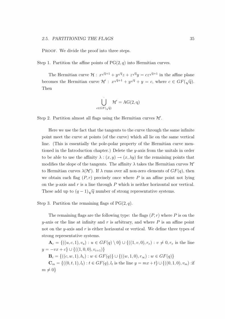
Proof. We divide the proof into three steps.

Step 1. Partition the affine points of PG(2, q) into Hermitian curves.

The Hermitian curve H : x√

q+1 + y√

qz + z√

qy = cz√

q+1 in the affine planebecomes the Hermitian curve H′ : x

√q+1 + y

√q + y = c, where c ∈ GF (

√q).

Then

.⋃c∈GF (

√q)

H′ = AG(2, q)

Step 2. Partition almost all flags using the Hermitian curves H′.

Here we use the fact that the tangents to the curve through the same infinitepoint meet the curve at points (of the curve) which all lie on the same verticalline. (This is essentially the pole-polar property of the Hermitian curve men-tioned in the Introduction chapter.) Delete the y-axis from the unitals in orderto be able to use the affinity λ : (x, y) → (x, λy) for the remaining points thatmodifies the slope of the tangents. The affinity λ takes the Hermitian curves H′

to Hermitian curves λ(H′). If λ runs over all non-zero elements of GF (q), thenwe obtain each flag (P, r) precisely once where P is an affine point not lyingon the y-axis and r is a line through P which is neither horizontal nor vertical.These add up to (q − 1)

√q number of strong representative systems.

Step 3. Partition the remaining flags of PG(2, q).

The remaining flags are the following type: the flags (P, r) where P is on they-axis or the line at infinity and r is arbitrary, and where P is an affine pointnot on the y-axis and r is either horizontal or vertical. We define three types ofstrong representative systems.

Ac = {((u, c, 1), vu) : u ∈ GF (q) \ 0} ∪ {((1, v, 0), rv) : v 6= 0, rv is the liney = −vx + c} ∪ {((1, 0, 0), vc+1)}

Bc = {((c, w, 1), hc) : w ∈ GF (q)} ∪ {((w, 1, 0), r∞) : w ∈ GF (q)}Cm = {((0, t, 1), lt) : t ∈ GF (q), lt is the line y = mx + t}∪ {((0, 1, 0), vm) :if

m 6= 0}


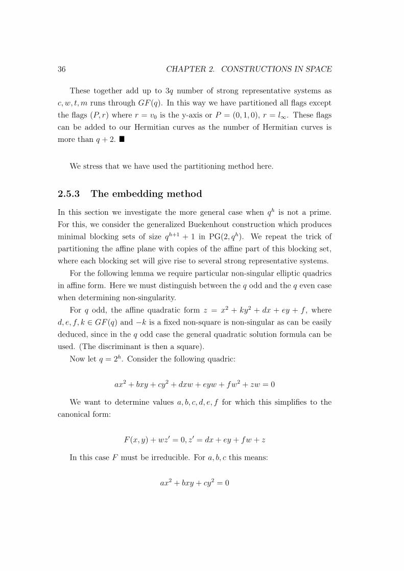
These together add up to 3q number of strong representative systems asc, w, t, m runs through GF (q). In this way we have partitioned all flags exceptthe flags (P, r) where r = v0 is the y-axis or P = (0, 1, 0), r = l∞. These flagscan be added to our Hermitian curves as the number of Hermitian curves ismore than q + 2.

We stress that we have used the partitioning method here.

2.5.3 The embedding method

In this section we investigate the more general case when qh is not a prime.For this, we consider the generalized Buekenhout construction which producesminimal blocking sets of size qh+1 + 1 in PG(2, qh). We repeat the trick ofpartitioning the affine plane with copies of the affine part of this blocking set,where each blocking set will give rise to several strong representative systems.

For the following lemma we require particular non-singular elliptic quadricsin affine form. Here we must distinguish between the q odd and the q even casewhen determining non-singularity.

For q odd, the affine quadratic form z = x2 + ky2 + dx + ey + f , whered, e, f, k ∈ GF (q) and −k is a fixed non-square is non-singular as can be easilydeduced, since in the q odd case the general quadratic solution formula can beused. (The discriminant is then a square).

Now let q = 2h. Consider the following quadric:

ax2 + bxy + cy2 + dxw + eyw + fw2 + zw = 0

We want to determine values a, b, c, d, e, f for which this simplifies to thecanonical form:

F (x, y) + wz′ = 0, z′ = dx + ey + fw + z

In this case F must be irreducible. For a, b, c this means:

ax2 + bxy + cy2 = 0


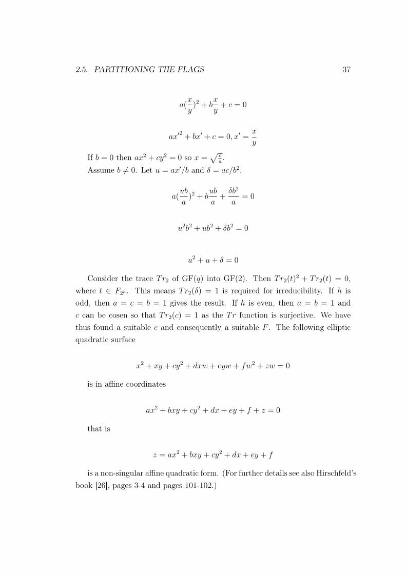
a(x

y)2 + b

x

y+ c = 0

ax′2+ bx′ + c = 0, x′ =

x

y

If b = 0 then ax2 + cy2 = 0 so x =√

ca.

Assume b 6= 0. Let u = ax′/b and δ = ac/b2.

a(ub

a)2 + b

ub

a+

δb2

a= 0

u2b2 + ub2 + δb2 = 0

u2 + u + δ = 0

Consider the trace Tr2 of GF(q) into GF(2). Then Tr2(t)2 + Tr2(t) = 0,

where t ∈ F2h . This means Tr2(δ) = 1 is required for irreducibility. If h isodd, then a = c = b = 1 gives the result. If h is even, then a = b = 1 andc can be cosen so that Tr2(c) = 1 as the Tr function is surjective. We havethus found a suitable c and consequently a suitable F . The following ellipticquadratic surface

x2 + xy + cy2 + dxw + eyw + fw2 + zw = 0

is in affine coordinates

ax2 + bxy + cy2 + dx + ey + f + z = 0

that is

z = ax2 + bxy + cy2 + dx + ey + f

is a non-singular affine quadratic form. (For further details see also Hirschfeld’sbook [26], pages 3-4 and pages 101-102.)


Lemma 2.21 Let F (X, Y ) denote a homogeneous irreducible quadratic polyno-mial over GF(q) and consider the following affine equation:

Z = F (X, Y ) + aX + bY + c.

As a, b and c run through all elements of GF(q), we find q3 elliptic quadrics withthe following properties:

(i) (0, 0, 1, 0) is the unique infinite point of all the quadrics;

(ii) every affine point is on q2 quadrics;

(iii) for any incident (P, α) pair with P an affine point and α a plane notthrough (0, 0, 1, 0), there is exactly one quadric through P for which α isa tangent plane (at P ).

Proof. It is easy to check that the q3 elliptic quadrics have (0, 0, 1, 0) as theonly point at infinity. (See [26], pages 101-102 for the fact that these are ellipticquadrics).

For (ii) note that after fixing x, y and z, the number of solutions for z−xa−yb− F (x, y) = c, is q2.

For (iii) recall that the tangent plane of the quadric Z = F (X, Y ) + aX +

bY + c at the point (x, y, z, 1) is the plane through the point and orthogonal tothe vector (F ′

X(x, y) + a, F ′Y (x, y) + b,−1, a + b + 2c− z) (see [26]). It is easy to

see that for fixed x, y and z this vector uniquely determines a, b and c. As allquadrics contain (0, 0, 1, 0), no tangent plane in question can pass through thispoint.

Lemma 2.22 Suppose that in the generalized Buekenhout construction we fixeverything apart from O and let O run through all ovoids from Lemma 2.21 withT corresponding to the point (0, 0, 1, 0). Then we find q3 minimal blocking setsof PG(2, qh) with the same unique infinite point that cover q2 times the affinepoints of M .


Proof. As 〈π, V 〉 = M , and π \ H was covered q2 times this is also true forthe affine part of M . (Any point in 〈P, V 〉, P ∈ π \H, is covered as many timesas P .)

Lemma 2.23 Pick two minimal blocking sets from Lemma 2.22 sharing thepoint P ∈ M \ H. Then the tangents to P will meet the line at infinity indisjoint pointsets (both of size qh−2) for the two cases.

Proof. 〈V, P 〉 meets π in a point P ′, this should be a common point of O1 andO2, the two ovoid bases for the two minimal blocking sets. From Lemma 2.21we know that the tangent planes α1 and α2 at P ′ have to be different. On theother hand, by Lemma 2.12 (iii), an h-space corresponding to a common tangentthrough P would meet M in a plane (disjoint from V ) within 〈α1, V 〉∩〈α2, V 〉 =

〈α1 ∩ α2, V 〉. This is not possible by dimensions.

Corollary 2.24 Let U denote the points of PG(2, qh) (considered in the André,Bruck-Bose representation) corresponding to the affine points of an (h + 2)-dimensional subspace M . Then one can partition all incident (point,line) pairswith the points chosen from U and lines not through a fixed infinite point Y ,into qh+1 strong representative systems.

Proof. Take the q3 minimal blocking sets considered in Lemma 2.22. Eachof them gives rise to qh−2 strong representative systems as follows. Using thenotations of Remark 2.14 (after fixing a blocking set) choose an infinite pointfrom each of the Ii-s and consider all tangents (and points of tangencies) througheach of them. This is a strong representative system of size qh+1. Let the chosenpoints run through all points of the corresponding Ii-s simultaneously to findqh−2 strong representative systems. Finally, repeat this for all q3 blocking sets.

By Lemmas 2.22 and 2.23 every point of U will occur in q2 blocking sets andall tangents will be different, hence a point is in q2 · qh−2 = qh flags, this is thenumber of lines through the point (except for the one joining the point to Y ).The number of strong representative systems used is q3 · qh−2 = qh+1.


Theorem 2.25 (Mengyán, [3]) The flags of PG(2, qh), h ≥ 2, can be parti-tioned into q2h−1 + 2qh strong representative systems.

Proof. Denote by H the hyperplane at infinity of PG(2h, q) and partition theaffine part with (h+2)-dimensional subspaces through a fixed (h+1)-dimensionalsubspace within H. This (through the André, Bruck-Bose representation) givesrise to a partitioning of the affine part of AG(2, qh) into qh−2 sets correspondingto affine parts of (h + 2)-spaces like in Corollary 2.24. Taking strong represen-tative systems guaranteed by the corollary, we find a partition of almost all theflags of the affine plane (into qh+1qh−2 = q2h−1 strong representative systems)except for one parallel class of lines. Hence to finish the proof we have to addstrong representative systems partitioning the uncovered flags as in the secondpart of Lemma 2.18 giving an additional 2qh strong representative systems.

In graph theoretic terminology we can thus answer the original question ofGyárfás [21] on the strong chromatic index of the point-line incidence graphof PG(2, q), for q not a prime. For this we recall that a strong colour classin a graph G is a set of independent edges with the extra property that thisset of edges is an induced subgraph of G, i.e. there are no edges in G joiningtwo end-points of different edges in this strong colour class. Consider now thepoint-line incidence graph G of PG(2, q) (that is, the points and lines are thetwo colorclasses and the edges are the flags of PG(2, q)). In G a strong colourclass is a strong representative system. The strong chromatic index of a graph G

is the minimum number of colours in an edge-colouring with the property thatthe edges having the same colour form a strong colour class. Geometrically, forG this chromatic index is the minimum number of strong representative systemscovering the flags of PG(2, q), the very question we have set out to solve.

Corollary 2.26 The strong chromatic index of the bipartite graph correspond-ing to PG(2, qh), qh a non-prime, is at most q2h−1 + 2qh.

We note that when q is prime no methods are presently known that are betterthan the trivial estimate. This is connected to the limit of the application ofthe embedding method to the non-prime case, and lack of knowledge of largeminimal blocking sets partitioning the affine plane (space).

Chapter 3

Constructions in the plane

In this chapter we will use constructional methods to answer a question origi-nally asked by György Turán whether the number of minimal blocking sets of agiven size is more than polynomial. The term more than polynomial1 refers toa function that grows faster than any polynomial of the variable, i.e. a functionof the form f(q) = qg(q), where limq→∞ g(q) = ∞.

3.1 Random constructions in the plane

3.1.1 The parabola construction

The arguments here are based on a paper by Szőnyi [43], where the author provesthe existence of a minimal blocking set of size between cq log q and Cq log q. Theidea of all constructions of the paper was to take the union of parabolas andeither prove that they form a minimal blocking set, or add some extra pointsto make the set a blocking set and consider the minimal blocking set inside theconstructed set. First we summarize some easy observations from [43].

Lemma 3.1 Let q ≡ 1(4) and T ⊆ GF(q). Set B = {(x, x2 + a, 1) : x ∈GF(q), a ∈ T} ∪ (0, 1, 0). Then the following hold:

• (i) There is a tangent through every point of B if and only if the differenceof any two elements in T is a non-square of GF(q);

1Some authors call this superpolynomial.

41

42 CHAPTER 3. CONSTRUCTIONS IN THE PLANE

• (ii) B is a blocking set if and only if for any s ∈ GF(q)\T there is a t ∈ T

such that t− s is a square in GF(q);

• (iii) for an s ∈ GF(q) \ T the points of the parabola {(x, x2 + s, 1) : x ∈GF(q)} are either all on at least one tangent to B or none of them is onany tangent;

• (iv) the point (a, b, 1) is on a tangent of B if and only if there is a t ∈ T

such that t− b + a2 is a square in GF(q).

Hence taking T to be maximal with respect to the property that the differ-ence of any two elements of T is a non-square, we find a minimal blocking set.It is difficult to determine the size of such a T . For a lower bound one has touse Theorem 1.13.

Applying this theorem it is easy to see that if |T | < c1 log2 q (where c1 < 12

and q is large enough), then one can find an s ∈ GF(q) such that s − t is anon-square for every t ∈ T , hence to make B become a blocking set B, we need|B| = 1 + q |T | ≥ 1 + c1q log2 q. The problem is that we cannot give an upperbound on the size of B, for instance if q is a square, then T can be taken to bea multiplicative coset of the subfield GF(

√q) giving a minimal blocking set of

size q√

q + 1. The trick sketched in Szőnyi’s paper is to let |T | = c1 log2 q (for afixed c1 < 1

2) and try to add points (but hopefully not whole parabolas) to B to

complete it to a minimal blocking set. The following lemma from [22] handlesa very general setting for random choice, which could be used here.

Lemma 3.2 Let G be a bipartite graph with bipartition L ∪ U . Suppose thatthe degree of vertices in U is at least d. Then there is a set L

′ ⊆ L, |L′| ≤|L|(1 + log |U |))/d, such that any u ∈ U is adjacent to a vertex of L

′.

To complete B to a blocking set B′, we have to add points blocking all linesnot blocked by B. These will be found by using Lemma 3.2. We will not beable to guarantee that the resulting blocking set is minimal, all we can do is toassure that the points of B will still have their tangents (this will then guaranteethat the minimal blocking set contained in the constructed blocking set is of

3.1. RANDOM CONSTRUCTIONS IN THE PLANE 43

size at least |B|). For this, we will only choose from those points, which are onno tangents of B.

Let the vertex class U (of a bipartite graph) correspond to the lines notblocked by B and the vertex class L correspond to points of PG(2, q) which lieon no tangents of B. Draw an edge between a point of U and a point of L ifthey correspond to an incident (point,line) pair. To use Lemma 3.2, we have tobound |U |, |L| and the minimum degree d in U .

For an upper bound on U , one can simply take |U | ≤ q2.For an upper bound on L, note that by Lemma 3.1 (iii), |L| = ql, where l

is the number of elements s ∈ GF(q) \ T such that s− t is a non-square for allt ∈ T . By Theorem 1.13 l ≤ q

2|T | +√

q+1

2|T | < 2q1−c1 .

To find a lower bound on d, consider a line X1 = mX0 + bX2 not blockedby B. By Lemma 3.1 (iv) we have to count the number of points (x, mx + b, 1)

such that t− (mx + b) + x2 is a non-square for all t ∈ T . Using Theorem 1.13(for the polynomials t − (mx + b) + x2) we have that this number is at least

q2|T | − (

√q + 1) |T | ≥ 1

2q1−c1 for large enough q.

Applying Lemma 3.2 gives that we need to add at most |L| 1+log|U |d

≤ c2q log q

points to B to find a blocking set B′ (note that here we have log q, while forthe size of B we had log2 q, but these two are constant multiples of each other).This will have the property that through points of B we have tangents, hencethe size of the minimal blocking set inside B′ is between c1q log2 q = cq log q andc1q log2 +c2q log q = Cq log q.

Theorem 3.3 (Mengyán, [2]) There are constants c and C such that for q ≡ 1

(mod 4), the number of non-isomorphic minimal blocking sets in PG(2, q) ofsize from the interval [cq log q, Cq log q] is more than polynomial.

Proof. First we count the number of ways one can choose the set T . Thefirst point of T can be arbitrary, the number of choices for the second oneis exactly q−1

2,..., for the last point, by Theorem 1.13, we still have at least

q2|T |−1 −

√q+1

2(|T | − 1) ≥ q1−c1 choices. Hence the number of ways to choose T is

at least (q1−c1)|T |. In a resulting minimal blocking set there are at most C log q

parabolas, hence at most(

C log q|T |

)< (C log q)|T | different T -s can give the same

minimal blocking set. Thus all in all we have constructed at least


(q1−c1

C log q)|T |

minimal blocking sets, this is more than polynomial.

A similar argument (also based on a construction sketched in Szőnyi’s paper)works for the case q ≡ 3 (mod 4) showing that again there are more thanpolynomial minimal blocking sets of size approximately cq log q. In this caseapproximately half of the points from the considered parabolas (here againTheorem 1.13 determines the parabolas) are included in the minimal blockingset.

3.1.2 Blocking sets arising from a Hermitian curve

It is easy to see that the properties of a Hermitian curve H (described in theIntroduction) imply that if we delete all but one points from a (

√q + 1)-secant

of H and add the pole of this line, then we find a minimal blocking set √q − 1

smaller than H. This is the adding and deleting points method. Throughoutthe section we try to iterate this procedure.

Construction 3.4 Given a Hermitian curve H consider a point P ∈ H and itstangent t. Choose lines l1, ..., li through P different from t. Delete all points of Hon these lines except for P and add to the set the poles l⊥1 , ..., l⊥i ∈ t. If i ≤ √q,then the resulting set is a minimal blocking set of size q

√q + 1− i(

√q − 1).

Theorem 3.5 (Mengyán, [2]) There are more than polynomial minimal block-ing sets in PG(2, q), q square, of size q

√q+1− i(

√q−1), where log q < i ≤ √q.

Proof. In Construction 3.4 we have more than(

qlog q

)choices for the deleted

secants. This is more than polynomial.

Construction 3.4 works only for i ≤ √q; for i ≥ √

q + 1 we might delete allpoints of a √q + 1 secant (not through P ). This means that the adding anddeleting method is insufficient by itself, and the trivial random method must beapplied.

3.1. RANDOM CONSTRUCTIONS IN THE PLANE 45

In what follows we restate and use results from [4], where the above men-tioned problem is handled. First we restate Theorem 4.2 from that paper.

Theorem 3.6 (Szőnyi, Cossidente, Gács, Mengyán, Siciliano, Weiner, [4])For an arbitrary square prime power q there is a minimal blocking set in PG(2, q)

for any size in the interval [4q log q, q√

q − q + 2√

q].

Now we follow the proof of this theorem with some necessary modifications.

Lemma 3.7 Let P be a point of a Hermitian curve H, m a (√

q + 1)-secantnot through P . Then there exists a set A of secants through P of size at most3√

q log q + 1 with the following properties:

(1) all but one secant in A meet m in a point outside H;

(2) the points of H on secants in A block all secants to H not through P .

Proof. We use Lemma 3.2. Choose a line l1 through P meeting m in a pointof the curve. Let the vertices in L correspond to secants through P meetingm in a point outside the curve and the vertices in U correspond to secants notthrough P not blocked by points of H on l1. Draw an edge between a vertex ofU and a vertex of L if and only if the corresponding lines meet in a point of H.We have |L| = q −√q − 1, |U | ≤ q2.

Next we prove that the minimum degree in U is at least √q− 1. For this werecall that as H is classical all secants to H meet H in a Baer subline. If thedegree of some vertex in U was less than √q− 1, then this would correspond toa secant m

′ 6= m not through P that meets at most √q−2 secants (correspond-ing to vertices of L) in a point outside the curve. Consider the √q + 1 linesl1, ..., l√q+1 of P meeting m inside H. Since the degree of m

′ is at most √q− 2,m

′ must meet at least three of these lines in a point of H. Using the fact thatthe points of H ∩ m′ form a Baer subline and that three points (respectivelylines) uniquely determine a Baer subline (respectively Baer pencil), we deducethat the points in m

′ ∩H are exactly the points li ∩m′ (i = 1, ...,

√q + 1). But

then l1 blocks m′ contrary to the assumption, so we deduce d ≥ √

q − 1. Aneasy calculation shows that Lemma 3.2 guarantees the existence of the set A.


Construction 3.8 Let H be a Hermitian curve, P ∈ H, t the tangent throughP . Let m be a secant not through P . Let l1 be a line through P meeting m ina point of H. Partition all the non-tangent lines through P to sets A,B,C,D,Ewith the following properties:

(1) Let A be a set coming from Lemma 3.7, l1 ∈ A. Add to A the polar lineof m ∩ t. Hence |A| ≤ 3

√q log q + 2;

(2) B ∪ C are the lines through P (besides l1) meeting m in a point of H.

Delete the point l ∩m for all l ∈ B and delete all points of H from the linesof C and D, except for P . Add to the set poles of deleted lines. Finally, addthe pole of m.

This results in a set of size q√

q + 2− |B| − |C ∪D|(√q − 1).

Lemma 3.9 The set given in Construction 3.8 is a minimal blocking set.

Proof. With the introduced notation A blocks all secants not through P ,secants through P are blocked by P and the added points block the tangents ofdeleted points. Remaining points of H have their original tangents except forl1 ∩m that has m as tangent and for P that has tangents from C ∪D. Finally,the added points have the tangents of deleted points.

Theorem 3.10 (Mengyán, [2]) In PG(2, q) there are more than polynomialnon-isomorphic minimal blocking sets for any size in the interval

[5q log q, q

√q − 2q

]whenever q is a square.

Proof. For a minimal blocking set of size k ∈ [5q log q, q√

q − 2q] write k =

q√

q + 2 − R(√

q − 1) − Q with 0 ≤ Q ≤ √q − 2. An easy calculation shows

that here q − 5√

q log q +√

q ≥ R ≥ 2√

q + 1. If we use Construction 3.8 with|B| = Q and |C ∪D| = R, the resulting blocking set is of size k. After choosingB and C, D can be chosen in

(q−(

√q+1)−|A|+1

|D|

)>

(q−4

√q log q

|D|

)ways. The bounds

for R imply √q + 1 ≤ |D| ≤ q − 5√

q log q +√

q, hence the binomial coefficientis more than polynomial in q.

3.2. THE METHOD OF SUBSETS AND COSETS 47

3.2 The method of subsets and cosets

3.2.1 Blocking sets from a triangle

In this part we will use subsets. Originally, this involved the addition and dele-tion method, where one could determine the properties of the deleted points forcertain added points. These observations were then described in the terminol-ogy of subsets. In essence (with the terminology mentioned in the first chapter)we place subsets (the added points) on lines and delete some subsets from otherlines. The conditions on the added subsets ensure that these structures are min-imal blocking sets. Moreover, as we add two subsets H and K for this purpose;one is used to control the size of the minimal blockig set as required, the othergives the more than polynomial choices.

Below we prove the following theorem.

Theorem 3.11 (Mengyán, [2]) In PG(2, q) there are more than polynomialnon-isomorphic minimal blocking sets for any size in the interval [2q − 1, 3q − 4]

whenever q is odd or q is even and q − 1 is not a prime.

For this purpose we construct minimal blocking sets of size between 2q − 1

and 3q − 4 using particular subsets. All constructions can be considered asgeneralizations of the IMI construction originally due to Innamorati, Maturo[28] and Illés, Szőnyi, Wettl [27]. This and all the generalizations start from thefollowing minimal blocking set:

4 = {(x, 0, 1) : x 6= 0} ∪ {(0, y, 1) : y 6= 0} ∪ {(1, y, 0) : y 6= 0}.

Hence we take three sides of a triangle with the vertices removed2.First we recall the original construction.

Construction 3.12 (IMI) Choose a set K ⊂ GF(q)\{0} such that 1,−1 ∈ K.The set

IK = 4∪ {(1, y, 1) : y ∈ K} \ ({(1, y, 0) : y ∈ K} ∪ {(0, y, 1) : y ∈ K})2This is also called the vertexless triangle.


is a minimal blocking set of size 3q − 3− |K|.

The IMI construction gives minimal blocking sets for each value in the inter-val [2q− 1, 3q− 4]. It is easy to see, that whenever K has to have size between√

q and q−√q, then the number of choices is more than polynomial. Hence theconstruction automatically gives the following.

Theorem 3.13 There are more than polynomial minimal blocking sets for anysize in the interval [2q +

√q, 3q −√q].

However, for the intervals [3q −√q, 3q − 4] and [2q − 1, 2q +√

q] we will haveto generalize the IMI construction in two different ways.

Construction 3.14 Suppose K, H ⊂ GF(q) \ {0} satisfy the following condi-tions:

(1) −H = H;

(2) (1−H) ∩K = ∅;

(3) K ∩H = {1}.

Then

4∪ {(x, x, 1) : x ∈ H} ∪ {(1, y, 1) : y ∈ K} \

({(1, y, 0) : y ∈ K} ∪ {(0, y, 1) : y ∈ K ∪H})

is a minimal blocking set of size 3q − 3− |K|.

Proof. It is straightforward to check that the constructed set blocks every line:all lines are blocked by the points of the line X0 = 0, except for those through(0, 0, 1) or (1, 0, 0). The line X1 = yX0 through (0, 0, 1) is blocked by either thepoint (1, y, 1) or (1, y, 0) according to whether y ∈ K or not. Similarly the lineX1 = yX2 through (1, 0, 0) is blocked by either the point (0, y, 1) or (1, y, 1) or(y, y, 1) according to whether y /∈ H ∪K or y ∈ K or y ∈ H.

For the minimality note that for a point of the form (1, y, 1) with y ∈ K or(y, y, 1) with y ∈ H or (0, y, 1) with y /∈ H ∪K, the line X1 = yX2 is a tangent.


Through a point of the form (1, y, 0), y /∈ K, the line X1 = yX0 is a tangent.Similarly, for a point of the form (x, 0, 1) with x /∈ H, the line X0 = xX2 isa tangent. The only non-trivial part is to check, whether one has a tangentthrough a point of the form (x, 0, 1), x ∈ H. A little calculation shows that forsuch a point, the line X1 = X0 − xX2 is a tangent.

Theorem 3.15 There are more than polynomial minimal blocking sets for anysize in the interval [3q −√q, 3q − 4].

Proof. To achieve the size k ∈ [3q−√q, 3q−4], choose a set K from GF(q)\{0}with |K| = 3q − 3 − k and 1 ∈ K, −1 /∈ K. Apply Construction 3.14 with anappropriate H of size √q. The number of choices for such an H is at least((q−3−4

√q)/2

(√

q−2)/2

), which is more than polynomial (note that the only elements we

cannot use for H are those from K ∪ (1−K) ∪ (−K) ∪ (K − 1)).

The following construction works for the q odd case, as then −2 6= 2.

Construction 3.16 Let the order of the plane be odd.Suppose K, H ⊂ GF(q) \ {0} satisfy the following conditions:

(1) H ∩K = ∅

(2) 2 ∈ H, −2 ∈ K;

(3) 1 ∈ K;

(4) (K \ {−2}) = −(K \ {−2})

Then

4∪ {(1, y, 1) : y ∈ K} ∪ {(−1, y, 1) : y ∈ H} \

({(1, y, 0) : y ∈ (−H) ∪K} ∪ {(0, y, 1) : y ∈ H ∪K})

is a minimal blocking set of size 3q − 2− |H| − |K|.


Proof. The proof is almost identical to the proof of Construction 3.14. Itis straightforward to check that the constructed set blocks every line: all linesare blocked by the points of the line X0 = 0, except for those through (0, 0, 1)

or (1, 0, 0). The line X1 = yX0 through (0, 0, 1) is blocked by either the point(1, y, 0) or (1, y, 1) or (−1, y, 1) according to whether y /∈ H ∪ K or y ∈ K ory ∈ H. Similarly the line X1 = yX2 through (1, 0, 0) is blocked by either thepoint (0, y, 1) or (1, y, 1) or (−1, y, 1) according to whether y /∈ H ∪K or y ∈ K

or y ∈ H.For the minimality note that for a point of the form (1, y, 1) with y ∈ K

or (−1, y, 1) with y ∈ H or (0, y, 1) with y /∈ H ∪ K, the line X1 = yX2 is atangent. Through a point of the form (1, y, 0), y /∈ H ∪K, the line X1 = yX0 isa tangent. Similarly, for a point of the form (x, 0, 1) with x /∈ {−1, 1}, the lineX0 = xX2 is a tangent. The only non-trivial part is to check, whether one hasa tangent through the points (−1, 0, 1) and (1, 0, 1). A little calculation showsthat at (−1, 0, 1) the line through (0,−2, 1) is a tangent and at (1, 0, 1) the linethrough (0, 1, 1) is a tangent.

Theorem 3.17 There are more than polynomial minimal blocking sets for anysize in the interval [2q − 1, 3q − 3− q−1

2].

Proof. For a k ∈ [2q−1, 3q−3− q−12

] one should choose K such that |K| = q−12

and then H with |H| = 3q − 2− q−12− k in Construction 3.16. The number of

choices for K is roughly(

q/2q/4

).

Putting together Theorems 3.12, 3.15 and 3.17, we obtain Theorem 3.11,except for the even case. (And note that even for the 2|q case the only partof [2q − 1, 3q − 4] where we have not been able to show more than polynomialminimal blocking sets is [2q−1, 2q+

√q].) The following construction completes

the proof of Theorem 3.11, since if q − 1 is not a prime, we can always find anappropriate M .

Construction 3.18 For an even prime power q let M denote a multiplicativesubgroup of GF(q) with generator element t, with |M | = d, 3 ≤ d ≤ √q.


Suppose K,H ⊂ GF(q) \ {0} satisfy the following conditions:

(1) t ∈ H;

(2) t + 1 /∈ H, t+1t

/∈ K;

(3) H ∩K = ∅;

(4) 1tiH \ {t + 1} = H for i = 0, 1, ..., d− 1.

The set H is thus the union of cosets of M , except possibly for the elementt + 1.

The set

4∪ {(1, y, 1) : y ∈ K} ∪ {(t, y, 1) : y ∈ H} \

({(1, y, 0) : y ∈ H ∪K} ∪ {(0, y, 1) : y ∈ H ∪K})

is a minimal blocking set.

The size of the blocking set is 3q − 3 − |H| − |K|, and since 3 ≤ d ≤ √q,

we have more than polynomial choices for a suitable H. For instance, let |H| =[ q−1

2d] · d and |K| ≤ q− 3− |H|. To get a particular minimal blocking set of size

k (from Construction 3.18) first choose H then choose K; as the size of H isfixed the size of K will determine k. That is k = 3q − 3− [ q−1

2d] · d− |K|. The

number of choices is(

(q−1)/d−1[(q−1)/2d]−1

)(q−3−|H|

3q−3−|H|−k

), i.e. more than polynomial.

For the constructions above we have used certain “good” subsets, but thelast construction “almost” employed cosets, which takes us to the theme of theremaining part of the present thesis.

3.2.2 Megyesi’s construction

Megyesi’s construction is the following Rédei construction using cosets.

Construction 3.19 (Megyesi) Let H be a non-trivial multiplicative subgroupof (GF(q), ·). Partition (GF(q), ·) into two nonempty subsets X and Y in sucha way that both are the union of cosets of H. Let U = {(x, 0) : x ∈ X}∪{(0, y) :

y ∈ Y } ∪ {(0, 0)}. Finally, let D denote the determined directions of U . ThenU ∪D is a minimal blocking set.


The following lemma will determine the size of the minimal blocking set inConstruction 3.19.

Lemma 3.20 The size of a minimal blocking set M using Construction 3.19 is2q + 1− |K|, where K = {k : k ·X = X}.

Proof. We wish to prove that the non-determined directions are exactly thosecorresponding to elements of −K. A direction (d) /∈ {(0), (∞)} is determinedif and only if d = −y

xfor suitable x ∈ X and y ∈ Y . This is equivalent to the

condition −dX ∩ Y 6= ∅ ⇔ −dX 6= X ⇔ d /∈ −K.

Note that K is the largest multiplicative subgroup for which X (and Y ) isthe union of some cosets of K and H ⊆ K. Hence instead of starting with H,we can start with K and the same X and Y to get the same blocking set.

Lemma 3.21 Given a multiplicative subgroup H of (GF(q), ·) with index h > 3,the number of ways of choosing X and Y in Construction 3.19 to have size2q + 1− |H| is greater than 2h−1.

Proof. There are 2h−2 choices for X and Y . The number of choices for whichthe number of non-determined directions is |K| for a larger group than H is atmost

∑(2h′ − 2), where the summation is over all h′|h, h′ 6= h, h′ 6= 1. This is

at most 2 + 4 + · · ·+ 2h/2 − 2 = 2h/2+1 − 4.

Theorem 3.22 (Mengyán, [2]) Let d be an arbitrary integer, 2 ≤ d ≤ √q,

d|q− 1. The number of minimal blocking sets M of size 2q +1− d is more thanpolynomial.

Proof. Let H ≤ GF(q, ·), |H| = d. Then the index is h = q−1d≥ √q−1. From

Lemma 3.21 the number of choices for X and Y in construction 3.19 is greaterthan 2h−1.

There is a similar construction due to Megyesi with additive subgroups. Theonly exception is that one has to put some cosets of an (additive) subgroup on


a line and the rest to a parallel line. Using this, one can prove a similar resultfor blocking sets of size 2q + 1− d, where d|q, d ≤ √q.

We note that in PG(n, q) considering a cone with an (n − 3)-dimensionalsubspace as vertex V and with the minimal blocking sets constructed in thischapter as base B we get again minimal line-blocking pointsets, so equivalentstatements proved in the chapter exist in higher dimensions.

Chapter 4

A generalization of Megyesi’sconstruction

A different example than Megyesi’s construction, contained in the union offour lines, was constructed by Gács [23] giving an infinite series of examplesdetermining 7q/9 directions approximately, thus yielding a minimal blockingset of approximate size 2q − 2q/9.

Theorem 4.1 (Gács, [23]) Let 3 be a divisor of q − 1, and let 1, α, α2 be cosetrepresentatives of the multiplicative subgroup G of index 3. Let

Ui = {(0, 0)} ∪ {(x, 0) : x ∈ αiG} ∪ {(x, x) : x ∈ G} ∪ {(0, x) : x ∈ αiG}.

Denote by |Di| the number of directions determined by Ui. Then |D1| +

|D2|+ |D3| = 3q + 1− 2(q − 1)/3, and |Di| = 7q/9 + O(√

q).

In both the Megyesi and the Gács constructions a subgroup and its cosetswere placed on lines. The question arises whether a generalization would bepossible when the number of cosets is larger than three, or when the number oflines from which points are taken is increased. As we show in this chapter thisproblem can be formulated using some trivial equations and solved by Weil’sestimate.

In some sense the technique we use here is similar to techniques used byKorchmáros in [31] and Szőnyi in [42], though our method seems distinct fromtheirs.

55

56CHAPTER 4. A GENERALIZATION OF MEGYESI’S CONSTRUCTION

4.1 Placing cosets on three lines

In this section we investigate the case when the points of the minimal blockingset are on four lines: three concurrent lines in AG(2, q) and the fourth the lineat infinity of the projective closure of AG(2, q). In particular, without loss ofgenerality, we may assume the three affine lines to be x = 0, y = 0 and x = y.

Construction 4.2 Consider a multiplicative subgroup G of (GF(q), ·) with in-dex s, such that α is a generator element of G. Form three non-empty subsetsI, J, K from the set of integers S = {0, ..., s− 1} such that |I| + |J | + |K| = s.Let

U = {(0, 0)} ∪⋃j∈J

(0, αjG) ∪⋃k∈K

(αkG, αkG) ∪⋃i∈I

(αiG, 0).

Then the set B = U ∪D, where D is the set of directions determined by U

and |D| < q + 1, is a minimal blocking set.

Proof. Minimality follows from the fact that not all q + 1 directions can bedetermined.

The size of the minimal blocking set B of Construction 4.2 can be determinedby determining |D|. This is equivalent to determining |Dc|, the number of non-determined points, as |D| + |Dc| = q + 1. Note also that S is a multiplicativesubgroup, and that operations on S are considered modulo s.

Lemma 4.3 Consider a multiplicative subgroup G of (GF(q), ·) with index s,such that α is a generator element of G and a set of integers S = {0, ..., s− 1}.Then

.⋃u∈S

−αuG = GF(q) \ {0}

.⋃w∈S

1− αwG = GF(q) \ {1}

.⋃v∈S

11−αvG

= GF(q) \ {0, 1,∞}.

4.1. PLACING COSETS ON THREE LINES 57

Proposition 4.4 For B in Construction 4.2 we have:

1. D = {0, 1,∞} ∪ (⋃

u∈J−I

−αuG) ∪ (⋃

v∈I−K

11−αvG

) ∪ (⋃

w∈J−K

(1− αwG));

2. Dc = {0, 1,∞}c ∩ (⋃

u∈J−I

−αuG)c ∩ (⋃

v∈I−K

11−αvG

)c ∩ (⋃

w∈J−K

(1− αwG))c.

where c denotes the complement.

Proof. Considering the directions the cosets determine, one gets D. Anelement of Dc must come from the intersections of the complements, as otherwiseit would be determined.

Proposition 4.5 From Proposition 4.4 and Lemma 4.3 it follows that

Dc = (⋃

u 6∈J−I

−αuG) ∩ (⋃

v 6∈I−K

1

1− αvG) ∩ (

⋃w 6∈J−K

(1− αwG)).

Lemma 4.6 Consider a multiplicative subgroup G of (GF(q), ·) with index s,such that α is a generator element of G. Then

1. −αuG ∩ 11−αvG

∩ (1− αwG) = ∅ if u + v 6= w,

2. −αuG ∩ 11−αvG

= −αuG ∩ (1− αwG) = 11−αvG

∩ (1− αwG) if u + v = w,

for any u, v, w ∈ (GF(q), ·).

Proof. 1. For an element in the intersection 11−αvG

∩ (1 − αwG) we have1

1−αvx= (1 − αwy) for some x, y ∈ G. Then (1 − αwy)(1 − αvx) = 1, which

implies 1 − αwy = −αwyαvx

= −αw−v yx∈ −αw−vG. If u + v 6= w then αu 6= αw−v

so αuG and αw−vG are disjoint cosets.2. We essentially follow the proof of Lemma 3.4 of [23] showing that −αuG∩

(1− αwG) ⊂ −αuG ∩ 11−αvG

⊂ 11−αvG

∩ (1− αwG) ⊂ −αuG ∩ (1− αwG).The intersection −αuG ∩ (1− αwG), means that −αux = 1− αwy for some

x, y ∈ G. Dividing by −αux one gets 1 = −1αux

+ αwyαux

, implying −αux = 1

1−αwyαux

=

11−αv x

y∈ 1

1−αvG.


Next let −αux = 11−αvy

. Rearranging and using that u + v = w we get−αux = 1− αwy ∈ 1− αwG.

Finally, set 11−αvx

∩ (1 − αwy). Then 1 = (1 − αwy)(1 − αvx). Again afterrearranging we get 1− αwy = −αw−v y

x∈ −αuG.

Notation 4.7 Denote by the pair (u, w) the intersection −αuG ∩ (1− αwG).

Corollary 4.8 Dc is the sum of intersections of the form −αuG ∩ 11−αvG

∩(1 − αwG). By Lemma 4.6 1. only those intersections are non-empty whereu + v = w, and by Lemma 4.6 2. any of the three intersections determine thesame non-empty intersection, so it is enough to consider (u, w).

To determine the size of (u, w) for given u and w Weil’s estimate is used.

Lemma 4.9 The number of points in −αuG∩(1−αwG) is approximately q/s2+

O(√

q).

Proof. The elements of G are precisely the elements of the form us, where0 6= u ∈ GF(q). Hence the elements of −αuG ∩ (1 − αwG) correspond to thesolutions of the equation

axs = 1− bys, (4.1)

where a = αu and b = αw are nonzero elements of GF(q), and 0 6= x, y.Actually, for an element g of G there are s elements u ∈ GF(q) such thatg = us. Hence a common element of −αuG ∩ (1 − αwG) correspond to s2

solutions of equation (4.1). Furthermore, (4.1) defines an affine curve whoseprojectivization is axs = zs − bys (here (x, y, z) denotes the homogeneous coor-dinates). This projective curve has no singular points, since g.c.d.(s, q) = 1. ByWeil’s estimate, the number of GF(q)-rational points of the projective curve isq+1− (s−1)(s−2)

√q ≤ N ≤ q+1+(s−1)(s−2)

√q. The curve has s infinite

points, there are at most s points on any of the lines x = 0 and y = 0. Therefore(4.1) has at least q+1−(s−1)(s−2)

√q−3s, and at most q+1+(s−1)(s−2)

√q

points. Dividing by s2 gives that

| − αuG ∩ (1− αwG)| ≤ q

s2+

(s− 1)(s− 2)

s2

√q +

1

s2

4.1. PLACING COSETS ON THREE LINES 59

| − αuG ∩ (1− αwG)| ≥ q

s2+

(s− 1)(s− 2)

s2

√q − 3s− 1

s2

that is | − αuG ∩ (1− αwG)| is q/s2 + O(√

q).

Remark 4.10 Note that the result is meaningful only when q/s2 � √q, that is

when s � 4√

q.

To determine the number of nonempty (u, w) pairs the following lemma canbe useful.

Lemma 4.11 Let I, J, K be subsets of a set of integers S = {0, ..., s− 1} withu, v, w ∈ S. Then the following hold modulo s:

u 6∈ J − I =⇒ I + u ∩ J = ∅

v 6∈ I −K =⇒ K + v ∩ I = ∅

w 6∈ J −K =⇒ K + w ∩ J = ∅

If furthermore u+ v = w then these together are equivalent to I +u∩J = ∅,K + w ∩ I + u = ∅ and K + w ∩ J = ∅.

Determining Dc and D in Construction 4.2 reduces to determining |T |, thenumber of pairs (u, w) satisfying the three equations of Lemma 4.11 involvingI, J, K and u, w. Each (u, w) pair then adds approximately q/s2 to |Dc|, so|B| = 2q − |T |q/s2 + O(

√q).

In this way constructing a minimal blocking set B using cosets is equivalentto solving some trivial equations. The size of B depends on |T | and a certainremainder term O(

√q) (the remainder term in Weil’s estimate); and if q is large

enough then mainly on |T |. So if q is large enough and there is a non-empty set(u, w) then the method certainly gives minimal blocking sets of size less than2q−1. (Otherwise the remainder term may be too large). Hence these minimalblocking sets are in the third interval of the spectrum.

Using the correspondence between the described trivial equations and min-imal blocking sets, we can construct minimal blocking sets of many sizes.


Example 4.12 Let I = {0}, J = {2, 3, ..., s − 1} and K = {1}. Then wehave two pairs (0, 0) and (1, s − 1) that satisfy Lemma 4.11. That is |N | =

2q/s2 + O(√

q), |B| = 2q − 2q/s2 + O(√

q).

Example 4.13 Let I = {0, 2}, J = {1} and K = {3, 4, ..., s−1}. Then we haveexactly one pair (0, 0) that satisfies Lemma 4.11. That is |N | = q/s2 + O(

√q),

|B| = 2q − q/s2 + O(√

q).

Example 4.14 Let s = 8k, for some positive integer k, I = {0, 2, 4, ...}, J =

{1, 5, 9, ...} and K = {3, 7, 11, ...}. Then the number of pairs that satisfy Lemma4.11 is 8k2 giving |N | = (q + 1)/8 + O(

√q), |B| = 2q − (q + 1)/8 + O(

√q).

Example 4.15 Let s = 3k, for some positive integer k, I = {0, 3, 6, ...}, J =

{1, 4, 7, ...} and K = {2, 5, 8, ...}. Then the number of pairs that satisfy Lemma4.11 is 2k2 giving |N | = 2q/9 + O(

√q), |B| = 2q − 2q/9 + O(

√q).

A thorough generalization of the Megyesi construction was done by NóraViola Harrach in [1], where she investigated the general case (cosets on morethan three lines), and gave a more abstract description that allows a completecharacterization of minimal blocking sets obtainable from cosets on lines. Forher results Sziklai’s version of the Weil estimate is needed (Theorem 1.14).

4.2 Embedding and non-Rédei minimal blocking

sets

From the existing minimal blocking sets some new ones can be constructed byusing embeddings of PG(2, q) into PG(2, qh) for some h > 1. In this section weinvestigate two possible methods mainly with recpect to the minimal blockingsets constructed above.

Construction 4.16 Consider a minimal blocking set B of PG(2, q). EmbedPG(2, q) into PG(2, qh) for some h > 1. Denote by l and m two lines ofPG(2, qh) that intersect PG(2, q) in q + 1 points, and B in less than q points

4.2. EMBEDDING AND NON-RÉDEI MINIMAL BLOCKING SETS 61

if Q := l ∩m is not a point of B. Furthermore denote by C the set of criticalpoints of B which have their critical tangents through Q. Consider the pointset

B′ = B ∪ {l \ PG(2, q)} ∪ {m \ PG(2, q)} ∪ {Q} \ C.

We note that if B is of size less than 2q then all lines intersect B in at mostq−1 points, for otherwise through any point of B on the existing q-secant thereare q lines that must be blocked, consequently the size of B would be at least2q.

Proposition 4.17 B′ in Construction 4.16 is a minimal blocking set in PG(2, qh)

of size

1. 2qh − 2q + |B| if Q ∈ B,

2. 2qh − 2q + |B|+ 1 if Q 6∈ B and C is empty.

Proof. Observe that any line of PG(2, qh) through a point of l ∩ PG(2, q) isblocked by the points of B, m or the point Q, and the points of B′ on l\PG(2, q)

block the remaining lines proving the blocking property.Minimality follows as at all points of B′ there are tangents. At the points

of B the lines containing the tangents to B in PG(2, q) are tangents as theseintersect l and m in l ∩ PG(2, q) and m ∩ PG(2, q) respectively. At the pointsof B′ on l \ PG(2, q) the lines through the points of {m ∩ PG(2, q) \ B} aretangents, and at the points of B′ on m \ PG(2, q) the lines through the pointsof {l ∩ PG(2, q) \ B} are tangents. At Q all the lines of PG(2, qh) intersectingPG(2, q) in exactly Q are tangents to B′.

The size of B′ is simply |l \ PG(2, q)| + |m \ PG(2, q)| + |B| if Q ∈ B andone more if Q 6∈ B.

The size of B′ when |C| > 1 and Q 6∈ B depends on B as some points of C

must be deleted, so the precise size can be only determined given the concretecase.

Proposition 4.18 Let x > 1 be an integer. If the size of B is 2q − x then thenumber of tangents at any point of B is at least x + 1, so there are no criticalpoints of B.


Proof. We follow the argument of Blokhuis and Brouwer from [12] that isbased on a result of Jamison [30]. If B is a minimal blocking set then eachpoint of B is on at least one tangent. Let P ∈ B be a point on t tangents, callone of them l. Form a blocking set of AG(2, q) = PG(2, q)\l with |B|−1+(t−1)

points by placing a point on each of the t − 1 tangents (6= l) of P and takingthe points of B \ {P}. Then the inequality t ≥ 2q + 1 − |B| can be deduced,because in [14] Brouwer and Schrijver proved that a blocking set of AG(2, q)

has at least 2q − 1 points.

Theorem 4.19 (Harrach and Mengyán, [1]) Let x > 1 be an integer. If there isa minimal blocking set of size 2q−x in PG(2, q) then there are minimal blockingsets of size 2qh − x and 2qh − x + 1 in PG(2, qh).

Note that for the minimal blocking sets of size 2q − x (x > 1) constructedpreviously in this chapter the number of tangents at affine points is |Dc| = x+1

and at infinite points at least q/s ≥ x + 1. When B is such a minimal blockingset then B′ of Construction 4.16 is a Rédei minimal blocking set if and only ifl∩PG(2, q) or m∩PG(2, q) are Rédei lines of B. For this, it is enough to checkthe sizes of the intersection of lines with B′ in PG(2, qh). For B′ to be Rédeithis intersection size must be qh− x for some line. But this is impossible as thesizes of possible intersections are at most q + 1 for the lines other than l or m.

Example 4.20 In Example 4.12 let l be the x-axis and m be the line y = x.Then the embedding of this minimal blocking set with the method above will bea non-Rédei minimal blocking set.

We now turn attention to another embedding method, described in [37] and[45]. Here we only repeat the construction and a theorem from these papers, andinvestigate what this method means for the minimal blocking sets obtained inthis chapter. For further details of this construction refer to the papers [37, 45].

Construction 4.21 Let B be a minimal blocking set in PG(2, q). Embed PG(2, q)

into PG(h+1, q). Choose an (h−2)-dimensional subspace V ′, so that PG(2, q)∩V ′ = ∅. Let B′ be the cone with base B and vertex V ′. Embed PG(h + 1, q)

4.2. EMBEDDING AND NON-RÉDEI MINIMAL BLOCKING SETS 63

as a subgeometry in PG(h + 1, qh). Assume that R is an (h − 1)-dimensionalsubspace of PG(h+1, q), and let R∗ be the unique (h− 1)-dimensional subspaceof PG(h + 1, qh) that contains R. Choose an (h − 2)-dimensional subspace P

in R∗, such that P does not intersect the subgeometry PG(h + 1, q), and projectB′ from this subspace onto a plane π of PG(h + 1, qh), where π ∩ P = ∅. Thecardinality of the projection, B′′ satisfies |B′′| = |B′|+ 1− |R ∩B′|.

Theorem 4.22 (Szőnyi, Gács, Weiner, [45]) Let B′ be a minimal blocking setof PG(h + 1, q) with respect to lines and suppose that B′ < 2qh − 1. Then theprojection B′′ of B′ is a minimal blocking set.

By Theorem 4.22 the projection according to Construction 4.21 of all theminimal blocking sets constructed in this chapter will give minimal blocking setsfor sufficiently large q. Moreover, it is not difficult to see that these projectionswill generally not be Rédei minimal blocking sets. We only have to choosethe projection carefully. For simplicity let h = 2. (For a precise discussion onintersection numbers of B′′ with respect to lines see [37], p.742.) Take R as aline through V ′ and the origin in AG(2, q). This gives three types of lines in theprojection:

(i) lines that were projected from lines of B′ not containing V ′ that intersectB′′ in less than q points,

(ii) lines that were projected from lines of B′ through V ′, which intersect B′′

in 1 or q + 1 points,

(iii) lines that were projected from a plane β containing R, which intersect B′′

in rq + 2− |R ∩B′| points, where r = |β ∩B|.

For B′′ to be a Rédei minimal blocking set, we must have some lines intersectB′′ in q2 − qx− q + 1 points as the size of B′′ is (2q − x)q + 1− q.

For the first two cases this gives the equation q2 − qx− q + 1 ≤ q + 1 fromwhich we get that 7q/9 < 2 + O(

√q). The third case gives q2 − qx − q + 1 =

rq + 2 − q − 1 from which we get q − x = r. But r is 1,2 or 2 + r2|G|, where0 < r2 < s− 1 is an integer. This means that q − x, the number of determined


directions |D| and x+1, the number of non-determined directions |Dc| are bothmultiples of |G| approximately. For large enough q taking the sets from Example4.12 and Example 4.13 as B we get non-Rédei minimal blocking sets as then7q/9 > 2 + O(

√q) and |Dc| < q/s.

Moreover it is not clear at all when the minimal blocking sets we have con-structed could give Rédei minimal blocking sets with the projection method asthe size of B is uncertain up to an O(

√q). At present this seems only resolvable

by calculating the concrete case.

Bibliography

This thesis is based on the following articles of the author.

[1] N. V. Harrach, C. Mengyán, Minimal blocking sets in PG(2, q) arisingfrom a generalized construction of Megyesi, in preparation.

[2] C. Mengyán, On the number of pairwise non-isomorphic minimal blockingsets in PG(2, q), Des. Codes Cryptogr. 45 (2007), 259-267.

[3] C. Mengyán, Partitioning the flags of PG(2, q) into strong representativesystems, Contr. Discr. Math. special issue dedicated to Ferenc Kárteszi 3(2008), 5-12.

[4] T. Szőnyi, A. Cossidente, A. Gács, C. Mengyán, A. Siciliano,

Zs. Weiner, On large minimal blocking sets in PG(2, q), J. of Comb.Designs 13 (2005), 25-41.

Further references

[5] N. Alon, J. Spencer, The probabilistic method, Wiley, New York, 1992.

[6] R.D. Baker, G.L. Ebert, On Buekenhout-Metz unitals of odd order, J.Combin. Theory Ser. A. 25 (2004), 215-421.

[7] L. Béres, T. Illés, Computational investigation of the covering numberof finite projective planes with small order, Alkalmaz. Mat. Lapok 25 (1997),397-411.

[8] A. Blokhuis, On the size of a blocking set in PG(2, p), Combinatorica 14(1994), 273-276.

65

66 BIBLIOGRAPHY

[9] A. Blokhuis, Blocking sets in Desarguesian planes, in: Paul Erdős isEighty, Volume 2, (D. Miklós, V.T. Sós and T. Szőnyi, eds.), Bolyai Soc.Math. Studies, 2, Bolyai Society, Budapest, 1996, 133-155.

[10] A. Blokhuis, Combinatorial problems in finite geometry and lacunarypolynomials, in: Li, Ta Tsien (ed.) et al., Proceedings of the internationalcongress of mathematicians, ICM 2002, Beijing, China, 2002, Vol. III:Invited lectures, Beijing, Higher Education Press. 537-545 (2002).

[11] A. Blokhuis, S. Ball, A. Brouwer, L. Storme,T. Szőnyi, On thenumber of slopes of the graph of a function defined on a finite field, J.Comb. Theory Ser.A 86 (1999), 187-196.

[12] A. Blokhuis, A. Brouwer, Blocking sets in Desarguesian projectiveplanes, Bull. London Math. Soc. 18 (1986), 132-134.

[13] A. Blokhuis, K. Metsch, Large minimal blocking sets, strong represen-tative systems, and partial unitals, Finite Geometries,(F. De Clerck et al.eds.), Cambridge Univ.,(1993), 37-51.

[14] A. Brouwer, A. Schrijver, The blocking number of an affine space, J.Comb. Theory Ser.A 24 (1978), 251-253.

[15] A. Blokhuis, L. Storme and T. Szőnyi, Lacunary polynomials, multipleblocking sets and Baer subplanes. J. London Math. Soc. (2) 60 (1999),321-332.

[16] R. H. Bruck, R. C. Bose, The construction of translation planes fromprojective spaces, J. Algebra 1 (1964), 85-102.

[17] A. A. Bruen, Baer subplanes and blocking sets, Bull. Amer. Math. Soc.76 (1970), 342-344.

[18] A. Bruen, K. Drudge, The Return of the Baer Suplane, J. Combin.Theory Ser.A85 (1999), 228-231.

[19] A. A. Bruen, J. A. Thas, Blocking sets, Geom. Dedicata 6 (1977), 193-203.

BIBLIOGRAPHY 67

[20] P. Erdős, J. Spencer, Probabilistic Methods in Combinatorics, Aca-demic Press, Budapest (New York), 1974.

[21] R. J. Faudree, R. H. Schelp, A. Gyárfás, Zs. Tuza, The strongchromatic index of graphs, Ars Combinatoria 29B (1990), 205-211.

[22] Z. Füredi, Matchings and covers in hypergraphs, Graphs and Combin. 4(1988), 115-206.

[23] A. Gács, On the number of directions determined by a point set inAG(2, p), Discrete Mathematics 208/209 (1999), 299-309.

[24] A. Gács, T. Szőnyi, Random constructions and density results, Des.Codes Cryptogr., to appear.

[25] N. Hamilton, R. Mathon On the spectrum of non-Denniston maximalarcs in PG(2, 2h), European journal of Combinatorics 25 (2004), 415-421.

[26] J. W. P. Hirschfeld, Projective geometries over finite fields, ClarendonPress, Oxford, 1979, 2nd edition, 1998.

[27] T. Illés, T. Szőnyi, F. Wettl, Blocking sets and maximal strong rep-resentative systems in finite projective planes, Mitt. Math. Sem. Giessen201 (1991), 97-107.

[28] S. Innamorati, A. Maturo On irreducible blocking sets in projectiveplanes, Ratio Math. 2 (1991), 151-155.

[29] I. Jagos, Gy. Kiss, A. Pór, On the intersection of Baer subgeometriesof PG(n, q2), Acta Sci. Math. (Szeged) 69 (2003), 419-429.

[30] R. Jamison, Covering finite fields with cosets of subspaces, J. Combin.Theory Ser. A 22 (1977), 253-266.

[31] G. Korchmáros, New Examples of k-arcs in PG(2, q), Eur. J. Comb. 4(1983), 329-334.

[32] R. Lidl, H. Niederreiter, Finite Fields, Addison-Wesley, Waltham,1983.

68 BIBLIOGRAPHY

[33] L. Lovász, Combinatorial problems and exercises, American Math. Soc.,Providence RI, 2007.

[34] R. Mathon, New maximal arcs in Desarguesian planes, J. Combin. TheorySer. A. 97 (2002), 353-368.

[35] F. Mazzocca, O. Polverino, Blocking sets in PG(2, qn) from cones ofPG(2n, q), J. Algebr. Comb. 24 (2006), 61-81.

[36] F. Mazzocca, O. Polverino, L. Storme, Blocking sets in PG(r, qn),Des. Codes Cryptogr. 44 (2007), 97-113.

[37] O. Polverino, T. Szőnyi, Zs. Weiner, Blocking sets in Galois planesof square order, Acta Sci. Math. (Szeged) 65 (1999), 737-748.

[38] L. Rédei, Lacunary Polynomials over Finite Fields, North-Holland, Am-sterdam, 1973.

[39] P. Sziklai, A lemma on the randomness of d-th powers in GF(q), d | q−1,Bull. Belg. Math. Soc. Simon Stevin 8 (2001), 95-98.

[40] P. Sziklai, On small blocking sets and their linearity, J. Combin. Th. SerA., to appear.

[41] T. Szőnyi, Blocking sets in Desarguesian affine and projective planes,Finite Fields Appl. 3 (1997), 187-202.

[42] T. Szőnyi, Combinatorial problems for Abelian groups arising from ge-ometry, Periodica Polytechnica 19 (1991), 91-100.

[43] T. Szőnyi, Note on the existence of large minimal blocking sets in Galoisplanes, Combinatorica 12 (1992), 227-235.

[44] T. Szőnyi, Some applications of algebraic curves in finite geometry andcombinatorics, Surveys in Combinatorics, Proc. British Comb. Conf 1997(ed. R.A.Bailey), 197-236.

[45] T. Szőnyi, A. Gács, Zs. Weiner, On the spectrum of minimal blockingsets in PG(2, q), J. of Geometry 76 (2003), 256-281.

BIBLIOGRAPHY 69

[46] J.A. Thas, On semi-ovals and and semi-ovoids, Geom. Ded. 3 (1974),229-231.

[47] A. Weil, On some exponential sums, Proc. Nat. Acad. Sci 34 (1948),204-207.

70 BIBLIOGRAPHY

Summary

In finite projective geometry several methods both from geometry and algebracan be used to attain new results. In this thesis we concentrate on some methodsof particular importance in the construction of minimal blocking sets and aclosely related notion, strong representative systems.

The preambulum is devoted to an overview of the thesis, acknowledgementand notation.

In Chapter 1 we give some basic definitions and concepts. We prove ageneralization of the Bruen-Thas upper bound in Section 1.2. In Section 1.5 wegive a short overview of the methods to be discussed: embedding, partitioning,random choice, adding and deleting points and use of subsets. The descriptionhere is very general, but in subsequent chapters we provide ample examples oftheir uses. We also include a strong algebraic technical tool, Weil’s estimateand some of its variants.

Chapter 2 is devoted to higher dimensional constructions using embeddingand partitioning. In Sections 2.1 and 2.2 we give necessary definitions and ageneral construction. In Section 2.3 we describe the generalized Buekenhoutconstruction, and a particular type of large minimal blocking set obtained usingthis embedding method. In Section 2.4 we present some results obtained bythe generalized Buekenhout construction and its modifications. In subsectionsof Section 2.5 we show three solutions to a problem raised by Gyárfás that isequivalent to partitioning the flags of PG(2, q) into strong representative sys-tems. The first two subsections give results using geometrical and partitioningarguments, while the last part of the chapter shows a solution to this problemobtained by the generalized Buekenhout construction using minimal blockingsets described in Section 2.3, and demonstrates the power of the embedding

71

72 Summary

method over the other solutions.In Chapter 3 we consider constructions in the plane. The results here use

random choice in the first part of the chapter, and mainly subsets and cosetsin the second part. In Section 3.1 we show density results and that the numberof such structures is in most cases more than polynomial, a question originallyasked by Turán. In Section 3.2 we construct more than polynomial numberof minimal blocking sets starting from the well-known triangle and Megyesi’sexample respectively by placing suitable subsets (of points) on lines.

In Chapter 4 we investigate Megyesi’s example more thoroughly. In Section4.1 we show a generalization of Megyesi’s example, and prove that there is astrong correspondence between such constructions and some trivial equations.Finally, in Section 4.2 we introduce a simple embedding method and sketchanother high dimensional embedding method, and discuss their implications toconstructing non-Rédei minimal blocking sets.

Finally, we end the thesis with the Bibliography, Summary and Hungariansummary.

Magyar nyelvű összefoglaló

A véges projektív geometriában különböző algebrai és geometriai módszerekhasználhatók, amelyekkel új eredményeket lehet elérni. Jelen dolgozatban aminimális lefogó ponthalmazokkal kapcsolatos kiemelekedően fontos konstruk-ciókat tekintjük át.

Az első fejezetben alapvető definiciókat adunk meg, valamint a Bruen-Thasfelső becslés egy általánosítását (az 1.2 alfejezetben). Továbbá röviden áttekint-jük a használandó módszereket: beágyazás, partició, véletlen választás, pon-tok hozzáadása-törlése és részhalmazok alkalmazása. A tárgyalás itt nagyonáltalános, de a további fejezetekben alaposan körbejárjuk a témát, példákkalmegmutatva az alkalmazás lehetőségeit. A fejezetet a Weil becsléssel zárjuk.

A második fejezet fő témája a magasabb dimenziós konstrukciók. A 2.1és 2.2 alfejezetekben leírjuk az André, Bruck-Bose reprezentációt, valamintmegadunk egy általános kúp-konstrukciót. A 2.3 alfejezetben ennek a kon-strukciónak egy speciális esetét, az általánosított Buekenhout konstrukciót fejt-jük ki, amely egy érdekes nagyméretű minimális lefogó ponthalmazt ad. Akövetkező alfejezetben további eredményeket írunk le. A 2.5 alfejezet részeibenhárom megoldást adunk Gyárfás egy kérdésére, amely ekvivalens PG(2, q) pont-egyenes párjainak erős reprezentációs rendszerekkel való particiójával. Előszörmegadunk két megoldást, amelyek egyszerű geometriai és particiós eszmefut-tatáson alapulnak. A harmadik megoldás az általánosított Buekenhout kon-strukciót használva demonstrálja a beágyazásos módszer erejét.

A harmadik fejezetben a síkra térünk át. A fejezet első felében a véletlenmódszert használjuk, a második felében részhalmazokat. A 3.1 alfejezetbensűrűségi eredményeket mutatunk, és bizonyítjuk, hogy bizonyos esetekben aminimális lefogók száma több, mint polinomiális. Ez utóbbi kérdést eredeti-

73

74 Magyar nyelvű összefoglaló

leg Turán tette fel. Az 3.2 alfejezetben polinomiálisnál több minimális lefogótgyártunk a jól ismert háromszögből és Megyesi konstrukcióból kiindulva azáltal,hogy megfelelő részhalmazokat helyezünk egyenesekre.

Az utolsó fejezetben a Megyesi konstrukciót vesszük górcső alá alaposab-ban. A 4.1 alfejezetben általánosítjuk Megyesi megoldását, és bebizonyítjuk,hogy erős megfeleltetés áll fenn ilyen konstrukciók és bizonyos egyenletek között.Végezetül, a 4.2 alfejezetben két további beágyazásos módszert írunk le röviden,azzal összefüggésben, hogy hogyan kaphatunk nem-Rédei minimális lefogókat a4.1 alfejezetben ismertetett általánosított Megyesi konstrukció által előállítottlefogókból.

A doktori dolgozatot a referenciák megadásával, valamint az angol és magyarnyelvű összefoglalóval zárjuk.

Csaba Mengyán CONSTRUCTIONAL METHODS IN FINITE PROJECTIVE ...web.cs.elte.hu/phd_th/mengyan.pdf ·...

Documents

Transcript of Csaba Mengyán CONSTRUCTIONAL METHODS IN FINITE PROJECTIVE ...web.cs.elte.hu/phd_th/mengyan.pdf ·...